Table of Contents for
Reversing: Secrets of Reverse Engineering
 Reversing: Secrets of Reverse Engineering
Published by
John Wiley & Sons, 2005
Reversing: Secrets of Reverse Engineering
Published by
John Wiley & Sons, 2005
- Copyright
- Credits
- Foreword
- Acknowledgments
- Introduction
- I. Reversing 101
- 1. Foundations
- 2. Low-Level Software
- 3. Windows Fundamentals
- 4. Reversing Tools
- II. Applied Reversing
- 5. Beyond the Documentation
- 6. Deciphering File Formats
- 7. Auditing Program Binaries
- 8. Reversing Malware
- III. Cracking
- 9. Piracy and Copy Protection
- 10. Antireversing Techniques
- 11. Breaking Protections
- IV. Beyond Disassembly
- 12. Reversing .NET
- 13. Decompilation
- A. Deciphering Code Structures
- B. Understanding Compiled Arithmetic
- C. Deciphering Program Data
- D. Citations
This chapter differs from the rest of this book in the sense that it does not discuss any practical reversing techniques, but instead it focuses on the inner workings of one of the most interesting reversing tools: the decompiler. If you are only interested in practical hands-on reversing techniques, this chapter is not for you. It was written for those who already understand the practical aspects of reversing and who would like to know more about how decompilers translate low-level representations into high-level representations. I personally think any reverser should have at least a basic understanding of decompilation techniques, and if only for this reason: Decompilers aim at automating many of the reversing techniques I've discussed throughout this book.
This chapter discusses both native code decompilation and decompilation of bytecode languages such as MSIL, but the focus is on native code decompilation because unlike bytecode decompilation, native code decompilation presents a huge challenge that hasn't really been met so far. The text covers the decompilation process and its various stages, while constantly demonstrating some of the problems typically encountered by native code decompilers.
Compilation is a more or less well-defined task. A program source file is analyzed and is checked for syntactic validity based on (hopefully) very strict language specifications. From this high-level representation, the compiler generates an intermediate representation of the source program that attempts to classify exactly what the program does, in compiler-readable form. The program is then analyzed and optimized to improve its efficiency as much as possible, and it is then converted into the target platform's assembly language. There are rarely question marks with regard to what the program is trying to do because the language specifications were built so that compilers can easily read and "understand" the program source code.
This is the key difference between compilers and decompilers that often makes decompilation a far more indefinite process. Decompilers read machine language code as input, and such input can often be very difficult to analyze. With certain higher-level representations such as Java bytecode or .NET MSIL the task is far more manageable, because the input representation of the program includes highly detailed information regarding the program, particularly regarding the data it deals with (think of metadata in .NET). The real challenge for decompilation is to accurately generate a high-level language representation from native binaries such as IA-32 binaries where no explicit information regarding program data (such as data structure definitions and other data type information) is available.
There is often debate on whether this is even possible or not. Some have compared the native decompilation process to an attempt to bring back the cow from the hamburger or the eggs from the omelet. The argument is that high-level information is completely lost during the compilation process and that the executable binary simply doesn't contain the information that would be necessary in order to bring back anything similar to the original source code.
The primary counterargument that decompiler writers use is that detailed information regarding the program must be present in the executable—otherwise, the processor wouldn't be able to execute it. I believe that this is true, but only up to a point. CPUs can perform quite a few operations without understanding the exact details of the underlying data. This means that you don't really have a guarantee that every relevant detail regarding a source program is bound to be present in the binary just because the processor can correctly execute it. Some details are just irretrievably lost during the compilation process. Still, this doesn't make decompilation impossible, it simply makes it more difficult, and it means that the result is always going to be somewhat limited.
It is important to point out that (assuming that the decompiler operates correctly) the result is never going to be semantically incorrect. It would usually be correct to the point where recompiling the decompiler-generated output would produce a functionally identical version of the original program. The problem with the generated high-level language code is that the code is almost always going to be far less readable than the original program source code. Besides the obvious limitations such as the lack of comments, variable names, and so on. the generated code might lack certain details regarding the program, such as accurate data structure declarations or accurate basic type identification. Additionally, the decompiled output might be structured somewhat differently from the original source code because of compiler optimizations. In this chapter, I will demonstrate several limitations imposed on native code decompilers by modern compilers and show how precious information is often eliminated from executable binaries.
In terms of its basic architecture, a decompiler is somewhat similar to a compiler, except that, well . . . it works in the reverse order. The front end, which is the component that parses the source code in a conventional compiler, decodes low-level language instructions and translates them into some kind of intermediate representation. This intermediate representation is gradually improved by eliminating as much useless detail as possible, while emphasizing valuable details as they are gathered in order to improve the quality of the decompiled output. Finally, the back end takes this improved intermediate representation of the program and uses it to produce a high-level language representation. The following sections describe each of these stages in detail and attempt to demonstrate this gradual transition from low-level assembly language code to a high-level language representation.
The first step in decompilation is to translate each individual low-level instruction into an intermediate representation that provides a higher-level view of the program. Intermediate representation is usually just a generic instruction set that can represent everything about the code.
Intermediate representations are different from typical low-level instruction sets. For example, intermediate representations typically have an infinite number of registers available (this is also true in most compilers). Additionally, even though the instructions have support for basic operations such as addition or subtraction, there usually aren't individual instructions that perform these operations. Instead, instructions use expression trees (see the next section) as operands. This makes such intermediate representations extremely flexible because they can describe anything from assembly-language-like single-operation-per-instruction type code to a higher-level representation where a single instruction includes complex arithmetic or logical expressions.
Some decompilers such as dcc [Cifuentes2] have more than one intermediate representation, one for providing a low-level representation of the program in the early stages of the process and another for representing a higher-level view of the program later on. Others use a single representation for the entire process and just gradually eliminate low-level detail from the code while adding high-level detail as the process progresses.
Generally speaking, intermediate representations consist of tiny instruction sets, as opposed to the huge instruction sets of some processor architecture such as IA-32. Tiny instruction sets are possible because of complex expressions used in almost every instruction.
The following is a generic description of the instruction set typically used by decompilers. Notice that this example describes a generic instruction set that can be used throughout the decompilation process, so that it can directly represent both a low-level representation that is very similar to the original assembly language code and a high-level representation that can be translated into a high-level language representation.
Assignment This is a very generic instruction that represents an assignment operation into a register, variable, or other memory location (such as a global variable). An assignment instruction can typically contain complex expressions on either side.
Push Push a value into the stack. Again, the value being pushed can be any kind of complex expression. These instructions are generally eliminated during data-flow analysis since they have no direct equivalent in high-level representations.
Pop Pop a value from the stack. These instructions are generally eliminated during data-flow analysis since they have no direct equivalent in high-level representations.
Call Call a subroutine and pass the listed parameters. Each parameter can be represented using a complex expression. Keep in mind that to obtain such a list of parameters, a decompiler would have to perform significant analysis of the low-level code.
Ret Return from a subroutine. Typically supports a complex expression to represent the procedure's return value.
Branch A branch instruction evaluates two operands using a specified conditional code and jumps to the specified address if the expression evaluates to True. The comparison is performed on two expression trees, where each tree can represent anything from a trivial expression (such as a constant), to a complex expression. Notice how this is a higher-level representation of what would require several instructions in native assembly language; that's a good example of how the intermediate representation has the flexibility of showing both an assembly-language-like low-level representation of the code and a higher-level representation that's closer to a high-level language.
Unconditional Jump An unconditional jump is a direct translation of the unconditional jump instruction in the original program. It is used during the construction of the control flow graph. The meanings of unconditional jumps are analyzed during the control flow analysis stage.
One of the primary differences between assembly language (regardless of the specific platform) and high-level languages is the ability of high-level languages to describe complex expressions. Consider the following C statement for instance.
a = x * 2 + y / (z + 4);
In C this is considered a single statement, but when the compiler translates the program to assembly language it is forced to break it down into quite a few assembly language instructions. One of the most important aspects of the decompilation process is the reconstruction of meaningful expressions from these individual instructions. For this the decompiler's intermediate representation needs to be able to represent complex expressions that have a varying degree of complexity. This is implemented using expressions trees similar to the ones used by compilers. Figure 13.1 illustrates an expression tree that describes the above expression.
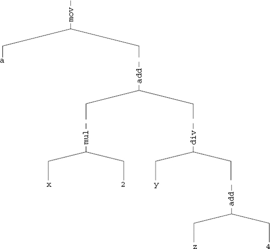
Figure 13.1. An expression tree representing the above C high-level expression. The operators are expressed using their IA-32 instruction names to illustrate how such an expression is translated from a machine code representation to an expression tree.
The idea with this kind of tree is that it is an elegant structured representation of a sequence of arithmetic instructions. Each branch in the tree is roughly equivalent to an instruction in the decompiled program. It is up to the decompiler to perform data-flow analysis on these instructions and construct such a tree. Once a tree is constructed it becomes fairly trivial to produce high-level language expressions by simply scanning the tree. The process of constructing expression trees from individual instructions is discussed below in the data-flow analysis section.
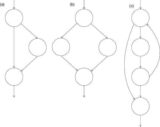
In order to reconstruct high-level control flow information from a low-level representation of a program, decompilers must create a control flow graph (CFG) for each procedure being analyzed. A CFG is a graph representation of the internal flow with a single procedure. The idea with control flow graphs is that they can easily be converted to high-level language control flow constructs such as loops and the various types of branches. Figure 13.2 shows three typical control flow graph structures for an if statement, an if-else statement, and a while loop.
Decompiler front ends perform the opposite function of compiler back ends. Compiler back ends take a compiler's intermediate representation and convert it to the target machine's native assembly language, whereas decompiler front ends take the same native assembly language and convert it back into the decompiler's intermediate representation. The first step in this process is to go over the source executable byte by byte and analyze each instruction, including its operands. These instructions are then analyzed and converted into the decompiler's intermediate representation. This intermediate representation is then slowly improved during the code analysis stage to prepare it for conversion into a high-level language representation by the back end.
Note
Some decompilers don't actually go through the process of disassembling the source executable but instead require the user to run it through a disassembler (such as IDA Pro). The disassembler produces a textual representation of the source program which can then be read and analyzed by the decompiler. This does not directly affect the results of the decompilation process but merely creates a minor inconvenince for the user.
The following sections discuss the individual stages that take place inside a decompiler's front end.
A decompiler front end starts out by simply scanning the individual instructions and converting them into the decompiler's intermediate representation, but it doesn't end there. Directly translating individual instructions often has little value in itself, because some of these instructions only make sense together, as a sequence. There are many architecture specific sequences that are made to overcome certain limitations of the specific architecture. The front end must properly resolve these types of sequences and correctly translate them into the intermediate representation, while eliminating all of the architecture-specific details.
Let's take a look at an example of such a sequence. In the early days of the IA-32 architecture, the floating-point unit was not an integral part of the processor, and was actually implemented on a separate chip (typically referred to as the math coprocessor) that had its own socket on the motherboard. This meant that the two instruction sets were highly isolated from one another, which imposed some limitations. For example, to compare two floating-point values, one couldn't just compare and conditionally branch using the standard conditional branch instructions. The problem was that the math coprocessor couldn't directly update the EFLAGS register (nowadays this is easy, because the two units are implemented on a single chip). This meant that the result of a floating-point comparison was written into a separate floating-point status register, which then had to be loaded into one of the general-purpose registers, and from there it was possible to test its value and perform a conditional branch. Let's look at an example.
00401000    FLD DWORD PTR [ESP+4]
00401004    FCOMP DWORD PTR [ESP+8]
00401008    FSTSW AX
0040100A    TEST AH,41
0040100D    JNZ SHORT 0040101D
This snippet loads one floating-point value into the floating-point stack (essentially like a floating-point register), and compares another value against the first value. Because the older FCOMP instruction is used, the result is stored in the floating-point status word. If the code were to use the newer FCOMIP instruction, the outcome would be written directly into EFLAGS, but this is a newer instruction that didn't exist in older versions of the processor. Because the result is stored in the floating-point status word, you need to somehow get it out of there in order to test the result of the comparison and perform a conditional branch. This is done using the FSTSW instruction, which copies the floating-point status word into the AX register. Once that value is in AX, you can test the specific flags and perform the conditional branch.
The bottom line of all of this is that to translate this sequence into the decompiler's intermediate representation (which is not supposed to contain any architecture-specific details), the front end must "understand" this sequence for what it is, and eliminate the code that tests for specific flags (the constant 0x41) and so on. This is usually implemented by adding specific code in the front end that knows how to decipher these types of sequences.
The code generated by a decompiler's front end is represented in a graph structure, where each code block is called a basic block (BB). This graph structure simply represents the control flow instructions present in the low-level machine code. Each BB ends with a control flow instruction such as a branch instruction, a call, or a ret, or with a label that is referenced by some branch instruction elsewhere in the code (because labels represent a control flow join).
Blocks are defined for each code segment that is referenced elsewhere in the code, typically by a branch instruction. Additionally, a BB is created after every conditional branch instruction, so that a conditional branch instruction can either flow into the BB representing the branch target address or into the BB that contains the code immediately following the condition. This concept is illustrated in Figure 13.3. Note that to improve readability the actual code in Figure 13.3 is shown as IA-32 assembly language code, whereas in most decompilers BBs are represented using the decompiler's internal instruction set.
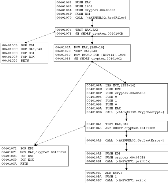
Figure 13.3. An unstructured control flow graph representing branches in the original program. The dotted arrows represent conditional branch instructions while the plain ones represent fall-through cases—this is where execution proceeds when a branch isn't taken.
The control flow graph Figure 13.3 is quite primitive. It is essentially a graphical representation of the low-level control flow statement in the program. It is important to perform this simple analysis at this early stage in decompilation to correctly break the program into basic blocks. The process of actually structuring these graphs into a representation closer to the one used by high-level languages is performed later, during the control flow analysis stage.
Strictly speaking, a decompiler doesn't have an optimizing stage. After all, you're looking to produce a high-level language representation from a binary executable, and not to "improve" the program in any way. On the contrary, you want the output to match the original program as closely as possible. In reality, this optimizing, or code-improving, phase in a decompiler is where the program is transformed from a low-level intermediate representation to a higher-level intermediate representation that is ready to be transformed into a high-level language code. This process could actually be described as the opposite of the compiler's optimization process—you're trying to undo many of the compiler's optimizations.
The code analysis stage is where much of the interesting stuff happens. Decompilation literature is quite scarce, and there doesn't seem to be an official term for this stage, so I'll just name it the code analysis stage, even though some decompiler researchers simply call it the middle-end.
The code analysis stage starts with an intermediate representation of the program that is fairly close to the original assembly language code. The program is represented using an instruction set similar to the one discussed in the previous section, but it still lacks any real expressions. The code analysis process includes data-flow analysis, which is where these expressions are formed, type analysis which is where complex and primitive data types are detected, and control flow analysis, which is where high-level control flow constructs are recovered from the unstructured control flow graph created by the front end. These stages are discussed in detail in the following sections.
Data-flow analysis is a critical stage in the decompilation process. This is where the decompiler analyzes the individual, seemingly unrelated machine instructions and makes the necessary connections between them. The connections are created by tracking the flow of data within those instructions and analyzing the impact each individual instruction has on registers and memory locations. The resulting information from this type of analysis can be used for a number of different things in the decompilation process. It is required for eliminating the concept of registers and operations performed on individual registers, and also for introducing the concept of variables and long expressions that are made up of several machine-level instructions. Data-flow analysis is also where conditional codes are eliminated. Conditional codes are easily decompiled when dealing with simple comparisons, but they can also be used in other, less obvious ways.
Let's look at a trivial example where you must use data-flow analysis in order for the decompiler to truly "understand" what the code is doing. Think of function return values. It is customary for IA-32 code to use the EAX register for passing return values from a procedure to its caller, but a decompiler cannot necessarily count on that. Different compilers might use different conventions, especially when functions are defined as static and the compiler controls all points of entry into the specific function. In such a case, the compiler might decide to use some other register for passing the return value. How does a decompiler know which register is used for passing back return values and which registers are used for passing parameters into a procedure? This is exactly the type of problem addressed by data-flow analysis.
Data-flow analysis is performed by defining a special notation that simplifies this process. This notation must conveniently represent the concept of defining a register, which means that it is loaded with a new value and using a register, which simply means its value is read. Ideally, such a representation should also simplify the process of identifying various points in the code where a register is defined in parallel in two different branches in the control flow graph.
The next section describes SSA, which is a commonly used notation for implementing data-flow analysis (in both compilers and decompilers). After introducing SSA, I proceed to demonstrate areas in the decompilation process where data-flow analysis is required.
Single static assignment (SSA) is a special notation commonly used in compilers that simplifies many data-flow analysis problems in compilers and can assist in certain optimizations and register allocation. The idea is to treat each individual assignment operation as a different instance of a single variable, so that x becomes x0, x1, x2, and so on with each new assignment operation. SSA can be useful in decompilation because decompilers have to deal with the way compilers reuse registers within a single procedure. It is very common for procedures that use a large number of variables to use a single register for two or more different variables, often containing a different data type.
One prominent feature of SSA is its support of

mov esi1, 0         ; Define esi1
   cmp eax1, esi1
   jne NotEquals
   mov esi2, 7         ; Define esi2
   jmp  After
NotEquals:
   mov  esi3, 3         ; Define esi3
After:
   esi4 = ø(esi2, esi3)  ; Define esi4
   mov eax2, esi4        ; Define eax2
In this example, it can be clearly seen how each new assignment into ESI essentially declares a new logical register. The definitions of ESI2 and ESI3 take place in two separate branches on the control flow graph, meaning that only one of these assignments can actually take place while the code is running. This is specified in the definition of ESI4, which is defined using a
Most processor architectures are based on register transfer languages (RTL), which means that they must load values into registers in order to use them. This means that the average program includes quite a few register load and store operations where the registers are merely used as temporary storage to enable certain instructions access to data. Part of the data-flow analysis process in a decompiler involves the elimination of such instructions to improve the readability of the code.
Let's take the following code sequence as an example:
mov        eax, DWORD PTR _z$[esp+36]
lea        ecx, DWORD PTR [eax+4]
mov        eax, DWORD PTR _y$[esp+32]
cdq
idiv    ecx
mov        edx, DWORD PTR _x$[esp+28]
lea        eax, DWORD PTR [eax+edx*2]
In this code sequence each value is first loaded into a register before it is used, but the values are only used in the context of this sample—the contents of EDX and ECX are discarded after this code sequence (EAX is used for passing the result to the caller).
If you directly decompile the preceding sequence into a sequence of assignment expressions, you come up with the following output:
Variable1 = Param3;
Variable2 = Variable1 + 4;
Variable1 = Param2;
Variable1 = Variable1 / Variable2
Variable3 = Param1;
Variable1 = Variable1 + Variable3 * 2;
Even though this is perfectly legal C code, it is quite different from anything that a real programmer would ever write. In this sample, a local variable was assigned to each register being used, which is totally unnecessary considering that the only reason that the compiler used registers is that many instructions simply can't work directly with memory operands. Thus it makes sense to track the flow of data in this sequence and eliminate all temporary register usage. For example, you would replace the first two lines of the preceding sequence with:
Variable2 = Param3 + 4;
So, instead of first loading the value of Param3 to a local variable before using it, you just use it directly. If you look at the following two lines, the same principle can be applied just as easily. There is really no need for storing either Param2 nor the result of Param3 + 4, you can just compute that inside the division expression, like this:
Variable1 = Param2 / (Param3 + 4);
The same goes for the last two lines: You simply carry over the expression from above and propagate it. This gives you the following complex expression:
Variable1 = Param2 / (Param3 + 4) + Param1 * 2;
The preceding code is obviously far more human-readable. The elimination of temporary storage registers is obviously a critical step in the decompilation process. Of course, this process should not be overdone. In many cases, registers represent actual local variables that were defined in the original program. Eliminating them might reduce program readability.
In terms of implementation, one representation that greatly simplifies this process is the SSA notation described earlier. That's because SSA provides a clear picture of the lifespan of each register value and simplifies the process of identifying ambiguous cases where different control flow paths lead to different assignment instructions on the same register. This enables the decompiler to determine when propagation should take place and when it shouldn't.
After you eliminate all temporary registers during the register copy propagation process, you're left with registers that are actually used as variables. These are easy to identify because they are used during longer code sequences compared to temporary storage registers, which are often loaded from some memory address, immediately used in an instruction, and discarded. A register variable is typically defined at some point in a procedure and is then used (either read or updated) more than once in the code.
Still, the simple fact is that in some cases it is impossible to determine whether a register originated in a variable in the program source code or whether it was just allocated by the compiler for intermediate storage. Here is a trivial example of how that happens:
int MyVariable = x * 4;
SomeFunc1(MyVariable);
SomeFunc2(MyVariable);
SomeFunc3(MyVariable);
MyVariable++;
SomeFunc4(MyVariable);
In this example the compiler is likely to assign a register for MyVariable, calculate x * 4 into it, and push it as the parameter in the first three function calls. At that point, the register would be incremented and pushed as a parameter for the last function call. The problem is that this is exactly the same code most optimizers would produce for the example that follows as well:
SomeFunc1(x * 4);
SomeFunc2(x * 4);
SomeFunc3(x * 4);
SomeFunc4(x * 4 + 1);
In this case, the compiler is smart enough to realize that x * 4 doesn't need to be calculated four times. Instead it just computes x * 4 into a register and pushes that value into each function call. Before the last call to SomeFunc4 that register is incremented and is then passed into SomeFunc4, just as in the previous example where the variable was explicitly defined. This is good example of how information is irretrievably lost during the compilation process. A decompiler would have to employ some kind of heuristic to decide whether to declare a variable for x * 4 or simply duplicate that expression wherever it is used.
It should be noted that this is more of a style and readability issue that doesn't really affect the meaning of the code. Still, in very large functions that use highly complex expressions, it might make a significant impact on the overall readability of the generated code.
Another thing data-flow analysis is good for is data type propagation. Decompilers receive type information from a variety of sources and type-analysis techniques. Propagating that information throughout the program as much as possible can do wonders to improve the readability of decompiled output. Let's take a powerful technique for extracting type information and demonstrate how it can benefit from type propagation.
It is a well-known practice to gather data type information from library calls and system calls [Guilfanov]. The idea is that if you can properly identify calls to known functions such as system calls or runtime library calls, you can easily propagate data types throughout the program and greatly improve its readability. First let's consider the simple case of external calls made to known system functions such as KERNEL32!CreateFileA. Upon encountering such a call, a decompiler can greatly benefit from the type information known about the call. For example, for this particular API it is known that its return value is a file handle and that the first parameter it receives is a pointer to an ASCII file name.
This information can be propagated within the current procedure to improve its readability because you now know that the register or storage location from which the first parameter is taken contains a pointer to a file name string. Depending on where this value comes from, you can enhance the program's type information. If for instance the value comes from a parameter passed to the current procedure, you now know the type of this parameter, and so on.
In a similar way, the value returned from this function can be tracked and correctly typed throughout this procedure and beyond. If the return value is used by the caller of the current procedure, you now know that the procedure also returns a file handle type.
This process is most effective when it is performed globally, on the entire program. That's because the decompiler can recursively propagate type information throughout the program and thus significantly improve overall output quality. Consider the call to CreateFileA from above. If you propagate all type information deduced from this call to both callers and callees of the current procedure, you wind up with quite a bit of additional type information throughout the program.
Depending on the specific platform for which the executable was created, accurate type information is often not available in binary executables, certainly not directly. Higher-level bytecodes such as the Java bytecode and MSIL do contain accurate type information for function arguments, and class members (MSIL also has local variable data types, which are not available in the Java bytecode), which greatly simplifies the decompilation process. Native IA-32 executables (and this is true for most other processor architectures as well) contain no explicit type information whatsoever, but type information can be extracted using techniques such as the constraint-based techniques described in [Mycroft]. The following sections describe techniques for gathering simple and complex data type information from executables.
When a register is defined (that is, when a value is first loaded into it) there is often no data type information available whatsoever. How can the decompiler determine whether a certain variable contains a signed or unsigned value, and how long it is (char, short int, and so on)? Because many instructions completely ignore primitive data types and operate in the exact same way regardless of whether a register contains a signed or an unsigned value, the decompiler must scan the code for instructions that are type sensitive. There are several examples of such instructions.
For detecting signed versus unsigned values, the best method is to examine conditional branches that are based on the value in question. That's because there are different groups of conditional branch instructions for signed and unsigned operands (for more information on this topic please see Appendix A). For example, the JG instruction is used when comparing signed values, while the JA instruction is used when comparing unsigned values. By locating one of these instructions and associating it with a specific register, the decompiler can propagate information on whether this register (and the origin of its current value) contains a signed or an unsigned value.
The MOVZX and MOVSX instructions make another source of information regarding signed versus unsigned values. These instructions are used when up-converting a value from 8 or 16 bits to 32 bits or from 8 bits to 16 bits. Here, the compiler must select the right instruction to reflect the exact data type being up-converted. Signed values must be sign extended using the MOVSX instruction, while unsigned values must be zero extended, using the MOVZX instruction. These instructions also reveal the exact length of a variable (before the up-conversion and after it). In cases where a shorter value is used without being up-converted first, the exact size of a specific value is usually easy to determine by observing which part of the register is being used (the full 32 bits, the lower 16 bits, and so on).
Once information regarding primitive data types is gathered, it makes a lot of sense to propagate it globally, as discussed earlier. This is generally true in native code decompilation—you want to take every tiny piece of relevant information you have and capitalize on it as much as possible.
How do decompilers deal with more complex data constructs such as structs and arrays? The first step is usually to establish that a certain register holds a memory address. This is trivial once an instruction that uses the register's value as a memory address is spotted somewhere throughout the code. At that point decompilers rely on the type of pointer arithmetic performed on the address to determine whether it is a struct or array and to create a definition for that data type.
Code sequences that add hard-coded constants to pointers and then access the resulting memory address can typically be assumed to be accessing structs. The process of determining the specific primitive data type of each member can be performed using the primitive data type identification techniques from above.
Arrays are typically accessed in a slightly different way, without using hard-coded offsets. Because array items are almost always accessed from inside a loop, the most common access sequence for an array is to use an index and a size multiplier. This makes arrays fairly easy to locate. Memory addresses that are calculated by adding a value multiplied by a constant to the base memory address are almost always arrays. Again the data type represented by the array can hopefully be determined using our standard type-analysis toolkit.
Note
Sometimes a struct or array can be accessed without loading a dedicated register with the address to the data structure. This typically happens when a specific array item or struct member is specified and when that data structure resides on the stack. In such cases, the compiler can use hard-coded stack offsets to access individual fields in the struct or items in the array. In such cases, it becomes impossible to distinguish complex data types from simple local variables that reside on the stack.
In some cases, it is just not possible to recover array versus data structure information. This is most typical with arrays that are accessed using hard-coded indexes. The problem is that in such cases compilers typically resort to a hard-coded offset relative to the starting address of the array, which makes the sequence look identical to a struct access sequence.
Take the following code snippet as an example:
mov eax, DWORD PTR [esp-4]
mov DWORD PTR [eax], 0
mov DWORD PTR [eax+4], 1
mov DWORD PTR [eax+8], 2
The problem with this sequence is that you have no idea whether EAX represents a pointer to a data structure or an array. Typically, array items are not accessed using hard-coded indexes, and structure members are, but there are exceptions. In most cases, the preceding machine code would be produced by accessing structure members in the following fashion:
void foo1(TESTSTRUCT *pStruct)
{
  pStruct->a = FALSE;
  pStruct->b = TRUE;
  pStruct->c = SOMEFLAG; // SOMEFLAG == 2
}
The problem is that without making too much of an effort I can come up with at least one other source code sequence that would produce the very same assembly language code. The obvious case is if EAX represents an array and you access its first three 32-bit items and assign values to them, but that's a fairly unusual sequence. As I mentioned earlier, arrays are usually accessed via loops. This brings us to aggressive loop unrolling performed by some compilers under certain circumstances. In such cases, the compiler might produce the above assembly language sequence (or one very similar to it) even if the source code contained a loop. The following source code is an example—when compiled using the Microsoft C/C++ compiler with the Maximize Speed settings, it produces the assembly language sequence you saw earlier:
void foo2(int *pArray)
{
  for (int i = 0; i < 3; i++)
    pArray[i] = i;
}
This is another unfortunate (yet somewhat extreme) example of how information is lost during the compilation process. From a decompiler's standpoint, there is no way of knowing whether EAX represents an array or a data structure. Still, because arrays are rarely accessed using hard-coded offsets, simply assuming that a pointer calculated using such offsets represents a data structure would probably work for 99 percent of the code out there.
Control flow analysis is the process of converting the unstructured control flow graphs constructed by the front end into structured graphs that represent high-level language constructs. This is where the decompiler converts abstract blocks and conditional jumps to specific control flow constructs that represent high-level concepts such as pretested and posttested loops, two-way conditionals, and so on.
A thorough discussion of these control flow constructs and the way they are implemented by most modern compilers is given in Appendix A. The actual algorithms used to convert unstructured graphs into structured control flow graphs are beyond the scope of this book. An extensive coverage of these algorithms can be found in [Cifuentes2], [Cifuentes3].
Much of the control flow analysis is straightforward, but there are certain compiler idioms that might warrant special attention at this stage in the process. For example, many compilers tend to convert pretested loops to posttested loops, while adding a special test before the beginning of the loop to make sure that it is never entered if its condition is not satisfied. This is done as an optimization, but it can somewhat reduce code readability from the decompilation standpoint if it is not properly handled. The decompiler would perform a literal translation of this layout and would present the initial test as an additional if statement (that obviously never existed in the original program source code), followed by a do...while loop. It might make sense for a decompiler writer to identify this case and correctly structure the control flow graph to represent a regular pretested loop. Needless to say, there are likely other cases like this where compiler optimizations alter the control flow structure of the program in ways that would reduce the readability of decompiled output.
Most executables contain significant amounts of library code that is linked into the executable. During the decompilation process it makes a lot of sense to identify these functions, mark them, and avoid decompiling them. There are several reasons why this is helpful:
Decompiling all of this library code is often unnecessary and adds redundant code to the decompiler's output. By identifying library calls you can completely eliminate library code and increase the quality and relevance of our decompiled output.
Properly identifying library calls means additional "symbols" in the program because you now have the names of every internal library call, which greatly improves the readability of the decompiled output.
Once you have properly identified library calls you can benefit from the fact that you have accurate type information for these calls. This information can be propagated across the program (see the section on data type propagation earlier in this chapter) and greatly improve readability.
Techniques for accurately identifying library calls were described in [Emmerik1]. Without getting into too much detail, the basic idea is to create signatures for library files. These signatures are simply byte sequences that represent the first few bytes of each function in the library. During decompilation the executable is scanned for these signatures (using a hash to make the process efficient), and the addresses of all library functions are recorded. The decompiler generally avoids decompilation of such functions and simply incorporates the details regarding their data types into the type-analysis process.
A decompiler's back end is responsible for producing actual high-level language code from the processed code that is produced during the code analysis stage. The back end is language-specific, and just as a compiler's back end is interchangeable to allow the compiler to support more than one processor architecture, so is a decompiler's back end. It can be fairly easily replaced to get the decompiler to produce different high-level language outputs.
Let's run a brief overview of how the back end produces code from the instructions in the intermediate representation. Instructions such as the assignment instruction typically referred to as asgn are fairly trivial to process because asgn already contains expression trees that simply need to be rendered as text. The call and ret instructions are also fairly trivial. During data-flow analysis the decompiler prepares an argument list for call instructions and locates the return value for the ret instruction. These are stored along with the instructions and must simply be printed in the correct syntax (depending on the target language) during the code-generation phase.
Probably the most complex step in this process is the creation of control flow statements from the structured control flow graph. Here, the decompiler must correctly choose the most suitable high-level language constructs for representing the control flow graph. For instance, most high-level languages support a variety of loop constructs such as "do...while", "while...", and "for..." loops. Additionally, depending on the specific language, the code might have unconditional jumps inside the loop body. These must be translated to keywords such as break or continue, assuming that such keywords (or ones equivalent to them) are supported in the target language.
Generating code for two-way or n-way conditionals is fairly straightforward at this point, considering that the conditions have been analyzed during the code-analysis stage. All that's needed here is to determine the suitable language construct and produce the code using the expression tree found in the conditional statement (typically referred to as jcond). Again, unstructured elements in the control flow graph that make it past the analysis stage are typically represented using goto statements (think of an unconditional jump into the middle of a conditional block or a loop).
At this point you might be thinking that you haven't really seen (or been able to find) that many working IA-32 decompilers, so where are they? Well, the fact is that at the time of writing there really aren't that many fully functional IA-32 decompilers, and it really looks as if this technology has a way to go before it becomes fully usable.
The two native IA-32 decompilers currently in development to the best of my knowledge are Andromeda and Boomerang. Both are already partially usable and one (Boomerang) has actually been used in the recovery of real production source code in a commercial environment [Emmerik2]. This report describes a process in which relatively large amounts of code were recovered while gradually improving the decompiler and fixing bugs to improve its output. Still, most of the results were hand-edited to improve their readability, and this project had a good starting point: The original source code of an older, prototype version of the same product was available.
This concludes the relatively brief survey of the fascinating field of decompilation. In this chapter, you have learned a bit about the process and algorithms involved in decompilation. You have also seen some demonstrations of the type of information available in binary executables, which gave you an idea on what type of output you could expect to see from a cutting-edge decompiler.
It should be emphasized that there is plenty more to decompilation. I have intentionally avoided discussing the details of decompilation algorithms to avoid turning this chapter into a boring classroom text. If you're interested in learning more, there are no books that specifically discuss decompilation at the time of writing, but probably the closest thing to a book on this topic is a PhD thesis written by Christina Cifuentes, Reverse Compilation Techniques [Cifuentes2]. This text provides a highly readable introduction to the topic and describes in detail the various algorithms used in decompilation. Beyond this text most of the accumulated knowledge can be found in a variety of research papers on this topic, most of which are freely available online.
As for the question of what to expect from binary decompilation, I'd summarize by saying binary decompilation is possible—it all boils down to setting people's expectations. Native code decompilation is "no silver bullet", to borrow from that famous line by Brooks—it cannot bring back 100 percent accurate high-level language code from executable binaries. Still, a working native code decompiler could produce an approximation of the original source code and do wonders to the reversing process by dramatically decreasing the amount of time it takes to reach an understanding of a complex program for which source code is not available.
There is certainly a lot to hope for in the field of binary decompilation. We have not yet seen what a best-of-breed native code decompiler could do when it is used with high quality library signatures and full-blown prototypes for operating system calls, and so on. I always get the impression that many people don't fully realize just how good an output could be expected from such a tool. Hopefully, time will tell.