Table of Contents for
Reversing: Secrets of Reverse Engineering
 Reversing: Secrets of Reverse Engineering
Published by
John Wiley & Sons, 2005
Reversing: Secrets of Reverse Engineering
Published by
John Wiley & Sons, 2005
- Copyright
- Credits
- Foreword
- Acknowledgments
- Introduction
- I. Reversing 101
- 1. Foundations
- 2. Low-Level Software
- 3. Windows Fundamentals
- 4. Reversing Tools
- II. Applied Reversing
- 5. Beyond the Documentation
- 6. Deciphering File Formats
- 7. Auditing Program Binaries
- 8. Reversing Malware
- III. Cracking
- 9. Piracy and Copy Protection
- 10. Antireversing Techniques
- 11. Breaking Protections
- IV. Beyond Disassembly
- 12. Reversing .NET
- 13. Decompilation
- A. Deciphering Code Structures
- B. Understanding Compiled Arithmetic
- C. Deciphering Program Data
- D. Citations
It would be safe to say that any properly designed program is designed around data. What kind of data must the program manage? What would be the most accurate and efficient representation of that data within the program? These are really the most basic questions that any skilled software designer or developer must ask.
The same goes for reversing. To truly understand a program, reversers must understand its data. Once the general layout and purpose of the program's key data structures are understood, specific code area of interest will be relatively easy to decipher.
This appendix covers a variety of topics related to low-level data management in a program. I start out by describing the stack and how it is used by programs and proceed to a discussion of the most basic data constructs used in programs, such as variables, and so on. The next section deals with how data is laid out in memory and describes (from a low-level perspective) common data constructs such as arrays and other types of lists. Finally, I demonstrate how classes are implemented in low-level and how they can be identified while reversing.
The stack is basically a continuous chunk of memory that is organized into virtual "layers" by each procedure running in the system. Memory within the stack is used for the lifetime duration of a function and is freed (and can be reused) once that function returns.
The following sections demonstrate how stacks are arranged and describe the various calling conventions which govern the basic layout of the stack.
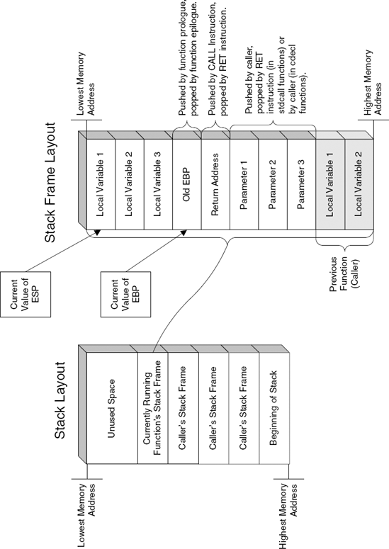
A stack frame is the area in the stack allocated for use by the currently running function. This is where the parameters passed to the function are stored, along with the return address (to which the function must jump once it completes), and the internal storage used by the function (these are the local variables the function stores on the stack).
The specific layout used within the stack frame is critical to a function because it affects how the function accesses the parameters passed to it and it function stores its internal data (such as local variables). Most functions start with a prologue that sets up a stack frame for the function to work with. The idea is to allow quick-and-easy access to both the parameter area and the local variable area by keeping a pointer that resides between the two. This pointer is usually stored in an auxiliary register (usually EBP), while ESP (which is the primary stack pointer) remains available for maintaining the current stack position. The current stack position is important in case the function needs to call another function. In such a case the region below the current position of ESP will be used for creating a new stack frame that will be used by the callee.
Figure C.1 demonstrates the general layout of the stack and how a stack frame is laid out.
The ENTER and LEAVE instructions are built-in tools provided by the CPU for implementing a certain type of stack frame. They were designed as an easy-to-use, one-stop solution to setting up a stack frame in a procedure.
ENTER sets up a stack frame by pushing EBP into the stack and setting it to point to the top of the local variable area (see Figure C.1). ENTER also supports the management of nested stack frames, usually within the same procedure (in languages that support such nested blocks). For nesting to work, the code issuing the ENTER code must specify the current nesting level (which makes this feature less relevant for implementing actual procedure calls). When a nesting level is provided, the instruction stores the pointer to the beginning of every currently active stack frame in the procedure's stack frame. The code can then use those pointers for accessing the other currently active stack frames.
ENTER is a highly complex instruction that performs the work of quite a few instructions. Internally, it is implemented using a fairly lengthy piece of microcode, which creates some performance problems. For this reason most compilers seem to avoid using ENTER, even if they support nested code blocks for languages such as C and C++. Such compilers simply ignore the existence of code blocks while arranging the procedure's local stack layout and place all local variables in a single region.
The LEAVE instruction is ENTER's counterpart. LEAVE simply restores ESP and EBP to their previously stored values. Because LEAVE is a much simpler instruction, many compilers seem to use it in their function epilogue (even though ENTER is not used in the prologue).
A calling convention defines how functions are called in a program. Calling conventions are relevant to this discussion because they govern the way data (such as parameters) is arranged on the stack when a function call is made. It is important that you develop an understanding of calling conventions because you will be constantly running into function calls while reversing, and because properly identifying the calling conventions used will be very helpful in gaining an understanding of the program youtrying to decipher.
Before discussing the individual calling conventions, I should discuss the basic function call instructions, CALL and RET. The CALL instruction pushes the current instruction pointer (it actually stores the pointer to the instruction that follows the CALL) onto the stack and performs an unconditional jump into the new code address.
The RET instruction is CALL's counterpart, and is the last instruction in pretty much every function. RET pops the return address (stored earlier by CALL) into the EIP register and proceeds execution from that address.
The following sections go over the most common calling conventions and describe how they are implemented in assembly language.
The cdecl calling convention is the standard C and C++ calling convention. The unique feature it has is that it allows functions to receive a dynamic number of parameters. This is possible because the caller is responsible for restoring the stack pointer after making a function call, and of course the caller always knows how many parameters it passed. Identifying cdecl calls is fairly simple: Any function that takes one or more parameters through the stack and ends with a simple RET with no operands is most likely a cdecl function.
As the name implies, fastcall is a slightly higher-performance calling convention that uses registers for passing the first two parameters passed to a function. The rest of the parameters are passed through the stack. fastcall was originally a Microsoft specific calling convention but is now supported by most major compilers, so you can expect to see it quite frequently in modern programs. fastcall always uses ECX and EDX to store the first and second function parameters, respectively.
The stdcall calling convention is very common in Windows—it is used by nearly every Windows API and system function. The difference between stdcall and cdecl is that stdcall functions are responsible for clearing their own stack, whereas in cdecl that's the caller's responsibility. stdcall functions typically use the RET instruction for clearing the stack. The RET instruction can optionally receive an operand that specifies the number of bytes to clear from the stack after jumping back to the caller. This means that in stdcall functions the operand passed to RET often exposes the number of bytes passed as parameters, meaning that if you divide that number by 4 you get the number of parameters that the function receives. This can be a very helpful hint for both identifying stdcall functions while reversing and for determining how many parameters such functions take.
This calling convention is used by the Microsoft and Intel compilers when a C++ method function with a static number of parameters is called. A quick technique for identifying such calls is to remember that any function call sequence that loads a valid pointer into ECX and pushes parameters onto the stack, but without using EDX, is a C++ method function call. The idea is that because every C++ method must receive a class pointer (called the this pointer) and is likely to use that pointer extensively, the compiler uses a more efficient technique for passing and storing this particular parameter.
Note
For member functions with a dynamic number of parameters, compilers tend to use cdecl and simply pass the this pointer as the first parameter on the stack.
The following sections deal with the most basic data constructs from a high-level perspective and describe how they are implemented by compilers in the low-level realm. These are the most basic elements in programming such as global variables, local variables, constants, and so on. The benefit of learning how these constructs are implemented is that this knowledge can really simplify the process of identifying such constructs while reversing.
In most programs the data hierarchy starts with one or more global variables. These variables are used as a sort of data root when program data structures are accessed. Often uncovering and mapping these variables is required for developing an understanding of a program. In fact, I often consider searching and mapping global variables to be the first logical step when reversing a program.
In most environments, global variables are quite easy to locate. Global variables typically reside in fixed addresses inside the executable module's data section, and when they are accessed, a hard-coded address must be used, which really makes it easy to spot code that accesses such variables. Here is a quick example:
mov eax, [00403038]
This is a typical instruction that reads a value from a global variable. You pretty much know for a fact that this is a global variable because of that hard-coded address, 0x00403038. Such hard-coded addresses are rarely used by compilers for anything other than global variables. Still, there are several other cases in which compilers use hard-coded addresses, which are discussed in the sidebar titled "Static Variables" and in several other places throughout this appendix.
Local variables are used by programmers for storing any kind of immediate values required by the current function. This includes counters, pointers, and other short-term information. Compilers have two primary options for managing local variables: They can be placed on the stack or they can be stored in a register. These two options are discussed in the next sections.
In many cases, compilers simply preallocate room in the function's stack area for the variable. This is the area on the stack that's right below (or before) the return address and stored base pointer. In most stack frames, EBP points to the end of that region, so that any code requiring access to a local variable must use EBP and subtract a certain offset from it, like this:
mov eax, [ebp - 0x4]
This code reads from EBP – 4, which is usually the beginning of the local variable region. The specific data type of the variable is not known from this instruction, but it is obvious that the compiler is treating this as a full 32-bit value from the fact that EAX is used, and not one of the smaller register sizes. Note that because this variable is accessed using what is essentially a hard-coded offset from EBP, this variable and others around it must have a fixed, predetermined size.
Mapping and naming the local variables in a function is a critical step in the reversing process. Afterward, the process of deciphering the function's logic and flow becomes remarkably simpler!
When developers need to pass parameters that can be modified by the called function and read back by the caller, they just pass their parameters by reference instead of by value. The idea is that instead of actually pushing the value of parameters onto the stack, the caller pushes an address that points to that value. This way, when the called function receives the parameter, it can read the value (by accessing the passed memory address) and write back to it by simply writing to the specified memory address.
This fact makes it slightly easier for reversers to figure out what's going on. When a function is writing into the parameter area of the stack, you know that it is probably just using that space to hold some extra variables, because functions rarely (if ever) return values to their caller by writing back to the parameter area of the stack.
Performance-wise, compilers always strive to store all local variables in registers. Registers are always the most efficient way to store immediate values, and using them always generates the fastest and smallest code (smallest because most instructions have short preassigned codes for accessing registers). Compilers usually have a separate register allocator component responsible for optimizing the generated code's usage of registers. Compiler designers often make a significant effort to optimize these components so that registers are allocated as efficiently as possible because that can have a substantial impact on overall program size and efficiency.
There are several factors that affect the compiler's ability to place a local variable in a register. The most important one is space. There are eight general-purpose registers in IA-32 processors, two of which are used for managing the stack. The remaining six are usually divided between the local variables as efficiently as possible. One important point for reversers to remember is that most variables aren't used for the entire lifetime of the function and can be reused. This can be confusing because when a variable is overwritten, it might be difficult to tell whether the register still represents the same thing (meaning that this is the same old variable) or if it now represents a brand-new variable. Finally, another factor that forces compilers to use memory addresses for local variables is when a variable's address is taken using the & operator—in such cases the compiler has no choice but to place the local variable on the stack.
Imported variables are global variables that are stored and maintained in another binary module (meaning another dynamic module, or DLL). Any binary module can declare global variables as "exported" (this is done differently in different development platforms) and allow other binaries loaded into the same address space access to those variables.
Imported variables are important for reversers for several reasons, the most important being that (unlike other variables) they are usually named. This is because in order to export a variable, the exporting module and the importing module must both reference the same variable name. This greatly improves readability for reversers because they can get at least some idea of what the variable contains through its name. It should be noted that in some cases imported variables might not be named. This could be either because they are exported by ordinals (see Chapter 3) or because their names were intentionally mangled during the build process in order to slow down and annoy reversers.
Identifying imported variables is usually fairly simple because accessing them always involves an additional level of indirection (which, incidentally, also means that using them incurs a slight performance penalty).
A low-level code sequence that accesses an imported variable would usually look something like this:
mov
eax, DWORD PTR [IATAddress]
mov
ebx, DWORD PTR [eax]
In itself, this snippet is quite common—it is code that indirectly reads data from a pointer that points to another pointer. The giveaway is the value of IATAddress. Because this pointer points to the module's Import Address Table, it is relatively easy to detect these types of sequences.
The bottom line is that any double-pointer indirection where the first pointer is an immediate pointing to the current module's Import Address Table should be interpreted as a reference to an imported variable.
C and C++ provide two primary methods for using constants within the code. One is interpreted by the compiler's preprocessor, and the other is interpreted by the compiler's front end along with the rest of the code.
Any constant defined using the #define directive is replaced with its value in the preprocessing stage. This means that specifying the constant's name in the code is equivalent to typing its value. This almost always boils down to an immediate embedded within the code.
The other alternative when defining a constant in C/C++ is to define a global variable and add the const keyword to the definition. This produces code that accesses the constant just as if it were a regular global variable. In such cases, it may or may not be possible to confirm that you're dealing with a constant. Some development tools will simply place the constant in the data section along with the rest of the global variables. The enforcement of the const keyword will be done at compile time by the compiler. In such cases, it is impossible to tell whether a variable is a constant or just a global variable that is never modified.
Other development tools might arrange global variables into two different sections, one that's both readable and writable, and another that is read-only. In such a case, all constants will be placed in the read-only section and you will get a nice hint that you're dealing with a constant.
Thread-local storage is useful for programs that are heavily thread-dependent and than maintain per-thread data structures. Using TLS instead of using regular global variables provides a highly efficient method for managing thread-specific data structures. In Windows there are two primary techniques for implementing thread-local storage in a program. One is to allocate TLS storage using the TLS API. The TLS API includes several functions such as TlsAlloc, TlsGetValue, and TlsSetValue that provide programs with the ability to manage a small pool of thread-local 32-bit values.
Another approach for implementing thread-local storage in Windows programs is based on a different approach that doesn't involve any API calls. The idea is to define a global variable with the declspec(thread) attribute that places the variable in a special thread-local section of the image executable. In such cases the variable can easily be identified while reversing as thread local because it will point to a different image section than the rest of the global variables in the executable. If required, it is quite easy to check the attributes of the section containing the variable (using a PE-dumping tool such as DUMPBIN) and check whether it's thread-local storage. Note that the thread attribute is generally a Microsoft-specific compiler extension.
A data structure is any kind of data construct that is specifically laid out in memory to meet certain program needs. Identifying data structures in memory is not always easy because the philosophy and idea behind their organization are not always known. The following sections discuss the most common layouts and how they are implemented in assembly language. These include generic data structures, arrays, linked lists, and trees.
A generic data structure is any chunk of memory that represents a collection of fields of different data types, where each field resides at a constant distance from the beginning of the block. This is a very broad definition that includes anything defined using the struct keyword in C and C++ or using the class keyword in C++. The important thing to remember about such structures is that they have a static arrangement that is defined at compile time, and they usually have a static size. It is possible to create a data structure where the last member is a variable-sized array and that generates code that dynamically allocates the structure in runtime based on its calculated size. Such structures rarely reside on the stack because normally the stack only contains fixed-size elements.
Data structures are usually aligned to the processor's native word-size boundaries. That's because on most systems unaligned memory accesses incur a major performance penalty. The important thing to realize is that even though data structure member sizes might be smaller than the processor's native word size, compilers usually align them to the processor's word size.
A good example would be a Boolean member in a 32-bit-aligned structure. The Boolean uses 1 bit of storage, but most compilers will allocate a full 32-bit word for it. This is because the wasted 31 bits of space are insignificant compared to the performance bottleneck created by getting the rest of the data structure out of alignment. Remember that the smallest unit that 32-bit processors can directly address is usually 1 byte. Creating a 1-bit-long data member means that in order to access this member and every member that comes after it, the processor would not only have to perform unaligned memory accesses, but also quite a bit of shifting and ANDing in order to reach the correct member. This is only worthwhile in cases where significant emphasis is placed on lowering memory consumption.
Even if you assign a full byte to your Boolean, you'd still have to pay a significant performance penalty because members would lose their 32-bit alignment. Because of all of this, with most compilers you can expect to see mostly 32-bit-aligned data structures when reversing.
An array is simply a list of data items stored sequentially in memory. Arrays are the simplest possible layout for storing a list of items in memory, which is probably the reason why arrays accesses are generally easy to detect when reversing. From the low-level perspective, array accesses stand out because the compiler almost always adds some kind of variable (typically a register, often multiplied by some constant value) to the object's base address. The only place where an array can be confused with a conventional data structure is where the source code contains hard-coded indexes into the array. In such cases, it is impossible to tell whether you're looking at an array or a data structure, because the offset could either be an array index or an offset into a data structure.
Note
Unlike generic data structures, compilers don't typically align arrays, and items are usually placed sequentially in memory, without any spacing for alignment. This is done for two primary reasons. First of all, arrays can get quite large, and aligning them would waste huge amounts of memory. Second, array items are often accessed sequentially (unlike structure members, which tend to be accessed without any sensible order), so that the compiler can emit code that reads and writes the items in properly sized chunks regardless of their real size.
Generic data type arrays are usually arrays of pointers, integers, or any other single-word-sized items. These are very simple to manage because the index is simply multiplied by the machine's word size. In 32-bit processors this means multiplying by 4, so that when a program is accessing an array of 32-bit words it must simply multiply the desired index by 4 and add that to the array's starting address in order to reach the desired item's memory address.
Data structure arrays are similar to conventional arrays (that contain basic data types such as integers, and so on), except that the item size can be any value, depending on the size of the data structure. The following is an average data-structure array access code.
mov       eax, DWORD PTR [ebp - 0x20]
shl       eax, 4
mov       ecx, DWORD PTR [ebp - 0x24]
cmp       DWORD PTR [ecx+eax+4], 0
This snippet was taken from the middle of a loop. The ebp – 0x20 local variable seems to be the loop's counter. This is fairly obvious because ebp – 0x20 is loaded into EAX, which is shifted left by 4 (this is the equivalent of multiplying by 16, see Appendix B). Pointers rarely get multiplied in such a way—it is much more common with array indexes. Note that while reversing with a live debugger it is slightly easier to determine the purpose of the two local variables because you can just take a look at their values.
After the multiplication ECX is loaded from ebp – 0x24, which seems to be the array's base pointer. Finally, the pointer is added to the multiplied index plus 4. This is a classic data-structure-in-array sequence. The first variable (ECX) is the base pointer to the array. The second variable (EAX) is the current byte offset into the array. This was created by multiplying the current logical index by the size of each item, so you now know that each item in your array is 16 bytes long. Finally, the program adds 4 because this is how it accesses a specific member within the structure. In this case the second item in the structure is accessed.
Linked lists are a popular and convenient method of arranging a list in memory. Programs frequently use linked lists in cases where items must frequently be added and removed from different parts of the list. A significant disadvantage with linked lists is that items are generally not directly accessible through their index, as is the case with arrays (though it would be fair to say that this only affects certain applications that need this type of direct access). Additionally, linked lists have a certain memory overhead associated with them because of the inclusion of one or two pointers along with every item on the list.
From a reversing standpoint, the most significant difference between an array and a linked list is that linked list items are scattered in memory and each item contains a pointer to the next item and possibly to the previous item (in doubly linked lists). This is different from array items which are stored sequentially in memory. The following sections discuss singly linked lists and doubly linked lists.
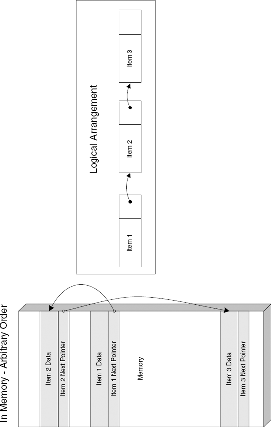
Singly linked lists are simple data structures that contain a combination of the "payload", and a "next" pointer, which points to the next item. The idea is that the position of each item in memory has nothing to do with the logical order of items in the list, so that when item order changes, or when items are added and removed, no memory needs to be copied. Figure C.2 shows how a linked list is arranged logically and in memory.
The following code demonstrates how a linked list is traversed and accessed in a program:
mov         esi, DWORD PTR [ebp + 0x10]
test       esi, esi
je         AfterLoopLoop
Start:
mov        eax, DWORD PTR [esi+88]
mov        ecx, DWORD PTR [esi+84]
push       eax
push       ecx
call       ProcessItem
test       al, al
jne        AfterLoop
mov        esi, DWORD PTR [esi+196]
test       esi, esi
jne        LoopStart
AfterLoop:
.
.
.
This code section is a common linked-list iteration loop. In this example, the compiler has assigned the current item's pointer into ESI—what must have been called pCurrentItem (or something of that nature) in the source code. In the beginning, the program loads the current item variable with a value from ebp + 0x10. This is a parameter that was passed to the current function—it is most likely the list's head pointer.
The loop's body contains code that passes the values of two members from the current item to a function. I've named this function ProcessItem for the sake of readability. Note that the return value from this function is checked and that the loop is interrupted if that value is nonzero.
If you take a look near the end, you will see the code that accesses the current item's "next" member and replaces the current item's pointer with it. Notice that the offset into the next item is 196. That is a fairly high number, indicating that you're dealing with large items, probably a large data structure. After loading the "next" pointer, the code checks that it's not NULL and breaks the loop if it is. This is most likely a while loop that checks the value of pCurrentItem. The following is the original source code for the previous assembly language snippet.
PLIST_ITEM    pCurrentItem = pListHead
while (pCurrentItem)
{
       if (ProcessItem(pCurrentItem->SomeMember,
                                     pCurrentItem->SomeOtherMember))
                                     break;

       pCurrentItem = pCurrentItem->pNext;
}
Notice how the source code uses a while loop, even though the assembly language version clearly used an if statement at the beginning, followed by a do...while() loop. This is a typical loop optimization technique that was mentioned in Appendix A.
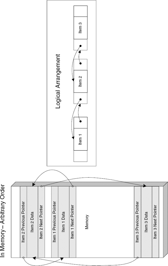
A doubly linked list is the same as a singly linked list with the difference that each item also contains a "previous" pointer that points to the previous item in the list. This makes it very easy to delete an item from the middle of the list, which is not a trivial operation with singly linked lists. Another advantage is that programs can traverse the list backward (toward the beginning of the list) if they need to. Figure C.3 demonstrates how a doubly linked list is arranged logically and in memory.
A binary tree is essentially a compromise between a linked list and an array. Like linked lists, trees provide the ability to quickly add and remove items (which can be a very slow and cumbersome affair with arrays), and they make items very easily accessible (though not as easily as with a regular array).
Binary trees are implemented similarly to linked lists where each item sits separately in its own block of memory. The difference is that with binary trees the links to the other items are based on their value, or index (depending on how the tree is arranged on what it contains).
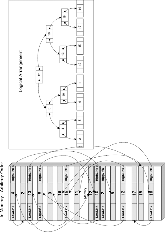
A binary tree item usually contains two pointers (similar to the "prev" and "next" pointers in a doubly linked list). The first is the "left-hand" pointer that points to an item or group of items of lower or equal indexes. The second is the "right-hand" pointer that points items of higher indexes. When searching a binary tree, the program simply traverses the items and jumps from node to node looking for one that matches the index it's looking for. This is a very efficient method for searching through a large number of items. Figure C.4 shows how a tree is laid out in memory and how it's logically arranged.
A class is basically the C++ term (though that term is used by a number of high-level object-oriented languages) for an "object" in the object-oriented design sense of the word. These are logical constructs that contain a combination of data and of code that operates on that data.
Classes are important constructs in object-oriented languages, because pretty much every aspect of the program revolves around them. Therefore, it is important to develop an understanding of how they are implemented and of the various ways to identify them while reversing. In this section I will be demonstrating how the various aspects of the average class are implemented in assembly language, including data members, code members (methods), and virtual members.
A plain-vanilla class with no inheritance is essentially a data structure with associated functions. The functions are automatically configured to receive a pointer to an instance of the class (the this pointer) as their first parameter (this is the this pointer I discussed earlier that's typically passed via ECX). When a program accesses the data members of a class the code generated will be identical to the code generated when accessing a plain data structure. Because data accesses are identical, you must use member function calls in order to distinguish a class from a regular data structure.
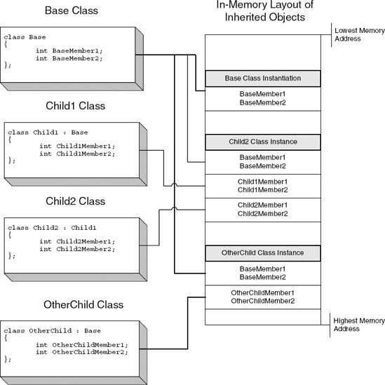
The powerful features of object-oriented programming aren't really apparent until one starts using inheritance. Inheritance allows for the creation of a generic base class that has multiple descendants, each with different functionality. When an object is instantiated, the instantiating code must choose which type of object is being created. When the compiler encounters such an instantiation, it determines the exact data type being instantiated, and generates code that allocates the object plus all of its ancestors. The compiler arranges the classes in memory so that the base class's (the topmost ancestor) data members are first in memory, followed by the next ancestor, and so on and so forth.
This layout is necessary in order to guarantee "backward-compatibility" with code that is not familiar with the specific class that was instantiated but only with some of the base classes it inherits from. For example, when a function receives a pointer to an inherited object but is only familiar with its base class, it can assume that the base class is the first object in the memory region, and can simply ignore the descendants. If the same function is familiar with the descendant's specific type it knows to skip the base class (and any other descendants present) in order to reach the inherited object. All of this behavior is embedded into the machine code by the compiler based on which object type is accepted by that function. The inherited class memory layout is depicted in Figure C.5.
Conventional class methods are essentially just simple functions. Therefore, a nonvirtual member function call is essentially a direct function call with the this pointer passed as the first parameter. Some compilers such as Intel's and Microsoft's always use the ECX register for the this pointer. Other compilers such G++ (the C++ version of GCC) simply push this into the stack as the first parameter.
To confirm that a class method call is a regular, nonvirtual call, check that the function's address is embedded into the code and that it is not obtained through a function table.
The idea behind virtual functions is to allow a program to utilize an object's services without knowing which particular object type it is using. All it needs to know is the type of the base class from which the specific object inherits. Of course, the code can only call methods that are defined as part of the base class.
One thing that should be immediately obvious is that this is a runtime feature. When a function takes a base class pointer as an input parameter, callers can also pass a descendant of that base class to the function. In compile time the compiler can't possibly know which specific descendant of the class in question will be passed to the function. Because of this, the compiler must include runtime information within the object that determines which particular method is called when an overloaded base-class method is invoked.
Compilers implement the virtual function mechanism by use of a virtual function table. Virtual function tables are created at compile time for classes that define virtual functions and for descendant classes that provide overloaded implementations of virtual functions defined in other classes. These tables are usually placed in .rdata, the read-only data section in the executable image. A virtual function table contains hard-coded pointers to all virtual function implementations within a specific class. These pointers will be used to find the correct function when someone calls into one of these virtual methods.
In runtime, the compiler adds a new VFTABLE pointer to the beginning of the object, usually before the first data member. Upon object instantiation, the VFTABLE pointer is initialized (by compiler-generated code) to point to the correct virtual function table. Figure C.6 shows how objects with virtual functions are arranged in memory.
So, now that you understand how virtual functions are implemented, how do you identify virtual function calls while reversing? It is really quite easy—virtual function calls tend to stand out while reversing. The following code snippet is an average virtual function call without any parameters.
mov      eax, DWORD PTR [esi]
mov      ecx, esi
call     DWORD PTR [eax + 4]
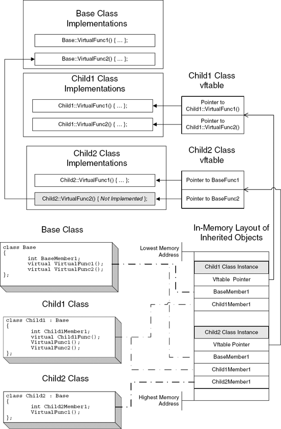
Figure C.6. In-memory layout of objects with virtual function tables. Note that this layout is more or less generic and is used by all compilers.
The revealing element here is the use of the ECX register and the fact that the CALL is not using a hard-coded address but is instead accessing a data structure in order to get the function's address. Notice that this data structure is essentially the same data structure loaded into ECX (even though it is read from a separate register, ESI). This tells you that the function pointer resides inside the object instance, which is a very strong indicator that this is indeed a virtual function call.
Let's take a look at another virtual function call, this time at one that receives some parameters.
mov      eax, DWORD PTR [esi]
push     ebx
push     edx
mov      ecx, esi
call     DWORD PTR [eax + 4]
No big news here. This sequence is identical, except that here you have two parameters that are pushed to the stack before the call is made. To summarize, identifying virtual function calls is often very easy, but it depends on the specific compiler implementation. Generally speaking, any function call sequence that loads a valid pointer into ECX and indirectly calls a function whose address is obtained via that same pointer is probably a C++ virtual member function call. This is true for code generated by the Microsoft and Intel compilers.
In code produced by other compilers such as G++ (that don't use ECX for passing the this pointer) identification might be a bit more challenging because there aren't any definite qualities that can be quickly used for determining the nature of the call. In such cases, the fact that both the function's pointer and the data it works with reside in the same data structure should be enough to convince us that we're dealing with a class. Granted, this is not always true, but if someone implemented his or her own private concept of a "class" using a generic data structure, complete with data members and function pointers stored in it, you might as well treat it as a class—it is the same thing from the low-level perspective.
For inherited objects that have virtual functions, the constructors are interesting because they perform the actual initialization of the virtual function table pointers. If you look at two constructors, one for an inherited class and another for its base class, you will see that they both initialize the object's virtual function table (even though an object only stores one virtual function table pointer). Each constructor initializes the virtual function table to its own table. This is because the constructors can't know which particular type of object was instantiated—the inherited class or the base class. Here is the constructor of a simple inherited class:
InheritedClass::InheritedClass()
push    eb
pmov    esp, eb
psub    esp, 8
mov     [ebp - 4], ebx
mov     ebx, [ebp + 8]
mov     [esp], ebx
call    BaseConstructor
mov     [ebx + 4], 0
mov     [ebx], InheritedVFTable
mov     ebx, [ebp - 4]
mov     esp, ebp
pop     ebp
ret
Notice how the constructor actually calls the base class's constructor. This is how object initialization takes place in C++. An object is initialized and the constructor for its specific type is called. If the object is inherited, the compiler adds calls to the ancestor's constructor before the beginning of the descendant's actual constructor code. The same process takes place in each ancestor's constructor until the base class is reached. Here is an example of a base class constructor:
BaseClass::BaseClass()
push      ebp
mov       ebp, esp
mov       edx, [ebp + 8]
mov       [edx], BaseVFTable
mov       [edx + 4], 0
mov       [edx + 8], 0
pop       ebp
ret
Notice how the base class sets the virtual function pointer to its own copy only to be replaced by the inherited class's constructor as soon as this function returns. Also note that this function doesn't call any other constructors since it is the base class. If you were to follow a chain of constructors where each call its parent's constructor, you would know you reached the base class at this point because this constructor doesn't call anyone else, it just initializes the virtual function table and returns.