Table of Contents for
Reversing: Secrets of Reverse Engineering
 Reversing: Secrets of Reverse Engineering
Published by
John Wiley & Sons, 2005
Reversing: Secrets of Reverse Engineering
Published by
John Wiley & Sons, 2005
- Copyright
- Credits
- Foreword
- Acknowledgments
- Introduction
- I. Reversing 101
- 1. Foundations
- 2. Low-Level Software
- 3. Windows Fundamentals
- 4. Reversing Tools
- II. Applied Reversing
- 5. Beyond the Documentation
- 6. Deciphering File Formats
- 7. Auditing Program Binaries
- 8. Reversing Malware
- III. Cracking
- 9. Piracy and Copy Protection
- 10. Antireversing Techniques
- 11. Breaking Protections
- IV. Beyond Disassembly
- 12. Reversing .NET
- 13. Decompilation
- A. Deciphering Code Structures
- B. Understanding Compiled Arithmetic
- C. Deciphering Program Data
- D. Citations
This appendix discusses the most common logical and control flow constructs used in high-level languages and demonstrates how they are implemented in IA-32 assembly language. The idea is to provide a sort of dictionary for typical assembly language sequences you are likely to run into while reversing IA-32 assembly language code.
This appendix starts off with a detailed explanation of how logic is implemented in IA-32, including how operands are compared and the various conditional codes used by the conditional branch instructions. This is followed by a detailed examination of every popular control flow construct and how it is implemented in assembly language, including loops and a variety of conditional blocks. The next section discusses branchless logic, and demonstrates the most common branchless logic sequences. Finally, I've included a brief discussion on the impact of working-set tuning on the reversing process for Windows applications.
The most basic element in software that distinguishes your average pocket calculator from a full-blown computer is the ability to execute a sequence of logical and conditional instructions. The following sections demonstrate the most common types of low-level logical constructs frequently encountered while reversing, and explain their exact meanings. I begin by going over the process of comparing two operands in assembly language, which is a significant building block used in almost every logical statement. I then proceed to discuss the conditional codes in IA-32 assembly language, which are employed in every conditional instruction in the instruction set.
The vast majority of logical statements involve the comparison of two or more operands. This is usually followed by code that can act differently based on the result of the comparison. The following sections demonstrate the operand comparison mechanism in IA-32 assembly language. This process is somewhat different for signed and unsigned operands.
The fundamental instruction for comparing operands is the CMP instruction. CMP essentially subtracts the second operand from the first and discards the result. The processor's flags are used for notifying the instructions that follow on the result of the subtraction. As with many other instructions, flags are read differently depending on whether the operands are signed or unsigned.
Note
If you're not familiar with the subtleties of IA-32 flags, it is highly recommended that you go over the "Arithmetic Flags" section in Appendix B before reading further.
Table A.1 demonstrates the behavior of the CMP instruction when comparing signed operands. Remember that the following table also applies to the SUB instruction.
Table A.1. Signed Subtraction Outcome Table for CMP and SUB (X represents the left operand, while Y represents the right operand)
LEFT OPERAND | RIGHT OPERAND | RELATION BETWEEN OPERANDS | FLAGS AFFECTED | COMMENTS |
|---|---|---|---|---|
X >= 0 | Y >= 0 | X = Y | OF=0 SF=0 ZF=1 | The two operands are equal, so the result is zero. |
X > 0 | Y >= 0 | X > Y | OF=0 SF=0 ZF=0 | Flags are all zero, indicating a positive result, with no overflow. |
X < 0 | Y < 0 | X > Y | OF=0 SF=0 ZF=0 | This is the same as the preceding case, with both X and Y containing negative integers. |
X > 0 | Y > 0 | X < Y | OF=0 SF=1 ZF=0 | An SF=1 represents a negative result, which (with OF being unset) indicates that Y is larger than X. |
X < 0 | Y >= 0 | X < Y | OF=0 SF=1 ZF=0 | This is the same as the preceding case, except that X is negative and Y is positive. Again, the combination of SF=1 with OF=0 represents that Y is greater than X. |
X < 0 | Y > 0 | X < Y | OF=1 SF=0 ZF=0 | This is another similar case where X is negative and Y is positive, except that here an overflow is generated, and the result is positive. |
X > 0 | Y < 0 | X > Y | OF=1 SF=1 ZF=0 | When X is positive and Y is a negative integer low enough to generate a positive overflow, both OF and SF are set. |
In looking at Table A.1, the ground rules for identifying the results of signed integer comparisons become clear. Here's a quick summary of the basic rules:
Anytime ZF is set you know that the subtraction resulted in a zero, which means that the operands are equal.
When all three flags are zero, you know that the first operand is greater than the second, because you have a positive result and no overflow.
When there is a negative result and no overflow (SF=1 and OF=0), you know that the second operand is larger than the first.
When there is an overflow and a positive result, the second operand must be larger than the first, because you essentially have a negative result that is too small to be represented by the destination operand (hence the overflow).
When you have an overflow and a negative result, the first operand must be larger than the second, because you essentially have a positive result that is too large to be represented by the destination operand (hence the overflow).
While it is not generally necessary to memorize the comparison outcome tables (tables A.1 and A.2), it still makes sense to go over them and make sure that you properly understand how each flag is used in the operand comparison process. This will be helpful in some cases while reversing when flags are used in unconventional ways. Knowing how flags are set during comparison and subtraction is very helpful for properly understanding logical sequences and quickly deciphering their meaning.
Table A.2 demonstrates the behavior of the CMP instruction when comparing unsigned operands. Remember that just like Table A.1, the following table also applies to the SUB instruction.
Table A.2. Unsigned Subtraction Outcome Table for CMP and SUB Instructions (X represents the left operand, while Y represents the right operand)
RELATION BETWEEN OPERANDS | FLAGS AFFECTED | COMMENTS |
|---|---|---|
x = y | CF=0 ZF=1 | The two operands are equal, so the result is zero. |
x < y | CF=1 ZF=0 | Y is larger than X so the result is lower than 0, which generates an overflow (CF=1). |
X > Y | CF=0 ZF=0 | X is larger than Y, so the result is above zero, and no overflow is generated (CF=0). |
In looking at Table A.2, the ground rules for identifying the results of unsigned integer comparisons become clear, and it's obvious that unsigned operands are easier to deal with. Here's a quick summary of the basic rules:
Anytime ZF is set you know that the subtraction resulted in a zero, which means that the operands are equal.
When both flags are zero, you know that the first operand is greater than the second, because you have a positive result and no overflow.
When you have an overflow you know that the second operand is greater than the first, because the result must be too low in order to be represented by the destination operand.
Conditional codes are suffixes added to certain conditional instructions in order to define the conditions governing their execution.
It is important for reversers to understand these mnemonics because virtually every conditional code sequence will include one or more of them. Sometimes their meaning will be very intuitive—take a look at the following code:
cmp
eax, 7
je
SomePlace
In this example, it is obvious that JE (which is jump if equal) will cause a jump to SomePlace if EAX equals 7. This is one of the more obvious cases where understanding the specifics of instructions such as CMP and of the conditional codes is really unnecessary. Unfortunately for us reversers, there are quite a few cases where the conditional codes are used in unintuitive ways. Understanding how the conditional codes use the flags is important for properly understanding program logic. The following sections list each condition code and explain which flags it uses and why.
Note
The conditional codes listed in the following sections are listed as standalone codes, even though they are normally used as instruction suffixes to conditional instructions. Conditional codes are never used alone.
Table A.3 presents the IA-32 conditional codes defined for signed operands. Note that in all signed conditional codes overflows are detected using the overflow flag (OF). This is because the arithmetic instructions use OF for indicating signed overflows.
Table A.3. Signed Conditional Codes Table for CMPP and SUB
MNEMONICS | FLAGS | SATISFIED WHEN | COMMENTS |
|---|---|---|---|
If Greater (G) If Not Less or Equal (NLE) | ZF=0 AND ((OF=0 AND SF=0) OR (OF=1 AND SF=1)) | x > y | Use ZF to confirm that the operands are unequal. Also use SF to check for either a positive result without an overflow, indicating that the first operand is greater, or a negative result with an overflow. The latter would indicate that the second operand was a low enough negative integer to produce a result too large to be represented by the destination (hence the overflow). |
If Greater or Equal(GE) If Not Less (NL) | (OF=0 AND SF=0) OR (OF=1 AND SF=1) | x >= Y | This code is similar to the preceding code with the exception that it doesn't check ZF for zero, so it would also be satisfied by equal operands. |
If Less (L) If Not Greater or Equal (NGE) | (OF=1 AND SF=0) OR (OF=0 AND SF=1) | X < Y | Check for OF=1 AND SF=0 indicating that X was lower than Y and the result was too low to be represented by the destination operand (you got an overflow and a positive result). The other case is OF=0 AND SF=1. This is a similar case, except that no overflow is generated, and the result is negative. |
If Less or Equal (LE) If Not Greater (NG) | ZF=1 OR ((OF=1 AND SF=0) OR (OF=0 AND SF=1)) | X <= Y | This code is the same as the preceding code with the exception that it also checks ZF and so would also be satisfied if the operands are equal. |
Table A.4 presents the IA-32 conditional codes defined for unsigned operands. Note that in all unsigned conditional codes, overflows are detected using the carry flag (CF). This is because the arithmetic instructions use CF for indicating unsigned overflows.
Table A.4. Unsigned Conditional Codes
MNEMONICS | FLAGS | SATISFIED WHEN | COMMENTS |
|---|---|---|---|
If Above (A) If Not Below or Equal (NBE) | CF=0 AND ZF=0 | X > Y | Use CF to confirm that the second operand is not larger than the first (because then CF would be set), and ZF to confirm that the operands are unequal. |
If Above or Equal (AE) If Not Below (NB) If Not Carry (NC) | CF = 0 | X >= Y | This code is similar to the above with the exception that it only checks CF, so it would also be satisfied by equal operands. |
If Below (B) If Not Above or Equal (NAE) If Carry (C) | CF=1 | X < Y | When CF is set we know that the second operand is greater than the first because an overflow could only mean that the result was negative. |
CF=1 OR ZF=1 | X <= Y | This code is the same as the above with the exception that it also checks ZF, and so would also be satisfied if the operands are equal. | |
If Equal (E) If Zero (Z) | ZF=1 | X = Y | ZF is set so we know that the result was zero, meaning that the operands are equal. |
If Not Equal (NE) If Not Zero (NZ) | ZF=0 | Z != Y | ZF is unset so we know that the result was nonzero, which implies that the operands are unequal. |
The vast majority of logic in the average computer program is implemented through branches. These are the most common programming constructs, regardless of the high-level language. A program tests one or more logical conditions, and branches to a different part of the program based on the result of the logical test. Identifying branches and figuring out their meaning and purpose is one of the most basic code-level reversing tasks.
The following sections introduce the most popular control flow constructs and program layout elements. I start with a discussion of procedures and how they are represented in assembly language and proceed to a discussion of the most common control flow constructs and to a comparison of their low-level representations with their high-level representations. The constructs discussed are single branch conditionals, two-way conditionals, n-way conditionals, and loops, among others.
The most basic building block in a program is the procedure, or function. From a reversing standpoint functions are very easy to detect because of function prologues and epilogues. These are standard initialization sequences that compilers generate for nearly every function. The particulars of these sequences depend on the specific compiler used and on other issues such as calling convention. Calling conventions are discussed in the section on calling conventions in Appendix C.
On IA-32 processors function are nearly always called using the CALL instruction, which stores the current instruction pointer in the stack and jumps to the function address. This makes it easy to distinguish function calls from other unconditional jumps.
Internal functions are called from the same binary executable that contains their implementation. When compilers generate an internal function call sequence they usually just embed the function's address into the code, which makes it very easy to detect. The following is a common internal function call.
Call CodeSectionAddress
An imported function call takes place when a module is making a call into a function implemented in another binary executable. This is important because during the compilation process the compiler has no idea where the imported function can be found and is therefore unable to embed the function's address into the code (as is usually done with internal functions).
Imported function calls are implemented using the Import Directory and Import Address Table (see Chapter 3). The import directory is used in runtime for resolving the function's name with a matching function in the target executable, and the IAT stores the actual address of the target function. The caller then loads the function's pointer from the IAT and calls it. The following is an example of a typical imported function call:
call DWORD PTR [IAT_Pointer]
Notice the DWORD PTR that precedes the pointer—it is important because it tells the CPU to jump not to the address of IAT_Pointer but to the address that is pointed to by IAT_Pointer. Also keep in mind that the pointer will usually not be named (depending on the disassembler) and will simply contain an address pointing into the IAT.
Detecting imported calls is easy because except for these types of calls, functions are rarely called indirectly through a hard-coded function pointer. I would, however, recommend that you determine the location of the IAT early on in reversing sessions and use it to confirm that a function is indeed imported. Locating the IAT is quite easy and can be done with a variety of different tools that dump the module's PE header and provide the address of the IAT. Tools for dumping PE headers are discussed in Chapter 4.
Some disassemblers and debuggers will automatically indicate an imported function call (by internally checking the IAT address), thus saving you the trouble.
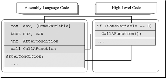
The most basic form of logic in most programs consists of a condition and an ensuing conditional branch. In high-level languages, this is written as an if statement with a condition and a block of conditional code that gets executed if the condition is satisfied. Here's a quick sample:
if (SomeVariable == 0)
     CallAFunction();
From a low-level perspective, implementing this statement requires a logical check to determine whether SomeVariable contains 0 or not, followed by code that skips the conditional block by performing a conditional jump if SomeVariable is nonzero. Figure A.1 depicts how this code snippet would typically map into assembly language.
The assembly language code in Figure A.1 uses TEST to perform a simple zero check for EAX. TEST works by performing a bitwise AND operation on EAX and setting flags to reflect the result (the actual result is discarded). This is an effective way to test whether EAX is zero or nonzero because TEST sets the zero flag (ZF) according to the result of the bitwise AND operation. Note that the condition is reversed: In the source code, the program was checking whether SomeVariable equals zero, but the compiler reversed the condition so that the conditional instruction (in this case a jump) checks whether SomeVariable is nonzero. This stems from the fact that the compiler-generated binary code is organized in memory in the same order as it is organized in the source code. Therefore if SomeVariable is nonzero, the compiler must skip the conditional code section and go straight to the code section that follows.
The bottom line is that in single-branch conditionals you must always reverse the meaning of the conditional jump in order to obtain the true high-level logical intention.
Another fundamental functionality of high-level languages is to allow the use of two-way conditionals, typically implemented in high-level languages using the if-else keyword pair. A two-way conditional is different from a single-branch conditional in the sense that if the condition is not satisfied, the program executes an alternative code block and only then proceeds to the code that follows the 'if-else' statement. These constructs are called two-way conditionals because the flow of the program is split into one of two different possible paths: the one in the 'if' block, or the one in the 'else' block.
Let's take a quick look at how compilers implement two-way conditionals. First of all, in two-way conditionals the conditional branch points to the 'else' block and not to the code that follows the conditional statement. Second, the condition itself is almost always reversed (so that the jump to the 'else' block only takes place when the condition is not satisfied), and the primary conditional block is placed right after the conditional jump (so that the conditional code gets executed if the condition is satisfied). The conditional block always ends with an unconditional jump that essentially skips the 'else' block—this is a good indicator for identifying two-way conditionals. The 'else' block is placed at the end of the conditional block, right after that unconditional jump. Figure A.2 shows what an average if-else statement looks like in assembly language.
Notice the unconditional JMP right after the function call. That is where the first condition skips the else block and jumps to the code that follows. The basic pattern to look for when trying to detect a simple 'if-else' statement in a disassembled program is a condition where the code that follows it ends with an unconditional jump.
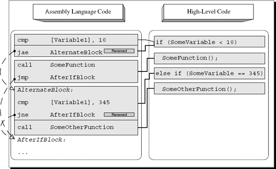
Most high-level languages also support a slightly more complex version of a two-way conditional where a separate conditional statement is used for each of the two code blocks. This is usually implemented by combining the 'if' and else-if keywords where each statement is used with a separate conditional statement. This way, if the first condition is not satisfied, the program jumps to the second condition, evaluates that one, and simply skips the entire conditional block if neither condition is satisfied. If one of the conditions is satisfied, the corresponding conditional block is executed, and execution just flows into the next program statement. Figure A.3 provides a high-level/low-level view of this type of control flow construct.
Sometimes programmers create long statements with multiple conditions, where each condition leads to the execution of a different code block. One way to implement this in high-level languages is by using a "switch" block (discussed later), but it is also possible to do this using conventional 'if' statements. The reason that programmers sometimes must use 'if' statements is that they allow for more flexible conditional statements. The problem is that 'switch' blocks don't support complex conditions, only the use of hard-coded constants. In contrast, a sequence of 'else-if' statements allows for any kind of complex condition on each of the blocks—it is just more flexible.
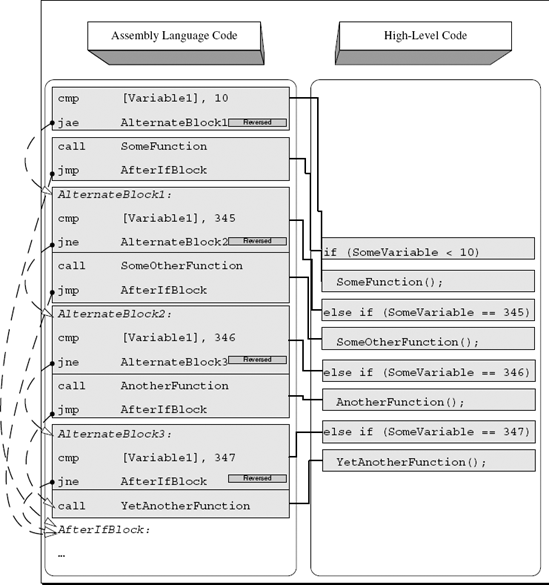
The guidelines for identifying such blocks are very similar to the ones used for plain two-way conditionals in the previous section. The difference here is that the compiler adds additional "alternate blocks" that consist of one or more logical checks, the actual conditional code block, and the final JMP that skips to the end of the entire block. Of course, the JMP only gets executed if the condition is satisfied. Unlike 'switch' blocks where several conditions can lead to the same code block, with these kinds of 'else-if' blocks each condition is linked to just one code block. Figure A.4 demonstrates a four-way conditional sequence with one 'if' and three alternate 'else-if' paths that follow.
In real-life, programs often use conditional statements that are based on more than just a single condition. It is very common to check two or more conditions in order to decide whether to enter a conditional code block or not. This slightly complicates things for reversers because the low-level code generated for a combination of logical checks is not always easy to decipher. The following sections demonstrate typical compound conditionals and how they are deciphered. I will begin by briefly discussing the most common logical operators used for constructing compound conditionals and proceed to demonstrate several different compound conditionals from both the low-level and the high-level perspectives.
High-level languages have special operators that allow the use of compound conditionals in a single conditional statement. When specifying more than one condition, the code must specify how the multiple conditions are to be combined.
The two most common operators for combining more than one logical statements are AND and OR (not to be confused with the bitwise logic operators).
As the name implies, AND (denoted as && in C and C++) denotes that two statements must be satisfied for the condition to be considered true. Detecting such code in assembly language is usually very easy, because you will see two consecutive conditions that conditionally branch to the same address. Here is an example:
cmp      [Variable1], 100
jne      AfterCondition
cmp      [Variable2], 50
jne      AfterCondition
ret
AfterCondition:
.
.
.
In this snippet, the revealing element is the fact that both conditional jumps point to the same address in the code (AfterCondition). The idea is simple: Check the first condition, and skip to end of the conditional block if not met. If the first condition is met, proceed to test the second condition and again, skip to the end of the conditional block if it is not met. The conditional code block is placed right after the second conditional branch (so that if neither branch is taken you immediately proceed to execute the conditional code block). Deciphering the actual conditions is the same as in a single statement condition, meaning that they are also reversed. In this case, testing that Variable1 doesn't equal 100 means that the original code checked whether Variable1 equals 100. Based on this information you can reconstruct the source code for this snippet:
if (Variable1 == 100 && Variable2 == 50)
                                                           return;
Figure A.5 demonstrates how the above high-level code maps to the assembly language code presented earlier.
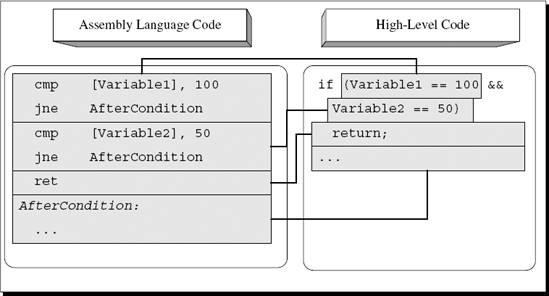
Figure A.5. High-level/low-level view of a compound conditional statement with two conditions combined using the AND operator.
Another common logical operator is the OR operator, which is used for creating conditional statements that only require for one of the conditions specified to be satisfied. The OR operator means that the conditional statement is considered to be satisfied if either the first condition or the second condition is true. In C and C++, OR operators are denoted using the || symbol. Detecting conditional statements containing OR operators while reversing is slightly more complicated than detecting AND operators. The straightforward approach for implementing the OR operator is to use a conditional jump for each condition (without reversing the conditions) and add a final jump that skips the conditional code block if neither conditions are met. Here is an example of this strategy:
cmp               [Variable1], 100
je                ConditionalBlock
cmp               [Variable2], 50
je                ConditionalBlock
jmp               AfterConditionalBlock
ConditionalBlock:
call  SomeFunction
AfterConditionalBlock:
.
.
.
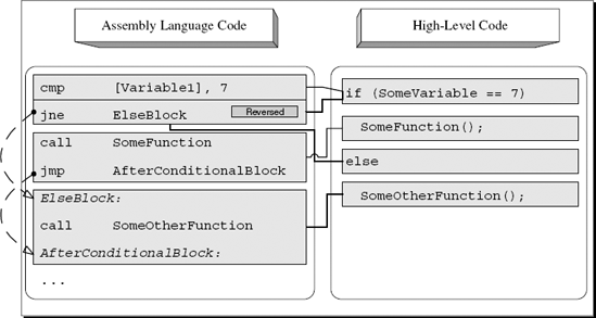
Figure A.6 demonstrates how the preceding snippet maps into the original source code.
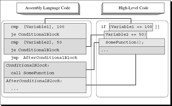
Figure A.6. High-level/low-level view of a compound conditional statement with two conditions combined using the OR operator.
Again, the most noticeable element in this snippet is the sequence of conditional jumps all pointing to the same code. Keep in mind that with this approach the conditional jumps actually point to the conditional block (as opposed to the previous cases that have been discussed, where conditional jumps point to the code that follows the conditional blocks). This approach is employed by GCC and several other compilers and has the advantage (at least from a reversing perspective) of being fairly readable and intuitive. It does have a minor performance disadvantage because of that final JMP that's reached when neither condition is met.
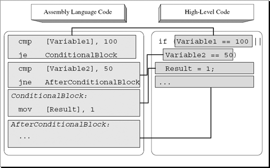
Other optimizing compilers such as the Microsoft compilers get around this problem of having an extra JMP by employing a slightly different approach for implementing the OR operator. The idea is that only the second condition is reversed and is pointed at the code after the conditional block, while the first condition still points to the conditional block itself. Figure A.7 illustrates what the same logic looks like when compiled using this approach.
The first condition checks whether Variable1 equals 100, just as it's stated in the source code. The second condition has been reversed and is now checking whether Variable2 doesn't equal 50. This is so because you want the first condition to jump to the conditional code if the condition is met and the second condition to not jump if the (reversed) condition is met. The second condition skips the conditional block when it is not met.
What happens when any of the logical operators are used to specify more than two conditions? Usually it is just a straightforward extension of the strategy employed for two conditions. For GCC this simply means another condition before the unconditional jump.
In the snippet shown in Figure A.8, Variable1 and Variable2 are compared against the same values as in the original sample, except that here we also have Variable3 which is compared against 0. As long as all conditions are connected using an OR operator, the compiler will simply add extra conditional jumps that go to the conditional block. Again, the compiler will always place an unconditional jump right after the final conditional branch instruction. This unconditional jump will skip the conditional block and go directly to the code that follows it if none of the conditions are satisfied.
With the more optimized technique, the approach is the same, except that instead of using an unconditional jump, the last condition is reversed. The rest of the conditions are implemented as straight conditional jumps that point to the conditional code block. Figure A.9 shows what happens when the same code sample from Figure A.8 is compiled using the second technique.
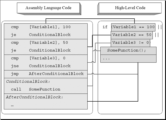
Figure A.8. High-level/low-level view of a compound conditional statement with three conditions combined using the OR operator.
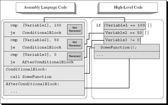
Figure A.9. High-level/low-level view of a conditional statement with three conditions combined using a more efficient version of the OR operator.
The idea is simple. When multiple OR operators are used, the compiler will produce multiple consecutive conditional jumps that each go to the conditional block if they are satisfied. The last condition will be reversed and will jump to the code right after the conditional block so that if the condition is met the jump won't occur and execution will proceed to the conditional block that resides right after that last conditional jump. In the preceding sample, the final check checks that Variable3 doesn't equal zero, which is why it uses JE.
Let's now take a look at what happens when more than two conditions are combined using the AND operator (see Figure A.10). In this case, the compiler simply adds more and more reversed conditions that skip the conditional block if satisfied (keep in mind that the conditions are reversed) and continue to the next condition (or to the conditional block itself) if not satisfied.
High-level programming languages allow programmers to combine any number of conditions using the logical operators. This means that programmers can create complex combinations of conditional statements all combined using the logical operators.
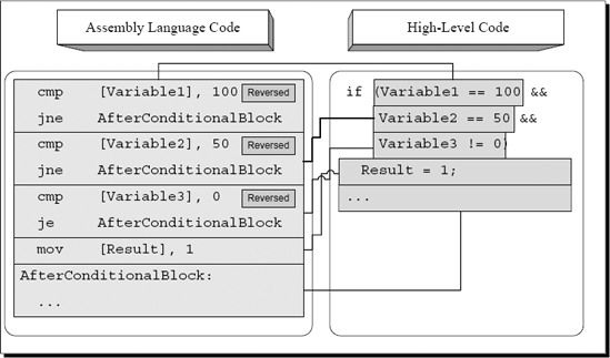
Figure A.10. High-level/low-level view of a compound conditional statement with three conditions combined using the AND operator.
There are quite a few different combinations that programmers could use, and I could never possibly cover every one of those combinations. Instead, let's take a quick look at one combination and try and determine the general rules for properly deciphering these kinds of statements.
cmp                          [Variable1], 100
je                           ConditionalBlock
cmp                           [Variable2], 50
jne                     AfterConditionalBlock
cmp                            [Variable3], 0
je                      AfterConditionalBlock
ConditionalBlock:
call                             SomeFunction
AfterConditionalBlock:
.
.
.
This sample is identical to the previous sample of an optimized application of the OR logical operator, except that an additional condition has been added to test whether Variable3 equals zero. If it is, the conditional code block is not executed. The following C code is a high-level representation of the preceding assembly language snippet.
if (Variable1 == 100 || (Variable2 == 50 && Variable3 != 0))
SomeFunction();
It is not easy to define truly generic rules for reading compound conditionals in assembly language, but the basic parameter to look for is the jump target address of each one of the conditional branches. Conditions combined using the OR operator will usually jump directly to the conditional code block, and their conditions will not be reversed (except for the last condition, which will point to the code that follows the conditional block and will be reversed). In contrast, conditions combined using the AND operator will tend to be reversed and jump to the code block that follows the conditional code block. When analyzing complex compound conditionals, you must simply use these basic rules to try and figure out each condition and see how the conditions are connected.
Switch blocks (or n-way conditionals) are commonly used when different behavior is required for different values all coming from the same operand. Switch blocks essentially let programmers create tables of possible values and responses. Note that usually a single response can be used for more than one value.
Compilers have several methods for dealing with switch blocks, depending on how large they are and what range of values they accept. The following sections demonstrate the two most common implementations of n-way conditionals: the table implementation and the tree implementation.
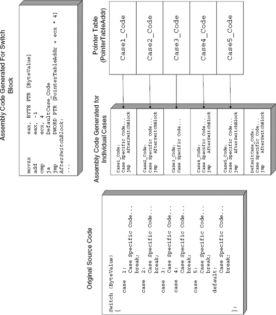
The most efficient approach (from a runtime performance standpoint) for large switch blocks is to generate a pointer table. The idea is to compile each of the code blocks in the switch statement, and to record the pointers to each one of those code blocks in a table. Later, when the switch block is executed, the operand on which the switch block operates is used as an index into that pointer table, and the processor simply jumps to the correct code block. Note that this is not a function call, but rather an unconditional jump that goes through a pointer table.
The pointer tables are usually placed right after the function that contains the switch block, but that's not always the case—it depends on the specific compiler used. When a function table is placed in the middle of the code section, you pretty much know for a fact that it is a 'switch' block pointer table. Hard-coded pointer tables within the code section aren't really a common sight.
Figure A.11 demonstrates how an n-way conditional is implemented using a table. The first case constant in the source code is 1 and the last is 5, so there are essentially five different case blocks to be supported in the table. The default block is not implemented as part of the table because there is no specific value that triggers it—any value that's not within the 1–5 range will make the program jump to the default block. To efficiently implement the table lookup, the compiler subtracts 1 from ByteValue and compares it to 4. If ByteValue is above 4, the compiler unconditionally jumps to the default case. Otherwise, the compiler proceeds directly to the unconditional JMP that calls the specific conditional block. This JMP is the unique thing about table-based n-way conditionals, and it really makes it easy to identify them while reversing. Instead of using an immediate, hard-coded address like pretty much every other unconditional jump you'll run into, this type of JMP uses a dynamically calculated memory address (usually bracketed in the disassembly) to obtain the target address (this is essentially the table lookup operation).
When you look at the code for each conditional block, notice how each of the conditional cases ends with an unconditional JMP that jumps back to the code that follows the switch block. One exception is case #3, which doesn't terminate with a break instruction. This means that when this case is executed, execution will flow directly into case 4. This works smoothly in the table implementation because the compiler places the individual cases sequentially into memory. The code for case number 4 is always positioned right after case 3, so the compiler simply avoids the unconditional JMP.
When conditions aren't right for applying the table implementation for switch blocks, the compiler implements a binary tree search strategy to reach the desired item as quickly as possible. Binary tree searches are a common concept in computer science.
The general idea is to divide the searchable items into two equally sized groups based on their values and record the range of values contained in each group. The process is then repeated for each of the smaller groups until the individual items are reached. While searching you start with the two large groups and check which one contains the correct range of values (indicating that it would contain your item). You then check the internal division within that group and determine which subgroup contains your item, and so on and so forth until you reach the correct item.
To implement a binary search for switch blocks, the compiler must internally represent the switch block as a tree. The idea is that instead of comparing the provided value against each one of the possible cases in runtime, the compiler generates code that first checks whether the provided value is within the first or second group. The compiler then jumps to another code section that checks the value against the values accepted within the smaller subgroup. This process continues until the correct item is found or until the conditional block is exited (if no case block is found for the value being searched).
Let's take a look at a common switch block implemented in C and observe how it is transformed into a tree by the compiler.
switch (Value)
{
     case 120:
            Code...
            break;
     case 140:
            Code...
            break;
     case 501:
            Code...
            break;
     case 1001:
            Code...
            break;
     case 1100:
            Code...
            break;
     case 1400:
            Code...
            break;
     case 2000:
            Code...
            break;
     case 3400:
            Code...
            break;
     case 4100:
            Code...
            break;
};
Figure A.12 demonstrates how the preceding switch block can be viewed as a tree by the compiler and presents the compiler-generated assembly code that implements each tree node.
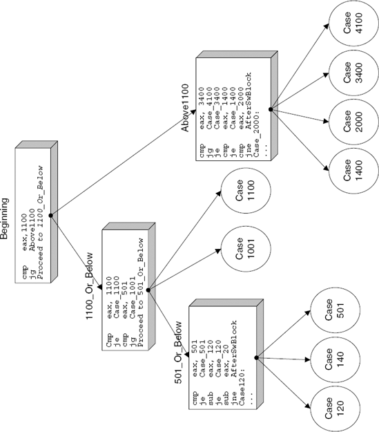
One relatively unusual quality of tree-based n-way conditionals that makes them a bit easier to make out while reading disassembled code is the numerous subtractions often performed on a single register. These subtractions are usually followed by conditional jumps that lead to the specific case blocks (this layout can be clearly seen in the 501_Or_Below case in Figure A.12). The compiler typically starts with the original value passed to the conditional block and gradually subtracts certain values from it (these are usually the case block values), constantly checking if the result is zero. This is simply an efficient way to determine which case block to jump into using the smallest possible code.
When you think about it, a loop is merely a chunk of conditional code just like the ones discussed earlier, with the difference that it is repeatedly executed, usually until the condition is no longer satisfied. Loops typically (but not always) include a counter of some sort that is used to control the number of iterations left to go before the loop is terminated. Fundamentally, loops in any high-level language can be divided into two categories, pretested loops, which contain logic followed by the loop's body (that's the code that will be repeatedly executed) and posttested loops, which contain the loop body followed by the logic.
Let's take a look at the various types of loops and examine how they are represented in assembly language,
Pretested loops are probably the most popular loop construct, even though they are slightly less efficient compared to posttested ones. The problem is that to represent a pretested loop the assembly language code must contain two jump instructions: a conditional branch instruction in the beginning (that will terminate the loop when the condition is no longer satisfied) and an unconditional jump at the end that jumps back to the beginning of the loop. Let's take a look at a simple pretested loop and see how it is implemented by the compiler:
c = 0;
while (c < 1000)
{
    array[c] = c;
    c++;
}
You can easily see that this is a pretested loop, because the loop first checks that c is lower than 1,000 and then performs the loop's body. Here is the assembly language code most compilers would generate from the preceding code:
mov              ecx, DWORD PTR [array]
xor              eax, eax
LoopStart:
mov              DWORD PTR [ecx+eax*4], eax
add              eax, 1
cmp              eax, 1000
jl               LoopStart
It appears that even though the condition in the source code was located before the loop, the compiler saw fit to relocate it. The reason that this happens is that testing the counter after the loop provides a (relatively minor) performance improvement. As I've explained, converting this loop to a posttested one means that the compiler can eliminate the unconditional JMP instruction at the end of the loop.
There is one potential risk with this implementation. What happens if the counter starts out at an out-of-bounds value? That could cause problems because the loop body uses the loop counter for accessing an array. The programmer was expecting that the counter be tested before running the loop body, not after! The reason that this is not a problem in this particular case is that the counter is explicitly initialized to zero before the loop starts, so the compiler knows that it is zero and that there's nothing to check. If the counter were to come from an unknown source (as a parameter passed from some other, unknown function for instance), the compiler would probably place the logic where it belongs: in the beginning of the sequence.
Let's try this out by changing the above C loop to take the value of counter c from an external source, and recompile this sequence. The following is the output from the Microsoft compiler in this case:
mov           eax, DWORD PTR [c]
mov           ecx, DWORD PTR [array]
cmp           eax, 1000
jge           EndOfLoop
LoopStart:
mov           DWORD PTR [ecx+eax*4], eax
add           eax, 1
cmp           eax, 1000
jl            LoopStart
EndOfLoop:
It seems that even in this case the compiler is intent on avoiding the two jumps. Instead of moving the comparison to the beginning of the loop and adding an unconditional jump at the end, the compiler leaves everything as it is and simply adds another condition at the beginning of the loop. This initial check (which only gets executed once) will make sure that the loop is not entered if the counter has an illegal value. The rest of the loop remains the same.
So what kind of an effect do posttested loops implemented in the high-level realm actually have on the resulting assembly language code if the compiler produces posttested sequences anyway? Unsurprisingly—very little.
When a program contains a do...while() loop, the compiler generates a very similar sequence to the one in the previous section. The only difference is that with do...while() loops the compiler never has to worry about whether the loop's conditional statement is expected to be satisfied or not in the first run. It is placed at the end of the loop anyway, so it must be tested anyway. Unlike the previous case where changing the starting value of the counter to an unknown value made the compiler add another check before the beginning of the loop, with do...while() it just isn't necessary. This means that with posttested loops the logic is always placed after the loop's body, the same way it's arranged in the source code.
A loop break condition occurs when code inside the loop's body terminates the loop (in C and C++ this is done using the break keyword). The break keyword simply interrupts the loop and jumps to the code that follows. The following assembly code is the same loop you've looked at before with a conditional break statement added to it:
mov          eax, DWORD PTR [c]
mov          ecx, DWORD PTR [array]
LoopStart:
cmp          DWORD PTR [ecx+eax*4], 0
jne          AfterLoop
mov          DWORD PTR [ecx+eax*4], eax
add          eax, 1
cmp          eax, 1000
jl           LoopStart
AfterLoop:
This code is slightly different from the one in the previous examples because even though the counter originates in an unknown source the condition is only checked at the end of the loop. This is indicative of a posttested loop. Also, a new check has been added that checks the current array item before it is initialized and jumps to AfterLoop if it is nonzero. This is your break statement—simply an elegant name for the good old goto command that was so popular in "lesser" programming languages.
For this you can easily deduce the original source to be somewhat similar to the following:
do
{
    if (array[c])
        break;

        array[c] = c;
    c++;
} while (c < 1000);A loop skip-cycle statement is implemented in C and C++ using the continue keyword. The statement skips the current iteration of the loop and jumps straight to the loop's conditional statement, which decides whether to perform another iteration or just exit the loop. Depending on the specific type of the loop, the counter (if one is used) is usually not incremented because the code that increments it is skipped along with the rest of the loop's body. This is one place where for loops differ from while loops. In for loops, the code that increments the counter is considered part of the loop's logical statement, which is why continue doesn't skip the counter increment in such loops. Let's take a look at a compiler-generated assembly language snippet for a loop that has a skip-cycle statement in it:
mov            eax, DWORD PTR [c]
mov            ecx, DWORD PTR [array]
LoopStart:
cmp            DWORD PTR [ecx+eax*4], 0
jne            NextCyclemov DWORD PTR [ecx+eax*4], eax
add            eax, 1
NextCycle:
cmp            eax, 1000
jl             SHORT LoopStart
This code sample is the same loop you've been looking at except that the condition now invokes the continue command instead of the break command. Notice how the condition jumps to NextCycle and skips the incrementing of the counter. The program then checks the counter's value and jumps back to the beginning of the loop if the counter is lower than 1,000.
Here is the same code with a slight modification:
mov          eax, DWORD PTR [c]
mov          ecx, DWORD PTR [array]
LoopStart:
cmp          DWORD PTR [ecx+eax*4], 0
jne          NextCycle
mov          DWORD PTR [ecx+eax*4], eax
NextCycle:
add          eax, 1
cmp          eax, 1000
jl           SHORT LoopStart
The only difference here is that NextCycle is now placed earlier, before the counter-incrementing code. This means that unlike before, the continue statement will increment the counter and run the loop's logic. This indicates that the loop was probably implemented using the for keyword. Another way of implementing this type of sequence without using a for loop is by using a while or do...while loop and incrementing the counter inside the conditional statement, using the ++ operator. In this case, the logical statement would look like this:
do { ... } while (++c < 1000);Loop unrolling is a code-shaping level optimization that is not CPU- or instruction-set-specific, which means that it is essentially a restructuring of the high-level code aimed at producing more efficient machine code. The following is an assembly language example of a partially unrolled loop:
xor         ecx,ecx
pop         ebx
lea         ecx,[ecx]
LoopStart:
mov         edx,dword ptr [esp+ecx*4+8]
add         edx,dword ptr [esp+ecx*4+4]
add         ecx,3
add         edx,dword ptr [esp+ecx*4-0Ch]
add         eax,edx
cmp         ecx,3E7h
jl          LoopStart
This loop is clearly a partially unrolled loop, and the best indicator that this is the case is the fact that the counter is incremented by three in each iteration. Essentially what the compiler has done is it duplicated the loop's body three times, so that each iteration actually performs the work of three iterations instead of one. The counter incrementing code has been corrected to increment by 3 instead of 1 in each iteration. This is more efficient because the loop's overhead is greatly reduced—instead of executing the CMP and JL instructions 0x3e7 (999) times, they will only be executed 0x14d (333) times.
A more aggressive type of loop unrolling is to simply eliminate the loop altogether and actually duplicate its body as many times as needed. Depending on the number of iterations (and assuming that number is known in advance), this may or may not be a practical approach.
Some optimizing compilers have special optimization techniques for generating branchless logic. The main goal behind all of these techniques is to eliminate or at least reduce the number of conditional jumps required for implementing a given logical statement. The reasons for wanting to reduce the number of jumps in the code to the absolute minimum is explained in the section titled "Hardware Execution Environments in Modern Processors" in Chapter 2. Briefly, the use of a processor pipeline dictates that when the processor encounters a conditional jump, it must guess or predict whether the jump will take place or not, and based on that guess decide which instructions to add to the end of the pipeline—the ones that immediately follow the branch or the ones at the jump's target address. If it guesses wrong, the entire pipeline is emptied and must be refilled. The amount of time wasted in these situations heavily depends on the processor's internal design and primarily on its pipeline length, but in most pipelined CPUs refilling the pipeline is a highly expensive operation.
Some compilers implement special optimizations that use sophisticated arithmetic and conditional instructions to eliminate or reduce the number of jumps required in order to implement logic. These optimizations are usually applied to code that conditionally performs one or more arithmetic or assignment operations on operands. The idea is to convert the two or more conditional execution paths into a single sequence of arithmetic operations that result in the same data, but without the need for conditional jumps.
There are two major types of branchless logic code emitted by popular compilers. One is based on converting logic into a purely arithmetic sequence that provides the same end result as the original high-level language logic. This technique is very limited and can only be applied to relatively simple sequences. For slightly more involved logical statements, compilers sometimes employ special conditional instructions (when available on the target CPU). The two primary approaches for implementing branchless logic are discussed in the following sections.
Certain logical statements can be converted directly into a series of arithmetic operations, involving no conditional execution whatsoever. These are elegant mathematical tricks that allow compilers to translate branched logic in the source code into a simple sequence of arithmetic operations. Consider the following code:
mov      eax, [ebp - 10]
and      eax, 0x00001000
neg      eax
sbb      eax, eax
neg      eax
ret
The preceding compiler-generated code snippet is quite common in IA-32 programs, and many reversers have a hard time deciphering its meaning. Considering the popularity of these sequences, you should go over this sample and make sure you understand how it works.
The code starts out with a simple logical AND of a local variable with 0x00001000, storing the result into EAX (the AND instruction always sends the result to the first, left-hand operand). You then proceed to a NEG instruction, which is slightly less common. NEG is a simple negation instruction, which reverses the sign of the operand—this is sometimes called two's complement. Mathematically, NEG performs a simple
Result = -(Operand);
operation. The interesting part of this sequence is the SBB instruction. SBB is a subtraction with borrow instruction. This means that SBB takes the second (right-hand) operand and adds the value of CF to it and then subtracts the result from the first operand. Here's a pseudocode for SBB:
Operand1 = Operand1 – (Operand2 + CF);
Notice that in the preceding sample SBB was used on a single operand. This means that SBB will essentially subtract EAX from itself, which of course is a mathematically meaningless operation if you disregard CF. Because CF is added to the second operand, the result will depend solely on the value of CF. If CF == 1, EAX will become −1. If CF == 0, EAX will become zero. It should be obvious that the value of EAX after the first NEG was irrelevant. It is immediately lost in the following SBB because it subtracts EAX from itself. This raises the question of why did the compiler even bother with the NEG instruction?
The Intel documentation states that beyond reversing the operand's sign, NEG will also set the value of CF based on the value of the operand. If the operand is zero when NEG is executed, CF will be set to zero. If the operand is nonzero, CF will be set to one. It appears that some compilers like to use this additional functionality provided by NEG as a clever way to check whether an operand contains a zero or nonzero value. Let's quickly go over each step in this sequence:
Use
NEGto check whether the source operand is zero or nonzero. The result is stored in CF.Use
SBBto transfer the result from CF back to a usable register. Of course, because of the nature ofSBB, a nonzero value in CF will become −1 rather than 1. Whether that's a problem or not depends on the nature of the high-level language. Some languages use 1 to denote True, while others use −1.Because the code in the sample came from a C/C++ compiler, which uses 1 to denote True, an additional
NEGis required, except that this timeNEGis actually employed for reversing the operand's sign. If the operand is −1, it will become 1. If it's zero it will of course remain zero.
The following is a pseudocode that will help clarify the steps described previously:
EAX = EAX & 0x00001000;
if (EAX)
     CF = 1;
else
     CF = 0;

EAX = EAX - (EAX + CF);
EAX = -EAX;
Essentially, what this sequence does is check for a particular bit in EAX (0x00001000), and returns 1 if it is set or zero if it isn't. It is quite elegant in the sense that it is purely arithmetic—there are no conditional branch instructions involved. Let's quickly translate this sequence back into a high-level C representation:
if (LocalVariable & 0x00001000)
                                      return TRUE;
else
return FALSE;
That's much more readable, isn't it? Still, as reversers we're often forced to work with such less readable, unattractive code sequences as the one just dissected. Knowing and understanding these types of low-level tricks is very helpful because they are very frequently used in compiler-generated code.
Let's take a look at another, slightly more involved, example of how high-level logical constructs can be implemented using pure arithmetic:
call      SomeFunc
sub       eax, 4
neg       eax
sbb       eax, eax
and       al, −52
add       eax, 54
ret
You'll notice that this sequence also uses the NEG/SBB combination, except that this one has somewhat more complex functionality. The sequence starts by calling a function and subtracting 4 from its return value. It then invokes NEG and SBB in order to perform a zero test on the result, just as you saw in the previous example. If after the subtraction the return value from SomeFunc is zero, SBB will set EAX to zero. If the subtracted return value is nonzero, SBB will set EAX to −1 (or 0xffffffff in hexadecimal).
The next two instructions are the clever part of this sequence. Let's start by looking at that AND instruction. Because SBB is going to set EAX either to zero or to 0xffffffff, we can consider the following AND instruction to be similar to a conditional assignment instruction (much like the CMOV instruction discussed later). By ANDing EAX with a constant, the code is essentially saying: "if the result from SBB is zero, do nothing. If the result is −1, set EAX to the specified constant." After doing this, the code unconditionally adds 54 to EAX and returns to the caller.
The challenge at this point is to try and figure out what this all means. This sequence is obviously performing some kind of transformation on the return value of SomeFunc and returning that transformed value to the caller. Let's try and analyze the bottom line of this sequence. It looks like the return value is going to be one of two values: If the outcome of SBB is zero (which means that SomeFunc's return value was 4), EAX will be set to 54. If SBB produces 0xffffffff, EAX will be set to 2, because the AND instruction will set it to −52, and the ADD instruction will bring the value up to 2.
This is a sequence that compares a pair of integers, and produces (without the use of any branches) one value if the two integers are equal and another value if they are unequal. The following is a C version of the assembly language snippet from earlier:
if (SomeFunc() == 4)
     return 54;
else
return 2;Using arithmetic sequences to implement branchless logic is a very limited technique. For more elaborate branchless logic, compilers employ conditional instructions (provided that such instructions are available on the target CPU architecture). The idea behind conditional instructions is that instead of having to branch to two different code sections, compilers can sometimes use special instructions that are only executed if certain conditions exist. If the conditions aren't met, the processor will simply ignore the instruction and move on. The IA-32 instruction set does not provide a generic conditional execution prefix that applies to all instructions. To conditionally perform operations, specific instructions are available that operate conditionally.
Note
Certain CPU architectures such as Intel's IA-64 64-bit architecture actually allow almost any instruction in the instruction set to execute conditionally. In IA-64 (also known as Itanium2) this is implemented using a set of 64 available predicate registers that each store a Boolean specifying whether a particular condition is True or False. Instructions can be prefixed with the name of one of the predicate registers, and the CPU will only execute the instruction if the register equals True. If not, the CPU will treat the instruction as a NOP.
The following sections describe the two IA-32 instruction groups that enable branchless logic implementations under IA-32 processor.
SETcc is a set of instructions that perform the same logical flag tests as the conditional jump instructions (Jcc), except that instead of performing a jump, the logic test is performed, and the result is stored in an operand. Here's a quick example of how this is used in actual code. Suppose that a programmer writes the following line:
return (result != FALSE);
In case you're not entirely comfortable with C language semantics, the only difference between this and the following line:
return result;
is that in the first version the function will always return a Boolean. If result equals zero it will return one. If not, it will return zero, regardless of what value result contains. In the second example, the return value will be whatever is stored in result.
Without branchless logic, a compiler would have to generate the following code or something very similar to it:
cmp         [result], 0
jne         NotEquals
mov         eax, 0
ret
NotEquals:
mov         eax, 1
ret
Using the SETcc instruction, compilers can generate branchless logic. In this particular example, the SETNE instruction would be employed in the same way as the JE instruction was employed in the previous example:
xor   eax, eax     // Make sure EAX is all zeros
cmp   [result], 0
setne             al
ret
The use of the SETNE instruction in this context provides an elegant solution. If result == 0, EAX will be set to zero. If not, it will be set to one. Of course, like Jcc, the specific condition in each of the SETcc instructions is based on the conditional codes described earlier in this chapter.
The CMOVcc instruction is another predicated execution feature in the IA-32 instruction set. It conditionally copies data from the second operand to the first. The specific condition that is checked depends on the specific conditional code used. Just like SETcc, CMOVcc also has multiple versions—one for each of the conditional codes described earlier in this chapter. The following code demonstrates a simple use of the CMOVcc instruction:
mov
ecx, 2000cmp
edx, 0
mov
eax, 1000
cmove
eax, ecx
ret
The preceding code (generated by the Intel C/C++ compiler) demonstrates an elegant use of the CMOVcc instruction. The idea is that EAX must receive one of two different values depending on the value of EDX. The implementation loads one of the possible results into ECX and the other into EAX. The code checks EDX against the conditional value (zero in this case), and uses CMOVE (conditional move if equals) to conditionally load EDX with the value from ECX if the values are equal. If the condition isn't satisfied, the conditional move won't take place, and so EAX will retain its previous value (1,000). If the conditional move does take place, EAX is loaded with 2,000. From this you can easily deduce that the source code was similar to the following code:
if (SomeVariable == 0)
                        return 2000;
else
return 1000;Working-set tuning is the process of rearranging the layout of code in an executable by gathering the most frequently used code areas in the beginning of the module. The idea is to delay the loading of rarely used code, so that only frequently used portions of the program reside constantly in memory. The benefit is a significant reduction in memory consumption and an improved program startup speed. Working-set tuning can be applied to both programs and to the operating system.
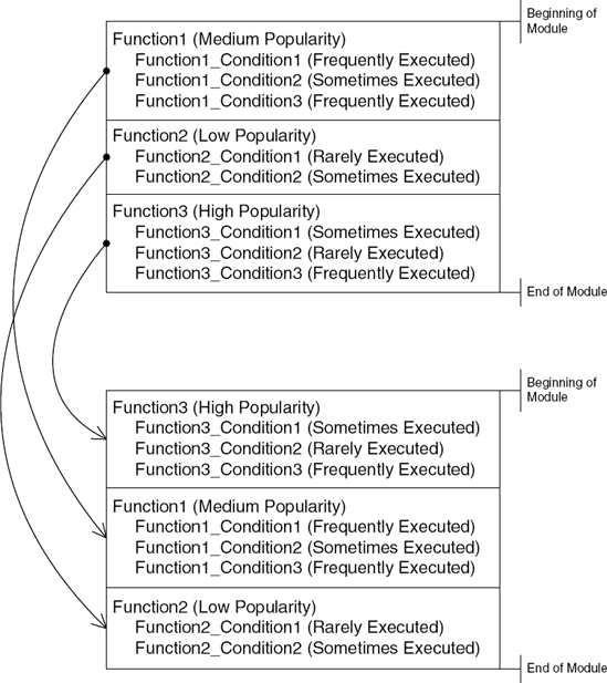
The conventional form of working-set tuning is based on a function-level reorganization. A program is launched, and the working-set tuner program observes which functions are executed most frequently. The program then reorganizes the order of functions in the binary according to that information, so that the most popular functions are moved to the beginning of the module, and the less popular functions are placed near the end. This way the operating system can keep the "popular code" area in memory and only load the rest of the module as needed (and then page it out again when it's no longer needed).
In most reversing scenarios function-level working-set tuning won't have any impact on the reversing process, except that it provides a tiny hint regarding the program: A function's address relative to the beginning of the module indicates how popular that function is. The closer a function is to the beginning of the module, the more popular it is. Functions that reside very near to the end of the module (those that have higher addresses) are very rarely executed and are probably responsible for some unusual cases such as error cases or rarely used functionality. Figure A.13 illustrates this concept.
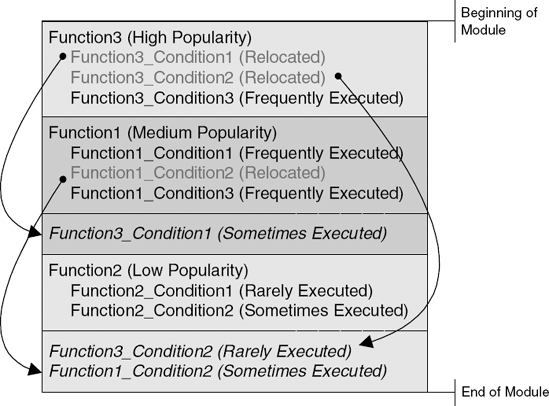
Line-level working-set tuning is a more advanced form of working-set tuning that usually requires explicit support in the compiler itself. The idea is that instead of shuffling functions based on their usage patterns, the working-set tuning process can actually shuffle conditional code sections within individual functions, so that the working set can be made even more efficient than with function-level tuning. The working-set tuner records usage statistics for every condition in the program and can actually relocate conditional code blocks to other areas in the binary module.
For reversers, line-level working-set tuning provides the benefit of knowing whether a particular condition is likely to execute during normal runtime. However, not being able to see the entire function in one piece is a major hassle. Because code blocks are moved around beyond the boundaries of the functions to which they belong, reversing sessions on such modules can exhibit some peculiarities. One important thing to pay attention to is that functions are broken up and scattered throughout the module, and that it's hard to tell when you're looking at a detached snippet of code that is a part of some unknown function at the other end of the module. The code that sits right before or after the snippet might be totally unrelated to it. One trick that sometimes works for identifying the connections between such isolated code snippets is to look for an unconditional JMP at the end of the snippet. Often this detached snippet will jump back to the main body of the function, revealing its location. In other cases the detached code chunk will simply return, and its connection to its main function body would remain unknown. Figure A.14 illustrates the effect of line-level working-set tuning on code placement.