Table of Contents for

Information Theory, Coding and Cryptography

Chapter 8

Convolution Codes

8.1  INTRODUCTION

Convolution code is an alternative to block codes, where n outputs at any given time unit depend on k inputs at that time unit as well as m previous input blocks. An (n, k, m) convolution code can be developed with k inputs, n output sequential circuit, and m input memory. The memory m must be large enough to achieve low error probability, whereas k and n are typically small integers with k < n. An important special case is when k = 1, the information sequence is not divided into blocks and can be processed continuously. This code has several practical applications in digital transmission over wire and radio channels due to its high data rate. The improved version of this scheme in the association with Viterbi algorithm led to application in deep sea and satellite communication.

8.2  TREE AND TRELLIS CODES

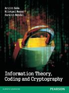
Very large block lengths have the disadvantage that the decoding procedure cannot be commenced unless the entire block of encoded data is received at the receiver. Hence, the receiving and decoding process become slow. Tree coding scheme is used to overcome this disadvantage, where uncoded information data is divided into smaller blocks or information frame of length k; information frame length may be as low as of 1 bit. These information frames are then encoded to code words frames of length n. To form a code word, the current information frame as well as the previous information frame is required. It implies that such encoding system requires memory which is accomplished by shift register in practice. The schematic diagram of encoding system for Tree codes is shown in Figure 8.1.

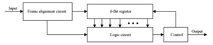
Figure 8.1 Tree Code Encoding Scheme

The information frame is stored in the shift register. Each time a new frame arrives, it is compared with the earlier frame in the logic circuit with some algorithm to form a code word and older frame is discarded, whereas new frame is loaded in the shift register. Thus for every information frame, a code word is generate for transmission.

Convolution code is one of the subclasses of Tree code. Tree code that is linear, time-invariant and having finite wordlength is called Convolution Code. On the other hand, time-invariant Tree code with finite wordlength is called Sliding Block Code. Therefore linear sliding block code is a covolution code.

Now consider a simple convolution encoder as shown in Figure 8.2 that encodes bit by bit. The input bits are loaded into registers S₁ and S₂ sequentially. The outputs of the registers are XORed with input bit and 3 bit output sequences are generated for each input bit. The outputs are tabulated in Table 8.1 for different input and register conditions. The clock rate of outgoing data is thrice as fast as the incoming data.

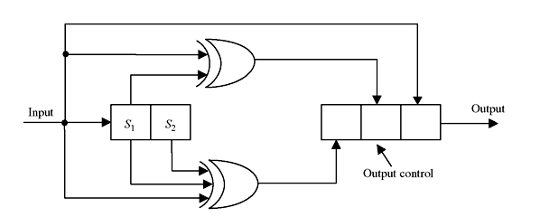
Figure 8.2 Bit by Bit Convolution Code Encoder

 

Table 8.1 Bit by Bit Convolution Encoded Output

Here, we observe that the output sequence is generate from present input and previous two input bits. The same information can be represented by state diagram as shown in Figure 8.3a. This diagram is called Trellis Diagram. The diagram can be cascaded for the stream of input bits. The cascaded form is shown in Figure 8.3b. The code may be defined as binary (3, 1, 2) convolution code.

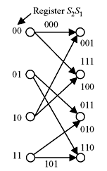
Figure 8.3a Trellis Diagram for a Single Bit

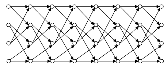
Figure 8.3b Trellis Diagram for Stream of Input Bits

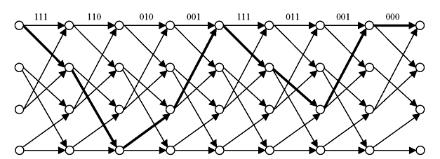
Figure 8.4a Trellis Mapping for Input Sequence 11001000

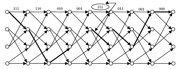
Figure 8.4b Error Location from Trellis Mapping

The name Trellis was coined because a state diagram of this technique, when drawn on paper, closely resembles the trellis lattice used in rose gardens. The speciality of this diagram is that for a sequence of input data it will follow the arrowed path. For example, let us consider the input data 11001000. Assuming initial register contents are 00, the trellis path is shown by thick lines in Figure 8.4a. Encoded bit sequence will be 111, 110, 010, 001, 111, 011, 001, and 000. If there is any break, it may be assumed that wrong data has arrived. For example, if received bit stream for the above data is 111, 110, 010, 001, 011, 011, 001 and 000, erroneous data is at the fifth sequence. There will be break at trellis mapping as shown in Figure 8.4b. It may be observed that error can be corrected by comparing the previous and succeeding data from the mapping. Therefore, at the receiver end error may be located and corrected.

8.3  ENCODING

Figure 8.5 presents schematic of an encoder for binary (2, 1, 3) code which contains linear feed-forward 3-stage shift register and modulo-2 adders (XOR). All convolution encoders can be implemented using this type of circuit. The information sequence u (u₀, u_1, u₂, …) enters the encoder bit by bit. Two sequences v⁽¹⁾ (v₀⁽¹⁾, v₁⁽¹⁾, v₂⁽¹⁾, …, v_m⁽¹⁾) and v⁽²⁾ (v₀⁽²⁾, v₁⁽²⁾, v₂⁽²⁾, …, v_m⁽²⁾) are generated which are multiplexed and the final output v (v₀, v₁, v₂, ..., v_m) is generated.

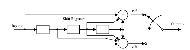
Figure 8.5 Binary (2, 1,3) Convolution Encoder

Let us consider two sequences v⁽¹⁾ and v⁽²⁾ are generated by the generator sequences (also called impulse sequences) g⁽¹⁾ (g₀⁽¹⁾, g₁⁽¹⁾, g₂⁽¹⁾, …, g_m⁽¹⁾) and g⁽²⁾ (g₀⁽²⁾, g₁⁽²⁾, g₂⁽²⁾, …, g_m⁽²⁾). The encoding equations are written as follows:

 

 

The general equation for convolution for 0 ≤ 1 ≤ i and memory m, may be written as follows:

For the encoder shown in Figure 8.5, g⁽¹⁾ = (1 0 1 1) and g⁽²⁾ = (1 1 1 1). Hence,

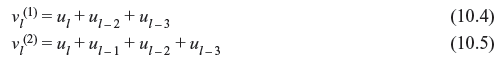
The output sequence or the code word is generated by multiplexing v⁽¹⁾ and v⁽²⁾ as follows:

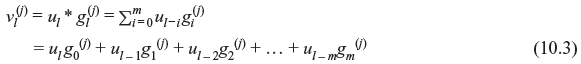
Let us consider another example of convolution encoder as shown in Figure 8.6. This is for (3, 2, 1) as this consists of m = 1 stage shift register, 2 inputs and 3 bits of output. The information sequence may be written as u = [u₀⁽¹⁾u₀⁽²⁾, u₁⁽¹⁾u₁⁽²⁾, u₂⁽¹⁾u₂⁽²⁾, …] and the output sequence or code word may be considered as v = [v₀⁽¹⁾v₀⁽²⁾ v₀⁽³⁾, v₁⁽¹⁾v₁⁽²⁾ v₁⁽³⁾, v₂⁽¹⁾v₂⁽²⁾v₂⁽³⁾, …].

It may be noted that the number of memory or shift register may not be equal in every path. Encoder memory length is defined as m = maximum of m_i, where m_i is the number of shift register at ith path.

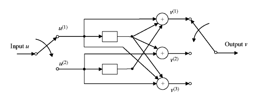
Figure 8.6 (3,2,1) Convolution Encoder

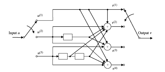
Figure 8.7 (4, 3, 2) Convolution Encoder

Figure 8.7 illustrates an example of (4, 3, 2) convolution code, where unequal numbers of shift registers exist at different input–output route. In this regard, it is useful to mention the following definitions:

1. The constraint length is defined as n_A = n(m + 1).
2. The code rate is defined as R = k/n.

Now consider for an information sequence, there are L number of blocks each consisting of k bits with m memory locations. An information sequence will be of length of kL and code word has the length n(L + m). The final nm outputs are generated after the last nonzero information block enters the encoder. The information sequence is terminated with all-zero block to allow the encoder memory clear. In comparison with the linear block codes, the block code rate of convolution code with generator matrix G is kL/n(L + m). For L >> m, L/(L + m) ≈ 1, the block code rate and convolution code rate are approximately equal. However, for small L, the effective rate of information transmission kL/n(L + m) will be reduced by a fractional amount as follows:

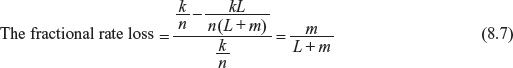
Hence, L is always is assumed to be much larger than m to keep the fractional loss small. For example, for a (2, 1, 3) convolution code of L = 5, the fractional rate loss is 3/8 = 37.5%. If L = 1000, the fractional rate loss is 3/1003 = 0.3%.

 

Example 8.1: If the message sequence is u = (10111) and generator sequences are g⁽¹⁾ = (1011) and g⁽²⁾ = (1111), find the generated code word.

Solution:

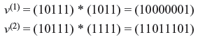
The code word is (11, 01, 00, 01, 01, 01, 00, 11)

In the other method, the generator sequences can be interlaced and expressed in matrix form as follows:

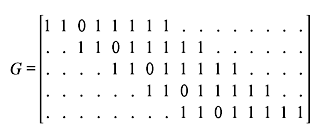
The code vector v = uG

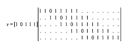
Therefore, code word is v = (11, 01, 01, 00, 01, 01, 00, 11).

 

Example 8.2: Consider a convolution code of two input sequences as u⁽¹⁾ = (101) and u⁽²⁾ = (110). If the generator sequences are g₁⁽¹⁾ = (11), g₁⁽²⁾ = (01), g₁⁽³⁾ = (11), g₂⁽¹⁾ = (01), g₂⁽²⁾ = (10), and g₂⁽³⁾ = (10). Find the code word.

 

Solution: The coding equations are

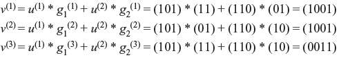
Therefore, the code word is v = (110, 000, 001, 111).

8.4  PROPERTIES

As convolution encoder is a linear system, the encoding equations can be represented by polynomials and the convolution operation may be replaced by polynomial multiplication. This means the ith input sequence u⁽ⁱ⁾(D), jth output sequence v⁽ⁱ⁾(D), and generator g can be expressed in the following forms, where 1 ≤ i ≤ k and 1 ≤ j ≤ k

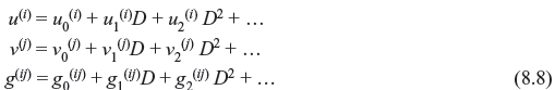
Therefore,

 

 

The indeterminate D can be interpreted as delay operator. The power of D denotes the number of time units delayed from initial bit. For a (2, 1, m) convolution code after multiplexing the output will be

 

 

In general, for an (n, k, m) convolution code, the output will be

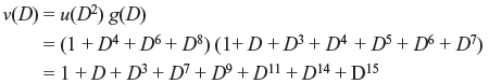
Example 8.3: For encoder shown in Figure 8.5, for (2, 1, 3) convolution code, g⁽¹⁾ = (1 0 1 1) and g⁽²⁾ = (1 1 1 1).

For u (D) = 1 + D² + D³ + D⁴, the code word is

The generator polynomials of an encoder can be determined directly from its circuit diagram and generators of complex encoder system may be represented by matrix G(D).

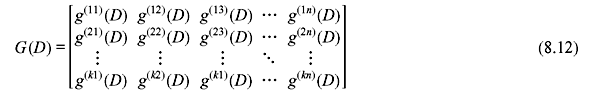
The word length of the code is max [deg g^(ij)(D)], for 1 ≤ j ≤ n.

The memory length is max [deg g^(ij)(D)], for 1 ≤ j ≤ n and 1 ≤ i ≤ k.

The constraint length is max [deg g^(ij)(D)], for 1 ≤ j ≤ n.

 

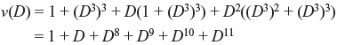
Example 8.4: For (3, 2, 1) convolution code, the generator for the encoder shown in Figure 8.6 is expressed 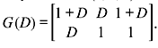Determine the code word for the inputs u⁽¹⁾ = 1 + D² and u⁽²⁾ = 1 + D.

Solution:

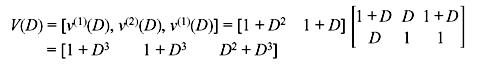
By replacing D to D³ (as n = 3) and using Eq. 8.12, we obtain the code word as

8.4.1  Structural Properties

Since the encoder for convolution code is a sequential circuit, its operation can be described by a state diagram. The state of the encoder is defined by its shift register contents. State diagram describes the transition from one state to another. Each new block of k-inputs results in transition to a new state. There are 2^k branches leaving each state. Therefore, for (n, 1, m) code, there will be only two branches leaving each state. Each transition is labelled with its input information bit and output. Figure 8.8 illustrates the state diagram for a (2, 1, 3) convolution code of encoder circuit of Figure 8.5.

Assuming that the encoder is initially at state S₀ (all-zero state), the code word for any given information sequence can be obtained from the state diagram by following the path. For example, for an information sequence of (11101) followed by nonzero bits, the code word with respect to Figure 8.8 will be (11, 10, 01, 01, 11, 10, 11, 11) and the shift registers contents return to initial state S₀.

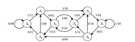
Figure 8.8 State Diagram of (2, 1, 3) Convolution Code

Similarly, a (3, 2, 1) convolution code shown in Figure 8.5 can be illustrated by the state diagram as shown in Figure 8.9. It may be noted that as k = 2, four branches are leaving from each state. There are two inputs and three outputs which are labelled in the diagram.

The state diagram can be modified to provide complete description with weight distribution function. However, the generating function approach to find the weight distribution of a convolution code is impractical. The performance may be estimated by distance properties as will be discussed in next section. An important subclass of the convolution code is the systematic code, where the first k output sequences are exactly similar to k input sequences. It will follow the condition as stated as follows:

 

 

The generator sequences satisfy

The generator matrix is given as

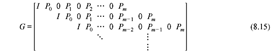
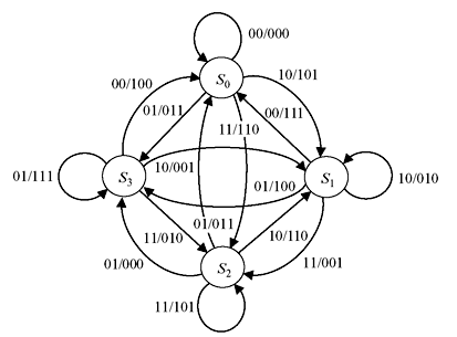
Figure 8.9 State Diagram of (3, 2, 1) Convolution Code

where I is k × k identity matrix, 0 is the k × k all-zero matrix and P_l is the k × (n − k) matrix.

The transfer function matrix will be

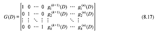
The first k output sequences equal the input sequences, and so they are called information sequences, whereas the next n − k output sequences are parity sequences. It may be noted that only k * (n − k) sequences must be specified to define a systematic code. Any code not satisfying the Eqs. (8.13) to (8.17) are called nonsystematic.

In short form Eq. (8.17) may be written as follows:

 

 

Parity-check matrix for a systematic code is

 

 

It follows that

 

 

A convolution code of transfer function matrix G(D) has a feed forward inverse G⁻¹(D) of delay l, if and only if

GCD denotes greatest common divisor. Code satisfying above equation is called noncatastrophic convolution code.

Hardware implementation is easier for systematic code as it requires no inverting circuit to recover the code word. It is to be noted that nonsystematic code can also be chosen for use in communication system, but catastrophic codes must be avoided.

 

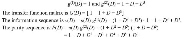
Example 8.5: Consider a (2, 1, 3) systematic code for which the generator sequences are g⁽¹⁾ = (1000) and g⁽²⁾ = (1101). Find the information sequence and parity sequence when the message sequence is u = (1011).

 

Solution:

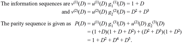
Example 8.6: Consider the (3, 2, 2) systematic code of input sequences u⁽¹⁾(D) = 1 + D and u⁽²⁾(D) = D² + D³ with transfer function matrix 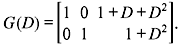Find the information sequence and parity sequence.

 

Solution:

8.4.2  Distance Properties

The performance of convolution code is governed by encoding algorithm and distance properties of the code. A good code must possess the maximum possible minimum distance. The most important distance measure for convolution codes is the minimum free distance d_free which is defined as the minimum distance between any two code words in the code.

where v′ and v′′ are code words corresponding to information sequences u′ and u′′ respectively. If u′ and u′′ are of different lengths, then zeros are added to shorter sequence to make them equal length. In other words, d_free is the minimum weight code word of any length produced by a nonzero information sequence. Also it is the minimum weight of all paths in the state diagram that diverge from and remerge with all-zero state and it is the lowest power of X in the code generating function. For example, d_free = 6 for the (2, 1, 3) code in Figure 8.8 and d_free = 3 for the (3, 2, 1) code in Figure 8.9.

Another important distance measure for convolution codes is the column distance function (CDF), which is defined by the minimum weight code word over the first i + 1 time units whose initial information block is nonzero. Let [u]_i and [v]_i be the information sequence and code word sequence, respectively, with ith truncation.

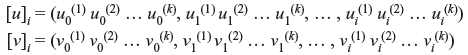
The column distance function of the order of i, d_i. is defined as

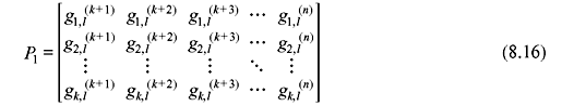
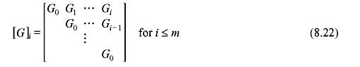
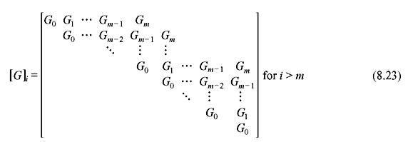
If [G]_i is the generator matrix, [v]_i = [u]_i [G]_i, where

If CDF d_i is the minimum weight code over first i + 1 time units with initial nonzero information block, it does not decrease with the increase of i. When i = m, CDF = d_m is called the minimum distance and denoted as d_min. For i → ∞ CDF reaches d_free for noncatastrophic codes; however, this may not be true for catastrophic codes.

8.5  DECODING

Although convolution encoding is a simple procedure, decoding of a convolution code is much more complex task. Several classes of algorithms exist for this purpose:

• Threshold decoding is the simplest of them, but it can be successfully applied only to the specific classes of convolution codes. It is also far from optimal.
• Sequential decoding is a class of algorithms performing much better than threshold algorithms. Their main advantage is that decoding complexity is virtually independent from the length of the particular code. Although sequential algorithms are also suboptimal, they are successfully used with very long codes, where no other algorithm can be acceptable. The main drawback of sequential decoding is unpredictable decoding latency.
• Viterbi decoding is an optimal (in a maximum-likelihood sense) algorithm for decoding of a convolution code. Its main drawback is that the decoding complexity grows exponentially with the code length. Hence, it can be utilized only for relatively short codes.

8.5.1  Threshold Decoding

Threshold decoding, also termed as majority logic decoding, is based only on the constrain length of the received blocks rather than on the received sequence to make the final decision on the received information. Its algorithm is simple and hence it is simpler in implementation comparing to other decoding techniques. However, the performance is inferior when compared to other techniques and it mainly used telephony, HF radio, where moderate amount of coding gain is required at relatively low cost.

Let us consider the systematic code with R = ½, generator sequences g⁽¹⁾ = (1 0 0 0 …) and g⁽²⁾ = (g₀⁽²⁾ g₁⁽²⁾ g₂⁽²⁾ ….). Therefore, the generator matrix i

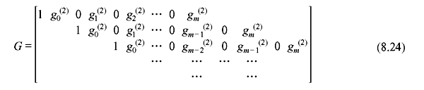
For an information sequence u, we have the equations

 

 

The transmitted code word is v = uG. If v is send over a BSC, the received sequence r may be written as follows:

The received information sequence and parity sequences, respectively, are

where e⁽¹⁾ = (e₀⁽¹⁾, e₁⁽¹⁾, e₂⁽¹⁾, …) and e⁽²⁾ = (e₀⁽²⁾, e₁⁽²⁾, e₂⁽²⁾, …) are the information error sequence and parity error sequence, respectively.

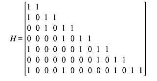
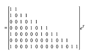
The syndrome sequence may be defined as s = (s₀, s₁, s₂, …) may be defined as          (8.29)

where H is the parity-check matrix. H is given as

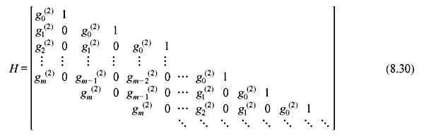
We have seen that for block codes, GH^T = 0 and v is a code word if and only if vH^T = 0. However, unlike block codes, G and H are semi-infinite as information sequences and code word are of arbitrary length for convolution codes. Since r = v + e, the syndrome can be derived as

 

 

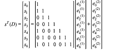
It may be noted that s depends only on the channel error and not on the code word. Hence, decoder may be designed to operate on s rather than r. Using the polynomial notation, we can write

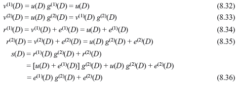
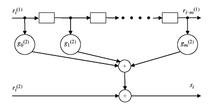
Figure 8.10 Syndrome Generation

Eq. 8.36 suggests that syndrome generation is equivalent to encoding of r⁽¹⁾ and then addition with r⁽²⁾. The implementation of it is shown in Figure 8.10.

Threshold or majority logic decoding of convolution code is based on the concept of orthogonal parity checksums. Any syndrome bit or any sum of syndrome bits which represents the sum of channel error bits is called parity checksum. If received sequence is a valid code word, the error sequence is also a code word and hence the syndrome bits as well as all parity checksum bits must be zero. If the received sequence is not a code word, the parity checksums will not be zero. An error bit e_J is said to be checked if it is checked by checksum. A set of J checksums is orthogonal on e_J, if each checksum checks e_J, but no other error bit is by more than one checksum. The value of e_J can be estimated by majority logic decoding rule.

Majority logic decoding rule correctly estimates e_J, if the error bits are checked by J orthogonal checksums containing t_ML or fewer channel errors (1’s) and estimates as e_J = 1, if and only if more than t_ML of the J checksums orthogonal e_J have value 1, where 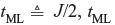is the majority logic error–correcting capability of the code. If the error bits checked by J orthogonal checksums contain t_ML or fewer channel errors, majority logic decoder correctly estimates e_J. The block diagram of decoder for self-orthogonal (n, k, m) code with majority logic decoding is given in Figure 8.11. The operation of the decoder is described as follows:

• First the constraint length of (m + 1)(n – k) syndrome bits is calculated.
• A set of J orthogonal checksums on e₀⁽¹⁾ is formed on k information error bits from the syndrome bits.
• Each set of checksums is fed into majority logic gate, where output will be ‘1’ if more than half of its inputs are ‘1’. If the output of ith threshold gate is ‘1’ [ê₀⁽ⁱ⁾ = 1], r₀⁽ⁱ⁾ is assumed to be incorrect. Correction is made by adding output of each of the threshold output to corresponding receiving bit. Threshold output is also fed back and subtracted from each of the affected syndrome bits.
• The estimated information û₀⁽ⁱ⁾ = r₀⁽ⁱ⁾ + ê₀⁽ⁱ⁾, for i = 1, 2, …., k is shifted out. The syndrome register is shifted once and receives next block of n received bits. The n – k syndrome bits are calculated and shifted into leftmost stages of n – k syndrome registers.
• The syndromes registers now contain the modified syndrome bits together with a new set of syndrome bits. The above steps are repeated to estimate the next block of information error bits. In the same way the successive blocks of information error bits are estimated.

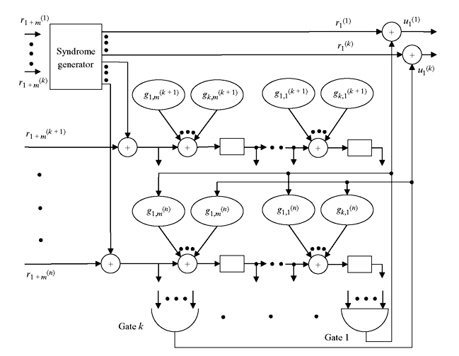
Figure 8.11 Majority Logic Decoder Scheme

Example 8.7: Consider systematic code with g⁽¹⁾(D) = 1 and g⁽²⁾(D) = 1 + D + D⁴ + D⁶. Find the majority logic error correction capability (constraint length).

 

Solution: The parity-check matrix may be developed from g⁽¹⁾(D) = 1 and g⁽²⁾(D) as

The syndrome polynomial is

The even number columns of H^T make an identity matrix. Therefore, the above equation may be rewritten by considering the odd number of columns.

It may be noted that e₀⁽¹⁾ is affected by the syndromes s₀ to s₆. The above matrix which multiplies the error sequence is called parity triangle. The parity triangle matrix is used to find out the orthogonal sets of checksums on e_J. No syndrome bit can be used for more than one orthogonal checksum as parity bit should not be checked more than once. The selection of syndrome bits is indicated by arrows as under.

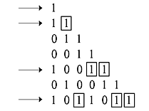
The syndrome equations may be expressed as follows:

It may be noted that no other than e₀⁽¹⁾ appears in the checksum more than once. Each checksum is single syndrome bit and so it is self-orthogonal. Since 11 different channel errors have been checked here, the effective constraint length is 11. In this case, the majority logic or threshold decoding technique can correctly estimate 2 (t_ML = 2) to 11 channel errors.

 

Example 8.8: Consider (3, 1, 4) systematic code with g⁽²⁾ = 1 + D and g⁽³⁾ = 1 + D² + D³ + D⁴. Find constraint length.

 

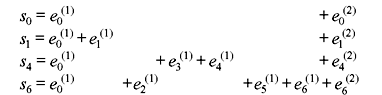
Solution: In this case, there are two syndrome sequences s₀⁽²⁾, s₁⁽²⁾, s₂⁽²⁾, s₃⁽²⁾, s₄⁽²⁾ and, s₀⁽³⁾, s₁⁽³⁾, s₂⁽³⁾, s₃⁽³⁾, s₄⁽³⁾ generated by two generator polynomials. Removing the elements of parity matrix H due to g⁽¹⁾, the syndrome equations in matrix form is as follows:

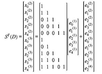
Now two parity triangles are used to investigate the checksums. Useful syndromes are indicated by arrows. The checksums s₀⁽²⁾, s₀⁽³⁾, s₁⁽²⁾, s₂⁽³⁾, s₂⁽²⁾ + s₄⁽³⁾ and s₁⁽³⁾ + s₃⁽³⁾ form six orthogonal sets of e₀⁽¹⁾.

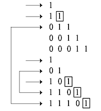
Since 13 different channel errors have been checked here, the effective constraint length is 13. It can estimate 3 (t_ML = 3) to 13 errors correctly.

8.5.2  Sequential Decoding

The decoding effort of sequential decoding is independent of encoder memory k and hence large constraint lengths can be used. Sequential decoding can achieve a desired bit error probability when a sufficiently large constraint length is taken for the convolution code. We shall see that decoding effort of it is also adaptable to the noise level. Its main disadvantage is that noisy frame requires large amount of computation and decoding time occasionally exceed some upper limit, causing information to be lost or erased.

The 2^KL code words of length N = n(L + m) for an (n, k, m) code and an information sequence of length KL as paths may be conveniently represented by code-tree containing L + m + 1 time units or levels. The code-tree is an expanded version of trellis diagram where every path is distinct and totally different from every other path. The code-tree for (3, 1, 2) code with G(D) = [1 + D, 1 + D², 1 + D + D²] is given at Figure 8.12 for information sequence length L = 5. The number of tree levels is L + m + 1 = 5 + 2 + 1 = 8 which is labelled as 0 to 7. The leftmost node in the tree is called origin node representing the starting state S₀ of the encoder. There are 2^k branches leaving every node in the first L levels (i.e., five levels in this example) termed as dividing part of the tree. The upper branch of each node represents input u_i = 1, while the lower branch represents u_i = 0. After L levels, there is only one branch leaving each node. This represents u_i = 0 for i = L, L + 1, …, L + M − 1 corresponding to the encoder’s return to all-zero state S₀. This part is called tail of the tree and the rightmost nodes are termed as terminal nodes.

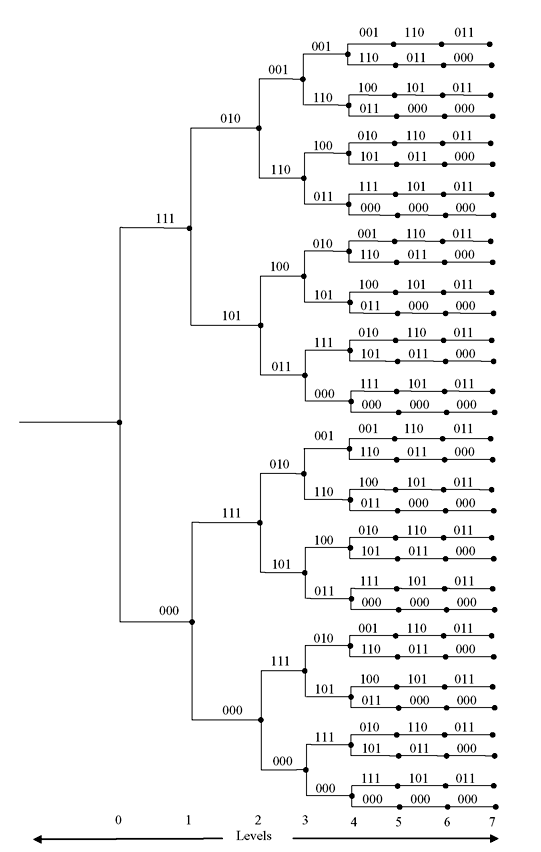
Figure 8.12 Code Tree for (3, 1, 2) Code of Sequence Length L = 5

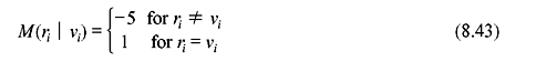
The purpose of sequential decoding algorithm is to find the maximum likelihood path by searching through nodes of the code tree in an efficient way. Involvement of any particular path at the maximum likelihood path depends on its metric value associated with that path. The metric is a measure of the closeness of a path to the received sequence. The bit metric is given as follows:

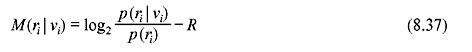
where P(r_i | v_i) is the channel transition probability, P(r_i) is the channel output symbol probability, and R is the code rate. The partial path metric for the first l branch is given as follows:

where M(r_j | v_j) is the branch metric for jth branch. Combining Eqs. (8.37) and (8.38), we obtain

For a symmetric channel with binary input and Q-ary output,

Then Eq. (8.39) reduces to

In general, for a BSC with transition probability p, the bit metrics are

A. Stack Algorithm  In the stack algorithm, also called as ZJ algorithm, the stack or ordered list of previously examined paths of different lengths is kept in storage. Each stack entry contains a path along with its metric. Path of largest metric is placed on top and others are listed in decreasing order of metric. Each decoding step consists of extending the top path in the stack by computing the branch metrics of its 2^k succeeding branches and then adding these to the metric of top path to form 2^k new paths, which are called successors of top path. The top path is now deleted, its 2^k successors are inserted and stack is rearranged. Algorithm terminates when the top path in the stack is at the end of the tree. At this point, the top path is the decoded path. The procedure can be described by a flow chart as shown in Figure 8.13. The size of stack is roughly equal to the number of decoding steps when algorithm terminates.

The number of stack computation for stack algorithm is higher than the Viterbi algorithm. However, since very noisy received sequence does not occur very often, the average number of computation by a sequential decoder sometimes less than that of Viterbi algorithm. There exists some disadvantages in the implementation of stack algorithm. First, since the decoder traces somewhat back and forth through code tree, the decoder must require input buffer to store the incoming sequences to keep them at waiting. The speed factor of the decoder, ratio of speed of computation to the rate of incoming data, plays an important role. Second, the size of stack must be finite, otherwise there are always some probabilities that the stack will fill up before decoding is complete. The most common way of handling this problem is to push out or discard the path at the bottom of the stack on the next decoding step. Third, rearrangement of stack may be time-consuming if number of stack is high.

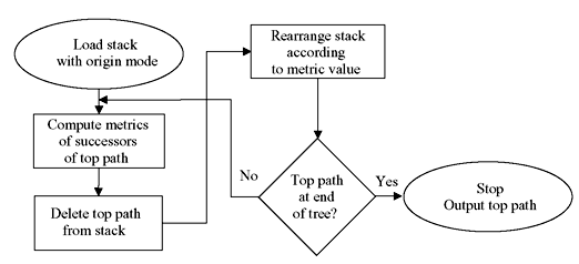
Figure 8.13 Flow Chart for Stack Algorithm

B. Fano Algorithm  Fano algorithm approach of sequential decoding requires no storage with the sacrifice of speed compared to stack algorithm. In Fano algorithm, the decoder examines a sequence of nodes in the tree starting from the origin node and ending at terminal node. The decoder never jumps from node to node as in stack algorithm, but moves to adjacent node. The metric at each node is calculated at that instant by addition or subtraction of metric of connecting branch. Thus need of storing the metrics is eliminated. However, some nodes are revisited and metrics are recalculated. The decoder will move forward as long as the metric value along the path examined continues to increase. When the metric value dips below a certain threshold, the decoder selects another path to examine. If no path is observed below threshold, the threshold value is lower and examination procedure is started again. The decoder eventually reaches the end of the tree, where the algorithm terminates. This operation is described by a flow chart as shown in Figure 8.14. The decoder starts at origin with threshold T = 0 and metric value M = 0. It looks forward to the best of the 2^k succeeding nodes, i.e., the one with largest metric. If M_F is the metric of forward node being checked and if M_F > T, decoder moves in this node. Threshold modification or threshold tightening is performed if the node is visited first time. Threshold T is increased by largest possible multiple of a threshold increment Δ so that the new threshold does not exceed current metric. Threshold tightening is not required if the node is visited previously.

If M_F < T, the decoder looks backward to the proceeding node. If M_B is the metric of backward node being examined, and if M_B < T, then T is decreased by Δ and looks forward to the best node. If in this checking process M_B > T and this backward move is from worst of the 2^k succeeding nodes, the decoder again looks back to the preceeding node, else the decoder looks forward to the next best of 2^k nodes. If the decoder ever looks backward from origin node, it is assumed to be metric value of ∞.

The number of computations in Fano algorithm depends on the selection of threshold increment Δ. If it is too small, the number of computations is large. It may be noted that the metrics are scaled by a positive constant so that they can be closely approximated as integers for easier implementation. For example, for R = 1/3 and p = 0.10, from Eq. (8.37) we get

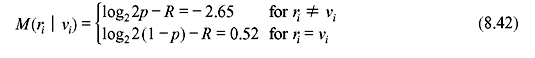
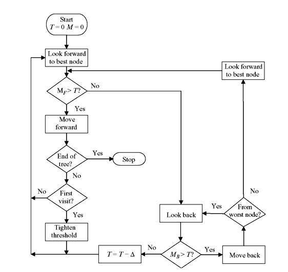
Figure 8.14 Flow Chart for Fano Algorithm

The above equation may be normalized with the scaling factor of 1/0.52 and approximated to integers as follows:

C. Performance  Let the jth incorrect subset of the code tree be the set of all nodes branching from jth node on correct path, 0 ≤ j ≤ L − 1, where L is the length of the information sequence in branches. If C_j represents the number of computations performed in the incorrect subset, the average probability distribution of the ensemble of all convolution codes satisfies

 

 

where A is a constant for particular version of sequential decoding. For channel capacity of C, ρ is related to code rate R and Gallager function E₀(ρ) as follows:

For any binary input discrete memoryless channel (DMC), E₀(ρ) is given as follows:

where p is the channel transition probability. If ρ ≤ 1, the mean number of computations per decoded branch is unbounded. Therefore, R is bounded to R₀, when ρ = 1. R₀ is called computational cutoff rate of the channel. Hence, R must be less than R₀, for finite number of computation. The probability distribution of Eq. (8.44) may also be used to calculate the probability of buffer overflow or the erasure probability. When B is the capacity of input buffer i branches (nB bits), μ is the speed factor of decoder and L is information length, the erasure probability is given as follows:

 

 

It may be noted that erasure probability does not depend on code constraint length.

For high rates (R > R₀), the undetected error probability in sequential decoding is same as in maximum likelihood decoding and is therefore optimum. The average error probability in sequential decoding is suboptimum at low rates when R < R₀ and it can be compensated using higher values of constraint length K, as the computational behaviour of sequential decoding is independent of K. The overall performance can be optimized by obtaining trade-offs among three governing factors of performance characteristics—average computational cutoff, erasure probability, and undetected error probability.

8.5.3  Viterbi Decoding

Viterbi decoding algorithm is the most optimum to decode convolution code to produce the maximum likelihood estimate of the transmitted sequence over a band limited channel with intersymbol interference. It may be observed that in a convolution code, the channel memory that produces the intersymbol interference is analogous to the encoder memory. The Viterbi algorithm is a dynamic programming algorithm for finding the most likely sequence of hidden states—called the Viterbi path—that results in a sequence of observed events. The forward algorithm is a closely related algorithm for computing the probability of a sequence of observed events. These algorithms belong to the realm of probability theory. The algorithm makes a number of assumptions:

• First, both the observed events and hidden events must be in a sequence. The sequence is often temporal, i.e., in time order of occurrence.
• Second, these two sequences need to be aligned: An instance of an observed event needs to correspond to exactly one instance of a hidden event.
• Third, computing the most likely hidden sequence (which leads to a particular state) up to a certain point t must depend only on the observed event at point t, and the most likely sequence which leads to that state at point t − 1.

The above-mentioned assumptions can be elaborated as follows. The Viterbi algorithm operates on a state machine assumption. This means, at any time the system being modelled is in one of a finite number of states. While multiple sequences of states (paths) can lead to a given state, at least one of them is a most likely path to that state, called the survivor path. This is a fundamental assumption of the algorithm because the algorithm will examine all possible paths leading to a state and only keep the one most likely. This way, it is sufficient that the algorithm keeps a track of only one path per state and not necessary to have a track of all possible paths.

A second key assumption is that a transition from a previous state to a new state is marked by an incremental metric, usually a number. This transition is computed from the event. The third key assumption is that the events are cumulative over a path in some sense, usually additive. So the crux of the algorithm is to keep a number for each state. When an event occurs, the algorithm examines moving forward to a new set of states by combining the metric of a possible previous state with the incremental metric of the transition due to the event and chooses the best. The incremental metric associated with an event depends on the transition possibility from the old state to the new state. For example in data communications, it may be possible to transmit only half the symbols from an odd numbered state and the other half from an even numbered state. Additionally, in many cases, the state transition graph is not fully connected. After computing the combinations of incremental metric and state metric, only the best survives and all other paths are discarded.

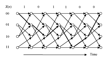
Figure 8.15 Trellis Diagram

The trellis provides a good framework for understanding decoding and the time evolution of the state machine. Suppose we have the entire trellis in front of us for a code, and now receive a sequence of digitized bits. If there are no errors (i.e., the noise is low), then there will be some path through the states of the trellis that would exactly match up with the received sequence as shown in Figure 8.15.

That path (specifically, the concatenation of the encoding of each state along the path) corresponds to the transmitted parity bits. From there, getting to the original message is easy because the top arc emanating from each node in the trellis corresponds to a ‘0’ bit and the bottom arrow corresponds to a ‘1’ bit. When there are errors, finding the most likely transmitted message sequence is appealing because it minimizes the BER. If the errors introduced by going from one state to the next are captured, then accumulation of those errors along a path comes up with an estimate of the total number of errors along the path. Then, the path with the smallest such accumulation of errors is the desired path, and the transmitted message sequence can be easily determined by the concatenation of states explained above. Viterbi algorithm provides a way to navigate the trellis without actually materializing the entire trellis (i.e., without enumerating all possible paths through it and then finding the one with smallest accumulated error) and hence provides optimization with dynamic programming.

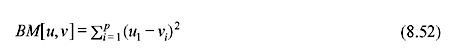
A. Viterbi Decoder   The decoding algorithm uses two metrics: The branch metric (BM) and the path metric (PM). The branch metric is a measure of the ‘distance’ between the transmitted parity bits and the received ones, and is defined for each arc in the trellis. In hard decision decoding, where a sequence of digitized parity bits are transmitted, the branch metric is the Hamming distance between the expected parity bits and the received ones.

An example is shown in Figure 8.16, where the received bits are 00. For each state transition, the number on the arc shows the branch metric for that transition. Two of the branch metrics are 0, corresponding to the only states and transitions where the corresponding Hamming distance is 0. The other nonzero branch metrics correspond to cases when there are bit errors. The path metric is a value associated with a state in the trellis (i.e., a value associated with each node). For hard decision decoding, it corresponds to the Hamming distance over the most likely path from the initial state to the current state in the trellis. Most likely path is referred to the path with smallest Hamming distance between the initial state and the current state, measured over all possible paths between the two states. The path with the smallest Hamming distance minimizes the total number of bit errors, and is most likely when the BER is low.

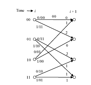
Figure 8.16 Branch Metric and Path Metric

B. Computation of Path Metric  The key insight in the Viterbi algorithm is that the receiver can compute the path metric for a (state, time) pair incrementally using the path metrics of previously computed states and the branch metrics. Suppose the receiver has computed the path metric PM[s, i] for each state s (of which there are 2^{k − 1} states, where k is the constraint length) at time step i. The value of PM[s, i] is the total number of bit errors detected when comparing the received parity bits to the most likely transmitted message, considering all messages that could have been sent by the transmitter until time step i (starting from state ‘00’).

Among all the possible states at time step i, the most likely state is the one with the smallest path metric. If there is more than one such state, they are all equally good possibilities. Now, to determine the path metric at time step i + 1, PM[s, i + 1], for each state s, it is first to be observed that if the transmitter is at state s at time step i + 1, then it must have been in only one of two possible states at time step i. These two predecessor states, labelled α and β, are always the same for a given state. In fact, they depend only on the constraint length of the code and not on the parity functions. Figure 8.16 shows the predecessor states for each state (the other end of each arrow). For instance, for state 00, α = 00 and β = 01; for state 01, α = 10 and β = 11. Any message sequence that leaves the transmitter in state s at time i + 1 must have left the transmitter in state α or state β at time i. For example, in Figure 8.16, to arrive at state ‘01’ at time i + 1, one of the following two properties must hold:

1. If the transmitter is in state ‘10’ at time i and the ith message bit is a 0, then the transmitter sents ‘11’ as the parity bits and there are two bit errors, because we receive the bits 00. Then, the path metric of the new state, PM[‘01’, i + 1] = PM[‘10’, i] + 2, because the new state is ‘01’ and the corresponding path metric is larger by 2 because there are two errors.
2. The other (mutually exclusive) possibility is that if the transmitter is in state ‘11’ at time i and the ith message bit is a 0, then the transmitter sents 01 as the parity bits and there is one bit error, because we receive the bits 00. Then, the path metric of the new state, PM[‘01’, i + 1] = PM[‘11’, i] + 1. Formalizing the above intuition, where α and β are the two predecessor states, we can easily say that

In general, for a Q-ary system, the mathematical representation can be given as below. Let us consider that an information sequence u = (u₀, u₁, …, u_L _ ₁) of length kL is encoded into a code word v = (v₀, v₁, …, v_{L + m − 1}) of length N = n(L + m) which is received as the Q-ary sequence r = (r₀, r₁, …, r_{L – 1}) over a DMC. A decoder must produce an estimate of the code word which maximizes the log-likelihood function log P(r | v). P(r | v) is the channel transition probability.

If the term P(r_i | v_i) is denoted as M(r_i | v_i), which is called branch metric, and hence the path metric M(r | v) may be written as follows:

The above equation holds good to find a path v that maximizes M(r | v).

In the decoding algorithm, it is important to remember which arc corresponds to the minimum, because it is required to traverse this path from the final state to the initial one, keeping track of the arcs used, and then finally reverse the order of the bits to produce the most likely message.

C. Finding the Most Likely Path  Initially, state ‘00’ has a cost of 0 and the other 2^k−1 − 1 states have a cost of ∞. The main loop of the algorithm consists of two main steps: Calculating the branch metric for the next set of parity bits and computing the path metric for the next column. The path metric computation may be thought of as an add–compare–select procedure:

1. Add the branch metric to the path metric for the old state.
2. Compare the sums for paths arriving at the new state (there are only two such paths to compare at each new state because there are only two incoming arcs from the previous column).
3. Select the path with the smallest value, breaking ties arbitrarily. This path corresponds to the one with fewest errors.

Figure 8.17 shows the algorithm in action from one time step to the next. This example shows a received bit sequence of 11 10 11 00 01 10 and how the receiver processes it. It may be noted that the paths of minimum path metric have been chosen and two likely paths or survivor paths are shown with thick lines. It may also be observed that all four states at fourth stage have the same path metric. At this stage, any of these four states and the paths leading up to them are most likely transmitted bit sequences (they all have a Hamming distance of 2). After final stage, the path following least values of path metric is chosen as shown at Figure 8.18. The corresponding message bits are 101100.

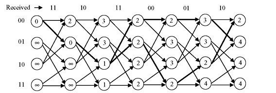
Figure 8.17 Trellis Diagram for Received Bit Sequences 11 10 11 00 01 10

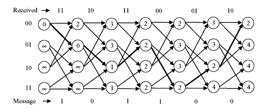
Figure 8.18 Selection of Least Values of Path Metric

A survivor path is one that has a chance of being the most likely path; there are many other paths that can be pruned away because there is no way in which they can be most likely. The reason why the Viterbi decoder is practical is that the number of survivor paths is much, much smaller than the total number of paths in the trellis. Another important point about the Viterbi decoder is that future knowledge will help it break any ties, and in fact may even cause paths that were considered ‘most likely’ at a certain time step to change.

Example 8.9: The received code word of binary (3, 1, 2) convolution code follows the trellis diagram as (000, 111, 110, 010, 100, 011, 001, 000) as survival path. Assuming the trellis diagram (Figure 8.3b), find the information code after decoding.

The survival path has been shown as thick lines in the trellis diagram (Figure 8.19). The decoded information vector is v = (01101000).

Viterbi algorithm is also applicable to soft decision decoding where decoding deals with the voltage signals. It does not digitize the incoming samples prior to decoding. Rather, it uses a continuous function of the analogue sample as the input to the decoder. Soft decision metric is the square of the difference between the received voltage and the expected one. If the convolution code produces p parity bits, and the p corresponding analogue samples are v = (v₁, v₂, …,v_p), one can construct a soft decision branch metric as follows:

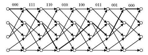
Figure 8.19 Survival Path of Example 8.9

where u = u₁, u₂, …, u_p are the expected p parity bits (each a 0 or 1). With soft decision decoding, the decoding algorithm is identical to the one previously described for hard decision decoding, except that the branch metric is no longer an integer Hamming distance but a positive real number (if the voltages are all between 0 and 1, then the branch metric is between 0 and 1 as well).

D. Performance Issues  There are three important performance parameters for convolution coding and decoding: (1) state and space requirement of encoder, (2) time required by the decoder, and (3) amount of reduction in the bit error rate and comparison with other codes. The amount of space requirement is linear in K, the constraint length, and the encoder is much easier to implement than the Viterbi decoder. The decoding time depends mainly on K. We need to process 2^K transitions each bit time, so the time complexity is exponential in K. Moreover, as described, we can decode the first bits of the message only at the very end. A little thought will show that although a little future knowledge is useful, it is unlikely that what happens at bit time 1000 will change our decoding decision for bit 1, if the constraint length is, say, 6. In fact, in practice, the decoder starts to decode bits once it has reached a time step that is a small multiple of the constraint length; experimental data suggests that 5K message bit times (or thereabouts) are reasonable decoding window, regardless of how long the parity bit stream corresponding to the message it.

The reduction in error probability and comparisons with other codes is a more involved and detailed issue. The answer depends on the constraint length (generally speaking, larger K has better error correction), the number of generators (larger this number, the lower the rate, and the better the error correction), and the amount of noise.

To analyze the performance bound, let us consider that a first event error occurred at time unit j which is in the incorrect path. The incorrect path emerges from correct path and remerges at j time unit. There may be a number of incorrect paths. The number of code word is A_d, and the first error probability is P_d, for the incorrect path weight of d. Then the first error probability at j time unit, P_j(E, j) is bounded by the sum of all error probabilities, such that

Since the bound is independent of j, it holds for all time units and hence the first error probability at any time, P_j(E) is bounded by

If the BSC transition probability is p, mathematical derivation shows that

For an arbitrary convolution code with generating function, Eq. 8.51 may be written as follows:

 

Since the event error probability is equivalent to first error probability and independent of j at any time unit, it can be derived as follows:

For small p, the above equation is approximated as follows:

The event error probability can be modified to provide bit error probability, P_b(E), i.e., the expected number of information bit decoding errors per decoded information bit. Each event error causes a number of information bit errors equal to the number of nonzero information bits on the incorrect path. If the number of information bit per unit time is k, and total number of nonzero information bits on all weight d path is B_d, the bit error probability is bounded as follows:

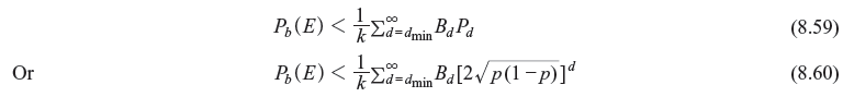
For small p, bound of bit error probability is

If E is the energy transmitted and N₀ is the one-sided noise spectral density, we have the maximum transition probability

If free distance for a convolution code is d_free, we may rewrite the Eq. (8.57) as follows:

When p is small, i.e., E/N₀ is large, energy per information bit is, and transmitted symbols per information bit is 1/R, we may write

Without coding, i.e., R = 1, the transition probability p is equivalent to P_b(E) and hence

Comparing Eqs. (8.64) and (8.65), we may calculate the asymptotic gain, γ = Rd_free/2. γ in decibel is calculated as follows:

For large E_b/N₀ at AWGN channel, the bound of P_b(E) is approximated as follows:

As the bit error probability at AWGN is approximately twice of BSC channel. At same bit error probability, AWSN channel has 3 dB power advantages over BSC channel. This illustrates the benefit of unquantized decoder where soft decision decoding may be done. However, the decoder complexity increases. It is observed that for quantization level Q of 8, performance within ¼ dB of optimum may be achieved as compared to analogue decoding. Random coding analysis has also shown the power advantage at soft decision over hard decision by 2 dB for small E_b/N₀. Over the entire range of E_b/N₀ the decibel loss associated for hard decision is 2 to 3 dB.

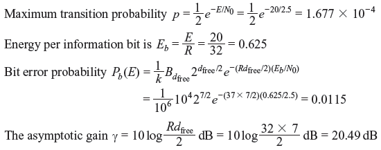
Example 8.10: An AWSN channel has the capacity of transmission of 10⁶ information bits per second and noise power of 2.5 W. Information is transmitted over this channel with signal power of 20 W, d_free of 7, total number of nonzero information bits of 10⁴. Every symbol is represented by 32 bits. What is the bit error probability of this channel with coding? What is the asymptotic gain?

Solution:

8.6  CONSTRUCTION

The performance bound analysis suggests that to construct good convolution codes, free distance d_free is required to be as large as possible. Other governing factors are number of code words A_dfree with weight d_free, and the total information sequence of all weight d_free code words, B_dfree . Under all circumstances the catastrophic codes should be avoided.

Most code construction for convolution codes are being done by computer search. It has been proved difficult to find the algebraic structures for convolution codes, which assure good distance properties, similar to the BCH construction for block codes. As most computer search techniques are time-consuming, construction of long convolution code is avoided and convolution code of relatively short constraint lengths is used. Computer construction techniques for noncatastrophic codes with maximum free distance has delivered quite a few number of codes for various coderates R. Basic rules of construction of good convolution codes are stated as under.

Let us consider g(x) is the generator polynomial of any (n, k) cyclic code of odd length n with minimum distance d_g and h(x) = (Xⁿ − 1)/g(x) is the generator polynomial of (n, n − k) dual code with minimum distance d_h. For any positive integer l, the rate R = ½l convolution code with composite generator polynomial g(D) is noncatastrophic and has d_free ≥ min (d_g, 2d_h). Since the lower bound on d_free is independent of l, the best code will be obtained when l = 1, i.e., R = ½. The cyclic codes should be selected so that d_g = 2d_h, suggesting that cyclic codes within the range 1/3 ≤ R ≤ ½ may be used for best performance.

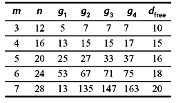
For any positive integer l, convolution code of the rate R = 1/4l with composite generator polynomial g(D²) + Dh(D²) is noncatastrophic and has the characteristics of d_free ≥ min (d_g + d_h, 3d_g, 3d_h). Since the lower bound on d_free is independent of l, the best code will be obtained when l = 1, i.e., R = ¼. The cyclic codes should be selected so that d_g = d_h, suggesting that cyclic codes with R = ¼ may be used for best performance. Some of the good convolution codes are given in Tables 8.2, 8.3, and 8.4.

 

 

Table 8.2 R = 1/2

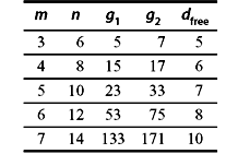
Table 8.3 R = 1/3

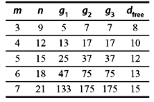
Table 8.4 R = 1/4

Absence of good, long cyclic codes and dependence of the bound on the minimum distance of the dual cyclic codes are the factors that prevent construction of long convolution codes. In certain cases as observed by Justesen, construction yields the bound d_free ≥ d_g, but a rather complicated condition on the roots of g(x) is involved and in binary case, only odd values of n can be used to construct convolution codes.

8.7  IMPLEMENTATION AND MODIFICATION

The basic working of Viterbi algorithm has been discussed so far. But there involves several other factors in practical implementation of the algorithm.

• Code Performance—Performance of codes has been discussed in the earlier section. The bit error probability P_b(E) with respect to E_b/N₀ is affected by encoder memory k, quantization levels Q, and code rate. E_b/N₀ decreases with the increase in encoder memory as well as quantization levels. Reduction in coderate increases the performance. Therefore, one has to consider all these aspects while considering a convolution code.
• Decoder Synchronization—In practice, decoder does not always commence its decoding process at the first branch transmitted after the encoder is set to all-zero state. It may begin with the encoder in an unknown state and decoding may start in the middle of trellis. Therefore, when memory truncation is used, the initial decision based on the survivor with the best metric is unreliable causing initial decoding errors. However, random coding arguments show that after about 5m branches of decoding the effect of initial lack of branch synchronization is negligible and can be discarded.

  Bit or symbol synchronization is also required by the decoder. An initial assumption is made by the decoder. If this assumption is incorrect, the survivor metrics remain relatively close together. This produces a stretch of data that seems contaminated by noisy channel. Such condition of long enough span is the indication of incorrect bit or symbol synchronization, as long stretches of noise is very unlikely. The symbol synchronization assumption is made reset until correct synchronization is achieved. It may be noted that at most n attempts are needed to acquire symbol synchronization.

• Decoder Memory—It may be observed that there are 2^k states in the state diagram of the encoder and hence the decoder must provide 2^k words of storage for the survivors. Each word must be capable of storing survivor paths along with its metric. As storage requirements increase exponentially with k, it is not practically feasible to use the codes of large values of k. The practical limit of k is considered to be about 8 for implementation of Viterbi algorithm. Thus available free distance also becomes limited. The achievable error probability cannot be made arbitrarily small for Viterbi algorithm accordingly the performance bounds as discussed above. In most cases of soft decision decoding, the practical limit of coding gain and error probability are around 7 dB and 10⁻⁵, respectively. The exact error probability depends on the code, its rate, free distance, signal-to-noise ratio (SNR) of the channel and the demodulator output quantization as well as the other factors.
• Path Memory—It has been noted that an encoder memory of order m, an information sequence of length kL and factor m(L + m) govern the fractional loss in effective rate of transmission compared to the code rate R. Since, energy per information bit is inversely proportional to the rate, E_b/N₀ is required to be larger for lower effective rate to achieve a desired performance. Therfore, L is desired to be large as possible so that the effective rate is nearly R. Thus, the need of inserting m blocks of 0’s into input stream is reduced after every blocks of information bits.

For very large L, it is practically impossible to implement as each of the 2^k words as storage must be capable of storing kL bits path with its metric. Some compromises are made by truncating the path memory of the decoder by storing only the most recent τ blocks of the information bits for each survivor, where τ = L. Each τ blocks of the received sequence is processed by the decoder replacing the previous block. Decoder must decide at the previous block since they can no longer be stored. There are several strategies for making the decision:

1. An arbritary survivor is selected and the first k bits on this path are chosen for decoded bits.
2. One of the survivor is selected which appears most often in the 2^k survivors from among the 2^k possible information blocks.
3. The survivor with the best metric may be selected and the first k bits on this path are considered as the decoded bits.

After the first decoding decision, next decoding decisions are made in the similar way for each new received block processed. Therefore, the decoding decision always lags the progress of the decoder an amount equal to τ blocks. The decoder in this case is no longer to be of maximum likelihood but results are almost as good if τ is not too small. It has been observed that if τ is in the order of five times the encoder memory or more, the probability of all survivors stem from the same information block τ time units back approaches to 1 and hence the decoding decision is unambiguous. If τ is large enough almost all decoding decisions will be equivalent to maximum likelihood and final decoded sequence is close to maximum likelihood path. It may be noted that the final decoded data may not be error-free, as the final path may not correspond to actual trellis path.

In truncated decoder memory, there are two ways that error can be introduced. Any branch decision at time unit j is made by selecting survivor at time unit j + τ with best metric becomes erroneous, if error is introduced at time unit j. As it is assumed the maximum likelihood path is best survivor at j + τ time unit, the truncated decoder will contain same error. Another source of error is when an incorrect path that is unmerged with correct path from time unit j through time unit j + τ, is the best survivor at time unit j + τ. Decoder error is observed at time unit j, though incorrect path is eliminated when it later remerges with correct path.

The limitation on practical application of Viterbi algorithm is the storage of 2^k words complexities of decoding process. Also 2^k comparisons must be performed in each time unit, which limits the speed of the processing. These leads to little modification in Viterbi algorithm. First, k is selected as 8 or less so that exponential dependence on k is limited. Second, the speed limitation can be improved by employing parallel decoding. Employment of 2^k identical parallel processing can perform all 2^k comparisons in single time unit instead rather than having one processor to perform all 2^k comparisons in sequence. Therefore, parallel decoding implies speed advantage of the factor of 2^k, but hardware requirement increases substantially.

One approach to reduce the complexities of Viterbi algorithm is to reduce the number of states in the decoder which is termed as reduced code. The basic idea is to design the decoder assuming less amount of encoder memory. This eventually reduces the effective free distance of the code. Another approach is to try to identify subclasses of codes that allow a simplified decoding structure. But this approach does not yield the optimum free distance codes.

8.8  APPLICATIONS

Convolution codes have been extensively used in practical error control applications on a variety of communication channels. Convolution encoding with Viterbi decoding is a forward error correction (FEC) technique that is particularly suited to a channel in which the transmitted signal is corrupted mainly by additive white gaussian noise (AWGN).

The Viterbi algorithm was conceived by Andrew Viterbi in 1967 as a decoding algorithm for convolution codes over noisy digital communication links. The algorithm has found universal application in decoding the convolution codes used in both CDMA and GSM digital cellular, dial-up modems, satellite, deep space communications, and 802.11 wireless LANs. It is commonly used even now in speech recognition, keyword spotting, computational linguistics, and bioinformatics. For example, in speech-to-text (speech recognition), the acoustic signal is treated as the observed sequence of events, and a string of text is considered to be the ‘hidden cause’ of the acoustic signal. The Viterbi algorithm finds the most likely string of text given the acoustic signal.

The Linkabit Corporation has designed and developed convolution encoder/Viterbi decoder codecs for a wide variety of applications. The Defense Satellite Communication System has employed soft decision hardware of the above, capable of operation at 10 Mb/s. NASA’s CTS satellite system uses multiple-rate Viterbi coding system. High-speed decoder of the speed of 160 Mb/s has been employed in Tracking and Data Relay Satellite System (TDRSS) by NASA. Its concatenation schemes are found to have many applications at space and satellite communication.

Sequential decoding is also used in many of NASA application for deep space mission. One of these, a 50 Mb/s hard decision Fano decoder remains the fastest sequential decoder is used on a NASA space station-to-ground telemetry link. Another flexible Fano decoder is capable of handling memory orders from 7 to 47, systematic and non-systematic codes, variable frame lengths, hard or soft decisions with 3 × 10⁶ computations per second, and is used in a variety of NASA applications including TELOPS programme, the International Ultraviolet Explorer (IUE) telemetry system, and International SUN-Earth Explorer (ISEE) programme. Hard decision Fano decoder hardware has also been deployed for US Army Satellite Communication Agency’s TACSAT channel and NASA’s digital television set. Extremely low frequency (ELF) band application of Fano decoder has been deployed in US Navy’s project to facilitate the communication with submarines around the world where frequency of around 76 Hz and data rate as low as 0.03 bps has been used.

Majority logic decoder for self-orthogonal code is used in PCM/FDMA system (SPADE) with transmitting data rate of 40.8 kb/s over regular voice channels of INTELSAT system. This has the applications at PSK, FSK systems, terrestrial telephone lines, and airborne satellite communication.

8.9  TURBO CODING AND DECODING

Simple Viterbi-decoded convolution codes are now giving way to turbo codes, a new class of iterated short convolution codes that closely approach the theoretical limits imposed by Shannon’s theorem with much less decoding complexity than the Viterbi algorithm on the long convolution codes that would be required for the same performance. Concatenation with an outer algebraic code [e.g., Reed–Solomon (R-S)] addresses the issue of error floors inherent to turbo code designs.

In information theory, turbo codes (originally in French Turbocodes) are a class of high-performance FEC codes developed in 1993, which were the first practical codes to closely approach the channel capacity, a theoretical maximum for the code rate at which reliable communication is still possible given a specific noise level. Turbo codes are finding the use in (deep space) satellite communications and other applications where designers seek to achieve reliable information transfer over bandwidth- or latency-constrained communication links in the presence of data-corrupting noise. Turbo codes are nowadays competing with LDPC codes, which provide similar performance.

Turbo codes are a quasi-mix between block code and convolution code. Like block codes, turbo codes require the presence of whole block before encoding can begin. However, the computation of parity bits is performed with the use of shift registers like convolution codes. Turbo codes typically use at least two convolution component encoders separated by interleaver. This is process is called concatenation. Three different arrangements are used for turbo codes which are as follows:

1. Parallel Concatenation Convolution Codes (PCCC)
2. Serial Concatenation Convolution Codes (SCCC)
3. Hybrid Concatenation Convolution Codes (HCCC)

Typically turbo codes are arranged in PCCC style, schematic of which is shown in Figure 8.20, where two encoders are used and interleaved. The reason behind use of turbo codes is that it gives better performance due to production of higher weight code words. The output y_1,i may have low weight code word, but output y_2,i has the higher weight code word due the interleaver. The interleaver shuffles the input sequence such that output from second encoder is more likely to be of high weight code word. Code word of higher weight results in better decoder performance.

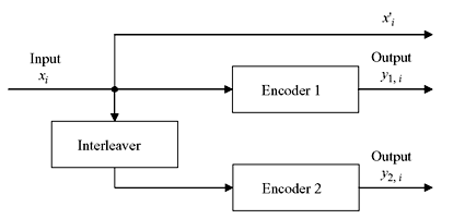
Figure 8.20 Turbo Code Generator

The key innovation of turbo codes is how they use the likelihood data to reconcile differences between the two decoders. Each of the two convolution decoders generates a hypothesis (with derived likelihoods) for the pattern of m bits in the payload sub-block. The hypothesis bit-patterns are compared, and if they differ the decoders exchange the derived likelihoods they have for each bit in the hypotheses. Each decoder incorporates the derived likelihood estimates from the other decoder to generate a new hypothesis for the bits in the payload. Then they compare these new hypotheses. This iterative process continues until the two decoders come up with the same hypothesis for the m-bit pattern of the payload, typically in 15–18 cycles.

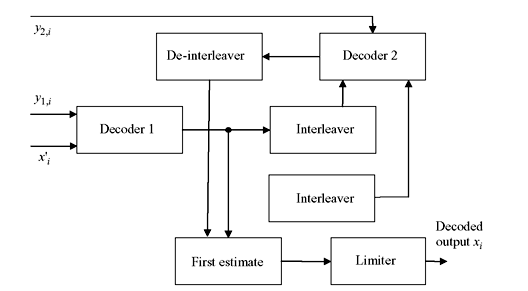
Figure 8.21 Turbo Decoder

Although the encoder determines the capability for the error correction, actual performance is determined by the decoder especially the algorithm used. Turbo decoding is an iterative process based on soft output algorithm like maximum a posteriori (MAP) or soft output Viterbi algorithm (SOVA). Soft output algorithm out-performs hard decision algorithms because soft output algorithm yields gradient of information about the computed information bits rather than just choosing a 1 or 0, resulting better estimate. The schematic of a turbo decoder is shown in Figure 8.21.

MAP algorithm is preferred to estimate the most likely information bit due to its better performance at low SNR conditions. However, it is complex enough as it focuses on each individual bit of information. Turbo decoding employs the iterative technique where the decoding process begins with receiving of partial information from x_i and y_1,i at the first decoder. The first decoder makes an estimate of transmitted signal and interleaves to match the format of y_2,i which is received by the second decoder. The second decoder now estimates based on the information from first decoder and the channel feeds back to first decoder for further estimation. This process is continued till certain conditions are met and the output taken out.

MAP or maximum a posteriori algorithm may be explained as a minimum probability of error rule. The general expression for the MAP rule in terms of a posteriori probability (APP) is as follows. Let x be the continuous valued random variable, P(d = i | x) is the APP for d = i representing the data d belonging to the ith signal class from a set of M classes, P(d = i) is a priori probability (the probability of occurrence of the ith signal class and p(x | d = i) is the probability density function (PDF) of received data with noise.

and

If binary logical elements 1 and 0 (representing electronic voltages +1 and –1, respectively) are transmitted over AWGN channel, Figure 8.22 represents the conditional PDFs referred to as likelihood functions. The transmitted data bit is d and the test statistic variable x observed at time kth time interval is x_k, yielding two likelihood values l₁ = p(x_k | d_k = +1) and l₂ = p(x_k | d_k = –1). The well-known hard decision rule chooses the data d_k = +1 or –1 depending on larger of l₁ and l₂. This leads to likelihood ratio test that decision will be taken depending 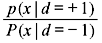on is greater or less than 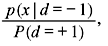alternatively, 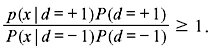By taking the logarithm of likelihood ratio we obtain the log-likelihood ratio (LLR) as follows:

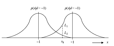
Figure 8.22 Conditional PDFs for –1 and + 1

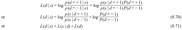
where L(x | d) is LLR of test statistic x obtained by measurement of the channel output x under alternate conditions d = +1 or d = –1 may have been transmitted and L(d) is the priori LLR of the data bit d. If decoder extrinsic LLR L_e(d) is considered, then after modification of Eq. (8.71), LLR of decoder output will be

 

 

The sign of L(d | x) decides hard decision of logical elements 1 or 0. The value of L_e(d) acts improvement of reliability of L(d | x). In the iterative process, initially the term (d) = 0, the channel LLR value L(x | d) = L_c(x) is measured according the values of L₁ and L₂ for a particular observation. The extrinsic LLR L_e(d) is fed back to input to serve as a refinement of the priori probability of the data for the next iteration.

At high SNR, the performance of turbo code is dominated by the free distance of it. In this region, the iterative decoder converges rapidly within after two to three iterations. The performance in this region usually improves slowly with increasing SNR. At low to moderate SNR, there is a sharp drop in BER and relatively large number of iterations is required for convergence. At very low SNR, number of iteration increases providing gain in performance. The overall code performance which is poor at BER is certainly beyond the normal operating region for most communication systems. Turbo codes are used extensively in the following telecommunication systems.

• 3G and 4G_–mobile telephony standards, e.g., in HSPA, EV-DO, and LTE.
• Media FLO, terrestrial mobile television system from Qualcomm.
• The interaction channel of satellite communication systems, such as DVB-RCS.
• New NASA missions such as Mars Reconnaissance Orbiter now use turbo codes, as an alternative to RS-Viterbi codes.
• Turbo coding, such as block turbo coding and convolution turbo coding, is used in IEEE 802.16 (WiMAX), a wireless metropolitan network standard.

8.10  INTERLEAVING TECHNIQUES: BLOCK AND CONVOLUTION

Wireless mobile communication channel as well as ionosphere and tropospheric propagation suffers from the phenomena of exhibiting mutually dependent signal impairments and multipath fading where signals arrive at the receiver over two or more paths of different lengths. The effect is that signals received are out of phase and distorted. These types of channels are said to have memory. Also some channels suffer from switching noise and other burst noise. All of these time-correlated impairments result in statistical dependence among successive symbol transmissions, i.e., burst errors. These errors are no longer characterized as single randomly distributed independent bit errors. Most block and convolution codes are designed to combat random-independent errors. But error performance for such coded signals is degraded in the channels with memory. Interleaving or the time diversity technique is adopted to improve the error performance, which requires the knowledge of the duration or span of the channel memory.

Interleaving the coded message before transmission and de-interleaving after reception causes bursts of channel errors to spread out in time and decoder handles them as random errors. Since the channel memory decreases with time separation in all practical cases, the idea behind interleaving is to separate code word symbols in time. The interleaving time is filled with the symbols of other code words. Separating the symbols in time, a channel with memory is effectively transformed to a memoryless channel and thereby enables the random-error-correcting codes to be useful in the channel with memory.

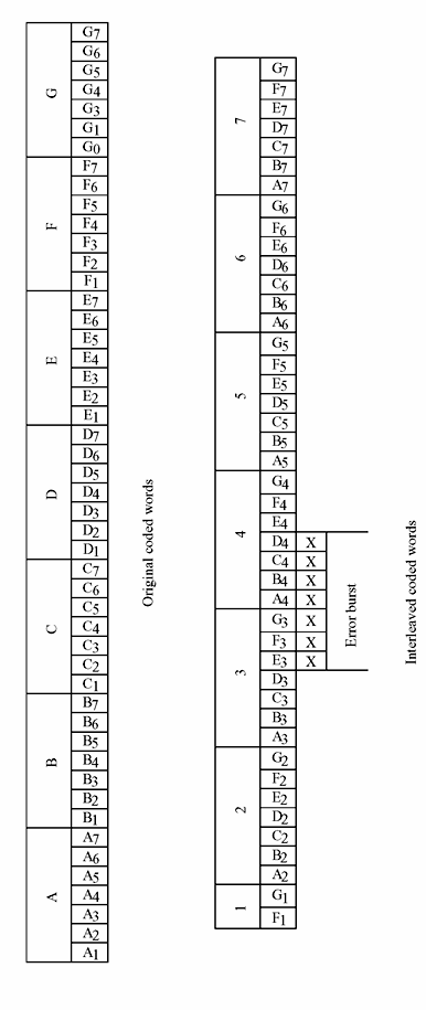
The interleaver shuffles the code symbols over a span of several block lengths or several constraint lengths. Span is determined by the burst duration. The detail of bit distribution pattern must be known to the receiver for proper extraction of data after deinterleaving. Figure 8.23 illustrates a simple interleaving example, where uninterleaved code words A to G, each code word comprising of seven code symbols. If the code word is of single-error-correcting capability and channel memory span is of one code word duration then the channel noise burst can destroy one or two code words. However, encoded data with interleaving can be reconstructed, though it is contaminated by burst noise. From Figure 8.23, it is clear that when the encoded data is interleaved and the memory span is enough to store one code word, though one code word is may be destroyed (as shown by xxxxxxx in the figure), this can be recovered from the seven code words after de-interleaving and decoding at the receiver end. Two types of interleavers are commonly used: (1) block interleavers and (2) convolution interleavers.

Block Interleavers—In this technique, the encoded code word of N code words, each of the M symbols, is fed to the interleaver in blocks columnwise to fill M × N array. After the array is completely filled, the output is taken out rowwise at a time, modulated and transmitted over the channel. At the receiver side, de-interleaver performs the reverse operation. Symbols are entered into the de-interleaver array through rows and taken out through columns. A 6 × 4 interleaving action is illustrated in Figure 8.24.

The most important characteristics of block interleaver are described as follows:

1. Any burst of less than N contiguous channel symbol errors results in isolated errors at the de-interleaver output which are separated from each other by at least M symbols.
2. Any bN burst of errors, where b > 1, results in the output burst from de-interleaver of no more than b₁ symbol errors. Each output burst is separated from the other bursts by no less than M − b₂ symbols, where b₁ is the smallest integer no less than b and b₂ is the largest integer less than b.
   

   Figure 8.23 Example of Interleave Operation

   

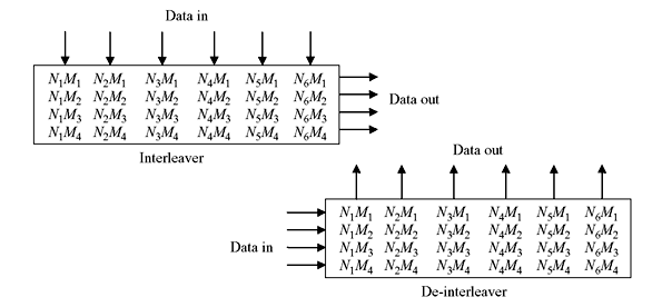
   Figure 8.24 Block Interleaver/De-interleaver Action

3. A periodic sequence of single errors spaced N symbols apart causes single burst of errors of length M at the de-interleaver output.
4. The interleaver/de-interleaver end-to-end delay is approximately 2MN symbol times. M(N − 1) + 1 memory cells are required to be filled before the commencement of transmission as soon as the first symbol of last column of M × N array is filled. A corresponding number is to be filled at the receiver before decoding begins. Thus minimum end-to-end delay is 2MN − 2M + 2 symbol times excluding the channel propagation delay.
5. Interleaver or de-interleaver memory requirement is MN symbols for each location. Since M × N array needs to be filled before it can be read out, memory of 2MN is generally implemented at each location.

Typically, the interleaver parameters are selected such that for single-error-correcting code the number of columns N is larger than expected burst length. The choice of number of rows M is dependent on the coding scheme. M should be larger than the code block length for block codes, while for convolution codes M should be greater than constraint length. Thus, a burst of length N can cause at most one single error in any block code word or in any constraint length for convolution codes. For t-error-correcting codes, N should be selected as greater than the expected burst length divided by t.

Convolution Interleavers—This type of interleaver uses N number of registers where code symbols are sequentially shifted. Each successive register has the storage capacity of J symbols more than the previous one. The zeroth register provides no storage, i.e., the symbol is transmitted immediately. Each new code symbol is fed to the new register as well as the commutator switches to this register. The new code symbol is shifted in while the oldest code symbol in that register is shifted out to modulator or transmitter. After the (N − 1)th register the commutator returns to zeroth register and the process continues.

The de-interleaver performs the same operation, but in reverse manner. Synchronization must be observed for both interleaver and de-interleaver. A schematic diagram of convolution interleaver and de-interleaver is shown in Figure 8.25 and an example of their timing action for four regiters is given in Figure 8.26. Initially at transmitter code word 1 is taken out directly. Code word 2 is fed to the register of J memory; code word 3 is fed to the register of 2J memory; and code word 3 to the register of 3J memory. Now the commutator switch returns to first position and receives next four code words in similar sequence. This process continues. The register contents and the output of interleaver are shown at the left side of Figure 8.26.

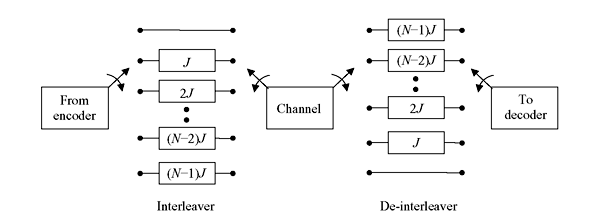
Figure 8.25 Convolution Interleaver/De-interleaver

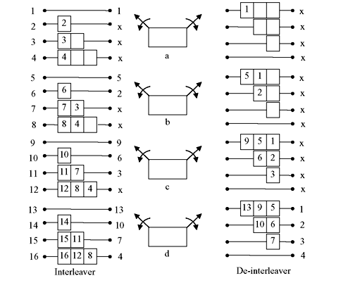
Figure 8.26 Convolution Interleaver/De-interleaver with Register Contents

In the receiver side, code word 1 is received first at the register of 3J memory and so there is no immediate output from de-interleaver. Next data is received at the register of 2J memory and the subsequent data at register of J memory while the following data is received directly. But there is no immediate valid output from de-interleaver. Now, the commutator switch returns to first position and receives next four code words while the previous stored symbols shift to next position of corresponding shift registers. De-interleaver will deliver valid code words from 13th time unit as indicated in Figure 8.26.

The performance of a convolution interleaver is very similar to that of block interleaver. However, the convolution interleaver has the advantage that it has end-to-end delay of M(N − 1) symbol, where M = NJ, and the memory required M(N − 1) at both ends which are ½ of the block codes.

8.11  CODING AND INTERLEAVING APPLIED TO CD DIGITAL AUDIO SYSTEM

A standard for the digital storage and reproduction of audio signals, known as the compact disc (CD) digital audio system, was defined by Philips Corp of the Netherlands and Sony Corp of Japan in 1979. This CD system has the world standard for achieving fidelity of sound reproduction of far quality compared to any other available technique. A plastic disc 120 mm in diameter is used to store the digitalized audio waveform which is sampled at 44.1 kilosamples/s to provide a recorded bandwidth of 20 kHz; each audio sample is uniformly quantized to one of 2¹⁶ levels (16 bits/sample), resulting in a dynamic range of 96 dB and a total harmonic distortion of 0.005%. A single disc of playing time of approximately 70 min stores about 10¹⁰ bits in the form of minute pits that are optically scanned by a laser.

There are several sources of channel errors. Small unwanted particles or air bubbles in the plastic material or pit inaccuracies arising in manufacturing cause errors in reproduction. Fingerprints or scratches during handling also introduce errors. It is difficult to predict actual cause of damage of a CD, but in the absence of an accurate channel model, it is safe to assume that the channel mainly has a burst-like error behaviour, since a scratch or fingerprint will cause errors on several consecutive data samples. A concatenated error control scheme called the cross-interleave Reed-Solomon code (CIRC) is an important aspect of the system design contributing to the high-fidelity performance. The data are rearranged in time so that digits stemming from contiguous samples of the waveform are spread out in time. In this way, error bursts are made to appear as single random events as explained in the earlier sections on interleaving. The protection of digital information is provided by adding parity bytes derived in two R-S encoders. Error control applied to the compact disc depends mostly on R-S coding and multiple layers of interleaving.

In digital audio applications, occasional detected failures are not so serious because they can be concealed, but an undetected decoding error is very serious since it results in clicks. The CIRC error-control scheme in the CD system involves both correction and concealment of errors. The performance specifications for the CIRC comprises of capability of maximum corrected burst length of 4000 bits (or a 2.5-mm track length on the disc), maximum interpolated burst length of 12000 bits (8 mm of track length), sample interpolation rate of one sample in every 10 h at P_B = 10⁻⁴ and 1000 samples/min at P_B = 10⁻³, undetectable error samples or clicks of less than one in every 750 h at P_B = 10⁻⁴ and negligible at P_B = 10⁻³. From the specifications it would appear that the CD can endure much damage (e.g., 8-min holes punched in the disc) without any noticeable effect on the sound quality. The CIRC system achieves its error control by a hierarchy of the following techniques:

1. The decoder provides a level of error correction.
2. The decoder provides a level of erasure correction, when the error correction capability is exceeded.
3. If the erasure correction capability is exceeded, the decoder attempts to conceal unreliable data samples by interpolating between reliable neighbouring samples.
4. The decoder blanks out of mutes the system for the duration of the unreliable samples, if the interpolation capability is exceeded.

8.11.1  CIRC Encoding and Decoding

Figure 8.27 illustrates the basic CIRC encoder block diagram (within the CD recording equipment) and the decoder block diagram (within the CD player equipment). Encoder consists of the encoding and interleaving steps designated as Δ-interleave, C2 encode, D* interleave, C1 encode, and D interleave. The decoder steps, consisting of de-interleaving and decoding, are performed in the reverse order of the encoding steps and are designated as D de-interleave, C1 decode, D* de-interleave, C2 decode, and de-interleave. CIRC system is characterized by the following five steps that are illustrated:

1. Δ-interleave—Two frames are formed by separating even-numbered samples and odd-numbered samples in order to scramble uncorrectable but detectable byte errors. Thus the interpolation process is facilitated.
2. C2 Encode—Four R-S parity bytes are added to Δ-interleaved 24-byte frame, resulting in total of n = 28 bytes. This (28, 24) code is called the outer code.
3. D* Interleave—In this section, each byte is delayed a different length, thereby facilitating spreading errors over several code words. C2 encoding together with D* interleaving have the function of providing for the correction of burst errors and error patterns that the C1 decoder cannot correct.
4. C1 Encode—Four R-S parity bytes are added to the k = 28 bytes of the D* interleaved frame, resulting in a total of n = 32 bytes. Thus (32, 28) code is formed which is called the inner code.
5. D Interleave—The even bytes of a frame with the odd bytes of the next frame are cross-interleaved here. By this procedure, two consecutive bytes on the disc will always end up in two different code words. The correction of most random single errors and the detection of longer burst errors are performed upon decoding, this interleaving, together with the C1 decoding.

Each of the inner and outer R-S codes with (n, k) values (32, 28) and (28, 24) as explained above uses four parity bytes. The code rate of CIRC is (k₁/n₁) (k₂/n₂) = 24/32 = 3/4. The minimum distance is d_min = n − k + 1 = 5. The error-correcting capability t and erasure correcting capability ρ may be expressed as follows:

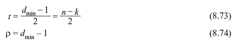
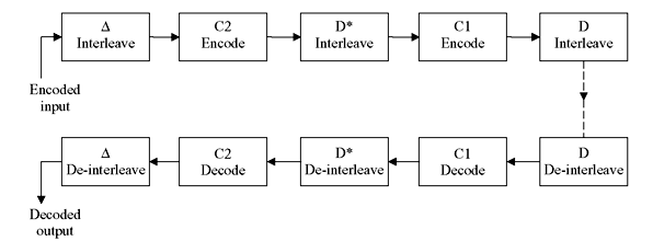
Figure 8.27 CIRC Encoder Block Diagram

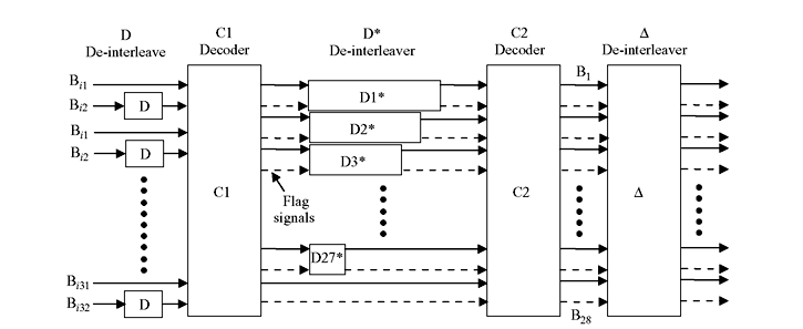
Figure 8.28 CIRC Decoder

It is possible to correct any pattern of α errors and γ erasures simultaneously provided that

 

 

Therefore, in above example, the scheme can correct two symbol errors and four symbol erasures per code word simultaneously. The decoding process is illustrated in Figure 8.28, where the processing is reverse manner.

1. D Interleave—Here 32 bytes of an encoded frame are applied to the 32 inputs of de-interleaver and every alternate byte of information is subjected to delay of one byte, so that even bytes are cross-de-interleaved with the odd bytes of next frame.
2. C1 Decode—The D de-interleaver and C1 decoder are designed to correct a single byte error in the block of 32 bytes. Larger burst errors are also detected here. However, multiple errors are passed unchanged through dashed lines attaching to all 28 remaining bytes with erasure flag. The parity bytes are no longer retained by C1 decoder.
3. D* De-interleave—Due to different lengths of de-interleaving delay lines, the errors that occurred in one word is spread over a number of words. Thus number of errors per unit word is reduced enabling C2 decoder to correct these errors.
4. C2 Decode—The burst errors that cannot be corrected by C1 decoder are corrected by C2 decoder. If C2 decoder cannot correct these errors, the 24-byte code word is passed unchanged to Δ-de-interleaver. Dashed output lines indicate the associated erasure flag.
5. Δ-De-interleave—The uncorrected but detected errors are finally corrected here by interpolation method using comparison with reliable neighbouring samples.

The output of C1 decoder consists of a sequence of 28-byte code words including extra one byte per code word for correction design. Each of the symbols in these code words is tagged with an erasure flag. Since a staggered delay is provided for each of the code words at D* de-interleave, the bytes of a give code word arrive in different code words at C2 decoder. C2 decoder is capable of four erasure corrections per code word and hence as many as four consecutive error bursts can be corrected. In the actual CD system, the delay increments are 4 byte, enabling maximum correction capability of 16 consecutive error bursts of C1 words.

8.11.2  Interpolation and Muting

Audible disturbances may be caused from the samples that cannot be corrected by the C2 decoder. The function of the interpolation process is to insert new samples, which is estimated from reliable neighbours, in place of the unreliable ones. It is impossible to apply interpolation without additional interleaving, if an entire C2 word is detected as unreliable, since both even and odd numbered samples are unreliable. This can happen if the C1 decoder fails to detect an error but the C2 decoder detects it. The purpose of Δ-de-interleaving is to obtain a pattern (over a span of two frame times) where even numbered samples can be interpolated from reliable odd numbered samples or vice versa. After de-interleaving, the unreliable samples are estimated by a first-order linear interpolation between neighbouring samples that stem from a different location on the disc.

In case of burst length exceeding 48 frames and two or more consecutive unreliable samples, another level of error control is provided in CD players. To combat this situation, the system is muted, i.e., audio is softly blanked out for a very small duration. If the muting time does not exceed a few milliseconds, it is not discernible to the human ear.

8.12  SOLVED PROBLEMS

Problem 8.1: Consider (3, 2, 1) convolution code of Figure 8.6. Find the composite generator polynomial g₁(D) and g₂(D). Find the code word for the input sequences u(D) = [1 + D + D³, 1 + D² + D³]

Solution: From the figure, the generator sequences are as follows:

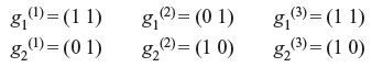
Therefore, G₁(D) = [1 + D, D, 1 + D] and G₂(D) = [D, 1, 1]. This can be written in composite form as follows:

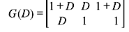
Input sequences u(D) = [1 + D + D³, 1 + D² + D³], i.e., u₁ = (1101) and u₂ = (1011).

The encoding sequences can be written as follows:

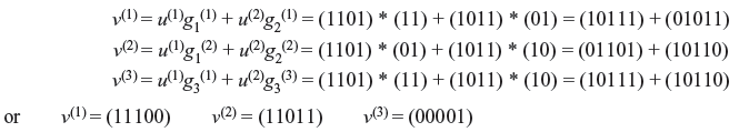
Therefore, output sequence or code word v = (110, 110, 100, 010, 011)

Code word may be written as v(D) = [1 + D, 1 + D, 1, D, D + D²]

Problem 8.2: The generator of (3, 1.5) systematic code are g⁽²⁾ = (110101) and g⁽³⁾ = (110011). Determine the generator polynomial and find the code word for information sequence u = (1101).

Solution:

The transfer function matrix is G(D) = [1, 1 + D + D³ + D⁵, 1 + D + D⁴ + D⁵]

As n = 3, the composite generator polynomial is

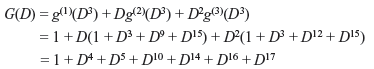
The information code word v(D) = u(D) G(D)

MULTIPLE CHOICE QUESTIONS

 

1. For (n, k, m) convolution code, k represents
   1. number of inputs 
   2. number of outputs
   3. number of memory 
   4. none of these

   Ans. (a)

2. An encoder for a (4, 3, 2) convolution code has the memory of order of
   1. 1 
   2. 2 
   3. 3 
   4. 4

   Ans. (b)

3. For a (4, 2, 3) convolution code of length L = 10, the fractional loss is
   1. 15.38% 
   2. 23.07% 
   3. 30.76% 
   4. 38.46%

   Ans. (b)

4. For generators g₁ = (1010) and g₂ = (1001) what is the output sequence of the input sequence u = (0110) after convolution coding?
   1. 00, 11, 10, 01, 11, 00, 11 
   2. 00, 10, 01, 11, 11, 00, 10
   3. 00, 11, 11, 10, 11, 01, 00 
   4. 00, 01, 10, 11, 00, 01, 10

   Ans. (c)

5. For a majority logic decoder, if number of orthogonal checksum and number of checked channel errors are 4 and 9, respectively, how many errors can be estimated correctly?
   1. 4 to 9 
   2. 2 to 9 
   3. 2 to 4 
   4. only 4

   Ans. (b)

6. Approximately what is the interleaver/de-interleaver end-to-end delay of 8 × 6 block interleaver?
   1. 6 symbol times 
   2. 8 symbol times
   3. 48 symbol times 
   4. 96 symbol times

   Ans. (d)

7. What is the error correction capability of CIRC code of inner and outer codes of (32, 28) and (28, 24)?
   1. 1 
   2. 2 
   3. 3 
   4. 4

   Ans. (b)

8. For convolution code, if s(D), H and e represent the syndrome, parity-check and error matrices the s^T(D) is
   1. H^Te 
   2. He^T 
   3. e^TH 
   4. eH^T

   Ans. (b)

9. Error control applied to the compact disc depends mostly on
   1. R-S coding 
   2. multiple layers of interleaving
   3. both of these 
   4. none of these

   Ans. (c)

REVIEW QUESTIONS

1. Define systematic code and noncatastrophic code.
2. Consider the (4, 3, 2) convolution code of Figure 8.7.
   1. Find the generator sequence.
   2. Find the generator matrix G.
   3. Find the code word for the message sequence (11101).
3. Considering (3, 2, 1) code of Figure 8.6, find the composite generator polynomial. If input sequences are (1101) and (1011), what will be the code word?
4. A (3, 1, 5) systematic code has generator sequences as (101101) and (110011). Find the generator matrix and parity sequence for the input sequence (1101).
5. Consider the (2, 1, 11) systematic code with g⁽²⁾ = 1 + D + D³ + D⁵ + D⁸ + D⁹ + D¹⁰ + D¹¹ has been subjected to majority logic decoder. Find the parity-check matrix. Write down the first constraint length of syndromes. How many channel errors can be estimated?
6. For (2, 1, 3) code with G(D) = [1 + D² + D³, 1 + D + D² + D³], draw the code tree. Find the code word if u = (1001).
7. For (2, 1, 3) code with G(D) = [1 + D² + D³, 1 + D + D² + D³] with Figure 8.5, draw the trellis diagram for length of 6.
8. Design a rate ½ convolution encoder with constraint length of 4 and minimum distance of 6. Construct the state diagram and trellis diagram of the encoder. What is the generator matrix of the code?
9. What are the advantages of Turbo code? Discuss how it is implemented.
10. What is interleaver? Discuss different types of interleaver. Also discuss the de-interleving process.
11. Compare the advantages and disadvantages of majority logic decoding, sequential decoding, and Viterbi decoding.
12. How the most likely path is decided for Viterbi decoding?