Table of Contents for

Information Theory, Coding and Cryptography

Chapter 5

Linear Block Codes

5.1  INTRODUCTION

With the advent of digital computers and digital data communication systems, information is coded in binary digits ‘0’ or ‘1’. This binary information sequence is segmented into message blocks of fixed length in block coding. Each message block consists of k-information bits and is denoted by u. Thus, there may be 2^k distinct messages. According to certain rules, this message u is then transformed into a binary n-tuple v, with n > k. The binary n-tuple v is referred to as the code vector (or code word) of the message u. Thus, there may be 2^k distinct code vectors corresponding to 2^k distinct possible message vectors. The set of these 2^k distinct code vectors is known as block code. A desirable property for block codes is linearity, which means that its code words satisfy the condition that the sum of any two code words gives another code word.

Definition 5.1: A block code c of length n consisting of 2^k code words is known as a linear (n, k) code if and only if the 2^k code words form a k-dimensional subspace of the vector space V_n of all the n-tuples over the field GF(2). 

It may be seen that in a binary linear code, the modulo-2 sum of any pair of code words gives another code word. Another very desirable property for a linear block code is to possess the systematic structure of the code as illustrated in Figure 5.1. Here the code word is divided into parts—the message part and the redundant checking part. The message part consists of k unaltered message digits, while the redundant checking part consists of (n – k) digits. A linear block code with this type of structure is referred to as a linear systematic block code. The structure may be altered; i.e., the message part of k digits can come first followed by (n – k) digits of redundant checking part.

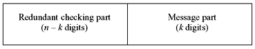
Figure 5.1 Systematic Form of a Code Word

5.2  GENERATOR MATRICES

From the definition of the linear code, we see that it is possible to find k linearly independent code words, g₀, g₁, g₂, ..., g_{k – 1}, in c such that every code word v in c is a linear combination of these k code words. Thus, it may be said that

where u_i = 0 or 1 for 0 ≤ i ≤ k. These k linearly independent code words may be arranged as the rows of a k × n matrix as follows:

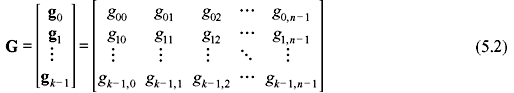
where g_i = (g_i0, g_i1, g_i2, …, g_{i,n – 1}) for 0 ≤ i ≤ k. Let us consider the message to be encoded is u = (u₀, u₁, u₂, …, u_{k – 1}). Thus, the corresponding code word is given as follows:

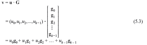
Thus, the rows of G generate the (n, k) linear code c. Hence, the matrix G is known as generator matrix for c. A point to be remembered is that any k linearly independent code words of c can be used to form a generator matrix.

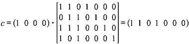
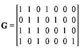
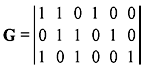
Example 5.1: Determine the set of code words for the (7, 4) code with the generator matrix

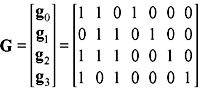
Solution: First we consider all the 16 possible message words (0 0 0 0), (10 0 0), (0 1 0 0), ..., (1 1 1 1). Substituting G and u = (1 0 0 0) into Eq. (5.3) gives the code word as follows:

Similarly, substituting all other values of u, we may find out the other code words. Just to illustrate the process, we find out another code word by substituting u = (1 1 1 1) which gives

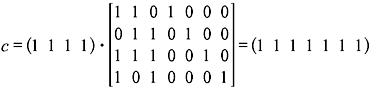
The total linear block code for the given generator matrix is shown in Table 5.1.

 

Table 5.1 The (7,4) Linear Block Code

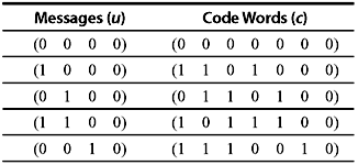
From Example 5.1, it is clear that the resultant code words are in systematic form, as the last four digits of each code word are actually the four unaltered message digits. This is possible since the generator matrix is in the form of G = [P   I₄], where I₄ is an 4 × 4 identity matrix. Thus, a linear systematic (n, k) code may be completely specified by a k × n matrix G of the following form:

where P_ij = 0 or 1. Thus, G = [P I_k] , where I_k denote the k × k identity matrix.

However, a generator matrix G may not necessarily be in a systematic form. In such a case, it generates a nonsystematic code. If two generator matrices differ only by elementary row operations, i.e., by swapping any two rows or by adding any row to another row, then the matrices generate the same set of code words and hence the same code. Alternatively if two matrices differ by column permutations then the code words generated by the matrices will differ by the order of the occurrence of the bits. Two codes differing only by a permutation of bits are said to be equivalent. It may be shown that every linear code is equivalent to a systematic linear code and hence every nonsystematic generator matrix can be put into a systematic form by column permutations and elementary row operations.

Example 5.2: A generator matrix the (5, 3) linear code is given by

Determine both the systematic and nonsystematic forms of the code words.

Solution: Here G is not of the systematic form (i.e., G ≠ [P    I_k]). To express G in systematic form, some elementary row operations have to be performed. It means we have to express G as G = [P   I₃], where I₃ is a 3 × 3 identity matrix and P is a 3 × 2 matrix. It is helpful to include a line in G showing where the matrix is augmented. To reduce G in systematic form, we first need to swap the positions of row 2 and row 3. This gives

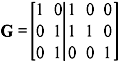
Then we add row 1 to row 2 to give

This is the required systematic form. Table 5.2 shows the resulting nonsystematic and systematic code words.

 

Table 5.2 The (5,3) Linear Block Code

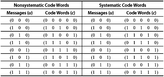
The code words generated by a systematic and a nonsystematic generator matrix of a linear code differ only in the mapping or correspondence between message words and code words. For example, the (5, 3) linear code with nonsystematic and systematic code words shown in Table 5.2 have the same set of code words but arranged in a different order. In both the cases, the mapping between the message words and code words is unique and hence either set of code words can be used to represent the message words. Thus, we can clearly see that a linear code does not have a unique generator matrix. Rather many generator matrices exist, all of which are equivalent and generate equivalent codes.

5.3  PARITY-CHECK MATRICES

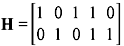
There is another very important matrix associated with every linear block code. We have already discussed in Chapter 4 that for any m × n matrix G, there exists an (n – m ) × n matrix H such that any vector in the row space of G is orthogonal to the rows of H. This is similarly true for the k × n generator matrix G discussed in this chapter. Thus, there exists an (n – k ) × n matrix H with vectors orthogonal to the vectors in G. This matrix H is known as the parity-check matrix of the code. Parity-check matrix is used at the decoding stage to determine the error syndrome of the code. This will be discussed in detail in the following section.

5.3.1  Dual Code

Since H is an (n – k ) × n matrix, the 2^{n – k} linear combinations of the rows can form an (n, n – k) linear code c_d. This code is the null space of the (n, k) linear code c generated by the matrix G. The code c_d is known as the dual code of c. Thus, it may be said that a parity-check matrix for a linear code c is the generator matrix for its dual code c_d.

If G of an (n, k) linear code is expressed in systematic form, the parity-check matrix H will be of the form:

 

 

Here P^T is the transpose of P and is hence an (n – k ) × k matrix and I_{n – k} is an (n – k ) × (n – k ) identity matrix. Thus, H may be represented in the following form:

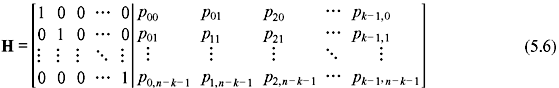
These (n – k) rows of H are linearly independent.

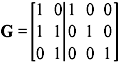
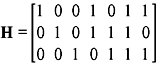
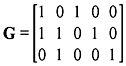
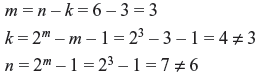
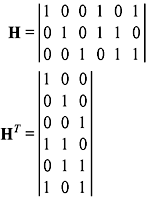
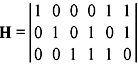
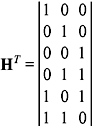
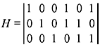
Example 5.3: Determine the parity-check matrix of the (7, 4) code with the generator matrix

Solution: The given generator matrix G for the (7, 4) code may be expressed as G = [P   I₄], where I₄ is a 4 × 4 identity matrix and

The transpose of P is given by

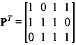
The parity-check matrix is expressed as H = [I₃   P^T], where I₃ is an 3 × 3 identity matrix.

Thus, H is given by

Since G = [P   I_k] and H = [ I_{n – k} P^T ], the product of G and the transpose of H of an (n, k) linear code is given by:

 

 

It is seen that [P   I_k] = P, where the order is [k × (n – k )] × (k × k) = k × (n – k ). Similarly, [ I_{n – k}   P^T] = P with order [(n – k ) × (n – k )] × [k × (n – k )] = k × (n – k ). Hence, from Eq. (5.7) we have

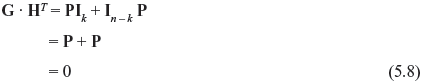
If there is an n-tuple v, which is a code word in c, we know v = u · G and multiplying this by H^T gives:

 

 

However, from Eq. (5.8), G · H^T = 0 and hence v · H^T = 0. Thus, for any linear code and parity-check matrix H, we have

 

 

Example 5.4: Determine the parity-check matrix H for the (5, 3) code. Show that G · H^T = 0 and v · H^T = 0 for v = (1 1 0 1 0 )

Solution: From the given generator matrix G, we get the parity matrix P as follows:

The parity-check matrix is given by H = [ I_{n – k}   P^T ], and hence

The product G · H^T gives

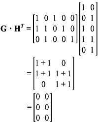
Thus, G · H^T = 0 as required.

Given v = (1 1 0 1 0). Hence,

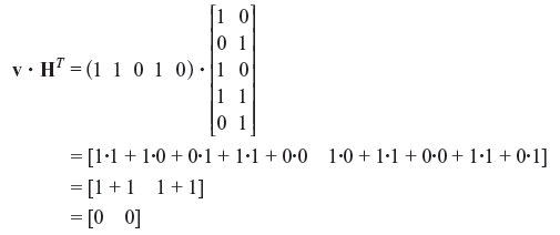
Hence, v · H^T = 0 as required.

5.4  ERROR SYNDROME

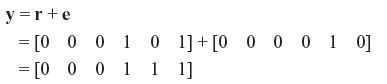
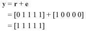
We consider an (n, k) linear code generated by the generator matrix G and having parity-check matrix H. Let us consider that v is a transmitted (n, k) code word over a channel and r is the corresponding received code word at the receiver end of the channel. If the channel is noisy then the received code word r may be different form the transmitted code word v. If we denote the received erroneous code word by the vector e, then it may be said that

 

 

Here e is also an n-tuple where e_i = 0 for r_i = v_i, and e_i = 1 for r_i ≠ v_i. This n-tuple vector e is also known as the error vector (or error pattern). The 1’s in e are the transmitted errors caused by the channel noise. From Eq. (5.10) it follows:

 

 

The receiver is unaware of either v or e. Hence, after receiving r, the decoder must first determine whether there is any transmission error within r. To do this, the decoder computes the (n – k) tuple as follows:

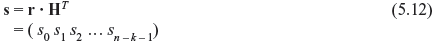
The vector s is called the syndrome of r. If there is no error (i.e., e = 0), then r = v (i.e., a valid code word) and s = 0 (since v · H^T = 0). On the other hand, if an error is detected (i.e., e ≠ 0), then r ≠ v. In such a case, s ≠ 0.

5.4.1  Undetectable Error Pattern

It may happen that the errors in certain vectors are not detectable. This happens if the error pattern e is identical to a nonzero code word. In such a case, r is the sum of two code words which is also another code word, and thus r · H^T = 0. This type of error patterns are known as undetectable error patterns. Thus, all valid nonzero code words become undetectable error patterns. Since there are 2^k – 1 valid nonzero code words, there are 2^k – 1 undetectable error patterns. Hence, when an undetectable error pattern occurs, the decoder makes a decoding error.

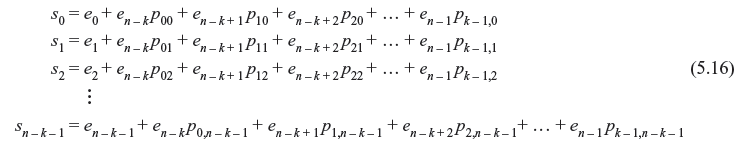
The syndrome digits may be computed from Eqs. (5.6) and (5.12) as follows:

Thus, from Eq. (5.13), we find that the syndrome s is simply the vector sum of the received parity digits (r₀, r₁, r₂, ..., r_{n – k – 1}) and the parity-check digits recomputed from the received message digits (r_{n – k}, r_{n – k + 1}, r_{n – k + 2}, … , r_{n – 1}).

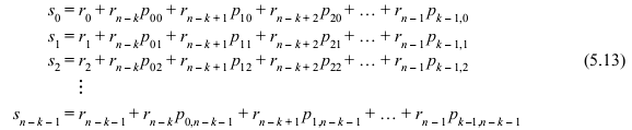
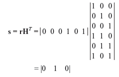
Example 5.5: Compute the error syndrome for the (7, 4) linear code whose parity-check matrix is similar to that computed in Example 5.3. Also design the syndrome circuit for the code.

Solution: Let us consider that r is the received 7-tuple vector. Then the syndrome s will be a 7 – 4 or 3-tuple vector. Let us denote s = (s₀, s₁, s₂ ). Hence, we have

Thus, the syndrome digits are

The syndrome circuit for the code is illustrated in Figure 5.2.

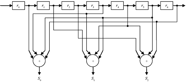
Figure 5.2 Syndrome Circuit for the (7,4) Linear Code of Example 5.5

Example 5.6: Assume that r₁ and r₂ represent two received code words of the (7, 4) linear code that have incurred errors. Compute the error syndromes of r₁ = (1 0 1 0 0 1 1) and r₂ = (1 1 1 1 0 0 0). The parity-check matrix is similar to that computed in Example 5.3.

Solution: Using the parity-check matrix for (7, 4) linear code similar to that computed in Example 5.3, we have the syndrome for the first received code word r₁ as follows:

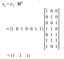
Similarly for r₂, we may compute the error syndromes as follows:

 

5.5  ERROR DETECTION

From Eqs. (5.11) and (5.12), it follows that

However, from Eq. (5.9) v · H^T = 0. Thus, we have the following relation between the error patterns and the syndrome:

 

 

Hence, we find that the syndrome s actually depends only on the error pattern e, and not on the transmitted code word v. Now if the parity-check matrix H is expressed by Eq. (5.6), then Eq. (5.15) gives

It may seem that by solving the (n – k) linear equations of (5.16), the error pattern e can be found out and therefore the vector (r + e) will be the actual transmitted code word v. The problem that arises in the (n – k) linear equations of (5.16) is that they do not have a unique solution but have 2^k solutions. Hence, there are 2^k error patterns which will result in the same syndrome. However, the true error patterns e is just one among them. Hence, the decoder has to determine the true error pattern from a set of 2^k error patterns. However, it is seen that if the channel is a BSC, the most probable error pattern is that which has the least number of 1’s. Thus, the decoder makes a choice of that error pattern which has smallest number of nonzero digits. Let us clarify it with an example.

Example 5.7: Assume that the actual code word sent over a BSC is v = (1 0 1 0 0 0 1). While received code word is r which is same as r₁ in Example 5.6. Correct the error occurred in the transmitted code word. The parity-check matrix is similar to that computed in Example 5.3.

Solution: From Example 5.6, we know that the computed syndrome for the received code word is s = (1 1 1). Now the receiver has to determine the true error pattern that may produce the computed syndrome. From Eqs. (5.15) and (5.16), we may write the equations relating the syndrome and error digits as follows:

Now there are 2⁴ = 16 error patterns that satisfy the above equations. They are as follows:

Since the channel is a BSC, the most probable error pattern is that which has the least number of 1’s. Hence, from the above 16 error patterns, we see that the most probable error pattern that satisfies the above equations is e₁ = ( 0 0 0 0 0 1 0). Thus, the receiver decodes the received vector r₁ as

We find that v′ is same as the transmitted code word v. Thus, the error has been corrected by the receiver.

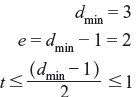
5.6  MINIMUM DISTANCE

In a block code, parity bits added with the message bits increase the separation or distance between the code words. The concept of distance between code words, and in particular the minimum distance within a code, is fundamental to error-control codes. This parameter determines the random-error-detecting and random-error-correcting capabilities of a code. The Hamming weight (or simply weight) of a binary n-tuple v is defined as the number of nonzero components of v and is denoted by w(v). For example, the Hamming weight of v = (1 1 0 0 1 1 1) is 5. The Hamming distance between two words v₁ and v₂, having same number of bits, is defined as the number of places in which they differ and is denoted by d(v₁, v₂).

For example, the code words v₁ = (1 0 1 0 0 0 1) and v₂ = (0 1 1 1 0 0 1) are separated in the zeroth, first, and third places and thus have Hamming distance of 3. Now the Hamming weight of the sum of v₁ and v₂ is as follows:

Thus, it may be written as follows:

 

 

It may be proved that the Hamming distance satisfies the triangle inequality. If v₁, v₂, and v₃ are the n-tuples in c, then

 

 

Definition 5.2: The minimum distance d_min of a block code c is the smallest distance between code words. Mathematically it is expressed as follows:

The minimum distance of a block code has the following property:

Property 1: The minimum distance of a linear block code is equal to the minimum weight of its nonzero code words. Mathematically it may be expressed as follows:

 

5.7  ERROR-DETECTING CAPABILITY

For a block code c with minimum distance d_min, it is obvious from Eq. (5.20) that there cannot remain any code word with weight less than d_min. Let a code vector v be transmitted over a noisy channel and be received as a vector r. Due to some error pattern within the channel, r is different from the transmitted vector v. If the error pattern is less than or equal to d_min – 1, then it cannot change one code vector to another, and hence the received vector r can in no way resemble a valid code word within c. Hence, the error will be definitely detected. Thus, it may be said that a block code c with minimum distance d_min is capable of detecting all error patterns of d_min – 1 or fewer errors. However, if the error pattern is of d_min errors, then this error pattern will change the transmitted code vector v into another valid code vector within c, since at least one pair of code vectors will exist which differs in d_min places. Hence, the error cannot be detected. The same argument applies for error patterns of more than d_min errors. Hence, it may be said that the random-error-detecting capability of a block code with minimum distance d_min is d_min – 1

At the same time, it may be seen that the block code with minimum distance d_min is also capable of detecting a large fraction of error patterns with d_min or more errors. For an (n, k) block code there are 2ⁿ – 1 possible error patterns. Among them there will be 2^k – 1 error patterns identical to 2^k – 1 nonzero code words. If any of these 2^k – 1 error patterns occurs, it alters the transmitted code word v into another valid code word w within the block. When w is received, the computed syndrome is zero, and the decoder accepts w as the transmitted code word. Hence, the decoder commits an incorrect decoding. Thus, these 2^k – 1 error patterns are undetectable. On the contrary, if the error pattern is not identical to any nonzero code word, then the received vector r cannot be a code word and hence the computed syndrome is nonzero. Thus, the error gets detected. Therefore, there will be 2ⁿ – 2^k error patterns which will not be identical to any of the code words of that (n, k) block code. These 2ⁿ – 2^k error patterns are detectable. In fact, an (n, k) linear code is capable of detecting 2ⁿ – 2^k error patterns of length n.

5.8  ERROR-CORRECTING CAPABILITY

The error correction capability of a block code c is determined by its minimum distance d_min. The minimum distance may either be even or odd. We consider that the code c can correct all error patterns of t or fewer bits. The relation between t and the minimum distance d_min is given as follows:

 

 

It may be proved that a block code with minimum distance d_min corrects all error patterns of t = (d_min – 1)/2 or fewer errors. The parameter (d_min – 1)/2 is known as random-error-correcting capability of the code. Hence, the code is referred as t error-correcting code.

At the same time t error-correcting code is usually capable of correcting many error patterns of t + 1 or more errors. In fact it may be shown that a t error-correcting (n, k) linear code is capable of correcting a total 2^{n – k} error patterns, which includes those with t or fewer errors.

5.9  STANDARD ARRAY AND SYNDROME DECODING

Let v₁, v₂, v₃, …, v₂k be the 2^k code vectors of the (n, k) linear code c. Irrespective of the code vector transmitted over a noisy channel, the received vector should be any of the 2ⁿ n-tuples. To develop a decoding scheme, all the possible 2ⁿ received vectors are partitioned into 2^k disjoint subsets d₁, d₂, d₃, …, d₂k. The code vector v_i is contained in the subset d_i for 1 ≤ i ≤ 2^k. Now if the received vector r is found in the subset d_i, r is automatically decoded into v_i.

Let us develop the method to partition all the possible 2ⁿ received vectors into 2^k disjoint subsets. This is done as follows:

1. Place all the 2^k code vectors of c in a row with the all-zero code vector v₁ = (0,0,0,...,0) as the first element.
2. From the remaining 2ⁿ – 2^k n-tuples, choose an n-tuple e₁ and place it under the zero code vector v₁.
3. Now fill in the second row by adding e₁ to each code vector v_i in the first row and place the sum v_i + e₁ under v_i.
4. Then another unused n-tuple e₂ is chosen from the remaining n-tuples and is placed under v₁.
5. Form the third row, by adding e₂ to each code vector v_i in the first row and placing the sum v_i + e₂ under v_i.
6. Continue this process until all the n-tuples are used.

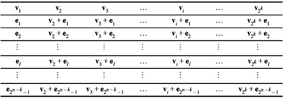
Thus, an array of rows and columns is constructed as shown in Table 5.3. This array is known as a standard array. A very important property of standard array to remember is that two n-tuples in the same row of a standard array cannot be identical and every n-tuple appears in one and only one row. Hence, from the construction of the standard array it is obvious that there are 2ⁿ/2^k = 2^{n – k} disjoint rows, where each row consists of 2^k distinct elements.

 

Table 5.3 Standard Array for an (n, k) Linear Code

5.9.1  Coset and Coset Leader

Each row in the standard array is known as the coset of the code c and the first element of each coset is called the coset leader. Any element of a coset may be used as a coset leader.

Due to the noise over the channel, if the error pattern caused is identical to the coset leader, then the received vector r is correctly decoded to the transmitted vector v. But if the error pattern caused is not identical to a coset leader, then the decoding will be erroneous. Thus, it may be concluded that the 2^{n – k} coset leaders (including the all zero vector) are the correctable error patterns.

Hence, to minimize the probability of an error in decoding, the coset leaders should be chosen in such a way that they happen to be the most probable error patterns. For a BSC, error patterns with lower weight are more probable than those with higher weight. Hence, when a standard array is formed, each coset leader chosen is a vector of least weight from the remaining available vectors. This is illustrated in Example 5.8. Thus, a coset leader has the minimum weight in a coset. In effect, the decoding based on the standard array is the maximum likelihood decoding (or, minimum distance decoding).

In fact, it may be said that for an (n, k) linear code c with minimum distance d_min, all the n-tuples of weight t = (d_min – 1)/2 or less may be used as coset leaders of a standard array of c.

Example 5.8: Construct a standard array for the (5, 2) single-error-correcting code with the following generator matrix.

Solution: The four code words will be (0 0 0 0 0), (1 0 1 0 1), (1 1 1 1 0), and (0 1 0 1 1). These code words form the first row of the standard array (as shown in Table 5.4). The second row is formed by taking (1 0 0 0 0) as the coset leader. The row is completed by adding (1 0 0 0 0) to each code word.

 

Table 5.4 Standard Array for an (5,2) Linear Code

Rows 3, 4, 5, and 6 are constructed using (0 1 0 0 0), (0 0 1 0 0), (0 0 0 1 0), and (0 0 0 0 1), respectively, as the coset leaders. Till row 6, we find that six words of weight 2 have already been used. Hence, there are four words left with weight 2, namely (1 1 0 0 0), (1 0 0 1 0), (0 1 1 0 0), and (0 0 1 1 0). Any of these may be used to construct the seventh row. We have used (1 1 0 0 0). Finally, (1 0 0 1 0) is used to construct the last row.

We have discussed that the syndrome of an n-tuple is an (n – k)-tuple. There are 2^{n – k} distinct (n – k)-tuples. There is a one-to-one correspondence between a coset and an (n – k)-tuple syndrome. It may be said there is a one-to-one correspondence between a coset leader and a syndrome. If we use this one-to-one correspondence relationship, a much simpler decoding table compared to a standard array may be formed. The table will consist of 2^{n – k} distinct coset leaders and their corresponding syndromes. Such a table is known as lookup table. In principle, this technique can be applied to any (n, k) linear code. This method results in minimum decoding delay and minimum error probability.

Using the lookup table, the decoding of a received vector follows the below-mentioned steps:

1. The syndrome of r is computed as r · H^T.
2. The coset leader e_i whose syndrome equals r · H^T is located. Then e_i is assumed to be the error pattern of the channel.
3. Finally, the received vector r is decoded as v = e_i + r.

However, it is to be noted that for large n – k, this scheme of decoding becomes impractical. In such case, different other practical decoding schemes are used.

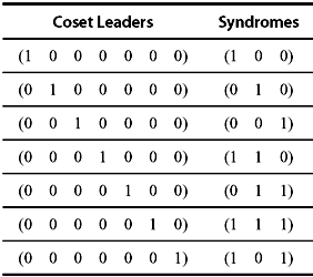
Example 5.9: Construct the lookup table for the (7, 4) linear code as given in Table 5.1. The parity-check matrix is determined in Example 5.3 and is given as follows:

Solution: The code will have 2³ = 8 cosets. Thus, there are 8 correctable error patterns which include the all zero vector.

The minimum distance of the code is 3. Hence, it is capable of correcting all error patterns of weight 1 or 0. Thus, all the 7-tuples of weight 1 or 0 can be used as coset leaders. Hence, the lookup table may be constructed as shown in Table 5.5.

 

Table 5.5 Lookup Table

5.10  PROBABILITY OF UNDETECTED ERRORS OVER A BSC

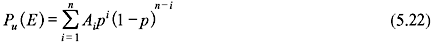
For an (n, k) linear code c, if n is large, then undetectable error patterns 2^k – 1 is much smaller compared to 2ⁿ. Thus, only a small fraction of error patterns remain undetected. We can find the probability of undetected errors from the weight distribution of c. Let there be A_i number of code vectors having weight i in c. Let the weight distribution of c be {A₀, A₁, A₂, … A_n} Let us denote the probability of an undetected error pattern as P_u(E). We know that an error pattern remains undetected when the error pattern is identical to a nonzero code vector of c. Hence,

where p is the transition probability of the BSC. There exists an interesting relationship between the weight distribution of a linear code c and its dual code c_d.

Let us assume that {B₀, B₁, B₂, ..., B_n} be the weight distribution of the dual code c_d, which is represented in the polynomial form as follows:

where A(x) and B(x) are related by an identity known as MacWilliams identity, and is given as follows:

The polynomials A(x) and B(x) are known as the weight enumerators for the (n, k) linear code c and its dual code c_d. Hence, using MacWilliams identity, the probability of an undetected error for an (n, k) linear code c can be computed from the weight distribution of its dual code c_d also. Eq. (5.22) may be written as follows:

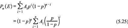
Putting x = p/(1 – p) in A(x) of Eq. (5.23) and using the fact that A₀ = 1 (since, there is only one all zero code), we obtain:

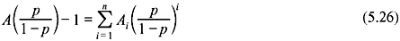
Combining Eqs. (5.25) and (5.26), we have:

Using Eqs. (5.27) and (5.24), we finally have:

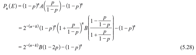
Therefore, we have two ways to calculate the probability of an undetected error for a linear code over a BSC. Generally if k is smaller than (n – k), it is easier to compute P_u(E) from Eq. (5.27); otherwise it is easier to use Eq. (5.28).

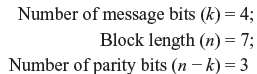
5.11  HAMMING CODE

Hamming codes have an important position in the history of error control codes. In fact, Hamming codes were the first class of linear codes devised for error control. The simplest Hamming code is the (7, 4) code that takes 4-bit information words and encodes them into 7-bit code words. Three parity bits are required, which are determined from the information bits.

For any positive integer m ≥ 3, there exists a Hamming code with the following parameters:

 

Code length:	n = 2m – 1
Information length:	k = 2m – 1 – m
Number of parity bits:	m = n – k
Error correcting capability:	t = 1 (for dmin = 3)

 

All the nonzero m-tuples will construct columns of the parity-check matrix H of this code. In systematic form, it may be written as follows:

 

 

where the submatrix Q consists of k columns which are the m-tuples of weight 2 or more and I_m is an m × m identity matrix.

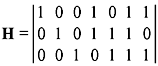
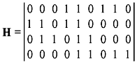
Here let us consider that m = 3. Then the parity-check matrix of the Hamming code of length 7 can be written as follows:

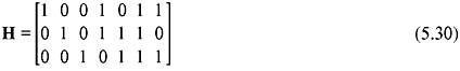
The parity-check matrix of the (7, 4) linear code is the same as given in Table 5.1. Thus, we conclude that the code shown in Table 5.1 is a Hamming code. Without affecting the weight distribution and the distance property of the code, the columns of Q may be arranged in any other order. Thus, the generator matrix of the code may be written in systematic form as follows:

 

 

Here Q^T is the transpose of Q and I_k is a k × k identity matrix.

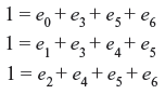
The columns of H are nonzero and distinct. Thus, no two columns of H can add up to zero. Hence, the minimum distance of a Hamming code is at least 3. Again as all the nonzero m-tuples form the columns of H, the vector sum of any two columns, say h_i and h_j, will be another column of H, say h_l. Hence,

 

 

This code can correct all the error patterns with a single error and can detect all the error patterns of two or fewer errors.

5.12  SOLVED PROBLEMS

Problem 5.1: Consider a (6, 3) linear block code defined by the generator matrix

 

1. Determine if the code is a Hamming code. Find the parity-check matrix H of the code in systematic form.
2. Find the encoding table for the linear block code.
3. What is the minimum distance d_min of the code? How many errors can the code detect? How many errors can the code correct?
4. Find the decoding table for the linear block code.
5. Suppose c = [0 0 0 1 1 1] is sent and r = [0 0 0 1 0 1] is received. Show how the code can correct this error.

Solution:

1. Testing for hamming code, we have
   

   Hence, (6, 3) is not a Hamming code.

   We have

   
2. The encoding table for (6, 3) linear block code is

   Message	Code Word	Weight of Code Word
   000	000000	0
   001	101001	3
   010	011010	3
   011	110011	4
   100	110100	3
   101	011101	4
   110	101110	4
   111	000111	3

3. From encoding table, we have
   

   Hence, the (6, 3) linear block code can detect two bit errors and correct one bit error in a 6-bit output code word.

4. We have
   

   The decoding table is

   Error Pattern	Syndrome	Comment
   000000	000	all 0’s
   100000	100	1st row of HT
   010000	010	2nd row of HT
   001000	001	3rd row of HT
   000100	110	4th row of HT
   000010	011	5th row of HT
   000001	101	6th row of HT

5. Given that c = [0 0 0 1 1 1] is sent and r = [0 0 0 1 0 1] is received.
   

   From decoding table, this syndrome corresponds to error pattern e = [0 0 0 0 1 0]. Hence, the corrected code word is

   

Problem 5.2: Consider a (5, 1) linear block code defined by the generator matrix

 

1. Find the parity-check matrix H of the code in systematic form.
2. Find the encoding table for the linear block code.
3. What is the minimum distance d_min of the code? How many errors can the code detect? How many errors can the code correct?
4. Find the decoding table for the linear block code (consider single bit errors only).
5. Suppose c = [1 1 1 1 1] is sent and r = [0 1 1 1 1] is received. Show how the code can correct this error.

Solution:

1. We have:  
   
2. The encoding table for (5, 1) linear block code is

   Message	Code Word	Weight of Code Word
   0	00000	0
   1	11111	5

3. From encoding table, we have
   

   Hence, the (5, 1) linear block code can detect four bit errors and correct two bit errors in a 5-bit output code word.

4. We have
   

   The decoding table is

   Error Pattern	Syndrome
   00000	0000
   10000	1000
   01000	0100
   00100	0010
   00010	0001
   00001	1111

5. Given that c = [1 1 1 1 1] is sent and r = [0 1 1 1 1] is received.
   

   From decoding table, this syndrome corresponds to the error pattern e = [1 0 0 0]. Hence, the corrected code word is

   

Problem 5.3: Construct the syndrome table for the (6, 3) single-error-correcting code, whose parity-check matrix is given by

Solution: Block length of the code = 6.

The transpose of H is

Hence, the error syndrome table is

Error Pattern	Syndrome
000000	000
100000	100
010000	010
001000	001
000100	011
000010	101
000001	110

Problem 5.4: Consider the following code vectors:

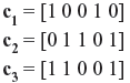
1. Find d(c₁,c₂), d(c₂,c₃), and d(c₁,c₃).
2. Show that d(c₁,c₂) + d(c₂,c₃) ≥ d(c₁,c₃).

Solution:

1. We know:
   

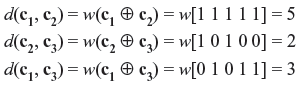
2. Now,

    

   d(c₁, c₂) + d(c₂, c₃) = 5 + 2 ≥ 3 = d(c₁, c₃)

Problem 5.5: Construct the eight code words in the dual code for the (7, 4) Hamming code and also find the minimum distance of this dual code. The parity matrix is

Solution: Parity-check matrix is

For a (7, 4) dual code H is used as a generator matrix.

Hence, code vector C_D = mH

Message	Code Word	Hamming Weight
000	0000000	0
001	0010111	4
010	0101110	4
011	0111001	4
100	1001011	4
101	1011100	4
110	1100101	4
111	1110010	5

The minimum value of the Hamming weight defines the Hamming distance of the dual code as follows:

 

MULTIPLE CHOICE QUESTIONS

1. The Hamming distance between v = 1100001011 and w = 1001101001 is
   1. 1 
   2. 5 
   3. 3 
   4. 4

   Ans. (d)

2.  Consider the parity-check matrix and the received vector r = (001110). Then the syndrome is given by
   1. (110)
   2. (100)
   3. (111) 
   4. (101)

      Ans. (b)

3. The number of undetectable errors for an (n, k) linear code is
   1. 2^{n – k} 
   2. 2ⁿ 
   3. 2ⁿ – 2^k 
   4. 2^k

      Ans. (d)

4. (7, 4) Hamming codes are
   1. single-error-correcting codes
   2. double-error-correcting codes
   3. burst-error-correcting codes 
   4. triple-error-correcting codes

   Ans. (a)

5. The condition of a dual code in case of linear block code is
   1. GH^T = 0 
   2. (GH)^T = 0 
   3. G^TH^T = 0 
   4. HG^T = 0

   Ans. (a)

6. A code is with minimum distance d_min = 5. How many errors can it correct?
   1. 3 
   2. 2 
   3. 4
   4. 1

   Ans. (b)

7. Check which code is a linear block code over GF(2).
   1. {111, 100, 001, 010} 
   2. {00000, 01111, 10100, 11011}
   3. {110, 101, 001, 010} 
   4. {0000, 0111, 1000, 1101}

   Ans. (b)

8. The_______between two words is the number of differences between corresponding bits
   1. Hamming code
   2. Hamming distance
   3. Hamming rule 
   4. none of the above

      Ans. (b)

9. To guarantee the detection of up to five errors in all cases, the minimum Hamming distance in a block code must be ________
   1. 5 
   2. 6 
   3. 11 
   4. 12

      Ans. (b)

10. To guarantee correction of up to five errors in all cases, the minimum Hamming distance in a block code must be ________.
    1. 5 
    2. 6 
    3. 11 
    4. 12

       Ans. (c)

11.  In a linear block code, the ______ of any two valid code words creates another valid code word.
    1. XORing 
    2. ORing 
    3. ANDing 
    4. none of these

       Ans. (a)

12. In block coding, if k = 2 and n = 3, we have ______ invalid code words.
    1. 8
    2. 4 
    3. 2
    4. 6

       Ans. (b)

13. The Hamming distance between equal code words is______.
    1. 1 
    2. n 
    3. 0 
    4. none of these

       Ans. (c)

14. In block coding, if n = 5, the maximum Hamming distance between the two code words is ________.
    1. 2 
    2. 3 
    3. 5 
    4. 4

       Ans. (c)

15. If the Hamming distance between a dataword and the corresponding code word is three, there are _______bits in the error.
    1. 3 
    2. 4 
    3. 5 
    4. 2

       Ans. (a)

16. The binary Hamming codes have the property that
    1. (n, k) = (2^m + 1, 2^m – 1 – m) 
    2. (n, k) = (2^m + 1, 2^m – 1 + m)
    3. (n, k) = (2^m – 1, 2^m – 1 – m) 
    4. (n, k) = (2^{m – 1} , 2^{m – 1} – m)

       Ans. (c)

17. A (7, 4) linear block code with minimum distance guarantees error detection of
    1. ≤ 4 bits 
    2. ≤ 3 bits 
    3. ≤ 2 bits 
    4. ≤ 6 bits

       Ans. (c)

Review Questions

1.  What is the systematic structure of a code word?
2.  Show that C = {0000, 1100, 0011, 1111} is a linear code. What is its minimum distance?
3.  What is standard array? Explain how the standard array can be used to make correct decoding.
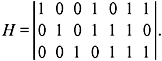
4.  What is syndrome and what is its significance? Draw the syndrome circuit for a (7, 4) linearblock code with parity-check matrix
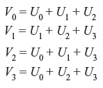
5. Consider a systematic (8, 4) code with the following parity-check equations
   

   where U₀, U₁, U₂, and U₃ are messages, V₀, V₁, V₂, and V₃ are parity-check digits.

   1. Find the generator matrix and the parity-check matrix for this code.
   2. Find the minimum weight for this code.
   3. Find the error-detecting and the error-correcting capability of this code.
   4. Show with an example that the code can detect three errors in a code word.
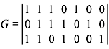
6. A (7, 3) linear code has the following generator matrix:
   

   Determine a systematic form of G. Hence, find the parity-check matrix H for the code.
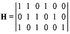
   Design the encoder circuit for the above code.

7. A code has the parity-check matrix
   

   Assuming that a vector (111011) is received, determine whether the received vector is a valid code. If ‘not’ determine what is the probable code vector originally transmitted. If ‘yes’ conform.

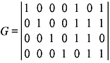
8. The generator matrix for a (7, 4) block code is given:
   
   1. Find the parity-check matrix of this code.
   2. If the received code word is (0001110), then find the transmitted code word.
9. Consider the (7, 4) linear block code whose decoding table is given as follows:

   Syndrome	Coset Leader
   100	1000000
   010	0100000
   001	0010000
   110	0001000
   011	0000100
   111	0000010
   101	0000001

   Show with an example that this code can correct any single error but makes a decoding error when two or more errors occur.

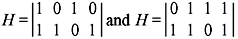
10. A (7, 3) code C has the following parity-check matrix with two missing columns.
    

    Provide possible bits in the missing columns given that [0110011] is a code word of C and the minimum distance of C is 4.

11. A code C has generator matrix
    
    1. What is the minimum distance of C?
    2. Decode the received word [111111111111].
12. A code C has only odd-weight code words. Say ‘possible’ or ‘impossible’ for the following with reasons.
    1. C is linear.
    2. Minimum distance of C is 5.
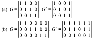
13. Show that, in each of the following cases, the generator matrices G and G′ generate equivalent codes.
    
14. If C is a linear code with both even and odd-weight code words, show that the number of even-weight code words is equal to the number of odd-weight code words. Show that the even-weight code words form a linear code.
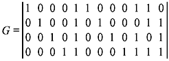
15. Consider two codes with parity-check matrices
    

    respectively.

    1. List all code words of the two codes.
    2. Provide G and H in systematic form for both codes.
16. Suppose that all the rows in the generator matrix G of a binary linear code C have even weight. Prove that all code words in C have even weight.
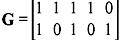
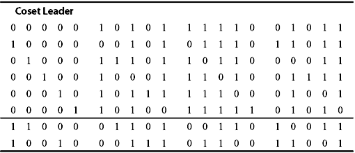
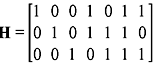
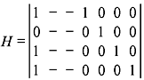
17. Let C be the binary [9, 5] code with parity-check matrix
    

    Find the coset leader(s) of the cosets containing the following words:

    1. 1 1 1 1 0 1 0 0 0
    2. 1 1 0 1 0 1 0 1 1
    3. 0 1 0 0 1 0 0 1 0.