Table of Contents for

Information Theory, Coding and Cryptography

Chapter 7

BCH Codes

7.1  INTRODUCTION

A large class of powerful random-error-correcting cyclic codes had been formed by BCH codes that made remarkable generalization of the Hamming codes for multiple error correction. BCH codes were invented in 1959 by Alexis Hocquenghem, and independently in 1960 by Raj Chandra Bose and Dwijendra Kumar Ray-Chaudhuri. Thus the code has been named as BCH (Bose Chaudhuri Hocquenghem) code. The cyclic structure of this code was observed and subsequently generalization of binary BCH codes to codes of p^m symbols (p is a prime) was done. However, in this chapter, the discussion will be confined to mainly binary BCH codes.

7.2  PRIMITIVE ELEMENTS

For any positive integers m (m ≥ 3) and t (t < 2^m – 1), there exist a BCH code with following parameters.

 

Block length:	n = 2m – 1
Number of parity-check digits:	n – k ≤ mt
Minimum distance:	dmin ≥ 2t + 1

 

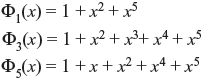
These features imply that this code is capable of correcting any combination of t or few numbers of errors in a block code n = 2^m – 1 digits and hence it is called t-error-correcting BCH code. The generator polynomial of this code is specified in terms of its roots from Galois field GF(2^m). If α is the primitive element of GF(2^m), then the generator polynomial g(x) of t-error-correcting BCH code of length 2^m – 1 is the lowest degree polynomial with the roots as α, α², α³, ..., α^2t and also the conjugates of them [i.e., g(αⁱ) = 0, for 1≤ i ≤ 2t]. If Φ_i(x) has the root as αⁱ, g(x) is least common multiple of Φ₁(x), Φ₂(x),…, Φ_2t(x), i.e., 

If i is even integer, this can be expressed as i = k2^l, where k is odd integer and l ≥ 1. Then αⁱ has a conjugate α^k, and hence αⁱ and α^k have same polynomial. Therefore, g(x) may be expressed as follows:

As the degree of each polynomial is m or less, the degree of g(x) is at most mt. From Eq. (7.2), the single-error-correcting code may be generated by g(x) = Φ₁(x).

Example 7.1: For n = 7 and k = 4, t = 1, this means single-error-correcting code may be generated. Similarly, for n = 15 and k = 11, t = 1 or this is also a single-error-correcting code. For n = 15, double error correction and 3-error correction can be achieved with k = 7 and k = 5, respectively.

7.3  MINIMAL POLYNOMIALS

If Φ(x) is the polynomial with the coefficients from Galois field GF(2^m), which is irreducible, it is called minimal polynomial. It has the degree ≤m and it divides x^2m + x. For example, the minimal polynomials of γ = α⁷ in GF(2⁴) is ɸ(x) = 1 + x³ +x⁴.

Minimal polynomials are obtained by solving the equation

 

 

where x is substituted by γ = α⁷ and m = 4 for GF(2⁴). The minimal polynomials generated by p(x) = x⁴ + x + 1 are given at Table 7.1.

 

Table 7.1 Minimal Polynomials in GF (2⁴) Generated by p(x) = x³ + x + 1

Conjugate Roots	Minimal Polynomials
0	x
1	x + 1
α, α2, α4, α8	x4 + x + 1
α3, α6, α9, α12	x4 + x3 + x2 + x + 1
α5, α10	x2 + x + 1
α7, α11, α13, α14	x4 + x3 + 1

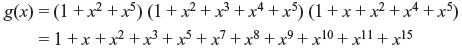
7.4  GENERATOR POLYNOMIALS

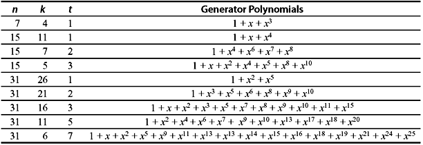
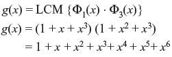
Using the minimal polynomials, Galois field of any order may be constructed and generator polynomials may be selected according to error-correction capability. A t-error-correcting BCH code, polynomial of code length of n = 2^m – 1 may be generated where each code polynomial has the roots α, α², α³, …, α^2t and their conjugates. Now if v(x) is the code polynomial from GF(2), it is divisible by the minimal polynomials Φ₁(x), Φ₂(x), …, Φ_2t(x). Therefore, v(x) is also divisible by their least common multiple or generator polynomial g(x), where g(x) = LCM {Φ₁(x) · Φ₂(x) · Φ₃(x) … Φ_2t(x)}. A list of generator polynomial of binary BCH codes of block length up to 2⁵ – 1 is given in Table 7.2.

 

Table 7.2 Generator Polynomials of BCH Code

If t-error-correcting code polynomial v(x) = v₀ + v₁x + v₂x² + … + v_n _ ₁x^{n – 1} of code length 2^m – 1 has the root αⁱ, then

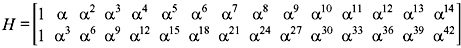
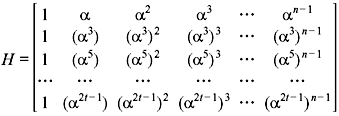
If we consider a matrix H consisting of the primitive elements that are the roots of the code vector as follows:

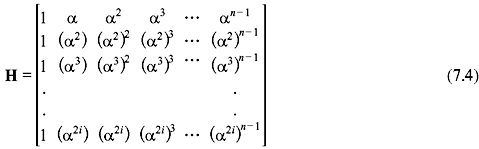
As v is a code vector, then v · H^T = 0.         (7.5)

The BCH code with minimum distance at least d₀ has no more than m(d₀ – 1) parity-check digits and capable of correcting (d₀ – 1)/2 or fewer errors. The lower bound on minimum distance is called the BCH bound.

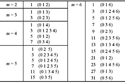
A list of primitive elements for minimal polynomials for 1< m ≤ 6 is given in Table 7.3.

 

Table 7.3 Primitive Elements of Minimal Polynomials

Example 7.2: If α be the primitive element of Galois field GF(2⁴), with 1 + α + α⁴ = 0, the minimal polynomials are

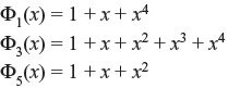
Double-error-correction BCH code of length n = 2⁴ – 1 = 15 is generated by

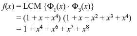
Thus, this code is (15, 7) cyclic code of d_min = 5.

Similarly, triple-error-correcting (15, 5) code with d_min = 7 may be generated by the generator polynomial

7.5  DECODING OF BCH CODES

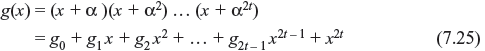
Let us consider that the transmitted code vector v(x) = v₀ + v₁x + v₂x² + … + v_n _ ₁x^{n – 1} is received as r(x) = r₀ + r₁x + r₂x² + … + r _n _ ₁x^{n – 1}. If e(x) is error introduced then

 

 

Syndrome vector can be calculated as

 

 

where H is given in Eq. (7.4). The ith component of syndrome is S_i = r(αⁱ), i.e., for 1≤ i ≤ 2t

 

 

It may be noticed that syndrome components are the elements in the field GF(2^m). Dividing r(x) by the minimal polynomial Φ_i(x) of αⁱ, we have r(x) = a_i(x)Φ_i(x) + b_i(x), where b_i(x) is the remainder with degree less than that of Φ_i(x). Now Φ_i(αⁱ) = 0, therefore

 

 

Thus the syndrome components may be obtained by evaluating b_i(x) with x = αⁱ. Since αⁱ is the root of each code polynomial and v(αⁱ) = 0, from Eqs. (7.6) and (7.9), for 1 ≤ i ≤ 2t, we may relate the syndrome components with the error pattern as follows:

 

 

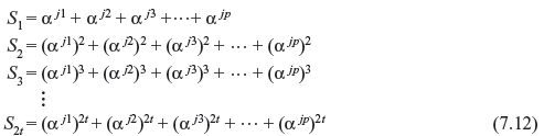
It may be noticed that syndrome components S_i depend on error pattern. Suppose there exists p number of errors in error pattern e(x) at locations x^j1, x^j2, ..., x^jp, we may write

 

 

where 0 < j1 < j2 < ... < jp < n. From Eq. (7.10), we may derive the following set of equations for S_i.

In the above set of equations, the roots α^j1, α^j2, α^j3, ..., α^jp are unknown. Solving these equations we may find the error locations. Any method for solving these equations is a decoding algorithm for BCH codes.

For convenience, α^jl is substituted by β₁, such that α^j1 = β_l for 0 < l < n. The elements β_l are called the error location numbers. Eq. (7.12) may be rewritten as follows:

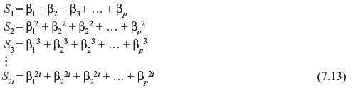
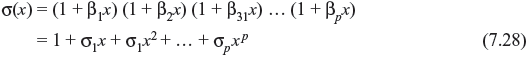
The above set of equations are symmetric functions of β₁, β₂, β₃, …, β_p, which are known as power-sum symmetric functions. Let us consider the following polynomial.

The roots of σ(x) are which are the inverse of the error location numbers, and therefore σ(x) is called as error location polynomial. σ₀, σ₁, σ₂, ..., σ_p are the elementary symmetric functions of β₁, β₂, β₃, ..., β_p. The coefficients of σ(x) can be computed as per following relations.

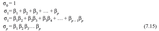
The σ₀, σ₁, σ₂, ..., σ_p are known as the elementary symmetric functions of β₁, β₂, β₃, ..., β_p. From Eqs. (7.13) and (7.15), we can relate the syndrome components by following Newton’s identities.

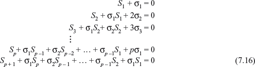
Solving the above equations for the elementary functions σ₀, σ₁, σ₂, ..., σ_p, we may find out the error locations β₁, β₂, β₃, ..., β_p. Eq. (7.16) may have many solutions. However, the solution that yields σ(x) of minimal degree is to be considered for determining the error pattern. If p ≤ t, σ(x) will give the actual error pattern e(x). Therefore, the error correction procedure for BCH codes may be described as follows:

• Computation of syndromes from the received polynomial r(x).
• Determining of error location polynomial σ(x) from syndrome components S₁, S₂, S₃, ..., S_2t.
• Finding the roots of σ(x) to determine the error location numbers β₁, β₂, β₃, ..., β_p and correction of errors in r(x).

Finding the error location polynomial σ(x) is most complicated and can be achieved by iterative process. The first step is to search a minimum degree polynomial σ⁽¹⁾(x) whose coefficients satisfy the first Newton’s identity of Eq. (7.16). In the next step, coefficients of σ⁽¹⁾(x) are tested to satisfy the second Newton’s identity of Eq. (7.16). If this satisfies, then σ⁽²⁾(x) = σ⁽¹⁾(x). If the coefficients of σ⁽¹⁾(x) do not satisfy the second Newton’s identity, a correction term is added to σ⁽¹⁾(x) to form σ⁽²⁾(x) such that σ⁽²⁾(x) has minimum degree and satisfies second Newton’s identity. Next σ⁽²⁾(x) is to be tested for third Newton’s identity equation. This iteration process is to be continued till all the Newton’s identity equations are tested and finally the error location polynomial will be obtained after 2tth iteration such that σ(x) = σ^(2t)(x).

Let the minimal degree polynomial at the μth step of iteration whose coefficients satisfy the first μ Newton’s identity equations be

To determine σ^{(μ + 1)}(x), we compute the following.

The quantity d_μ is called μth discrepancy. If d_μ = 0, the coefficients of σ^(μ)(x) satisfy the (μ + 1)th Newton’s identity and σ^{(μ + 1)}(x) = σ^(μ)(x). If d_μ ≠ 0, a correction term is to be added as stated earlier. To find the correction term, we have to consider the step prior to μth step, say ρth step, where ρth discrepancy d_ρ ≠ 0. If l_ρ is the degree of the polynomial σ^(ρ)(x), where ρ – lρ has the largest value, then

After completion of iterative method, the final error location polynomial σ(x) is determined. Now the error location numbers can be found simply by substituting 1, α, α², ..., α^{n – 1} (n = 2^m – 1) into σ(x) and subsequently the error pattern e(x) may be obtained. Therefore, the decoding process is to be performed on a bit-by-bit basis.

 

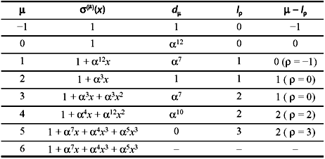
Example 7.3: Consider the (15, 5) triple-error-correcting BCH code in Galois field GF(2⁴) such that 1 + α + α⁴ = 0. Assume that the code vector v = (000000000000000) has been received as r = (000101000000100).

 

Therefore, 

 

 

The minimal polynomials of α, α², and α⁴ are identical and

 

 

The minimal polynomials for α³ and α⁶ are

 

 

The minimal polynomial for α⁵ is Φ₅(x) = 1 + x + x²

Dividing r(x) by above minimal polynomials, we obtain the remainders as follows:

 

 

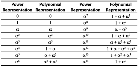
Substituting α, α², α⁴ in b₁(x), α³, α⁴ in b₃(x), and α⁵ in b₅(x), we obtain the syndrome components as S₁ = S₂ = S₄ = 1, S₃ = 1 + α⁶ + α⁹ = α¹⁰, S₆ = 1 + α¹² + α¹⁸ = α⁵, and S₅ = α¹⁰. These results are obtained from the polynomial representations of the elements of GF(2⁴) as in Table 7.4.

 

Table 7.4 Polynomial Representation of Elements of GF(2⁴)

To find the error location polynomial, the iterative method as described above is used. The steps and results of iterative process are indicated in Table 7.5. To begin the iterative process, for the first row, we assume μ = –1. Therefore, from Eqs. (7.17) and (7.18), σ^{(μ = –1)}(x) = 1, d_{μ = –1} = 1 and l_µ is the degree of σ^(μ)(x).

For the next row μ = 0, σ^{(μ = 0)}(x) = σ^{(μ = –1)}(x) = 1 as d_{μ= –1} = 0. Now d_{μ = 0} = S₁ = 1 from Eq. (7.18). Thus, the iterative process continues to develop till μ = 2t. The algorithm maintained is as follows:

• If d _μ = 0, σ^{(μ + 1)}(x) = σ^(μ)(x) and 1_{μ + 1} = l_μ.
• If d_μ ≠ 0, another row to be found prior to μth, say ρth, such that ρ – l_ρ is maximum and d_ρ ≠ 0.

  Then, σ^(μ + ¹⁾(x) is computed as from Eq. (7.19). In either case

  
• If polynomial σ^2t(x) in the last row has the degree greater than t, there are more than t errors that cannot be located.

Table 7.5 Iterative Process to Find the Error Location

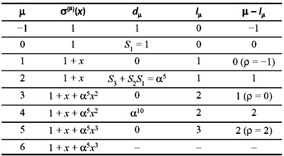
Thus, we obtain the error location polynomial

 

 

We can verify that α³, α¹⁰, and α¹² are the roots of above error location polynomial σ(x). The inverse of these roots are α¹², α⁵, and α³. Hence, the error pattern is e(x) = x³ + x⁵ + x¹². Adding e(x) with r(x) we can recover errorless code vector.

7.6  IMPLEMENTATION OF GALOIS FIELD

As discussed above, decoding of BCH codes requires computation using Galois field arithmetic that consists of mainly two operations—addition and multiplication. For addition operation, the resultant vector is the vector representation of the sum of the two field elements. The addition operation can be accomplished with circuit diagram shown in Figure 7.1.

Two elements are loaded in registers A(a₀, a₁, a₂, a₃) and B(b₀, b₁, b₂, b₃). Register A also serves as accumulator. The sum of two elements is available at the accumulator after applying triggering pulse to the adders.

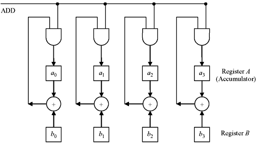
Figure 7.1 Schematic for Addition Operation

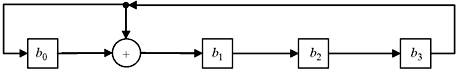
Figure 7.2 Multiplication Scheme of a Field Element with a Fixed Element

Multiplication of field element by a fixed element may be carried out using shift registers as shown at Figure 7.2. Let us consider the multiplication of field element B in GF(2⁴) by primitive element α whose minimal polynomial is Φ(x) = 1 + x + x⁴. The element B can be expressed as a polynomial with respect to α as B = b₀ + b₁α + b₂α² + b₃α³. Using the fact α⁴ = 1 + α, we obtain the equality, αΒ = b₃ + (b₀ + b₃)α + b₁α² + b₂α³, which can be realized by the circuit as shown in Figure 7.2.

Successive shifts of the shift register will generate the vector representation of successive powers of α according to the order in Galois field. If initially register is loaded with 1000, after 15th shift the register will contain 1000 again.

Now, let us consider the multiplication of two arbitrary field elements B and C, such that

 

 

The product BC may be written in the following form.

 

 

The steps of multiplication may be described as follows:

• Multiply c₃B by α and add to c₂B.
• Multiply (c₃B)α + c₂B by α and add to c₁B.
• Multiply [(c₃B)α + c₂B)α + c₁B by α and add to c₀B.

Multiplication by α can be performed by the circuit as shown in Figure (7.2). Overall computation for the multiplication of two field elements B and C can be carried out by the schematic circuit diagram as shown in Figure (7.3). Here, the field elements B and C are loaded in the register B and register C, respectively. Register A is initially empty. After four simultaneous shifts of registers A and C, the desired product is available in register A.

The received vector r(x) may be computed in similar way. Figure 7.4 demonstrate the computation of r(αⁱ), where α is the primitive element of GF(2⁴).

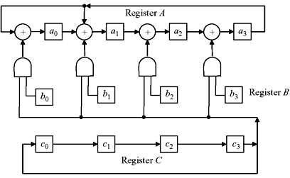
Figure 7.3 Multiplication Scheme for Two Field Elements

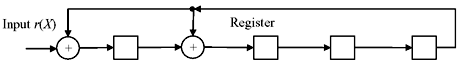
Figure 7.4 Computation of r(αⁱ)

The received polynomial r(α) may be written as follows:

After 15th shift at shift register shown in Figure 7.4, the register will contain r(α) in vector form. It may be noted that the figures explained for implementation of Galois field are not unique. Various circuits may be realized according to operator polynomials.

7.7  IMPLEMENTATION OF ERROR CORRECTION

As discussed earlier, corrected data at the receiver end require syndrome computation, error location polynomial search and error correction. These can be implemented either by digital hardware or by software programmed on a general purpose computer. The advantage of hardware implementation is faster computation; but software implementation is less expensive.

7.7.1  Syndrome Computation

Syndrome components S₁, S₂, ..., S_2t for t-error correction BCH code may be obtained by substituting the field elements α, α², ..., α^2t into the received polynomials r(x).

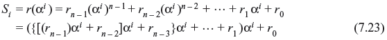
The computation consists of n – 1 additions and n – 1 multiplications which can be achieved by the hardware as described in Section 7.6. Since the generator polynomial is a product of at most t minimal polynomials, to form 2t syndrome components it requires at most t feedback shift registers, each containing at most m stages. It takes n clock cycles for complete computation. A syndrome computation circuit schematic for double-error-correcting (15, 7) BCH code is shown in Figure 7.5. As soon as the entire r(x) is received by the circuit, the 2t syndrome components are formed.

7.7.2  Computation of Error Location Polynomial

Since there are t numbers of error location polynomials σ^(μ)(x) and t numbers of discrepancies d_μ, computation of them requires 2t² additions and 2t² multiplications. Addition and multiplication circuits are already discussed which can be used to realize them. Figure 7.6 demonstrates Chein’s searching circuit, the schematic for finding the error locations.

Error location polynomial σ(x) of degree t is substituted by the field elements. Chein’s searching circuit consists of t multipliers for multiplying α, α², ..., α^t, respectively. Initially σ₁, σ₂, ..., σ_t are loaded into the registers of multipliers. After lth shift, these register will contain σ₁α^l, σ₂α^2l, ..., σ_tα^tl. The sum 1 + σ₁α^l + σ₂α^2l + … + σ_tα^tl is computed by m-input OR/NOR gate. If the sum is zero, the error location number is α^{n – 1}. It requires n clock cycles to complete this step and k clock cycles to correct only the message bits.

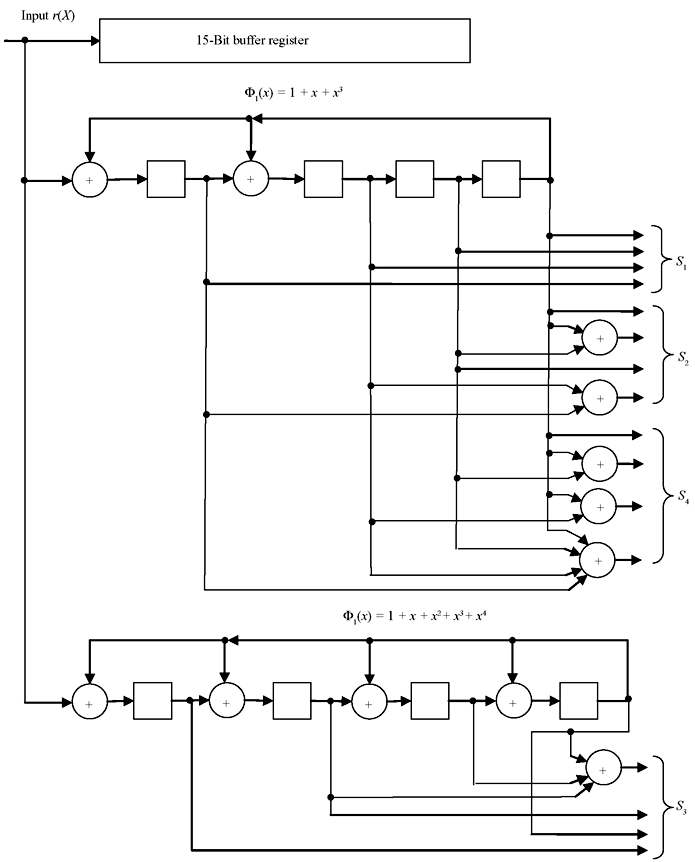
Figure 7.5 Syndrome Computation Circuit for Double Error Correcting (15,7) BCH Code

Figure 7.6 Chein's Error Searching Circuit

7.8  NONBINARY BCH CODES

Apart from binary BCH codes, there exist nonbinary codes in Galois field. If p is a prime number and q is any power of p (q = p^m), there are codes with symbols from the Galois field GF(q) which are called q-ary codes. The concepts and properties of q-ary codes are similar to binary code with little modification. An (n, k) linear code with symbols from GF(q) is a k-dimensional subspace of the vector space in GF(q). A q-ary (n, k) cyclic code is generated by a polynomial of degree n – k with coefficients from GF(q), which is a factor of xⁿ – 1. Encoding and decoding of q-ary codes are similar to that of binary codes.

For any choice of positive integers s and t, there exists a q-ary BCH code of length n = q^s – 1, which is capable of correcting any combination of t or fewer errors and requires no more than 2st parity-check digits. The generator polynomial g(x) of lowest degree with coefficients from GF(q) for a t-error-correcting q-ary BCH code, which has the roots α, α², ..., α^2t, may be generated from the minimal polynomials Φ₁(x), Φ₂(x), …, Φ_2t(x), such that

Each minimal polynomial has the degree s or less and hence the degree of g(x) is at most 2st and the number of parity-check digits of the code is no more than 2st. For q = 2, we obtain binary BCH code.

7.8.1  Reed-Solomon Code

Reed–Solomon code is one of the special subclass of q-ary BCH codes for which s = 1. A t-error-correcting Reed–Solomon code with primitive elements from GF(q) has the following parameters:

Block length:	n = q – 1
Number of parity digits:	n – k = 2t
Minimum distance:	dmin = 2t + 1

It may be noted that the length of this code is one less than the size of code symbols and minimum distance is one greater than the number of parity-check digits. For q = 2^m with α as the primitive elements in GF(2^m), the generator polynomial g(x) may be written as follows:

The code generated by g(x) is an (n, n – 2t) cyclic code consisting of the polynomials of degree n – 1 or less with coefficients from GF(2^m) that are multiples of g(x). Encoding of this code is similar to the binary BCH code. If the message polynomial a(x) = a₀ + a₁x + a₂x² + ... + a_{k – 1} x^{k – 1} + a_k x^k is to be encoded, where k = n – 2t, remainder b(x) = b₀ + b₁x + b₂x² + ... + b_{2t – 1}x^{2t – 1} is obtained dividing x^2ta(x) by g(x). This can be accomplished by the schematic circuit as shown in Figure 7.7.

Here, the adders denotes the addition of two elements from GF(2^m) and multipliers perform multiplication of field element from GF(2^m) with a fixed element g_i from the same field. Parity digits will be generated in the registers as soon as the message bits entered in the circuit.

Decoding of Reed–Solomon code is performed in similar process as described for binary BCH code. Decoding of this code consists of four steps: (1) computation of syndrome, (2) determining error location polynomial σ(x), (3) finding the error location numbers, and (4) evaluation of error values. The last step is not required in binary BCH code. If r(x), v(x), and e(x) are the received, transmitted, and error polynomials, respectively, then e(x) = r(x) – v(x). The syndrome components are obtained by substituting αⁱ into received polynomial r(x) for i = 1, 2, 3, ..., 2t. Thus for α^j1 = β_l for 0 < l < p, we use Eq. (7.12) for q-ary BCH code and we have

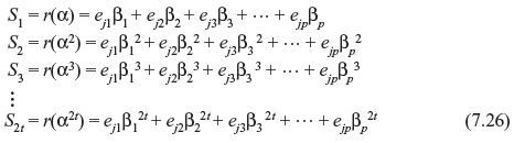
Figure 7.7 Encoding Scheme for Nonbinary BCH Code

The syndrome components S_i can also be computed by dividing r(x) by x + αⁱ, which results in the equality

 

 

The remainder b_i is constant in GF(2^m). Substituting αⁱ in both sides of Eq. (7.27), we obtain S_i = b_i.

The error location polynomial is computed by iterative method, where

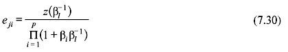
The error values can be determined by following computation. Let

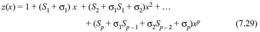
For i ≠ l, the error values at location β_l = α^jl is expressed as follows:

Example 7.4: Consider a triple-error-correcting Reed–Solomon code with symbols from GF(2⁴). The generator polynomial of this code is

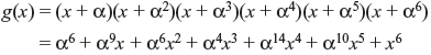
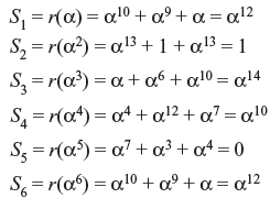
Let all-zero transmitted vector be received as r = (000α⁷00α³00000α⁴00). Therefore, the received polynomial r(x) = α⁷x³ + α³x⁶ + α⁴x¹². The syndrome components are calculated using Table 7.4 as follows:

To find the error location polynomial σ(x), iterative process is used, steps of which is tabulated in Table 7.6. The error location polynomial thus is found to be σ(x) = 1 + α⁷x + α⁴x³ + α⁵x³. Substituting 1, α, α², ..., α¹⁴ in σ(x), we find α³, α⁹, and α¹² are the roots and hence the error locations are reciprocal of them as α¹², α⁶, and α³. Now substituting the syndrome components in Eq. (7.29), we obtain that z(x) = 1 + α²x + x² + α⁶x³. Using the error value relation as in Eq. (7.30), we obtain e₃ = α⁷, e₆ = α³, and e₁₂ = α⁴. Thus, the error pattern is e(x) = α⁷x³ + α³x⁶ + α⁴x¹². This is exactly similar to the error location as assumed. Decoding is complete by addition of received vector and error vector, i.e., r(x) + e(x) which is the desired data.

 

Table 7.6 Computation of Error Location Polynomial

Reed–Solomon codes are very effective for correction of multiple burst errors.

7.9  WEIGHT DISTRIBUTION

The minimum distance of a linear code is the smallest weight of any nonzero code word, and is important because it directly affects the number of errors the code can correct. However, the minimum distance says nothing about the weights of other code words in the code; and hence, it is necessary to look at the weight distribution of the entire code. It turns out that the weight distribution of many types of codes, including Hamming and BCH codes, is asymptotically normal (i.e., it approaches the normal distribution for large codes of a given variety). If A_i is the number of code vectors of weight i in (n, k) linear code C, the numbers A₁, A₂, ., A_n are called the weight distribution of C. If C is used only for error detection on a binary symmetric channel (BSC), the probability of undetected errors can be computed from the weight distribution of C. Since an undetected error occurs only when the error pattern is identical to nonzero code vector of C, the probability of undetected error P(E) may be expressed as follows:

where p is the transition probability of the BSC. If the minimum distance of C is d_min, then A₁ to A_{dmin – 1} are zero. It has been observed that the probability of undetected error P(E) for a double-error-correcting BCH code of length 2^m – 1 has the upper bound of 2^–2m for p ≤ ½, where 2m is the number of parity digits of the code.

For t-error-correcting primitive BCH of length 2^m – 1 with mt number of parity-check digits, where m is greater than certain constant m₀(t), it has been observed that the weight distribution satisfies the following equalities:

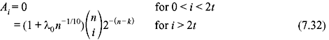
where n = 2^m – 1 and λ₀ is the upper bounded by a constant. From Eqs. (7.31) and (7.32), we obtain the expression for probability of undetected error P(E).

For ε = (2t + 1)/n and p < ε, the summation term of Eq. (7.33)

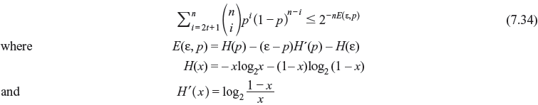
Therefore, for p < ε, the upper bound of P(E) is given as follows:

Similarly, for p > ε, since 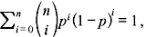we have the upper bound of P(E) as follows:

It may be noticed that probability of undetected error reduces exponentially with number of parity-check digits, n – k. Therefore, incorporation of sufficiently large number of parity digits results in reduction of probability of undetected errors. For nonbinary case, the weight distribution of t-error-correcting Reed–Solomon codes of length q – 1 with symbols from GF(q) is as follows:

7.10  SOLVED PROBLEMS

Problem 7.1: Find the generator polynomial of a triple-error-correcting BCH code with block length n = 31 over GF(2⁵).

Solution:

 

Block length:	n = 2m – 1 = 31, m = 5
Error-correction capability	t = 3
Number of parity-check digits:	n – k ≤ mt = 5 × 3 = 15
Minimum distance:	dmin ≥ 2t + 1 = 7

The minimal polynomials have the degree of less than or equal to 5 and they divide x²⁵ + x or x³² + x. Triple-error-correcting BCH code of length 31 contains the lowest degree polynomial with the roots as α, α², α³, ..., α⁶. The generator polynomial g(x) may be expressed as

 

 

As the degree of each polynomial is 5, the degree of g(x) is at most 15. From Table 7.3, the minimal polynomials are

Therefore,

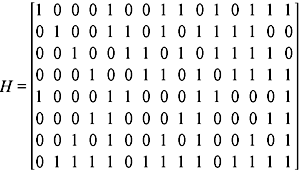
Problem 7.2: Find the parity-check matrix of a double-error-correcting (15, 4) BCH code.

Solution: For double-error-correcting (15, 4) BCH code the generator polynomial is Φ₁(x) = 1 + x + x⁴ whose primitive element is α.

Then the parity-check matrix may be written as follows:

From the characteristics of primitive elements, we have α¹⁵ = α³⁰ = 1, α¹⁸ = α³³ = α³, α²¹ = α³⁶ = α⁶, α²⁴ = α³⁹ = α⁹, and α⁴² = α¹². Due to conjugate elements of α, the Eq. (7.4) is reduced to

Using Table 7.4, the equivalent polynomial and its 4-tuple representation we obtain the following parity-check matrix.

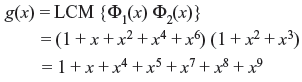
Problem 7.3: Construct a double-error-correcting BCH code over GF(2³).

Solution:

Double-error-correction code may be generated by the generator polynomial

Problem 7.4: Construct the (15, 7) double-error-correcting BCH code and code word is C(x) = 1 + x⁴ + x⁶ + x⁷ + x⁸. Determine the outcome of a decoder when C(x) incurs the error pattern e(x) = 1 + x² + x⁷.

Solution:

The generated code is (15, 7) and the minimal polynomials over GF(2⁴)

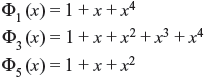
Double-error-correction BCH code is generated by the generator polynomial

For the code word C(x) = 1 + x⁴ + x⁶ + x⁷ + x⁸ incurring error as e(x) = 1 + x² + x⁷, the received vector r(x) = C(x) + e(x), i.e.,

Therefore, the decoder output is x² + x⁴ + x⁶ + x⁸.

Problem 7.5: Consider double-error-correcting code over GF(2⁶) of the order of n = 21, where the element β = α³. Find the polynomial of minimum degree that has the roots β, β², β³, and β⁴. Which BCH code may be developed?

Solution: The elements β, β², and β⁴ have the same polynomial, Φ₁(x) = 1 + x + x² + x⁴ + x⁶.

The element β³ has the minimal polynomial Φ₂(x) = 1 + x² + x³.

Therefore, the generator polynomial of minimum degree is

The above polynomial divides 1 + x²¹. As t = 2 and m = 6, k = n – mt = 9. Therefore, a (21, 9) BCH code may be generated.

Problem 7.6: Consider a triple-error-correcting binary BCH (15, 5) code with generator polynomial g(x) = 1 + x + x² + x⁴ + x⁵ + x⁸ + x¹⁰. The received polynomial is r(x) = x³ + x⁵. Find the code word.

Solution: For t-error-correcting BCH code, the error location can be obtained by solving the following relation of syndrome matrix form.

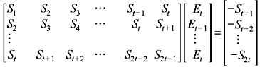
The syndromes are computed by substituting αⁱ in the received polynomial r(x) = x³ + x⁵ for 1 ≤ i ≤ 2t, where t is error-correction capability. Using the Table 7.4, as t = 3, they are as follows:

The syndrome matrix is obtained as below (number or rows and columns are limited to t = 3)

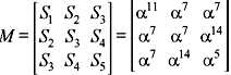
Det [M] = 0, which implies that there are fewer than three errors are present in the received vector. Next matrix has generated for t ≤ 2, which given as

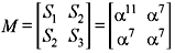
where Det [M] ≠ 0. Therefore, two errors have been occurred. Error location may be obtained from following matrix computation.

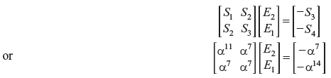
Solving the above equation, we obtain E₂ = α⁸ and E₁ = α¹¹. Thus, error polynomial is e(x) = 1 + α¹¹x + α⁸x². This may be written as e(x) = (1 + α³x) (1 + α⁵x). Therefore, the error locations are at α³ and α⁵ or e(x) = x³ + x⁵. The code word may be computed as c(x) = r(x) + e(x) = x³ + x⁵ + x³ + x⁵ = 0. This means all-zero code word was sent.

MULTIPLE CHOICE QUESTIONS

1. For m = 4, what is the block length of the BCH code?
   1. 16 
   2. 15 
   3. 16 
   4. none of these

   Ans. (b)

2. What is the error-correction capability of a (15, 5) BCH code over GF(2⁴)?
   1. 1 
   2. 2 
   3. 3 
   4. 4

   Ans. (c)

3. If t is the error-correction capability of a BCH code what is the minimum distance of the code?
   1. 2t 
   2. 2t + 1 
   3. 2t – 1 
   4. none of these

   Ans. (b)

4. For BCH code, if the received vector and computed error vector are r(x) and e(x), then the error-free code vector can be calculated as
   1. r(x) · e(x) 
   2. r(x)/e(x) 
   3. r(x) + e(x) 
   4. none of these

   Ans. (c)

5. For (15, 5) BCH code, if the roots of error location polynomial α(x) are α², α⁷, and α⁹, then error polynomial e(x) is
   1. x² + x⁷ + x⁹
   2. x⁶ + x⁸ + x¹³
   3. x⁷ + x¹² + x¹⁴
   4. none of these

   Ans. (b)

6. For a BCH code, if the minimal polynomials are Φ_i(x) (1 ≤ i ≤ 7), the generator polynomial g(x) of triple error correction is
   1. LCM{Ф₁(x)Ф₂(x)}
   2. LCM{Ф₁(x)Ф₃(x)}
   3. LCM{Ф₁(x)Ф₂(x)Ф₃(x)}
   4. LCM{Ф₁(x)Ф₃(x)Ф₅(x)}

   Ans. (d)

7. A BCH code over GF(2⁶) can produce the code maximum error capability of
   1. 6
   2. 8
   3. 10
   4. 12

   Ans. (c)

8. A (63, 15) BCH code over GF(2⁶) can produce the code maximum error capability of
   1. 6
   2. 8
   3. 10
   4. 12

   Ans. (b)

REVIEW QUESTIONS

1. Determine all generator polynomials for block length 31.
2. Decode the BCH code of block length 3, if the received polynomials are r₁(x) = x⁷ + x³⁰ and r₂(x) = 1 + x¹⁷ + x²⁸.
3. Prove that the syndrome components related as S_2i = S_i².
4. If a BCH code of length n = 2^m – 1 has t-error-correcting capability and 2t + 1 is a factor of n, prove that the minimum distance of the code is exactly 2t + 1.
5. Using p(x) = 1 + x² + x⁵ devise a circuit that is capable of multiplying two elements in GF(2⁵).
6. Devise a syndrome computation circuit for a double-error-correcting (31, 21) BCH code.
7. A t-error-correcting Reed–Solomon code of GF(2^m) has the generator polynomial g(x) = (x + α)(x + α²)(x + α³) … (x + α^2t).

   Show that it has error-correction capability of 2t – 1, where α is the primitive element.

8. Device a syndrome computation circuit for single-error Reed–Solomon code of block length 15 from field of GF(2⁴).
9. Find the generator polynomial of double-error-correcting Reed–Solomon code of block length 15 over GF(2⁴). Decode the received polynomial r(x) = αx³ + α¹¹x⁷.