Table of Contents for

Information Theory, Coding and Cryptography

Chapter 4

Coding Theory

4.1  INTRODUCTION

Demand for efficient and reliable data transmission and storage systems is gaining more and more importance in recent years. With the emergence of new and sophisticated electronic gadgets as well as that of large scale, high-speed data networks demand is accelerated. In this sphere, a major concern of the designer is the control of errors so that reliable reproduction of data is obtained. The emergence of coding theory dates back to 1948, when Shannon in his landmark paper ‘A mathematical theory of communication’ demonstrated that, by proper encoding of the information, errors induced by a noisy channel or storage medium can be reduced to any desired level. Since then, a lot of work has been done for devising efficient encoding and decoding methods for error control in a noisy environment.

A typical transmission (or storage) system is illustrated schematically in Figure 4.1. In fact, transmission and digital data storage system have much in common. The information source shown can be a machine or a person. The source output can be a continuous waveform (i.e., analogue in nature) or a sequence of discrete symbols (i.e., digital in nature). Source encoder transforms the source output into a sequence of binary digits (bits) known as the information sequence u. If the source is a continuous one, then analogue-to-digital conversion process is also involved. The process of source coding is already discussed in detail in Chapter 3. The channel encoder transforms the information sequence u into a discrete encoded sequence v known as a code word. Generally v is also a binary sequence. But in some instances non-binary code words are also used.

 

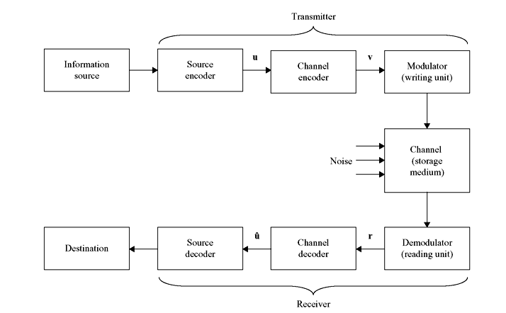
Figure 4.1 Schematic Diagram of a Data Transmission or Storage System

Since discrete symbols are not suitable for transmission over a physical channel or recording on a digital storage medium, usually the modulator (or writing unit) transforms each output symbol of the channel encoder into a waveform of duration t seconds. These waveforms enter the channel (or storage medium) and are then corrupted by noise. Then the demodulator (or reading unit) processes each received waveform of duration t and produces an output that can be discrete (quantized) or continuous (unquantized). The sequence of demodulator outputs corresponding to the encoded sequence v is known as the received sequence r.

Then the channel decoder transforms the received sequence r into a binary sequence û known as the estimated sequence. Ideally û should be the replica of u, though the noise can cause some decoding errors. The source decoder transforms û into an estimate of the source output and delivers this estimate to the destination. If the source is continuous, it involves digital-to-analogue conversion.

4.2  TYPES OF CODES

There are two different types of codes commonly used—block codes and convolution codes. A block code is a set of words that has a well-defined mathematical property or structure, where each word is a sequence of a fixed number of bits. Encoder for a block code divides the information sequence into message blocks of k information bits each. A message block is represented by the binary k-tuple u = (u₁, u₂, u₃, ..., u_k) known as the message. Hence, there are totally 2^k different possible messages. The encoder will add some parity bits or check bits to the message bits and transform each message u independently into an n-tuple v = (v₁, v₂, v₃, ..., v_n) of discrete symbols. These are called code words. Thus, corresponding to 2^k different possible messages, there are 2^k different possible code words at the encoder output. This set of 2^k code words of length n is known as (n, k) block code.

The position of the parity bits within a code word is arbitrary. They can be dispersed within the message bits or kept together and placed on either side of the message bits. A code word whose message bits are kept together is said to be in systematic form, otherwise the code word is referred to as non-systematic. A block code whose code words are systematic is referred to as a systematic code. Here the n-symbol output code word depends only on the corresponding k-bit input message. Thus, the encoder is memoryless and hence can be implemented with a combinational logic circuit. Block codes will be discussed in detail in Chapters 5–7.

4.2.1  Code Rate

The ratio R = k/n is called the code rate. This can be interpreted as the number of information bits entering the encoder per transmitted symbol. Thus, this is a measure of the redundancy within the block code. For a binary code to have a different code word assigned to each message, k ≤ n or R ≤ 1. When k < n, (n – k) redundant bits can be added to each message to form a code word. These redundant bits provide the code the power to combat with channel noise. For a fixed number of message bits, the code rate tends to 0 as the number of redundant bits increases. On the contrary, for the case of no coding there are no parity bits and hence n = k and the code rate R = 1. Thus, we see that the code rate is bounded by 0 ≤ R ≤ 1.

Encoder for a convolution code also accepts k-bit blocks of message sequence u and produces an encoded sequence v of n-symbol blocks. However, each encoded block depends on the corresponding k-bit message block, as well as on the previous m message blocks. Thus, the encoder has a memory order of m. This set of encoded sequences produced by a k-input, n-output encoder of memory order m is known as (n, k, m) convolution code. Since the encoder has memory, it is implemented with sequential logic circuit. Here also the ratio R = k/n is called the code rate. In a binary convolution code, redundant bits can be added when k < n or R < 1. Generally k and n are small integers and more redundancy is added by increasing m while maintaining k and n and hence code rate R fixed. Convolution code is discussed in detail in Chapter 8.

4.3  TYPES OF ERRORS

In general, errors occurring in channels can be categorized into two types—random error and burst error. On memoryless channels, noise affects each transmitted symbol independently. Thus, transmission errors occur randomly in the received sequence. Memoryless channels are thus known as random-error channels, e.g., deep-space channels, satellite channels, etc. Codes used for correcting random errors are called random-error-correcting codes.

On the other hand, on channels with memory, noise is not independent for each transmission. As a consequence, a transmission error occurs in clusters or bursts in these channels called burst-error channels, e.g., radio channels, wire and cable transmission, etc. Codes devised for correcting burst errors are called burst-error-correcting codes. Finally it is to mention that some channels contain a combination of both random and burst errors. These are known as compound channels and the codes used for correcting errors on these channels are called burst-and-random-error-correcting codes.

4.4  ERROR CONTROL STRATEGIES

Transmission or storage system can be either a one-way system, where the transmission or recording is strictly in one direction, from transmitter to receiver, or a two-way system, i.e., information can be sent in both directions and the transmitter also acts as a receiver (a transceiver) and vice versa.

For a one-way system, error control is accomplished by using forward error correction (FEC). Here error-correcting codes automatically correct errors detected at the receiver. In fact most of the coded systems in use today use some form of FEC, even if the channel is not strictly one way. Examples of such one-way communication are broadcast systems, deep space communication systems, etc.

On the other hand, error control for a two-way system can be accomplished by using automatic repeat request (ARQ). In these systems, whenever an error is detected at the receiver, a request is sent for the transmitter to repeat the message, and this will continue until the total message is received correctly. Examples of two-way communication are some satellite communication channels, telephone channels, etc.

ARQ systems are of two types: continuous ARQ and stop-and-wait ARQ. With the continuous ARQ, the transmitter sends code words to the receiver continuously and receives acknowledgements continuously. If a negative acknowledgement (NAK) is received, the transmitter begins a retransmission. It backs up to the erroneous code word and resends that word plus the following words. This is known as go-back-N ARQ. Alternatively, the transmitter can follow selective-repeat ARQ, where only those code words which are acknowledged negatively are resent. Selective-repeat ARQ requires more logic and buffering than go-back-N ARQ, but at the same time is more efficient.

With the stop-and-wait ARQ, the transmitter sends a code word to the receiver and waits for a positive acknowledgement (ACK) or a NAK from the receiver. If no errors are detected, i.e., ACK is received, the transmitter sends the next code word. Alternatively, if errors are detected and NAK is received, it resends the preceding code word.

Continuous ARQ is more efficient that stop-and-wait ARQ, but it is more expensive. In channels where the transmission rate is high but time taken to receive an acknowledgement is more, generally continuous ARQ is used, e.g., satellite communication system. On the other hand, in channels where the transmission rate is low compared to the time to receive an acknowledgement, stop-and-wait ARQ is used. Generally continuous ARQ is used on full duplex channels, whereas stop-and-wait ARQ is used on half duplex channels.

ARQ is advantageous over FEC, in the sense in the former only error is detected and in the later case error is detected as well as corrected. Since error detection requires much simple decoding circuit than error correction, implementation of ARQ is simpler compared to FEC. The disadvantage of ARQ is that when the channel error rate is high, retransmissions are required too often, and the rate at which newly generated messages are correctly received, i.e., the system throughput is lowered by ARQ. In such a situation, a combination of FEC for the frequent error patterns, together with ARQ for the less likely error patterns, is much efficient.

4.4.1  Throughput Efficiency of ARQ

In ARQ systems, the performance is usually measured using a parameter known as throughput efficiency. The throughput efficiency is defined as the ratio of the average number of information bits per second delivered to the user to the average number of bits per second that have been transmitted in the system. This throughput efficiency is obviously smaller than 100%. For example, using an error-detecting scheme with a code rate R = 0.97, an error-free transmission would then correspond to a throughput efficiency of 97%.

A. Stop-and-Wait ARQ   For error-free operation using the stop-and-wait ARQ technique, the utilization rate U_R of a link is defined as

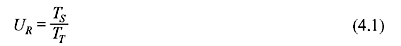
where T_s denotes the time required to transmit a single frame, and T_T is the overall time between transmission of two consecutive frames, including processing and ACK/NAK transmissions. The total time T_T can be expressed as follows:

 

 

In above equation, T_p denotes the propagation delay time, i.e., the time needed for a transmitted bit to reach the receiver; T_c is the processing delay time, i.e., the time required for either the sender or the receiver to perform the necessary processing and error checking, whereas T_s and T_a denote the transmission duration of a data frame and of an ACK/NAK frame, respectively.

Assuming the processing time T_c is negligible with respect to T_p and that the sizes of the ACK/NAK frames are very small, leading T_a to negligible value, then from the above equation we can write:

 

 

Defining the propagation delay ratio as α = T_p/T_s, then U_R can be written as follows:

The utilization rate expressed in Eq. (4.4) can be used to evaluate the throughput efficiency on a per-frame basis. Due to repetitions caused by transmission errors, the average utilization rate, or throughput efficiency, is defined as follows:

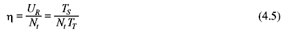
where N_t is the expected number of transmissions per frame.

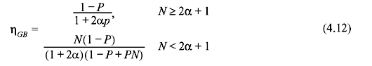
In this definition of the throughput efficiency [i.e., Eq. (4.5)], the coding rate of the error-detecting code, as well as the other overhead bits, is not taken into account. That is, the above equation represents the throughput efficiency on a per-frame performance basis. Some other definitions of the throughput deficiency can be related to the number of information bits actually delivered to the destination. In such a case, the new throughput efficiency is simply:

 

 

where ρ represents the fraction of all redundant and overhead bits in the frame.

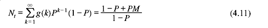
Assuming error-free transmissions of ACK and NAK frames, and assuming independence for each frame transmission, the probability of requiring exactly k attempts to successfully receive a given frame is P_k = P^{k – 1}(1 – P), k = 1, 2, 3, ..., where P is the frame error probability. The average number of transmissions N_t that are required before a frame is accepted by the receiver is then

Using Eqs. (4.4), (4.5), and (4.7) the throughput efficiency can thus be written as follows:

B. Continuous ARQ   For continuous ARQ schemes, the basic expression of the throughput efficiency shown in Eq. (4.8) must be used with the following assumptions: The transmission duration of a data frame is normalized to T_s = 1; the transmission time of an ACK/NAK frame, T_a, and the processing delay of any frame, T_c, are negligible. Since α = T_p/T_s and T_s = 1, the propagation delay T_p is equal to α. Assuming no transmission errors, the utilization rate of the transmission link for a continuous ARQ using a sliding window protocol of size N is given by:

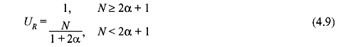
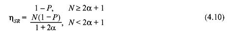
Selective-Repeat ARQ: For selective-repeat ARQ scheme, the expression for the throughput efficiency can be obtained by dividing Eq. (4.9) by yielding

Go-back-N ARQ: For the go-back-N ARQ scheme, each frame in error necessitates the retransmission of M frames (M ≤ N) rather than just one frame, where M depends on the roundtrip propagation delay and the frame size. Let g(k) denote the total number of transmitted frames corresponding to a particular frame being transmitted k times. Since each repetition involves M frames, we can write

 

 

Using the same approach as in Eq. (4.7), the average number of transmitted frames N_t to successfully transmit one frame can be expressed as follows:

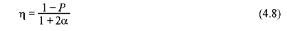
If N ≥ 2α + 1, the sender transmits continuously and, consequently, M is approximately equal to 2α + 1. In this case, in accordance with Eq. (4.11), N_t = (1 + 2αΡ)/(1 – P). Dividing Eq. (4.9) by N_t, the throughput efficiency becomes η = (1 – P)/(1 + 2αP).

If N < 2α + 1, then M = N and hence N_t = (1 – P + PN)/(1 – P). Dividing Eq. (4.9) again by N_t, we obtain U = N(1 – P)/(1 + 2α)(1 – P + PN).

Summarizing, the throughput efficiency of go-back-N ARQ is given by

4.5  MATHEMATICAL FUNDAMENTALS

To understand the coding theory, it is essential for the reader to have an elementary knowledge of the algebra involved in this. In this section we try to develop a general understanding of the coding algebra. Here, we basically approach in a descriptive way rather than becoming mathematically rigorous.

4.5.1  Modular Arithmetic

Modular arithmetic (sometimes called clock arithmetic) is a system of arithmetic of congruences, where numbers ‘wrap around’ after they reach a certain value, called the modulus. If two values x and y have the property that their difference (x – y) is integrally divisible by a value m (i.e., (x – y)/m is an integer), then x and y are said to be ‘congruent modulo m.’ The value m is called the modulus, and the statement ‘x is congruent to y (modulo m)’ is written mathematically as x ≡ y (mod m). On the contrary if (x – y) is not integrally divisible by m, then it is said that ‘x is not congruent to y (modulo m)’.

It is known that set of integers can be broken up into the following two classes:

• the even numbers (..., –6, –4, –2, 0, 2, 4, 6, ...)
• the odd numbers (..., –5, –3, –1, 1, 3, 5, ...).

Certain generalizations can be made about the arithmetic of numbers based on which of these two classes come from. For example, we know that the sum of two even numbers is even. The sum of an even number and an odd number is odd. The sum of two odd numbers is even. The product of two even numbers is even, etc.

Modular arithmetic lets us state these results quite precisely, and it also provides a convenient language for similar but slightly more complex statements. In the above example, our modulus is the number 2. The modulus can be thought of as the number of classes that we have broken the integers up into. It is also the difference between any two ‘consecutive’ numbers in a given class.

Now we represent each of our two classes by a single symbol. We assume number ‘0’ means ‘the class of all even numbers’ and number ‘1’ means ‘the class of all odd numbers’. There is no great reason why we have chosen 0 and 1; we could have chosen 2 and 1, or any other numbers, but 0 and 1 are the conventional choices.

The statement ‘the sum of two even numbers is even’ can be expressed by the following:

 

 

where the symbol ‘≡’ is not equality but congruence, and the ‘mod 2’ just signifies that modulus is 2. The above statement is read as ‘Zero plus zero is congruent to zero, modulo two’. The statement ‘the sum of an even number and an odd number is odd’ is represented by

 

 

Similarly ‘the sum of two odd numbers is even’ is written as:

 

 

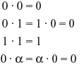
where the symbol ‘≡’ and ‘mod 2’ are very important. We have analogous statements for multiplication:

 

 

In a sense, we have created a number system with addition and multiplication but in which the only numbers that exist are 0 and 1. This number system is the system of integers modulo 2, and as a result of the afore-mentioned six properties, any arithmetic done in the integers translates to arithmetic done in the integers modulo 2. This means that if we take any equality involving addition and multiplication of integers, say

 

 

and reducing each integer modulo 2 (i.e., replacing each integer by its class ‘representative’ 0 or 1), we will obtain a valid congruence. The above equation reduces to

More useful applications of reduction modulo 2 are found in solving equations. Suppose we want to know which integers might solve the equation

 

 

Of course, we can solve for a only if we take into account whether a is even or odd, irrespective of other factors, by proceeding with the following. Reducing modulo 2 gives the congruence

 

 

or

 

 

so any integer a satisfying the equation 5a – 5 = 25 must be even.

Since any integer solution of an equation reduces to a solution modulo 2, it follows that if there is no solution modulo 2 then there is no solution in integers. For example, assume that a is an integer solution to

 

 

which reduces to

 

 

or 1 ≡ 0 mod 2. This is a contradiction because 0 and 1 are different numbers modulo 2 (no even number is an odd number, and vice versa). Therefore, the above congruence has no solution; hence, a is not an integer. This proves that the equation 2a – 1 = 14 has no integer solution.

Less trivially, consider the system of equations

 

 

Modulo 2: These equations reduce to

 

 

This says that b is both even and odd, which is a contradiction. Therefore, we know that the original system of equations has no integer solutions, and to prove this we didn’t even need to know anything about a.

As shown by the preceding examples, one of the powers of modular arithmetic is the ability to show, often very simply, that certain equations and systems of equations have no integer solutions. Without modular arithmetic, we would have to find all of the solutions and then see if any turned out to be integers.

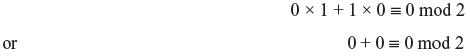
In Modulo 2, all of the even numbers are congruent to each other since the difference of any two even numbers is divisible by 2:

Also, every odd number is congruent to every other odd number modulo 2 since the difference of any two odd numbers is even:

Therefore, we can replace ‘0’ by any even number, and similarly ‘1’ by any odd number. For example, instead of writing 0 × 1 + 1 ×0 ≡ 0 mod 2, an equally valid statement is

 

 

Let’s now look at other values for the modulus m. For example, let m = 3. All multiples of 3 are congruent to each other modulo 3 since the difference of any two is divisible by 3. Similarly, all numbers of the form 3n + 1 are congruent to each other, and all numbers of the form 3n + 2 are congruent to each other.

 

 

However, when m = 1, the difference of any two integers is divisible by 1; hence, all integers are congruent to each other modulo 1:

 

 

For this reason, m = 1 is not very interesting, and reducing an equation modulo 1 doesn’t give any information about its solutions.

The modulus m = 12 comes up quite frequently in everyday life, and its application illustrates a good way to think about modular arithmetic—the ‘clock arithmetic’ analogy. If it is 5:00, what time will it be in 13 hours? Since 13 ≡ 1 mod 12, we simply add 1 to 5:

 

 

So the clock will read 6:00. Of course, we don’t need the formality of modular arithmetic in order to compute this, but when we do this kind of computation in our heads, this is really what we are doing.

With m = 12, there are only 12 numbers (‘hours’) we ever need to think about. We count them 1, 2, 3, ..., 10, 11, 12, 1, 2, ..., starting over after 12. The numbers 1, 2, ..., 12 represent the twelve equivalence classes modulo 12: Every integer is congruent to exactly one of the numbers 1, 2, ..., 12, just as the hour on the clock always reads exactly one of 1, 2, ..., 12. These classes are given by

 

 

as n ranges over the integers.

Of course, the minutes and seconds on a clock are also modular. In these cases the modulus is m = 60. If we think of the days of the week as labelled by the numbers 0, 1, 2, 3, 4, 5, 6, then the modulus is m = 7. The point is that we measure many things, both in mathematics and in real life, in periodicity, and this can usually be thought of as an application of modular arithmetic.

4.5.2  Sets

Normally we define a set as a ‘collection of objects’. But mathematically we want to define a set such that objects either belong to the set or do not belong to the set. There is no other state possible. Thus, a set with n objects is written as {s₁, s₂, s₃, ..., s_n}. The objects s₁, s₂, s₃, ..., s_n are the elements of the set. This set is a finite set as there is finite number of elements in the set. If a set is formed taking any m elements from the set of n elements, where m ≤ n, then the new set formed is known as a subset of the original set of n elements. Example of a finite set is set of octal digits {0, 1, 2, 3, 4, 5, 6, 7}. Similarly, a set of infinite number of elements is referred to as an infinite set. Example of such an infinite set is a set of all integers {0, ±1, ±2, ±3, ...}.

We hope the readers are familiar with the idea of different mathematical operations between sets, namely intersection and union of sets that give the set of common elements and set of all elements, respectively. However, here we are more interested in operations between elements within a set, rather than operations between sets. So now we introduce ‘higher’ mathematical structures known as group.

4.5.3  Groups

Let us consider a set of elements G. We define a binary operation * on G such that it is a rule that assigns to each pair of elements a and b a uniquely defined third element c = a * b in G. If such a binary operation is defined on G, we say that G is closed under *.

Let us consider an example, where G is the set of all integers and the binary operation on G is real multiplication ×. For any two integers i and j in G, i × j is a uniquely defined integer in G. Thus, the set of integers is closed under real multiplication. The binary operation * on G is said to be associative if, for any a, b and c in G,

 

 

We now introduce a very useful algebraic system called a group.

Definition 4.1: A set G on which a binary operation * is defined is called a group if the following conditions are satisfied:

1. The binary operation * is associative.
2. G contains an element e, called an identity element on G, such that, for any a in G,

    

   a * e = e* a = a        (4.14)

    

3. For any element a in G, there exists another element a', called an inverse of a in G, such that

    

   a * a' = a' * a = e         (4.15)

A group G is said to be commutative if its binary operation * satisfies the following condition: For any a and b in G,

 

 

We now state two important conditions of groups which are to be satisfied:

1. The inverse of a group element is unique.
2. The identity element in a group G is unique.

Under real addition the set of all integers is a commutative group. In this case, the integer 0 is the identity element and the integer –i is the inverse of integer i. The set of all rational numbers excluding zero is a commutative group under real multiplication. The integer 1 is the identity element with respect to real multiplication, and the rational number b/a is the multiplicative inverse of a/b. The group discussed above contains infinite number of elements. But groups with finite numbers of elements do exist, as we shall see in the next example.

Example 4.1: Show that the set of two integers G = {0,1} is a group under the binary operation ⊕ on G as follows:

Solution: The binary operation ⊕ shown in the problem is called modulo-2 addition. It follows from the definition of modulo-2 addition ⊕ that G is closed under ⊕ and ⊕ is commutative. We can easily check that ⊕ is also associative. The element 0 is the identity element. The inverse of 0 is itself and the inverse of 1 is also itself. Thus, the set G = {0,1} together with ⊕ is a commutative group.

Order of Group: The number of elements in a group is known as the order of the group. A group having finite number of elements is called a finite group. For any positive integer m, it is possible to construct a group of order m under a binary operation, which is very similar to real addition. We show it in the following example.

Example 4.2: Show that the set of integers G = {0,1,2,..., m –1} forms a group under modulo-m addition. Here m is a positive integer.

Solution: Let us define modulo-m addition by the binary operator [+] on G as follows: For any integers a and b in G,

 

 

where r is the remainder resulting from dividing (a + b) by m. By Euclid’s division algorithm, the remainder r is an integer between 0 and (m – 1) and is hence in G. Thus, G is closed under the binary operation [+], which is called modulo-m addition.

Now we prove that the set G = {0,1,2,...,m – 1}is a group under modulo-m addition.

First we see that 0 is the identity element. For 0 < a < m, a and (m – 1) are both in G. Since

 

 

It can be written from the definition of modulo-m addition that

 

 

Thus, a and (m – a) are inverses to each other with respect to [+]. The inverse of 0 is itself. Since, real addition is commutative, it follows from the definition of modulo-m addition that, for any a and b in G, a [+] b = b [+] a. Hence, modulo-m addition is commutative.

Now we show that modulo-m addition is associative. We have

 

 

Dividing (a + b + c) by m, we obtain

 

 

where q and r are the quotient and the remainder, respectively, and 0 ≤ r ≤ m. Now dividing (a + b) by m, we have

 

 

with 0 ≤ r₁ ≤ m. Thus, a [+]b = r₁. Dividing (r₁ + c) by m, we have

 

 

with 0 ≤ r₂ ≤ m. Thus, r₁ [+]c = r₂ and

 

 

Combining Eqs. (4.18) and (4.19), we have

 

 

This implies that r₂ is also the remainder when (a + b + c) is divided by m. Since the remainder resulting from dividing an integer by an integer is unique, we must have r₂ = r. As a result, we have

 

 

Similarly, it can be shown that,

 

 

Therefore, (a[+]b) [+]c = a[+] (b[+]c) and modulo-m addition is associative.

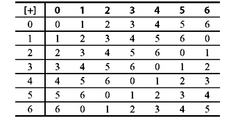
Thus, we prove that the set G = {0,1,2,...,m – 1} is a group under modulo-m addition. We shall call this group an additive group. For m = 2, we obtain the binary group given in Example 4.1. The additive group under modulo-7 addition is given in Table 4.1.

 

Table 4.1 Modulo-7 Addition

Finite groups with a binary operation similar to real multiplication can also be constructed.

Example 4.3: Let p be a prime (e.g., p = 2, 3, 5, 7, 11, 13, 17, ...). Show that the set of integers G = {1,2,3,4,..., p – 1} forms a group under modulo-p multiplication.

Solution: Let us define modulo-p multiplication by the binary operator [·] on G as follows: For any integers a and b in G,

 

 

where r is the remainder resulting from dividing (a · b) by p. We note that (a · b) is not divisible by p. Hence, 0 < r < p and r is an element in G. Thus, G is closed under the binary operation [·], which is called modulo-p multiplication. Now we will show that the set G = {1,2,3,..., p – 1} is a group under modulo-p multiplication.

It can be easily checked that modulo-p multiplication is commutative and associative. The identity element is 1. The only thing to be proved is that every element in G has an inverse. Let a be an element in G. Since a < p and p is a prime, a and p must be relatively prime. By Euclid’s theorem, it is well known that there exist two integers i and j such that

 

 

where i and p are relatively prime. Rearranging Eq. (4.24), we have

 

 

From Eq. (4.25), we can say that if (i · a) is divided by p, the remainder is 1. If 0 < i < p, then i is in G and it follows from Eq. (4.25) and the definition of modulo-p multiplication that

 

 

Hence, i is the inverse of a. On the contrary, if i is not contained in G, we divide i by p, and get

 

 

Since, i and p are relatively prime, the remainder r cannot be 0 and it must be between 1 and (p – 1). Hence, r is in G. Now, from Eqs. (4.25) and (4.26), we have

 

 

Therefore, r [·] a = a[·] r = 1 and r is the inverse of a. Thus, any element a in G has an inverse with respect to modulo-p multiplication. The group G = {1, 2, 3, ..., p – 1} under modulo-p multiplication is called a multiplicative group. For p = 2, we obtain a group G = {1} with only one element under modulo-2 multiplication.

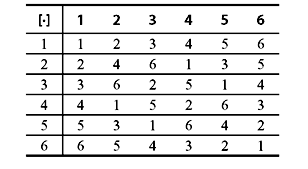
Note: If p is not a prime, the set G = {1, 2, 3, ..., p – 1} is not a group under modulo-p multiplication. The multiplicative group under modulo-7 multiplication is given in Table 4.4.

 

Table 4.2 Modulo-7 Multiplication

4.5.4  Fields

We now introduce another very important algebraic system called a field. We will use the concepts of group to describe the field. In a rough sense, field is a set of elements in which we can perform addition, subtraction, multiplication and division without leaving the set. Addition and multiplication must satisfy the commutative, associative, and distributive laws. Now we formally define a field as follows:

Definition 4.2: Let F be a set of elements in which two binary operations, addition ‘+’ and multiplication ‘·’, are defined. The set F along with the two binary operations (+) and (·) is a field if the following conditions are satisfied:

1. The set of nonzero elements in F is a commutative group under multiplication. The identity element with respect to multiplication is called the unit element or the multiplicative identity of F and is denoted by 1.
2. F is a commutative group under addition. The identity element with respect to addition is called the zero element or the additive identity of F and is denoted by 0.
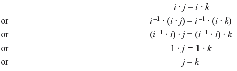
3. Multiplication is distributive over addition; i.e., for any three elements i, j and k in F,

    

   i · (j + k) = i · j + i · k

From the definition of field it can be said that a field consists of at least two elements, the multiplicative identity and the additive identity.

Order of Field: The number of elements in a field is known as the order of the field. A field having finite number of elements is called a finite field.

In a field, the additive inverse of an element i is denoted by –i, and the multiplicative inverse of i is denoted by i^–1, provided i ≠ 0. Thus, subtracting a field element j from another field element i is defined as adding the additive inverse –j of j to i. Similarly, if j is a nonzero element, dividing i by j is defined as multiplying i by the multiplicative inverse j^–1 of j. Some basic properties of fields are now derived from the definition of a field.

Property 1: For every element i in a field, i · 0 = 0 · i = 0.

Proof: We have

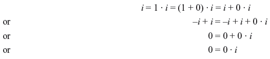
Similarly, we can prove that i · 0 = 0. Hence, we obtain i · 0 = 0 · i = 0.

Property 2: For any two nonzero elements i and j in a field, i · j ≠ 0.

Proof: Since nonzero elements of a field are closed under multiplication, the property is proved.

Property 3: For any two elements i and j in a field, i · j = 0 and i ≠ 0 imply that j = 0.

Proof: This is a direct consequence of Property 2.

Property 4: For any two elements i and j in a field, –(i · j) = (–i) · j = i · (–j)

Proof: We have

 

 

Hence, (–i) · j should be the additive inverse of i · j and –(i · j) = (–i) · j.

Similarly, we can prove that –(i · j) = i · (–j).

Property 5: For i ≠ 0, i · j = i · k implies that j = k.

Proof: Since i is a nonzero element in the field, it should have a multiplicative inverse i^–1.

Now

The set of real numbers is a field under real addition and multiplication. This field has infinite number of elements. If the number of elements is finite then the field is called finite field.

Example 4.4: Construct a finite field having only two elements {0,1}.

Solution: Let us consider the set {0,1} with modulo-2 addition and multiplication shown in Tables 4.3 and 4.4.

 

Table 4.3 Modulo-2 Addition

+	0	1
0	0	1
1	1	0

 

Table 4.4 Modulo-2 Multiplication

+	0	1
0	0	0
1	0	1

We have already shown that {0,1} is a commutative group under modulo-2 addition in Example 4.1. Also in Example 4.3 we have shown that {1} is a group under modulo-2 multiplication. We can easily check that modulo-2 multiplication is distributive over modulo-2 addition by simply computing i · (j + k) and i · j + i · k for eight possible combinations of i, j and k (i = 1 or 0, j = 1 or 0 and k = 1 or 0). Thus, the set {0,1} is a field of two elements under modulo-2 addition and modulo-2 multiplication.

The field discussed in Example 4.4 is called binary field and is denoted by GF(2). This field plays a very important role in coding theory.

Let us consider that p is a prime number. The set of integers {0, 1, 2, ..., p – 1} forms a commutative group under modulo-p addition (as shown in Example 4.2). We have also shown in Example 4.3 that the nonzero elements {1, 2, ..., p – 1} forms a commutative group under modulo-p multiplication. We can show that modulo-p multiplication is distributive over modulo-p addition. Hence, the set {0, 1, 2, ..., p – 1} is a field under modulo-p addition and multiplication. Since the field is constructed from prime p, this field is known as a prime field and is denoted as GF(p).

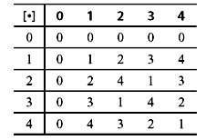
The set of integers {0, 1, 2, 3, 4} is a field of five elements. It is denoted by GF(5), under modulo-5 addition and multiplication. Addition table can also be used for subtraction. Say for example, if we want to subtract 4 from 2, first we should find out the additive inverse of 4 from Table 4.5, which is 1. Then add 1 to 2 to obtain the result 3 [i.e., 2 – 4 = 2 + (– 4) = 2 + 1 = 3]. Similarly in order to perform division, we can use the multiplication table. Suppose that we divide 4 by 3. The multiplicative inverse of 3 is first calculated, which is 2. Then we multiply 4 by 2 to obtain the result 3 [i.e., 4 ÷ 3 = 4 × (3^–1) = 4 × 2 = 3]. Thus, we see that, in a finite field, addition, subtraction, multiplication and division can be carried out in a similar fashion to ordinary arithmetic. Modulo-5 addition and multiplication are shown in Tables 4.5 and 4.6, respectively.

 

Table 4.5 Modulo-5 Addition

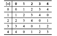
Table 4.6 Modulo-5 Multiplication

Thus, we can conclude that, for any prime p, there exists a finite field of p elements. Actually for any positive integer n, it is possible to extend the prime field GF(p) to a field of pⁿ elements. This is called an extension field of GF(p) and is denoted as GF(pⁿ). It can be proved that the order of any finite field is a power of a prime. Finite fields are also known as Galois fields (pronounced as Galva). Finite field arithmetic is very similar to ordinary arithmetic and hence most of the rules of ordinary arithmetic apply to finite field arithmetic.

Characteristic of Field: Let us consider a finite field of q elements, GF(q). We form the following sequence of sums of the unit element 1 in GF (q):

As the field is closed under addition, these sums should all be the elements of the field. Again since the field is finite, all these sums cannot be distinct. Thus, the sequence of sums should repeat itself at some point of time. Hence, we can say that there exist two positive integers m and n such that m > n and

This shows that Thus, there must exist a smallest positive integer λ such that This integer λ is called the characteristic of the field GF(q). For example, the characteristic of the binary field GF(2) is 2, since 1 + 1 = 0.

Now we state three relevant theorems. The proofs of these theorems are out of the scope of the current text.

Theorem 4.1: Let b be a nonzero element of a finite field GF(q). Then b^{q – 1} = 1.

Theorem 4.2: Let b be a nonzero element of a finite field GF(q). Let n be the order of b. Then n divides (q – 1).

Theorem 4.3: The characteristic λ of a finite field is prime.

Primitive Element: In a finite field GF(q), a nonzero element b is called primitive if the order of b is (q – 1). Thus, the powers of a primitive element generate all the nonzero elements of GF(q). In fact, every finite field has a primitive element.

Let us consider the prime field GF(5) illustrated in Tables 4.5 and 4.6. The characteristic of this field is 5. If we take the powers of the integer 3 in GF(5) using the multiplication table, we obtain 3¹ = 3, 3² = 3 × 3 = 4, 3³ = 3 × 3² = 2, 3⁴ = 3 × 3³ = 1.

Hence, the order of the integer 3 is 4 and the integer 3 is a primitive element of GF(5).

Extension Field: A field K is said to be an extension field, denoted by K/F, of a field F if F is a subfield of K. For example, the complex numbers are an extension field of the real numbers, and the real numbers are an extension field of the rational numbers.

The extension field degree (or relative degree, or index) of an extension field K/F, denoted by [K : F], is the dimension of K as a vector space over F, i.e., [K : F] = dim_FK.

Splitting Field: The extension field K of a field F is called a splitting field for the polynomial f (x) ∊ F[x] if f(x) factors completely into linear factors in K[x] and f(x) does not factor completely into linear factors over any proper subfield of K containing F. For example, the field extension is the splitting field for x² + 3 since it is the smallest field containing its roots, and Note that it is also the splitting field for x³ + 1.

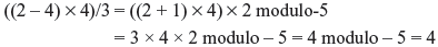
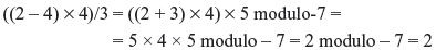
Example 4.5: Evaluate ((2 – 4) × 4)/3 over the prime field modulo-m when (a) m = 7 and (b) m = 5.

Solution:

1. In the prime field modulo-7 the additive inverse of 4 is 3 and the multiplicative inverse of 3 is 5.

   Thus,

   
2. On the other hand, in prime field modulo-5 the additive inverse of 4 is 1 and the multiplicative inverse of 3 is 2. Thus,
   

4.5.5  Arithmetic of Binary Field

Though codes with symbols from any Galois field GF(q), where q is either a prime p or a power of p, can be constructed, we are mainly concerned with binary codes with symbols from the binary field GF(2) or its extension GF(2ⁿ). So we will discuss arithmetic over the binary field GF(2) in detail.

In binary arithmetic, we use modulo-2 addition and multiplication, which we have already illustrated in Tables 4.3 and 4.4, respectively. The only difference of modulo-2 arithmetic with ordinary arithmetic lies in the fact that in modulo-2 arithmetic we consider 1 + 1 = 2 = 0. Hence, we can write

 

 

Thus, in binary arithmetic, subtraction is equivalent to addition.

We now consider a polynomial f(x) with one variable x and with coefficients from GF(2). ‘A polynomial with coefficients from GF(2)’ is also called as ‘a polynomial over GF(2)’. Let us consider:

 

 

where f_i = 0 or 1, for 0 ≤ i ≤ m. The degree of a polynomial is the largest power of x with a nonzero coefficient. For example in the above polynomial if f_m = 1, then the degree f(x) is m. On the other hand, if f_m = 0, then the degree f(x) is less than m.

Here there is only one polynomial of degree zero, namely

 

 

Again there are two polynomials of degree 1:

 

 

Similarly, we see that there are four polynomials over GF(2) with degree 2:

Thus, in general, there are 2^m polynomials over GF(2) with degree m.

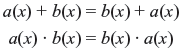
Polynomials over GF(2) can be added or subtracted, multiplied and divided in the usual way. We can also verify that the polynomials over GF(2) satisfy the following conditions:

1. Associative:
   
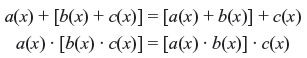
2. Commutative:
   
3. Distributive:
   

where a(x), b(x), and c(x) are three polynomials over GF(2). Now if s(x) is another nonzero polynomial over GF(2), then while dividing f(x) by s(x) we obtain a unique pair of polynomials over GF(2) – q(x), called the quotient, and r(x), called the remainder. Thus, we can write:

 

 

By Euclid’s division algorithm, the degree of r(x) is less than that of s(x). If the remainder r(x) is idential to zero, we say that f(x) is divisible by s(x) and s(x) is a factor of f(x).

For real numbers, if a is a root of a polynomial f(x) [i.e., f(a) = 0], we say that f(x) is divisible by x – a. This fact follows from Euclid’s division algorithm. This is still true for f(x) over GF(2). For example, let f(x) = 1 + x + x³ + x⁵. Substituting x = 1, we obtain

 

 

Thus, f(x) has 1 as a root and it can be verified that f(x) is divisible by (x + 1).

For a polynomial f(x) over GF(2), if it has an even number of terms, it is divisible by (x + 1). A polynomial p(x) over GF(2) of degree n is irreducible over GF(2) if p(x) is not divisible by any polynomial over GF(2) of degree less than n but greater than zero. For example, among the four polynomials of degree 2 over GF(2), three polynomials x², x² + 1 and x² + x are not irreducible since they are either divisible by x or x + 1. But x² + x + 1 does not have either ‘0’ or ‘1’ as a root and hence is not divisible by any polynomial of degree 1. Thus, x² + x + 1 is an irreducible polynomial of degree 2. Similarly it can be verified that x³ + x + 1, x⁴ + x + 1, and x⁵ + x + 1 are irreducible polynomials of degree 3, 4, and 5, respectively. It is true that for any n ≥ 1, there exists an irreducible polynomial of degree n. We state here a condition regarding irreducible polynomials over GF(2).

Any irreducible polynomial over GF(2) of degree n divides x^{2n – 1} + 1.

Eisenstein’s Irreducibility Criterion: Eisenstein’s irreducibility criterion is a sufficient condition assuring that an integer polynomial p(x) is irreducible in the polynomial ring Q(x). The polynomial p(x) = a_nxⁿ + a_{n –1}x^{n – 1} + ... + a₁x + a₀, where a_i ∈ Z for all i = 0, 1, ..., n and a_n ≠ 0 [which means that the degree of p(x) is n], is irreducible if some prime number p divides all coefficients a₀, ..., a_{n – 1}, but not the leading coefficient a_n, and, moreover, p² does not divide the constant term a₀.

This is only a sufficient, and by no means a necessary, condition. For example, the polynomial x² + 1 is irreducible, but does not fulfil the above property, since no prime number divides 1. However, substituting x + 1 for x produces the polynomial x² + 2x + 2, which does fulfil the Eisenstein criterion (with p = 2) and shows the polynomial is irreducible.

Primitive Polynomial: An irreducible polynomial p(x) of degree n is called primitive polynomial if the smallest positive integer m for which p(x) divides x^m + 1 is m = 2ⁿ – 1.

We can check that p(x) = x³ + x + 1 divides x⁷ + 1 but does not divide any x^m + 1 for 1 ≤ m ≤ 7. Hence, x³ + x + 1 is a primitive polynomial. It is not easy to recognize a primitive polynomial. For a given n, there can be more than one primitive polynomial of degree n. We list some primitive polynomials in Table 4.7. Here we list only one primitive polynomial with the smallest number of terms of each degree n. We now derive an useful property of polynomials over GF(2).

 

Table 4.7 Primitive Polynomials

n	Polynomial
3	x3 + x + 1
4	x4 + x + 1
5	x5 + x2 + 1
6	x6 + x + 1
7	x7 + x3 + 1
8	x8 + x4 + x3 + x2 + 1
9	x9 + x4 + 1
10	x10 + x3 +1
11	x11 + x2 + 1
12	x12 + x6 + x4 + x +1

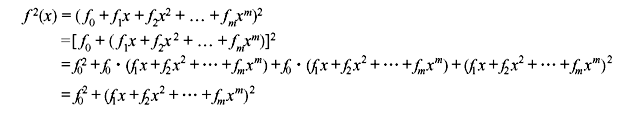
Similarly expanding the equation above repeatedly, we eventually obtain

As f_i = 0 or 1, f_i² = f_i . Thus, we have

It follows from (4.32) that, for any l ≥ 0,

 

4.5.6  Roots of Equations

In this section we shall discuss finite fields constructed from roots of equations. We will see that this is the basis of cyclic codes where all code word polynomials c(x) have the generator polynomial g(x) as a factor. We consider an algebraic equation of the form

where a₀ ≠ 0. We now consider that the coefficients of Eq. (4.34) are binary. The simplest algebraic equation is the equation of first degree which may be obtained by setting m = 1, and is written as follows:

 

 

There exists one root x = –a₀/a₁. The second degree (quadratic) equation is expressed as

 

 

This equation has two roots and is given by the well-known formula for solving quadratic equations

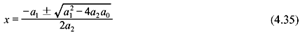
The roots of equations of third and fourth degrees can be similarly obtained algebraically, with three and four roots, respectively. However, it has been established that it is not possible to solve the fifth-degree equation using a finite number of algebraic operations. The same is true for equations of degree greater than five also. This does not necessarily mean that roots for fifth and higher degree equations do not exist, rather it can be stated that expressions for giving the roots do not exist. A fifth-degree equation will have five roots. Likewise an equation of degree m will have m roots. However, in some cases there is a slight problem regarding the nature of the roots. For example, in the quadratic equation a₂x² + a₁x + a₀ = 0, if we substitute a₂ = a₀ = 1 and a₁ = 0, we have

 

 

In this equation it is not possible to obtain two real numbers. Hence, the only way to obtain two roots for Eq. (4.36) is by defining a new imaginary number j (j here should not be confused with j in Section 4.5, where j was an element of the field), which satisfies

 

 

The number j can be combined with two real numbers p and q to give the complex number p + jq. Addition and multiplication over the set of all complex numbers obey the rules described in Sec. 4.5 for a set of elements to form a field. The resulting field is known as the complex field. Due to the existence of complex fields, all equations of degree m have m roots. The roots of Eq. (4.34) are of the form p + jq with real roots having q = 0.

Complex roots, of an equation with real coefficients, always occur in pairs known as complex conjugates. Thus, an equation can never have an odd number of complex roots, since that requires a complex root to exist without its conjugate. For example we can say that in an equation of degree three, either all the roots are real, or one of them is real while the other two are complex conjugates.

Complex field includes all the real numbers as they can be considered as field elements with q = 0. Basically the real field is referred to as the base field and the complex field as an extension field. In Eq. (4.34), the coefficients belong to the base field (i.e., the real field) whereas the roots belong to the extension field (i.e., the complex field). The occurrence of complex roots as conjugate pairs is necessary for the coefficients to lie in the real field.

Now we consider roots of equations of the form p(x) = 0, where p(x) is a polynomial with binary coefficients. Let us take an example

 

 

Since x can have a value of 0 or 1, we can substitute 0 and 1 directly into Eq. (4.38) to see whether 0 or 1 or both are roots. Substituting x = 0 or x = 1 into Eq. (4.38) gives 1, and so we have a binary polynomial without any binary roots. This is similar to the previous situation where we considered a real quadratic equation without any real roots. So the complex term j was introduced to tackle the problem. Similarly, here we define a new term such that it becomes a root of the polynomial of interest. Instead of using j to denote a root of Eq. (4.38), it is conventional to use α to represent the newly defined root. Substituting x = α into Eq. (4.38) gives

 

 

While Eq. (4.39) defines the new root α, it tells us little else about it. Furthermore there are two more roots of Eq. (4.38) that has to be evaluated. We know that α does not belong to the binary field, and to proceed further we need to define the mathematical structure of the field within which α lies. The root α lies within a finite field known as GF(2³), which can be generated from Eq. (4.39). Once GF(2³) is established, the other roots can be found. In the next section we will present a method to construct the Galois field of 2^m elements (m > 1) from the binary field GF(2).

4.5.7  Galois Field

To construct GF(2ⁿ), we begin with the two elements of GF(2)—0 and 1—and the newly defined symbol α. Now we define a multiplication ‘·’ to introduce a sequence of powers of α as follows:

 

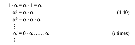
From the definition of above multiplication, we can say that

Hence, we have the following set of elements on which the multiplication operation ‘·’ is defined:

 

 

The element 1 can also be defined as α⁰.

Now we put a condition on the element α so that the set F contains only 2ⁿ elements and is closed under the multiplication ‘·’ defined by Eq. (4.40). We assume p(x) to be a primitive polynomial of degree n over GF(2). Let P(a) = 0. Since p(x) divides x^{2n – 1} + 1, we have 

Substituting x by α in Eq. (4.42), we have 

Since P(α) = 0, we get 

Adding 1 to both sides of Eq. (4.43) and using modulo-2 addition results in 

Therefore, under the condition that P(α) = 0, the set F becomes finite and contains the following elements: 

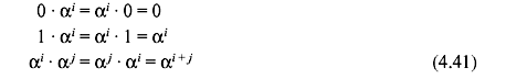
The nonzero elements of F' are closed under the multiplication operation ‘·’ defined by Eq. (4.40). It is shown that the nonzero elements form a commutative group under ‘·’. Again the element 1 is the unit element. Moreover from Eqs. (4.40) and (4.41), it is readily obtained that the multiplication operation is both commutative and associative. For any integer j, where 0 < j < 2ⁿ – 1, α^{2n – j –1} is the multiplicative inverse of α ^j since 

Thus, it follows that 1, α, α²,...,α^{2n – 2} represent 2ⁿ – 1 distinct elements. Hence, the nonzero elements of F' form a group of order 2ⁿ – 1 under the multiplication operation ‘·’ defined by Eq. (4.40).

Now we define an addition operation ‘+’ on F' so that F' forms a commutative group under ‘+’. For 0 < j < 2ⁿ – 1, we divide the polynomial x^j by p(x) and obtain the following:

 

 

where q_j(x) and r_j (x) are the quotient and the remainder, respectively. Remainder r_j(x) is a polynomial of degree (n – 1) or less over GF(2) and has the following form:

 

 

As x and p(x) are relatively prime, x^j is not divisible by p(x). Thus, for any j ≥ 0,

 

 

For 0 ≤ i, j < 2ⁿ – 1, and i ≠ j, it is shown that

 

 

Thus, for j = 0, 1, 2, ..., 2ⁿ – 1, we have 2ⁿ – 1 distinct nonzero polynomials r_j(x) of degree (n – 1) or less. Now replacing x by α in Eq. (4.46), we obtain the following polynomial for α ^j:

Thus, we see that the 2ⁿ – 1 nonzero elements, α⁰, α¹,..., α^{2n – 2} in F', are represented by 2ⁿ – 1 distinct nonzero polynomials of α over GF(2) with degree (n – 1) or less. The zero element 0 in F' can be represented by the zero polynomial. Hence, the 2ⁿ elements in F' are represented by 2ⁿ distinct polynomials of α over GF(2) with degree (n – 1) or less and are regarded as 2ⁿ distinct elements.

Similarly, we can define an addition ‘+’ on F', and it can be shown that the set F' is closed under ‘+’. It can also be verified that F' is a commutative group under ‘+’. Using the polynomial representation for the elements in F', it is readily seen that the multiplication on F' is distributive over the addition on F'. Hence, the set F'= {0, 1, α, α², ..., α^{2n – 2}} is a Galois field of 2ⁿ elements, GF(2ⁿ). Here, it can be observed that the multiplication and addition defined on F' = GF(2ⁿ) imply modulo-2 multiplication and addition. The binary field GF(2) is usually known as the ground field of GF(2ⁿ). The characteristic of GF(2ⁿ) is 4.

Already we have developed two representations for the nonzero elements of GF(2ⁿ)—the power representation and the polynomial representation. Besides, there is another very useful representation for the field elements of GF(2ⁿ). If r₀ + r₁α + r₂α² + r₃α³ + ... + r_{n – 1} α^{n – 1} is a polynomial representation of a field element β, then we can represent β by an ordered sequence of n components, called an n-tuple, as shown:

 

 

where the n components are simply the n coefficients of the polynomial representation of β. There is a one-to-one correspondence between this n-tuple and the polynomial representation of β. The zero element 0 of GF(2ⁿ) is represented by the zero n-tuple (0, 0, 0, ..., 0).

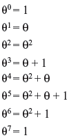
Example 4.6: Construct the Galois field for GF(2³) with n = 3. The primitive polynomial here is P(x) = x³ + x + 1.

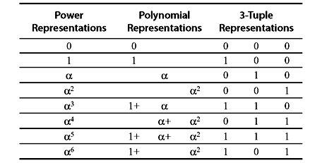
Solution: We set Ρ(α) = 1 + α + α³ = 0. Thus, α³ = 1 + α. Using this we can construct GF(2³). The elements of GF(2³) are shown in Table 4.8. The identity α³ = 1 + α is used repeatedly to form the polynomial representations for the elements of GF(2³). For example,

 

Table 4.8 Three Different Representations for the Elements of GF(2³)

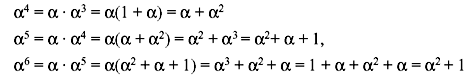
The next power of α is

 

 

Hence, the higher powers of α basically generates one of the existing nonzero elements.

Example 4.7: Find (a) α⁵ + α² + 1 and (b) α⁶ + α³ + α² + α + 1

Solution:

1. From Table 4.8, we can write

    

   α⁵ + α² + 1 = (α² + α + 1) + α² + 1 = α

    

2. Similarly we can write
   

Example 4.8: Find (a) αα⁴, (b) α⁶ α⁴, and (c) α⁶ α⁵ α³

Solution:

1. αα⁴ = α⁵
2. α⁶ α⁴ = α¹⁰ = α⁷α³ = α³
3. α⁶ α⁵ α³ = α¹⁴ = α⁷α⁷ = 1

Example 4.9: Find (a) α⁴/α⁵, (b) 1/α³, (c) α³/α⁴, and (d) α/α⁶

Solution:

1. The inverse of α⁵ is α². Hence, α⁴/α⁵ = α⁴α² = α⁶.
2. Similarly, 1/α³ = α⁴.
3. α³/α⁴ = α³α³ = α⁶.
4. α/α⁶ = αα = α².

4.6  VECTOR SPACES

A vector space V can be defined as a collection of elements, called vectors, together with the operations of vector addition and scalar multiplication which satisfy the following conditions:

1. V is an additive commutative group.
2. For any element a in a field F and any element v in V, a · v in an element in V.
3. For any element v in V and any two elements a and b in a field F, a · (b · v) = (a · b) · v. This is actually the associative law.
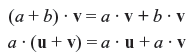
4. For any two elements u and v in V and any elements a and b in a field F,
   
5. If 1 is an unit element of field F, then for any v in V, 1 · v = v.

Now we state some basic properties of vector space as follows:

Property 1: If 0 is the zero element of field F, then for any vector v in V, 0 · v = 0.

Property 2: For any scalar c in F, c · 0 = 0.

Property 3: For any scalar c in F and any vector v in V, (–c) · v = c · (–v) = –(c · v).

In the definition of a vector space, the vectors and scalars can be abstract objects. In fact, the definition does not specify the nature of the vectors or scalars. Here we are most interested in a vector space over GF(2), since it plays a central role in coding theory. We consider an ordered sequence of n components as (v₀,v₁,v₂,...,v_{n – 1}). Here each component v_i is an element from GF(2). Hence, v_i should be either 0 or 1. The sequence shown is generally known as n-tuple over GF(2). The delimiting commas in v can be omitted and we can equally write (v₀v₁v₂ ... v_{n – 1}). Since each v_i can have a choice of two values, 2ⁿ distinct n-tuples can be constructed. Now we denote this set of 2ⁿ distinct n-tuples as V_n. We consider any two vectors from V_n as u = (u₀,u₁,u₂,...,u_{n – 1}) and v = (v₀,v₁,v₂,...,v_{n – 1}). Their sum is given as follows:

where u_i + v_i is carried out in modulo-2 addition and w is also an n-tuple over GF(2). Thus, V_n is closed under the addition operation defined by Eq. (4.50). It can be verified readily that V_n is a commutative group defined by Eq. (4.50). Now we define scalar multiplication of an n-tuple v in V_n by an element a from GF(2) as follows:

where a · v_i is carried out in modulo-2 multiplication. If a = 1, we have

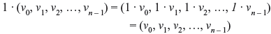
It can also be shown that the vector addition and scalar multiplication defined by Eqs. (4.50) and (4.51), respectively, satisfy the distributive and associative laws. Hence, the set V_n of all n-tuples over GF(2) forms a vector space over GF(2).

Example 4.10: Let n = 4. Construct the vector space V₄ of all 4-tuples over GF(2).

Solution: The vector space V₄ of all 4-tuples over GF(2) consists of 16 vectors, shown as follows:

Now it can be checked that the vector sum of any two vectors from V₄ will result in another element from the same vector space, which only satisfies the closure property of the vector space. Vector space of all n-tuples over any field F can be constructed similarly.

4.6.1  Subspace

It can happen that a subset S of V is also a vector space over F. Such a subset is known as a subspace of V. For any nonempty subspace S of V, the following conditions are satisfied:

1. For any two vectors u and v in S, u + v is also a vector in S.
2. For any element a in F and any vector u in S, a · u is also in S.

4.6.2  Linear Combination

If v₁,v₂,v₃,...,v_m be m vectors in a vector space V over a field, and a₁,a₂,a₃,...,a_m be m scalars from F, then the sum a₁v₁ + a₂v₂ + a₃v₃ + ... + a_mv_m is known as a linear combination of v₁,v₂,v₃,...,v_m. Note  that the set of all linear combinations of v₁,v₂,v₃,...,v_m forms a subspace of V.

A set of vectors v₁,v₂,v₃,...,v_m in a vector space V over a field F is said to be linearly dependent if and only if there exists m scalars a₁, a₂, a₃, ..., a_m from F, not all of them zero, such that

 

 

Alternatively, the set of vectors v₁,v₂,v₃,...,v_m is said to be linearly independent if

 

 

unless a₁ = a₂ = a₃ = ... = a_m = 0.

Example 4.11: For the three sets of vectors determine whether the vectors are linearly dependent or not:

1. u₁ = (4 –9 5), u₂ = (–1 5 13), and u₃ = (–3 –4 –18)
2. v₁ = (14 7 –9), v₂ = (–7 –4 3), and v₃ = (0 2 –6)

Solution:

1. Taking a₁ = 1, a₂ = 1, and a₃ = 1 gives the linear combination
   

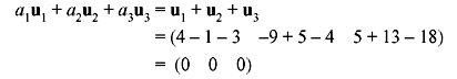
   Hence, the vectors are linearly dependent

2. Taking a₁ = 1, a₂ = 1, and a₃ = 1 gives the linear combination
   

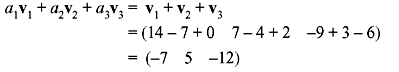
   The resultant vector is nonzero. This does not necessarily mean that the vectors are independent. There can be other scalars that give a zero linear combination. For example, if we take a₁ = 1, a₂ = 2, and a₃ =1/2, then

   

   Thus, the vectors are linearly dependent.

Example 4.12: For the three sets of vectors over GF(2), check whether the vectors are linearly dependent or not:

1. u₁ = (1 0 1 1), u₂ = (0 1 0 0), and u₃ = (1 1 1 1)
2. v₁ = (0 1 1 0), v₂ = (1 0 0 1), and v₃ = (1 0 1 1)

Solution:

1. Taking a₁ = 1, a₂ = 1, and a₃ = 1 gives the linear combination
   

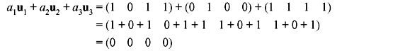
   Hence, the vectors are linearly dependent

2. Taking a₁ = 1, a₂ = 1, and a₃ = 1 gives the linear combination
   

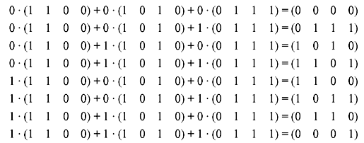
   The resultant vector is nonzero. As shown in the previous example, this does not necessarily mean that the vectors are independent. There can be other scalars that give a zero linear combination. So all of the rest nonzero six linear combinations of these three vectors are checked as follows:

   

Thus, we now find that of all the possible nonzero linear combinations, the resultant vector is nonzero. Hence, the vectors are linearly independent.

4.6.3  Basis (or Base)

In any vector space or subspace, there exists at least one set of linearly independent vectors from which all other vectors can be generated. This set is known as a basis (or base) of the vector space and the vectors of this space are known as basis vectors.

A set of vectors is said to span a vector space V if every vector in V is a linear combination of the vectors in the set. Here, each vector within the vector space can be uniquely expressed as a linear combination of the basis vectors. Hence, the basis vectors are said to span the vector space.

4.6.4  Dimension

The number of vectors within the basis is called the dimension of the vector space. In an n-dimensional vector space, any set of n linearly independent vectors spans the space and is therefore a basis for the space.

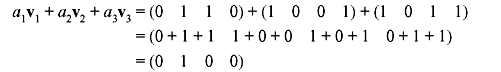
Consider a vector space V_n of all n-tuples over GF(2). The following n n-tuples are formed:

where the n-tuple x_i has only one nonzero component at the ith position. Then every n-tuple (a₀, a₁, a₂, ..., a_{n – 1}) in V_n can be expressed as linear combinations of x₀ x₁, x₂,..., x_{n – 1} as follows:

Hence, x₀, x₁, x₂, ..., x_{n – 1} span the vector space V_n of all n-tuples over GF(2). We also find that x₀, x₁, x₂, ..., x_{n – 1} are linearly independent. Thus, they form a basis for V_n and the dimension of V_n is n. If m < n and v₁, v₂, v₃, ..., v_m are m linearly independent vectors in V_n, then all the linear combinations of v₁, v₂, v₃, ..., v_m of the form

 

 

form an m-dimensional subspace S of V_n. Since each c₁ has two possible values, 0 or 1, there are 2^m possible distinct linear combinations of v₁, v₂, v₃, ..., v_m. Hence, S consists of 2^m vectors and is an m-dimensional subspace of V_n.

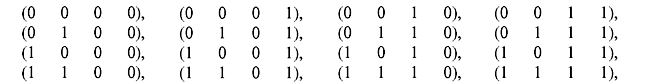
Example 4.13: Determine a basis and the dimension of the subspace in V₄ consisting of the vectors:

Solution: Any two linearly independent nonzero vectors say (1 1 0 0) and (1 0 1 0), can be used as the initial set of vectors. They are linearly independent because if we consider u = a₁(1 1 0 0) + a₂(1 0 1 0) then the only values that give u = 0 are a₁= a₂= 0. Of the remaining five nonzero vectors (0 1 1 0) cannot be appended to the set, since (0 1 1 0) = (1 1 0 0) + (1 0 1 0) and is therefore linearly dependent on the two vectors already in the set.

Any one of the vectors (0 0 0 1), (1 1 0 1), (1 0 1 1) or (0 1 1 1) may be appended to the set. Taking, say, (0 1 1 1) as the third basis vector we find that all the vectors within the subspace can be constructed from a linear combination of the vectors (1 1 0 0), (1 0 1 0), and (0 1 1 1) as follows:

A basis of the subspace is therefore (1 1 0 0), (1 0 1 0), and (0 1 1 1), and the dimension of the subspace is 3, since there are three basis vectors. A point to be noted is that, the basis is not unique. We could have taken (0 0 0 1), (1 1 0 1), and (1 0 1 1) as the third vector to complete the basis.

4.6.5  Orthogonality

Let u = (u₀, u₁, u₂, ..., u_{n – 1})and v = (v₀, v₁, v₂, ..., v_{n – 1}) be two n-tuples in V_n. We define the dot product (or inner product) of u and v as follows:

where u_i · v_i and u_i · v_i + u_{i + 1} · v_{i + 1} are carried out in modulo-2 multiplication and addition. Thus, the inner product u · v is a scalar in GF(2). Two n-tuples u and v are said to be orthogonal to each other, if u · v = 0. Note that orthogonality is a relative property. If u · v = 0, then u and v are orthogonal to each other but not necessarily to other vectors.

It is also possible for a vector in V_n to be orthogonal to itself. For example, let us consider a vector v = (1 1 0 1 1 ) in V₅. The dot product

Hence, (1 1 0 1 1 ) is orthogonal to itself.

Inner product has the following properties:

1. u · v = v · u
2. u · (v + w) = u · v + u · w.
3. (a · u) · v = a (u · v).

4.6.6  Dual Space

Let S be an m-dimensional subspace in V_n and let S_d be the set of vectors in V_n such that, for any u in S and v in S_d, u · v = 0. Thus, the set of vectors in S_d are orthogonal to the vectors in S and is known as the dual space or null space of S. Thus, s · s_d = 0, for all vectors s and s_d belonging to S and S_d, respectively. Conversely S is also the dual space of S_d.

If S is m-dimensional space of the vector space V_n of all n-tuples over GF(2), then the dimension of its dual space S_d is n – m. Alternatively it can be stated that dim(S) + dim(S_d) = n.

Example 4.14: Show that the three-dimensional subspace S of the vector space V₄ consisting of the vectors:

 

 

and the space S_d consisting of

 

 

form dual subspace of V₄. Also determine the dimension of S_d.

 

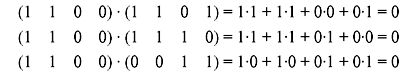
Solution: Taking the dot product of first nonzero vector in S with the nonzero vectors in S_d gives:

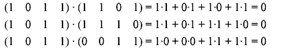
Taking the dot product of second nonzero vector in S with the nonzero vectors in S_d gives:

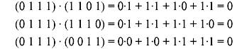
Taking the dot product of third nonzero vector in S with the nonzero vectors in S_d gives:

Thus, we see that all the vectors of S are orthogonal to the vectors in S_d, and therefore S and S_d are dual subspaces of V₄.

In S, the vectors (1 0 1 1) and (0 1 1 1) are linearly independent but the vector (1 1 0 0) = (1 0 1 1) + (0 1 1 1) and hence the dimension of S is 2.

Similarly the vectors (1 1 0 1) and (1 1 1 0) are linearly independent but the vector (0 0 1 1) = (1 1 0 1) + (1 1 1 0) and thus the dimension of the dual space S_d is also 2.

4.7  MATRICES

An m × n matrix over GF(2) (or over any other field) is a rectangular array with m rows and n columns can be written as follows:

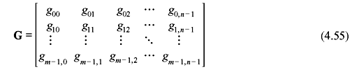
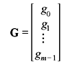
where each entry g_ij with 0 ≤ i < m and 0 ≤ j < n is an element from the binary field GF(2). The first index i indicates the row containing g_ij and the second index j tells the column having g_ij. Often the matrix shown in Eq. (4.55) is written as [g_ij]. We find that each row of G is an n-tuple over GF(2) and each column is a m-tuple over GF(2). The matrix G can be expressed in terms of its m row vectors as follows:

4.7.1  Row Space

If the m (m ≤ n) rows of G are linearly independent, then the 2^m linear combinations of these rows from an m-dimensional subspace of the vector space V_n of all the n-tuples over GF(2). This subspace is called the row space of G.

Example 4.15: Determine the row space of the matrix:

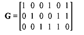
Solution: The row vectors are:

Taking all the 2³ linear combinations of g₁, g₂, and g₃ gives:

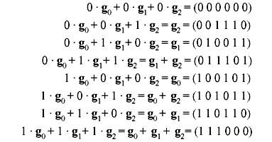
The row space of G therefore contains the vectors:

(0 0 0 0 0 0), (0 0 1 1 1 0), (0 1 0 0 1 1), (0 1 1 1 0 1), (1 0 0 1 0 1), (1 0 1 0 1 1), (1 1 0 1 1 0) and (1 1 1 0 0 0).

We may also express a matrix in terms of column vectors constructed from columns of the matrix, and taking all the linear combinations of the column vectors gives the column space of a matrix. Such a matrix is known as the transpose of G and is usually denoted by G^T. Thus, if G is an m × n matrix over GF(2), then G^T will be an n × m matrix over GF(2). Thus, any matrix G determines two vector spaces–the row vector space and column vector space of G. The dimensions of the column and row vector spaces are known as the column and row rank, respectively. They are the same and referred to as the rank of the matrix.

We can interchange any two rows of G or multiply a row by a nonzero scalar or simply add one row or a multiple of one row to another. These are called elementary row operations. By performing elementary row operations on G, we obtain another matrix G' over GF(2). Both G and G' have the same row space.

Example 4.16: Consider the matrix G in Example 4.15. Adding row 3 to row 1 and then interchanging rows 2 and 3 gives:

Show that the row space generated by G' is the same as that generated by G.

Solution: The row vectors are now (1 0 1 0 1 1), (0 0 1 1 1 0), and (0 1 0 0 1 1). Taking all the eight combinations of these three vectors gives the vectors:

(0 0 0 0 0 0), (0 0 1 1 1 0), (0 1 0 0 1 1), (0 1 1 1 0 1), (1 0 0 1 0 1), (1 0 1 0 1 1), (1 1 0 1 1 0), and (1 1 1 0 0 0).

This is the same set of vectors obtained in Example 4.15 and hence the row spaces generated by G and G' are the same.

Let S be the row space of an m × n matrix G over GF(2) whose m rows g₀, g₁, g₂, ..., g_{m – 1} are linearly independent. Let S_d be the null space of S. In such a case, the dimension of S_d is n – m. Let h₀, h₁, h₂, ..., h_{n – m – 1} be n – m linearly independent vectors in S_d. Obviously these rows span S_d. We can form an (n – m) × n matrix H using h₀, h₁, h₂, ..., h_{n – m – 1} as rows:

The row space of H is S_d. Since each row g_i of G is a vector in S and each row h_j of H is a vector in S_d, the dot product of g_i and h_j must be zero (i.e., g_i · h_j = 0). Since the row space S of G is the null space of the row space S_d of H, we call S the null (or dual) space of H.

Two matrices can be added if they have the same number of rows and the same number of columns. Similarly two matrices can be multiplied if the number of columns in the first matrix is equal to the number of rows in the second matrix. An m × m matrix is called an identity matrix if it has 1’s on the main diagonal and 0’s elsewhere. This matrix is denoted by I_m. A submatrix of a matrix G is a matrix that can be obtained by striking out given rows or columns of G.

4.8  SOLVED PROBLEMS

Problem 4.1: Show that p(x) = x³ + 9x + 6 is irreducible in Q(x). Let θ be a root of p(x). Find the inverse of 1 + θ in Q(θ).

Solution: Irreducibility follows from Eisenstein’s criterion with p = 3. To evaluate 1/(1 + θ), note that we must have 1/(1 + θ) = a + bθ + cθ² for some a, b, c ∊ Q.

Multiplying this out, we find that

 

 

but we also have θ³ = –9θ – 6, so this simplifies to

 

 

Solving for a, b, c gives a = 5/2, b = –1/4, and c = 1/4. Thus,

Problem 4.2: Show that x³ – 2x – 2 is irreducible over Q and let θ be a root. Compute (1 + θ)(1 + θ + θ²) and (1+ θ)/(1 + θ + θ²) in Q(θ).

Solution: This polynomial is irreducible by Eisenstein with p = 2. We perform the multiplication and division just as in the previous problem to get

Problem 4.3 Show that x³ + x + 1 is irreducible over GF(2) and let θ be a root. Compute the powers of θ in GF (2).

Solution: If a cubic polynomial factors, then one of its factors must be linear. Hence, to check that x³ + x + 1 is irreducible over GF(2), it suffices to show that it has no roots in GF(2). Since GF(2) = {0, 1} has only two elements, it is easy to check that this polynomial has no roots. Hence, it is irreducible. For the powers, we have

Problem 4.4: Determine the degree of the extension over Q.

Solution: Since 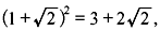we have

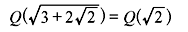
which has degree 2 over Q.

Problem 4.5: Let F ⊂ E be an extension of finite fields. Prove that |E| = |F|^(E/F).

Solution: Let m = (E/F). Choose a basis α₁, ..., α_m in E over F. Every element α ∊ E can be written uniquely as α= b₁α₁ + ... + b_mα_m with b₁, ..., b_m ∊ F. Hence, |E| = |F|^m.

MULTIPLE CHOICE QUESTIONS

1. A (7, 4) linear block code has a rate of
   • 7
   • 4 
   • 1.75
   • 0.571

   Ans. (d)

2. A polynomial is called monic if
   • odd terms are unity 
   • even terms are unity
   • leading coefficient is unity
   • leading coefficient is zero

   Ans. (c)

3. For GF(2³), the elements in the set are
   • {1 2 3 4 5 6 7} 
   • {0 1 2 3 4 5 6}
   • {0 1 2 3 4} 
   • {0 1 2 3 4 5 6 7}

   Ans. (d)

4. What is 5 × 3 – 4 × 2 in Z(6) = {0,1,2,3,4,5}?
   • 1 
   • 2 
   • 3 
   • 4

   Ans. (a)

5. How many solutions are there in Z6 = {0,1,2,3,4,5} of the equation 2x = 0?
   • 2 
   • 1 
   • 3 
   • 4

   Ans. (a)

6. In a go-back-N ARQ, if the window size is 63, what is the range of sequence numbers?
   • 0 to 63 
   • 0 to 64 
   • 1 to 63 
   • 1 to 64

   Ans. (a)

7. ARQ stands for ________.
   • automatic repeat quantization 
   • automatic repeat request
   • automatic retransmission request 
   • acknowledge repeat request

   Ans. (b)

8. In stop-and-wait ARQ, for 10 data packets sent, _______ acknowledgments are needed.
   • exactly 10
   • less than 10
   • more than 10
   • none of the above

   Ans. (a)

9. The stop-and-wait ARQ, the go-back-N ARQ, and the selective-repeat ARQ are for ______ channels.
   • noisy 
   • noiseless 
   • either (a) or (b) 
   • neither (a) nor (b)

   Ans. (a)

10. A = {set of odd integers} and B = {set of even integers}. Find the intersection of A and B.
    • {1,2,3,4,5,7,9} 
    • What the sets have in common
    • { } 
    • {2,4}

    Ans. (c)

11. A burst error means that two or more bits in the data unit have changed
    • double-bit 
    • burst 
    • single-bit
    • none of the above

    Ans. (b)

12. In ______ error correction, the receiver corrects errors without requesting retransmission.
    • backward
    • onward
    • forward 
    • none of the above

    Ans. (c)

13. We can divide coding schemes into two broad categories, ______ and _____ coding.
    • block; linear 
    • linear; nonlinear
    • block; convolution
    • none of the above

    Ans. (c)

14. In modulo-2 arithmetic, ______ give the same results.
    • addition and multiplication
    • addition and division
    • addition and subtraction
    • none of the above

    Ans. (c)

15. In modulo-2 arithmetic, we use the ______ operation for both addition and subtraction.
    • XOR 
    • OR 
    • AND
    • none of the above

    Ans. (a)

16. In modulo-11 arithmetic, we use only the integers in the range _______, inclusive.
    • 1 to 10 
    • 1 to 11 
    • 0 to 10 
    • 0 to 1

    Ans. (c)

17. The ______ of a polynomial is the highest power in the polynomial.
    • range 
    • degree 
    • power 
    • none of these

    Ans. (b)

18. 100110 ⊕ 011011, when ⊕represents modulo-2 addition for binary number, yields
    • 100111 
    • 111101 
    • 000001
    • 011010

    Ans. (b)

Review Questions

1. Compare ARQ and FEC schemes of error control strategies.
2. Calculate the throughput efficiency of the stop-and-wait ARQ system.
3. Draw the block diagram of a typical data transmission system and explain the function of each block.
4. Find the roots of x³ + α⁸x² + α¹²x + α = 0 defined over GF(2⁴).
5. Determine whether the following polynomials over GF(2) are (a) irreducible and (b) primitive:
   
6. Prove that GF(2^m) is a vector space over GF(2).
7. Find all the irreducible polynomials of degree 4 over GF(2).
8. Consider the primitive polynomial p(Z) = Z⁴ + Z + 1 over GF(2). Use this to construct the expansion field GF(16).
9. Given the matrices
   
   

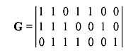
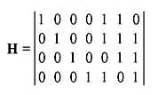
   show that the row space of G is the null space of H, and vice versa.

10. Prove that x⁵ + x³ + 1 is irreducible over GF(2).
11. Let S₁ and S₂ be two subspaces of a vector V. Show that the intersection of S₁ and S₂ is also a subspaces in V.
12. Let V be a vector space over a field F. For any element c in F, prove that c · 0 = 0.
13. Let m be a positive integer. If m is not prime, prove that the set {0, 1, 2, ..., m – 1} is not a field under modulo-m addition and multiplication.
14. Construct the prime field GF(13) with modulo-13 addition and multiplication. Find all the primitive elements and determine the orders of other elements.
15. Construct the vector space V₅ of all 5-tuples over GF(2). Find a three-dimensional subspace and determine its null space.
16. Prove that if β is an element of order n in GF(2^m), all its conjugates have the same order n.