Table of Contents for

Information Theory, Coding and Cryptography

Chapter 3

Source Codes

3.1  INTRODUCTION

In Chapter 2, it has been discussed that both source and channel coding are essential for error-free transmission over a communication channel (Figure 2.1). The task of the source encoder is to transform the source output into a sequence of binary digits (bits) called the information sequence. If the source is a continuous source, it involves analog-to-digital (A/D) conversion. An ideal source encoder should have the following properties:

1. The average bit rate required for representation of the source output should be minimized by reducing the redundancy of the information source.
2. The source output can be reconstructed from the information sequence without any ambiguity.

The channel encoder converts the information sequence into a discrete encoded sequence (also called code word) to combat the noisy environment. A modulator (not shown in the figure) is then used to transform each output symbol of the channel encoder into a suitable waveform for transmission through the noisy channel. At the other end of the channel, a demodulator processes each received waveform and produces an output called the received sequence which can be either discrete or continuous. The channel decoder converts the received sequence into a binary sequence called the estimated sequence. Ideally this should be a replica of information source even in presence of the noise in the channel. The source decoder then transforms the estimated sequence into an estimate of the source output and transfers the estimate to the destination. If the source is continuous, it involves digital-to-analog (D/A) conversion. For a data storage system, a modulator can be considered as a writing unit, a channel as a storage medium and a demodulator as a reading unit. The process of transmission can be compared to recording of data on a storage medium. Efficient representation of symbols leads to compression of data.

In this chapter we will consider various source coding techniques and their possible applications. Source coding is mainly used for compression of data, such as speech, image, video, text, etc.

3.2  CODING PARAMETERS

In Chapter 2, we have seen that the input–output relationship of a channel is specified in terms of either symbols or messages (e.g., the entropy is expressed in terms of bits/message or bits/symbols). In fact, both representations are widely used. In this chapter the following terminology has been used to describe different source coding techniques:

1. Source Alphabet—A discrete information source has a finite set of source symbols as possible outputs. This set of source symbols is called the source alphabet.
2. Symbols or Letters—These are the elements of the source alphabet.
3. Binary Code Word—This is a combination of binary digits (bits) assigned to a symbol.
4. Length of Code Word—The number of bits in the code word is known as the length of code word.

A. Average Code Length   Let us consider a DMS X having finite entropy H(X) and an alphabet {x₁, x₂, ..., x_m} with corresponding probabilities of occurrence P(x_j), where j = 1,2,...,m. If the binary code word assigned to symbol X_j is n_j bits, the average code word length L per source symbol is defined as

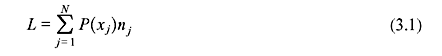
It is the average number of bits per source symbol in the source coding process. L should be minimum for efficient transmission.

B. Code Efficiency   The code efficiency η is given by

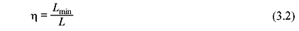
where L_min is the minimum possible value of L. Obviously when η = 1, the code is the most efficient.

C. Code Redundancy   The redundancy γ of a code is defined as

 

3.3  SOURCE CODING THEOREM

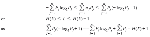
The source coding theorem states that if X be a DMS with entropy H(X), the average code word length L per symbol is bounded as

 

 

L can be made as close to H(X) as desired for a suitably chosen code.

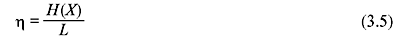
When L_min = H(X),

Example 3.1: A DMS X produces two symbols x₁ and x₂. The corresponding probabilities of occurrence and codes are shown in Table 3.1. Find the code efficiency and code redundancy.

 

Table 3.1 Symbols, Their Probabilities, and Codes

xj	P(xj)	Code
x1	0.8	0
x2	0.2	1

Solution: The average code length per symbol is given by

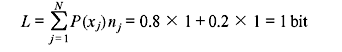
The entropy is

The code efficiency is

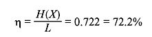
The code redundancy is

 

3.4  CLASSIFICATION OF CODES

A. Fixed-length Codes   If the code word length for a code is fixed, the code is called fixed-length code. A fixed-length code assigns fixed number of bits to the source symbols, irrespective of their statistics of appearance. A typical example of this type of code is the ASCII code for which all source symbols (A to Z, a to z, 0 to 9, punctuation mark, commas etc.) have 7-bit code word.

Let us consider a DMS having source alphabet {x₁, x₂, ..., x_m}. If m is a power of 2, the number of bits required for unique coding is log₂m. When m is not a power of 2, the bits required will be [(log₂m) + 1].

B. Variable-length Codes   For a variable-length code, the code word length is not fixed. We can consider the example of English alphabet consisting of 26 letters (a to z). Some letters such as a, e, etc. appear more frequently in a word or a sentence compared to the letters such as x, q, z, etc. Thus, if we represent the more frequently occurring letters by lesser number of bits and the less frequently occurring letters by larger number of bits, we might require fewer number of bits overall to encode an entire given text than to encode the same with a fixed-length code. When the source symbols are not equiprobable, a variable-length coding technique can be more efficient than a fixed-length coding technique.

C. Distinct Codes   A code is called distinct if each code word is distinguishable from the other. Table 3.2 is an example of distinct code.

 

Table 3.2 Distinct Code

xj	Code Word
x1	00
x2	01
x3	10
x4	11

D. Uniquely Decodable Codes   The coded source symbols are transmitted as a stream of bits. The codes must satisfy some properties so that the receiver can identify the possible symbols from the stream of bits. A distinct code is said to be uniquely decodable if the original source sequence can be reconstructed perfectly from the received encoded binary sequence. We consider four source symbols A, B, C, and D encoded with two different techniques as shown in Table 3.3.

 

Table 3.3 Binary Codes

Symbol	Code 1	Code 2
A	00	0
B	01	1
C	10	00
D	11	01

Code 1 is a fixed-length code, whereas code 2 is a variable-length code. The message ‘A BAD CAB’ can be encoded using the above two codes. In code 1 format, it appears as 00 010011 100001, whereas using code 2 format the sequence will be 0 1001 0001. Code 1 requires 14 bits to encode the message, whereas code 2 requires 9 bits. Although code 2 requires lesser number of bits, yet it does not qualify as a valid code as there is a decoding problem with this code. The sequence 0 1001 0001 can be regrouped in different ways, such as [0] [1][0][0][1] [0][0][01] which stands for ‘A BAAB AAD’ or [0] [1][00][1] [0][0][0][1] which translates to ‘A BCB AAAB’. Since in code 2 format we do not know where the code word of one symbol (letter) ends and where the next one begins it creates an ambiguity; it is not a uniquely decodable code. However, there is no such problem associated with code 1 format since it is a fixed-length code and each group must include 2 bits together. Hence, code 1 format is a uniquely decodable code. In should be noted that a uniquely decodable code can be both fixed-length code and variable-length code.

E. Prefix-free Codes   A code in which no code word forms the prefix of any other code word is called a prefix-free code or prefix code. The coding scheme in Table 3.4 is an example of prefix code.

 

Table 3.4 Prefix Code

Symbol	Code Word
A	0
B	10
C	110
D	1110

We consider a symbol being encoded using code 2 in Table 3.3. If a 0 is received, the receiver cannot decide whether it is the entire code word for alphabet ‘A’ or a partial code word for ‘C’ or ‘D’ that it has received. Hence, no code word should be the prefix of any other code word. This is known as the prefix-free property or prefix condition. The code illustrated in Table 3.4 satisfies this condition.

It is to be mentioned that if no code word forms the prefix of another code word, the code is said to be uniquely decodable. However, the prefix-free condition is not a necessary condition for unique decodability. This is explained in Example 3.2.

F. Instantaneous Codes   A uniquely decodable code is said to be an instantaneous code if the end of any code is recognizable without checking subsequent code symbols. Since the instantaneous codes also have the property that no code word is a prefix of another code word, prefix codes are also called instantaneous codes.

G. Optimal Codes   A code is called an optimal code if it is instantaneous and has minimum average length L for a given source with a particular probability assignment for the source symbols.

H. Entropy Coding   When a variable-length code is designed such that its average code word length approaches the entropy of the DMS, then it is said to be entropy coding. Shannon–Fano coding and Huffman coding (discussed later) are two examples of this type of coding.

Example 3.2: Consider Table 3.5 where a source of size 4 has been encoded in binary codes with 0 and 1. Identify different codes.

 

Table 3.5 Different Binary Codes

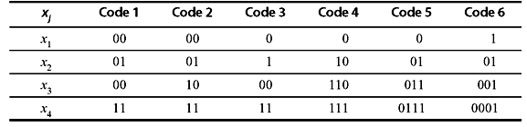
Solution: Code 1 and code 2 are fixed-length codes with length 2.

Codes 3, 4, 5, and 6 are variable-length codes.

All codes except code 1 are distinct codes.

Codes 2, 4, and 6 are prefix (or instantaneous) codes.

Codes 2, 4, and 6 and code 5 are uniquely decodable codes.

(Note that code 5 does not satisfy the prefix-free property, and still it is uniquely decodable since the bit 0 indicates the beginning of each code word.)

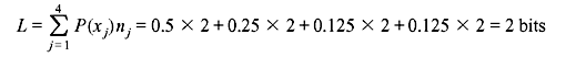
Example 3.3: Consider Table 3.6 illustrating two binary codes having four symbols. Compare their efficiency.

 

Table 3.6 Two Binary Codes

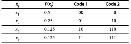
Solution: Code 1 is a fixed-length code having length 2.

In this case, the average code length per symbol is

The entropy is

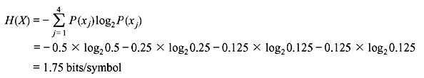
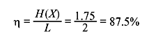
The code efficiency is

Code 2 is a variable-length code.

In this case, the average code length per symbol is

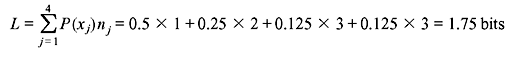
The entropy is

The code efficiency is

Thus, the second coding method is better than the first.

3.5  KRAFT INEQUALITY

Let X be a DMS X having an alphabet {x_j} ( j = 1,2,...,m). If the length of the binary code word corresponding to x_j be n_j, a necessary and sufficient condition for existence of an instantaneous binary code is

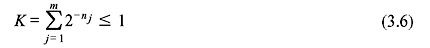
The above expression is known as Kraft inequality. It indicates the existence of an instantaneously decodable code with code word lengths that satisfy the inequality. However, it does not show how to obtain these code words, nor does it tell that any code, for which inequality condition is valid, is automatically uniquely decodable.

Example 3.4: Verify that L ≥ H(X), where L and H(X) are the average code word length per symbol and the source entropy, respectively.

Solution: In Chapter 2, we have shown that (see Problem 2.1)

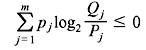
where the equality holds only if Q_j = P_j.

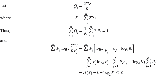
From the Kraft inequality, we get

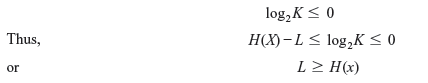
The equality holds if Q_j = P_j and K = 1.

Example 3.5: Consider a DMS with four source symbols encoded with four different binary codes as shown in Table 3.7. Show that

1. all codes except code 2 satisfy the Kraft inequality
2. codes 1 and 4 are uniquely decodable but codes 2 and 3 are not uniquely decodable.

Table 3.7 Different Binary Codes

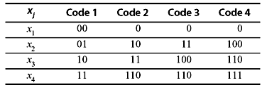
Solution:

1. For code 1: n₁ = n₂ = n₃ = n₄ = 2
   

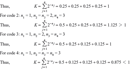
   Hence, all codes except code 2 satisfy Kraft inequality.

2. Codes 1 and 4 are prefix codes; therefore, they are uniquely decodable.

   Code 2 does not satisfy the Kraft inequality. Thus, it is not uniquely decodable.

   Code 3 satisfies the Kraft inequality; yet it is not uniquely decodable. This can be verified considering the following example:

   Let us consider a binary sequence 0110110. Using code 3, this sequence can correspond to x₁x₂x₁x₄ or x₁x₄x₄.

3.6  IMAGE COMPRESSION

Like an electronic communication system, an image compression system contains two distinct functional components: an encoder and a decoder. The encoder performs compression, while the job of the decoder is to execute the complementary operation of decompression. These operations can be implemented by the using a software or a hardware or a combination of both. A codec is a device or a program that performs both coding and decoding operations. In still-image applications, both the encoded input and the decoder output are the functions of two dimensional (2-D) space co-ordinates, whereas video signals are the functions of space co-ordinates as well as time. In general, decoder output may or may not be an exact replica of the encoded input. If it is an exact replica, the compression system is error free, lossless or information preserving, otherwise, the output image is distorted and the compression system is called lossy system.

3.6.1  Image Formats, Containers, and Compression Standards

An image file format is a standard way to organize and store image data. It specifies how the data is arranged and which type of compression technique (if any) is used. An image container is akin to a file format but deals with multiple types of image data. Image compression standards specify the procedures for compressing and decompressing images. Table 3.8 provides a list of the image compression standards, file formats, and containers presently used.

 

Table 3.8 Image Compression Standards, Formats, and Containers

Still image		Video
Binary	Continuous tone	DV (Digital Video)
CCITT Group 3 (Consultative Committee of the International Telephone and Telegraph standard)	JPEG (Joint Photographic Experts Group standard)	H.261
CCITT Group 4	JPEG-LS (Loss less or near loss less JPEG)	H.262
JBIG (or JBIG1) (Joint Bi-level Image Experts Group standard)	JPEG-2000	H.263
JBIG2	BMP (Windows Bitmap)	H.264
TIFF (Tagged Image File Format)	GIF (Graphic Interchange Format)	MPEG-1 (Motion Pictures Expert Group standard)
	PDF (Portable Document Format)	MPEG-2
	PNG (Portable Network Graphics)	MPEG-4
	TIFF	MPEG-4 AVC (MPEG-4 Part 10 Advanced Video Coding)
		AVS (Audio-Video Standard)
		HDV (High-Defi nition Video)
		M-JPEG (Motion JPEG)
		Quick Time
		VC-1 (or WMV9)

3.7  SPEECH AND AUDIO CODING

Digital audio technology forms an essential part of multimedia standards and technology. The technology has developed rapidly over the last two decades. Digital audio finds applications in multiple domains such as CD/DVD storage, digital telephony, satellite broadcasting, consumer electronics, etc.

Based on their applications, audio signals can be broadly classified into three following subcategories:

1. Telephone Speech—This is a low bandwidth application. It covers the frequency range of 300–3400 Hz. Though the intelligibility and naturalness of this type of signal are poor, it is widely used in telephony and some video telephony services.
2. Wideband Speech—It covers a bandwidth of 50–7000 Hz for improved speech quality.
3. Wideband Audio—Wideband audio includes high fidelity audio (speech as well as music) applications. It requires a bandwidth of at least 20 kHz for digital audio storage and broadcast applications.

The conventional digital format for these signals is the Pulse Code Modulation (PCM). Earlier, the compact disc (CD) quality stereo audio was used as a standard for digital audio representation having sampling frequency 44.1 kHz and 16 bits/sample for each of the two stereo channels. Thus, the stereo net bit rate required is 2 × 16 × 44.1 = 1.41 Mbps. However, the CD needs a significant overhead (extra bits) for synchronization and error correction, resulting in a 49-bit representation of each 16-bit audio sample. Hence, the total stereo bit rate requirement is 1.41 × 49/16 = 4.32 Mbps.

Although high bandwidth channels are available, it is necessary to achieve compression for low bit rate applications in cost-effective storage and transmission. In many applications such as mobile radio, channels have limited capacity and efficient bandwidth compression must be employed.

Speech compression is often referred to as speech coding, a method for reducing the amount of information needed to represent a speech signal. Most of the speech-coding schemes are usually based on a lossy algorithm. Lossy algorithms are considered acceptable as far as the loss of quality is undetectable to the human ear. Speech coding or compression is usually implemented by the use of voice coders or vocoders. There are two types of vocoders as follows:

1. Waveform-following Coders—Waveform-following coders exactly reproduce the original speech signal if there is no quantization error.
2. Model-based Coders—Model-based coders cannot reproduce the original speech signal even in absence of quantization error, because they employ a parametric model of speech production which involves encoding and transmitting the parameters, not the signal.

One of the model-based coders is Linear Predictive Coding (LPC) vocoder, which is lossy regardless of the presence of quantization error. All vocoders have the following attributes:

1. Bit Rate—It is used to determine the degree of compression that a vocoder achieves. Uncompressed speech is usually transmitted at a rate of 64 kbps using 8 bits/sample and 8 kHz sampling frequency. Any bit rate below 64 kbps is considered compression. The linear predictive coder transmits the signal at a bit rate of 2.4 kbps.
2. Delay—It is involved with the transmission of an encoded speech signal. Any delay that is greater than 300 ms is considered unacceptable.
3. Complexity—The complexity of algorithm affects both the cost and the power of the vocoder. LPC is very complex as it has high compression rate and involves execution of millions of instructions per second.
4. Quality—Quality is a subjective attribute and it depends on how the speech sounds to a given listener.

Any voice coder, regardless of the algorithm it exploits, will have to make trade-offs between these attributes.

3.8  SHANNON–FANO CODING

Shannon–Fano coding, named after Claude Shannon and Robert Fano, is a source coding technique for constructing a prefix code based on a set of symbols and their probabilities. It is suboptimal as it does not achieve the lowest possible expected code word length like Huffman coding.

Shannon–Fano algorithm produces fairly efficient variable-length encoding. However, it does not always produce optimal prefix codes. Hence, the technique is not widely used. It is used in the IMPLODE compression method, which is a part of the ZIP file format, where a simple algorithm with high performance and the minimum requirements for programming is desired.

The steps or algorithm of Shannon–Fano algorithm for generating source code are presented as follows:

 

Step 1: Arrange the source symbols in order of decreasing probability. The symbols with equal probabilities can be listed in any arbitrary order.

Step 2: Divide the set into two such that the sum of the probabilities in each set is the same or nearly the same.

Step 3: Assign 0 to the upper set and 1 to the lower set.

Step 4: Repeat steps 2 and 3 until each subset contains a single symbol.

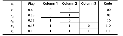
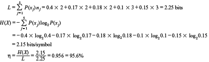
Example 3.6: A DMS X has five symbols x₁, x₂, x₃, x₄, and x₅ with P(x₁) = 0.4, P(x₂) = 0.17, P(x₃) = 0.18, P(x₄) = 0.1, and P(x₅) = 0.15, respectively.

1. Construct a Shannon–Fano code for X.
2. Calculate the efficiency of the code.

Solution:

1. The Shannon–Fano code for X is constructed in Table 3.9.

    

   Table 3.9 Construction of Shannon-Fano Code

   
2. 

3.9  HUFFMAN CODING

Huffman coding produces prefix codes that always achieve the lowest possible average code word length. Thus, it is an optimal code which has the highest efficiency or the lowest redundancy. Hence, it is also known as the minimum redundancy code or optimum code.

Huffman codes are used in CCITT, JBIG2, JPEG, MPEG-1/2/4, H.261, H.262, H.263, H.264, etc.

The procedure of the Huffman encoding is as follows:

 

Step 1: List the source symbols in order of decreasing probability. The symbols with equal probabilities can be arranged in any arbitrary order.

Step 2: Combine the probabilities of the symbols having the smallest probabilities. Now, reorder the resultant probabilities. This process is called reduction 1. The same process is repeated until there are exactly two ordered probabilities remaining. Final step is called the last reduction.

Step 3: Start encoding with the last reduction. Assign 0 as the first digit in the code words for all the source symbols associated with the first probability of the last reduction. Then assign 1 to the second probability.

Step 4: Now go back to the previous reduction step. Assign 0 and 1 to the second digit for the two probabilities that was combined in this reduction step, retaining all assignments made in step 3.

Step 5: Repeat step 4 until the first column is reached.

Example 3.7: Repeat Example 3.6 for the Huffman code and compare their efficiency.

Solution: The Huffman code is constructed in Table 3.10.

 

Table 3.10 Construction of Huffman Code

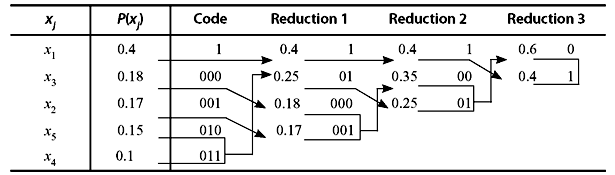
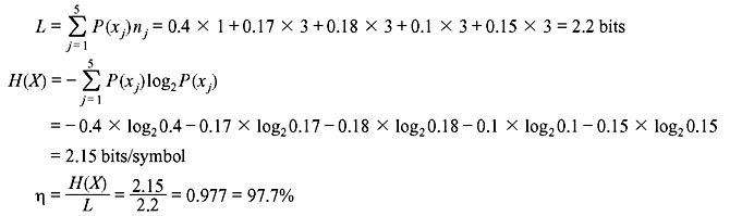
The average code word length for the Huffman code is shorter than that of the Shannon–Fano code. Hence, the efficiency of Huffman code is higher than that of the Shannon–Fano code.

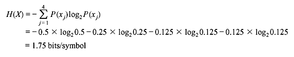
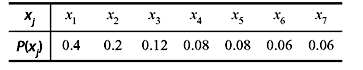
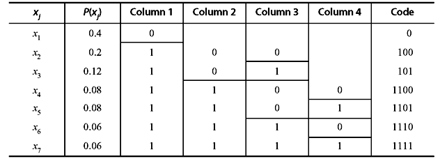
Example 3.8: A DMS X has seven symbols x₁, x₂, x₃, x₄, x₅, x₆, and x₇ with 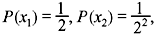respectively.

1. Construct a Huffman code for X.
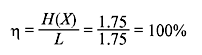
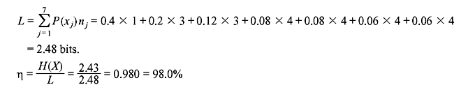
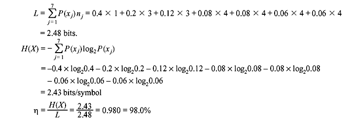
2. Calculate the efficiency of the code.

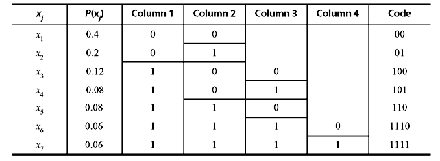
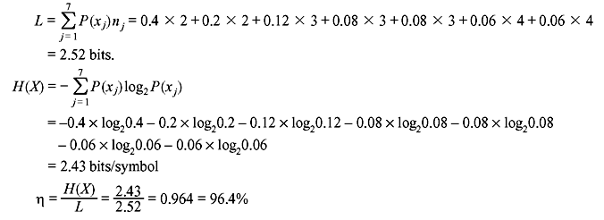
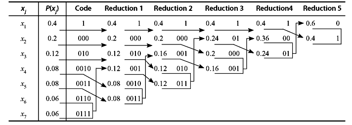
Solution: If we proceed similarly as in the previous example, we can obtain the following Huffman code (see Table 3.11).

 

Table 3.11 Huffman Code for Example 3.8

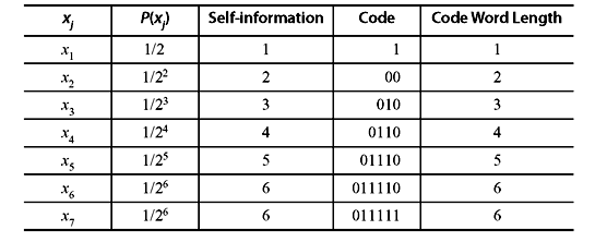
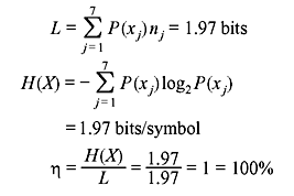
In this case, the efficiency of the code is exactly 100%. It is also interesting to note that the code word length for each symbol is equal to its self-information. Therefore, it can be concluded that to achieve optimality (η = 100%), the self-information of the symbols must be integer, which in turn, requires that the probabilities must negative powers of 2.

3.10  ARITHMETIC CODING

It has been already been shown that the Huffman codes are optimal only when the probabilities of the source symbols are negative powers of two. This condition of probability is not always valid in practical situations. A more efficient way to match the code word lengths to the symbol probabilities is implemented by using arithmetic coding. No one-to-one correspondence between source symbols and code words exists in this coding scheme; instead, an entire sequence of source symbols (message) is assigned a single code word. The arithmetic code word itself defines an interval of real numbers between 0 and 1. If the number of symbols in the message increases, the interval used to represent it becomes narrower. As a result, the number of information units (say, bits) required to represent the interval becomes larger. Each symbol in the message reduces the interval in accordance with its probability of occurrence. The more likely symbols reduce the range by less, and therefore add fewer bits to the message.

Arithmetic coding finds applications in JBIG1, JBIG2, JPEG-2000, H.264, MPEG-4 AVC, etc.

Example 3.9: Let an alphabet consist of only four symbols A, B, C, and D with probabilities of occurrence P(A) = 0.2, P(B) = 0.2, P(C) = 0.4, and P(D) = 0.2, respectively. Find the arithmetic code for the message ABCCD.

Solution: Table 3.12 illustrates the arithmetic coding process.

 

Table 3.12 Construction of Arithmetic Code

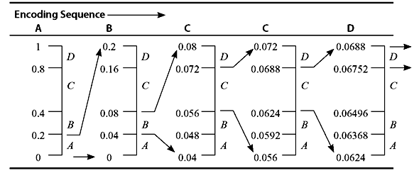
We first divide the interval [0, 1) into four intervals proportional to the probabilities of occurrence of the symbols. The symbol A is thus associated with subinterval [0, 0.2). B, C, and D correspond to [0.2, 0.4), [0.4, 0.8), and [0.8, 1.0), respectively. A is the first symbol of the message being coded, the interval is narrowed to [0, 0.2). Now, this range is expanded to the full height of the figure with its end points labelled as 0 and 0.2 and subdivided in accordance with the original source symbol probabilities. The next symbol B of the message now corresponds to [0.04, 0.08). We repeat the process to find the intervals for the subsequent symbols. The third symbol C further narrows the range to [0.056, 0.072). The fourth symbol C corresponds to [0.06752, 0.0688). The final message symbol D narrows the subinterval to [0.06752, 0.688). Any number within this range (say, 0.0685) can be used to represent the message.

3.11  LEMPEL–ZIV–WELCH CODING

There are many compression algorithms that use a dictionary or code book, known to the coder and the decoder. This dictionary is generated during the coding and decoding processes. Many of these algorithms are based on the work reported by Abraham Lempel and Jacob Ziv, and are known as Lempel–Ziv encoders. In principle, these coders replace repeated occurrences of a string by references to an earlier occurrence. The dictionary is basically the collection of these earlier occurrences. In a written text, groups of letters such as ‘th’, ‘ing’, ‘qu’, etc. appear many times. A dictionary-based coding scheme in this case can be proved effective.

One widely used LZ algorithm is the Lempel–Ziv–Welch (LZW) algorithm reported by Terry A. Welch. It is a lossless or reversible compression. Unlike Huffman coding, LZW coding requires no a priori knowledge of the probability of occurrences of the symbols to be encoded. It is used in variety of mainstream imaging file formats, including GIFF, TIFF and PDF.

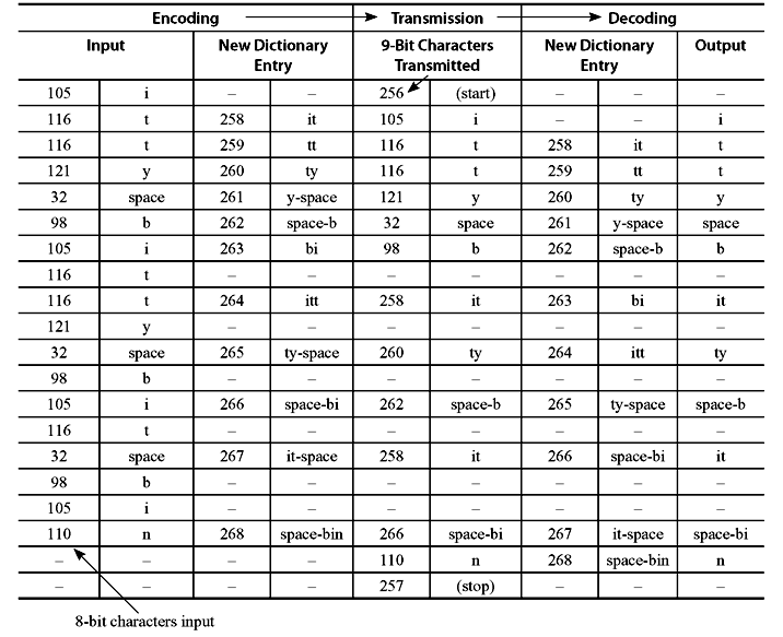
Example 3.10: Encode and decode the following text message using LZW coding:

 

Solution: The initial set of dictionary entries is a 8-bit character code having values 0-255, with ASCII as the first 128 characters, including specifically the following which appear in the string.

 

Table 3.13 LZW Coding Dictionary

Value	Character
32	Space
98	b
105	i
110	n
116	t
121	y

Dictionary entries 256 and 257 are reserved for the ‘clear dictionary’ and ‘end of transmission’ commands, respectively. During encoding and decoding process, new dictionary entries are created using all phrases present in the text that are not yet in the dictionary. Encoding algorithm is as follows.

Accumulate characters of the message until the string does not match any dictionary entry. Then define this string as a new entry, but send the entry corresponding to the string without the last character, which will be used as the first character of the next string to match.

In the given text message, the first character is ‘i’ and the string consisting of just that character is already present in the dictionary. So the next character is added, and the accumulated string becomes ‘it’. This string is not in the dictionary. At this point, ‘i’ is sent and ‘it’ is added to the dictionary, at the next available entry, i.e., 258. The accumulated string is reset to be just the last character, which was not sent, so it is ‘t’. Now, the next character is added; hence, the accumulated string becomes ‘tt’ which is not in the dictionary. The process repeats.

Initially, the additional dictionary entries are all two-character strings. However, the first time one of these two-character strings is repeated, it is sent (using fewer bits than would be required for two characters) and a new three-character dictionary entry is defined. For the given message, it happens with the string ‘itt’. Later, one three-character string gets transmitted, and a four-character dictionary entry is defined.

Decoding algorithm is as follows.

Output the character string whose code is transmitted. For each code transmission, add a new dictionary entry as the previous string plus the first character of the string just received. It is to be noted that the coder and decoder create the dictionary on the fly; the dictionary therefore does not need to be explicitly transmitted, and the coder deals with the text in a single pass.

As seen from Table 3.14, we sent eighteen 8-bit characters (144 bits) in fourteen 9-bit transmissions (126 bits). It is a saving of 12.5% for such a short text message. In practice, larger text files often compress by a factor of 2, and drawings by even more.

 

Table 3.14 Transmission Summary Input

3.12  RUN-LENGTH ENCODING

Run-length encoding (RLE) is used to reduce the size of a repeating string of characters. The repeating string is referred to as a run. It can compress any type of data regardless of its information content. However, content of data affects the compression ratio. Compression ratio, in this case, is not so high. But it is easy to implement and quick to execute. Typically RLE encodes a run of symbols into two bytes, a count and a symbol.

RLE was developed in the 1950s and became, along with its 2-D extensions, the standard compression technique in facsimile (FAX) coding. FAX is a two-colour (black and white) image which is predominantly white. If these images are sampled for conversion into digital data, many horizontal lines are found to be entirely white (long runs of 0’s). Besides, if a given pixel is either black or white, the possibility that the next pixel will match is also very high. The code for a fax machine is actually a combination of a Huffman code and a run-length code. The coding of run-lengths is also used in CCITT, JBIG2, JPEG, M-PEG, MPEG-1/2/4, BMP, etc.

Example 3.11: Consider the following bit stream:

 

Find the run-length code and its compression ratio.

Solution: The stream can be represented as: sixteen 1’s, twenty 0’s and two 1’s, i.e., (16, 1), (20, 0), (2, 1). Since the maximum number of repetitions is 20, which can be represented with 5 bits, we can encode the bit stream as (10000,1), (10100,0), (00010,1).

The compression ratio is 18:38 = 1:2.11.

3.13  MPEG AUDIO AND VIDEO CODING STANDARDS

The Motion Pictures Expert Group (MPEG) of the International Standards Organization (ISO) provides the standards for digital audio coding, as a part of multimedia standards. There are three standards discussed as follows.

A. MPEG-1   In the MPEG-1 standard, out of a total bit rate of 1.5 Mbps for CD quality multimedia storage, 1.2 Mbps is provided to video and 256 kbps is allocated to two-channel audio. It finds applications in web movies, MP3 audio, video CD, etc.

B. MPEG-2   MPEG-2 provides standards for high-quality video (including High-Definition TV) at a rate ranging from 3 to 15 Mbps and above. It also supports new audio features including low bit rate digital audio and multichannel audio. In this case, two to five full bandwidth audio channels are accommodated. The standard also provides a collection of tools known as Advanced Audio Coding (MPEG-2 AAC).

C. MPEG-4   MPEG-4 addresses standardization of audiovisual coding for various applications ranging from mobile access, low-complexity multimedia terminals to high-quality multichannel sound systems with wide range of quality and bit rate, but improved quality mainly at low bit rate. It provides interactivity, universal accessibility, high degree of flexibility, and extensibility. One of its main applications is found in internet audio-video streaming.

3.14  PSYCHOACOUSTIC MODEL OF HUMAN HEARING

The human auditory system (the inner ear) is fairly complicated. Results of numerous psychoacoustic tests reveal that human auditory response system performs short-term critical band analysis and can be modelled as a bank of band pass filters with overlapping frequencies. The power spectrum is not on linear frequency scale and the bandwidths are in the order of 50 to 100 Hz for signals below 500 Hz and up to 5000 Hz at higher frequencies. Such frequency bands of auditory response system are called critical bands. Twenty six critical bands covering frequencies of up to 24 kHz are taken into account.

3.14.1  Masking Phenomenon

It is observed that the ear is less sensitive to low level sound when there is a higher level sound at a nearby frequency. When this occurs, the low level audio signal becomes either less audible or inaudible. This phenomenon is known as masking. The stronger signal that masks the weaker signal is called masker and the weaker one that is masked is known as maskee. It is also found that the masking is the largest in the critical band within which the masker is present and the masking is also slightly effective in the neighbouring bands.

We can define a masking threshold, below which the presence of any audio will be rendered inaudible. It is to be noted that the masking threshold depends upon several factors, such as the sound pressure level (SPL), the frequency of the masker, and the characteristics of the maskee and the masker (e.g., whether the masker or maskee is a tone or noise).

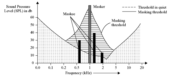
Figure 3.1 Effects of Masking in Presence of a Masker at 1 kHz

In Figure 3.1, the 1-kHz signal acts as a masker. The masking threshold (solid line) falls off sharply as we go away from the masker frequency. The slope of the masking threshold is found to be steeper towards the lower frequencies. Hence, it can be concluded that the lower frequencies are not masked to the extent that the higher frequencies are masked. In the above diagram, the three solid bars represent the maskee frequencies and their respective SPLs are well below the masking threshold. The dotted curve represents quiet threshold in the absence of any masker. The quiet threshold has a lower value in the frequency range from 500 Hz to 5 kHz of the audio spectrum.

The masking characteristics are specified by the following two parameters:

Signal-to-mask ratio (SMR): The SMR at a given frequency is defined as the difference (in dB) between the SPL of the masker and the masking threshold at that frequency.

Mask-to-noise ratio (MNR): The MNR at a given frequency is the difference (in dB) between the masking threshold at that frequency and the noise level. To make the noise inaudible, its level must be below the masking threshold; i.e., the MNR must be positive.

 

Figure 3.2 shows a masking threshold curve. The masking signal appears at a frequency f_m. The SMR, the signal-to-noise ratio (SNR) and the MNR for a particular frequency f corresponding to a noise level have also been shown in the figure. It is evident that

 

 

So far we have considered only one masker. If more than one maskers are present, then each masker has its own masking threshold and a global masking threshold is evaluated that describes just noticeable distortion as a function of frequency.

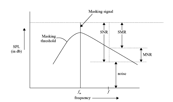
Figure 3.2 Masking Characteristics (SMR and MNR)

3.14.2  Temporal Masking

The masking phenomenon described in the previous subsection is also known as simultaneous masking, where both the masker and the maskee appear simultaneously. Masking can also be observed when two sounds occur within a small interval of time, the stronger signal being masker and the weaker one being maskee. This phenomenon is referred to as temporal masking. Like simultaneous masking, temporal masking plays an important role in human auditory perception. Temporal masking is also possible even when the maskee precedes the masker by a short time interval and is associated with premasking and postmasking, where the former has less than one-tenth duration of that of the latter. The order of postmasking duration is 50–200 ms. Both premasking and postmasking are being used in MPEG audio coding algorithms.

3.14.3  Perceptual Coding in MPEG Audio

An efficient audio source coding algorithm must satisfy the following two conditions:

1. Redundancy removal: It will remove redundant components by exploiting correlations between the adjacent samples.
2. Irrelevance removal: It is perceptually motivated since any sound that our ears cannot hear can be removed.

In irrelevance removal, simultaneous and temporal masking phenomena play major roles in MPEG audio coding. It has already been mentioned that the noise level should be below the masking threshold. Since the quantization noise depends on the number of bits to which the samples are quantized, the bit allocation algorithm must take care of this fact. Figure 3.3 shows the block diagram of a perception-based coder that makes use of the masking phenomenon.

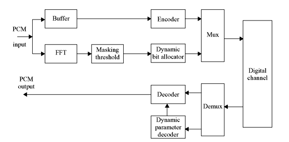
Figure 3.3 Block Diagram of a Perception Based Coder

As seen from the figure, Fast Fourier Transform (FFT) of the incoming PCM audio samples is computed to obtain the complete audio spectrum, from which the tonal components of masking signals can be determined. Using this, a global masking threshold and also the SMR in the entire audio spectrum is evaluated. The dynamic bit allocator uses the SMR information while encoding the bit stream. A coding scheme is called perceptually transparent if the quantization noise is below the global masking threshold. The perceptually transparent encoding process will produce the decoded output indistinguishable from the input.

However, our knowledge in computing the global masking threshold is limited as the perceptual model considers only simple and stationary maskers and sometimes it can fail in practical situations. To solve this problem, sufficient safety margin should be maintained.

3.15  DOLBY

Dolby Digital was first developed in 1992 as a means to allow 35-mm theatrical film prints to store multichannel digital audio directly on the film without sacrificing the standard analog optical soundtrack. It is basically a perceptual audio coding system. Since its introduction the system has been adopted for use with laser disc, DVD-audio, DVD-video, DVD-ROM, Internet audio distribution, ATSC high definition and standard definition digital television, digital cable television and digital satellite broadcast. Dolby Digital is used as an emissions coder that encodes audio for distribution to the consumer. It is not a multigenerational coder which is exploited to encode and decode audio multiple times.

Dolby Digital breaks the entire audio spectrum into narrow bands of frequency using mathematical models derived from the characteristics of the ear and then analyzes each band to determine the audibility of those signals. A greater number of bits represent more audible signals, which, in turn, increases data efficiency. In determining the audibility of signals, the system makes use of masking. As mentioned earlier, a low level audio signal becomes inaudible, if there is a simultaneous occurrence of a stronger audio signal having frequency close to the former. This is known as masking. By taking advantage of this phenomenon, audio signals can be encoded much more efficiently than in other coding systems with comparable audio quality, such as linear PCM. Dolby Digital is an excellent choice for those systems where high audio quality is desired, but bandwidth or storage space is limited. This is especially true for multichannel audio. The compact Dolby Digital bit stream allows full 5.1-channel audio to take less space than a single channel of linear PCM audio.

3.16  LINEAR PREDICTIVE CODING MODEL

Linear predictive coding is a digital method for encoding an analog signal (e.g., speech signal) in which a particular value is predicted by a linear function of the past values of the given signal. The particular source-filter model employed in LPC is known as the linear predictive coding model. It consists of two main components: analysis or encoding and synthesis or decoding. The analysis part involves examining the speech signal and breaking it down into segments or blocks. Each segment is further examined to get the answers to the following key questions:

1. Is the segment voiced or unvoiced? (Voiced sounds are usually vowels and often have high average energy levels. They have very distinct resonant or formant frequencies. Unvoiced sounds are usually consonants and generally have less energy. They have higher frequencies than voiced sounds.)
2. What is the pitch of the segment?
3. What parameters are needed to construct a filter that models the vocal tract for the current segment?

LPC analysis is usually conducted by a sender who is supposed to answer these questions and transmit these answers onto a receiver. The receiver actually performs the task of synthesis. It constructs a filter by using the received answers. When the correct input source is provided, the filter can reproduce the original speech signal.

Essentially, LPC synthesis simulates human speech production. Figure 3.4 illustrates which parts of the receiver correspond to which parts in the human anatomy. In almost all voice coder models, there are two parts: excitation and articulation. Excitation is the type of sound that is transmitted to the filter or vocal tract and articulation is the transformation of the excitation signal into speech.

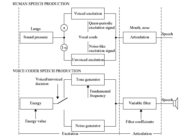
Figure 3.4 Human vs. Voice Coder Speech Production

3.17  SOLVED PROBLEMS

Problem 3.1: Consider a DMS X having a symbol x_j with corresponding probabilities of occurrence P(x_j) = P_j where j = 1,2,...,m. Let n_j be the length of the code word assigned to symbol x_j such that 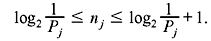Prove that this relationship satisfies the Kraft inequality and find the bound on K in the expression of Kraft inequality.

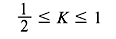
Solution:

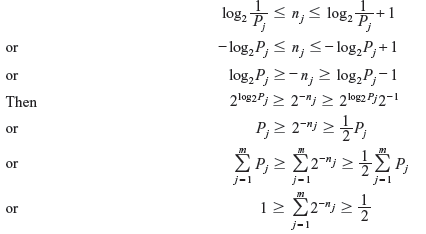
The result indicates that the Kraft inequality is satisfied. The bound on K is

Problem 3.2: Show that a code constructed with code word length satisfying the condition given in Problem 3.1 will satisfy the following relation:

 

 

where H(X) and L are the source entropy and the average code word length, respectively.

Solution: From the previous problem, we have

 

 

Multiplying by P_j and summing over j yields

Problem 3.3: Apply the Shannon–Fano coding procedure for a DMS with the following source symbols and the given probabilities of occurrence. Calculate its efficiency.

 

Table 3.15 Source Symbols and Their Probabilities

Solution:

 

Table 3.16 Construction of Shannon–Fano Code

Another Shannon–Fano code for the same source symbols:

 

Table 3.17 Construction of Another Shannon–Fano Code

The above two procedures reveal that sometimes Shannon–Fano method is ambiguous. The reason behind this ambiguity is the availability of more than one equally valid schemes of partitioning the symbols.

Problem 3.4: Repeat Problem 3.3 for the Huffman code.

Solution:

 

Table 3.18 Construction of Huffman Code

MULTIPLE CHOICE QUESTIONS

1. The coding efficiency is expressed as
   1. 1 + redundancy
   2. 1 – redundancy
   3. 1/redundancy
   4. none of these

   Ans. (b)

2. The code efficiency η is given by
   1. 
   2. 
   3. η = L_min × L
   4. none of these

   Ans. (a)

3. The efficiency of Huffman code is linearly proportional to
   1. average length of code 
   2. average entropy
   3. maximum length of code
   4. none of these

   Ans. (b)

4. In the expression of Kraft inequality, the value of K is given by
   1. 
   2. 
   3. 
   4. 

   Ans. (c)

5. An example of dictionary based coding is
   1. Shannon–Fano coding
   2. Huffman coding
   3. arithmetic coding
   4. LZW coding

   Ans. (d)

6. The run-length code for the bit stream: 11111000011 is
   1. (101,1), (100,0), (010,1)
   2. (101,0), (100,0), (010,1)
   3. (101,1), (100,1), (010,1)
   4. (101,1), (100,0), (010,0)

   Ans. (a)

7. The signal-to-mask ratio (SMR), mask to noise ratio (MNR) and signal to noise ratio (SNR) are related by the formula
   1. SMR (f) = SNR (f) – MNR (f)
   2. SMR (f) = MNR (f) – SNR (f)
   3. SMR (f) = SNR (f) + MNR (f)
   4. none of these

   Ans. (a)

8. Dolby Digital is based on
   1. multigenerational coding
   2. perceptual coding
   3. Shannon–Fano coding
   4. none of these

   Ans. (b)

9. The frequency range of telephone speech is
   1. 4–7 kHz
   2. less than 300 Hz
   3. greater than 20 kHz
   4. 300–3400 Hz

   Ans. (d)

10. LPC is a
    1. waveform-following coder
    2. model-based coder
    3. lossless vocoder
    4. none of these

    Ans. (b)

REVIEW QUESTIONS

1. 1. Define the following terms:
      1. average code length
      2. code efficiency
      3. code redundancy.
   2. State source coding theorem.
2. With suitable example explain the following codes:
   1. fixed-length code
   2. variable-length code
   3. distinct code
   4. uniquely decodable code
   5. prefix-free code
   6. instantaneous code
   7. optimal code.
3. Write short notes on
   1. Shanon–Fano algorithm
   2. Huffman coding
4. 1. Write down the advantages of Huffman coding over Shannon–Fano coding.
   2. A discrete memoryless source has seven symbols with probabilities of occurrences 0.05, 0.15, 0.2, 0.05, 0.15, 0.3 and 0.1. Construct the Huffman code and determine
      1. entropy
      2. average code length
      3. code efficiency.
5. A discrete memoryless source has five symbols with probabilities of occurrences 0.4, 0.19, 0.16, 0.15 and 0.1. Construct both the Shannon–Fano code and Huffman code and compare their code efficiency.
6. With a suitable example explain arithmetic coding. What are the advantages of arithmetic coding scheme over Huffman coding?
7. Encode and decode the following text message using LZW coding:

    

   DAD DADA DAD

    

8. With a suitable example describe run-length encoding.
9. 1. What is masking?
   2. Explain perceptual coding in MPEG audio.
10. Write short notes on
    1. Dolby digital
    2. Linear predictive coding.