Table of Contents for

Information Theory, Coding and Cryptography

Chapter 2

Information Theory

2.1  INTRODUCTION

It is well-known that the performance of any communication system is determined by the available signal power, the presence of undesirable background noise, and limited bandwidth. Naturally, the questions that come to our mind are whether there is any ideal system that can reliably send messages over a communication channel with all its inherent physical limitations and how the message should be represented for reliable transmission over the channel. Recognizing the fact, Claude Shannon developed a completely new theory of communication in 1948 which he called A Mathematical Theory of Communication in which he established the basic theoretical bounds on the performances of communication systems. In his pioneering work, he emphasized that the message should be represented by its information rather than by the signal. His groundbreaking research was soon renamed as Information Theory—a hybrid area of mathematics and engineering. It combines noise protection and efficient use of the channel into a single theory.

Information theory deals with three basic concepts: (a) the measure of source information (the rate at which the source generates the information), (b) the information capacity of a channel (the maximum rate at which reliable transmission of information is possible over a given channel with an arbitrarily small error), and (c) coding (a scheme for efficient utilization of the channel capacity for information transfer). These three concepts are tied together through a series of theorems that form the basis of information theory summarized as follows:

If the rate of information from a message-producing source does not exceed the capacity of the communication channel under consideration, then there exists a coding technique such that the information can be sent over the channel with an arbitrarily small frequency of errors, despite the presence of undesirable noise.

The surprising fact of this statement is that it promises error-free transmission over a noisy communication channel with the aid of coding. Optimum coding matches the source and channel for maximum reliable information transfer, similar to impedance matching for maximum power transfer in electrical circuits. A typical communication system with both source and channel encoding/decoding is shown in Figure 2.1.

The channel encoder/decoder performs the task of error-control coding. An optimum channel coding yields an equivalent noiseless channel with a well-defined capacity of information transmission. The source encoder/decoder is then used to match the source to the equivalent noiseless channel, provided that the source information rate falls within the channel capacity.

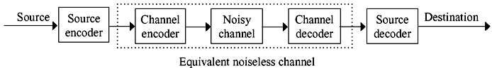
Figure 2.1 A Communication System with Source and Channel Decoding

In this chapter, fundamentals of information theory are discussed in detail. Source coding techniques have been discussed in chapter 3. Various channel coding techniques have been described in chapters 5, 6, 7 and 8.

2.2  MEASURE OF INFORMATION

In a communication system, information is something that is transmitted from the source to the destination, which was previously unavailable to the end user; else nothing would be transferred. Any information source, be it analog or digital, produces message (or event), the outcome of which is selected at random according to a probability distribution. Let us start with the measure of information. Information measures the freedom of choice exercised by the source in selecting a message from many different messages and the user is highly uncertain as to which message will be selected. A message containing knowledge of low probability of occurrence conveys more information than one with a high probability of occurrence. This can be best appreciated with the help of the following example.

One of the basic principles of the media world is: ‘if a dog bites a man, it’s no news, but if a man bites a dog, it’s a news’. The first part, ‘a dog bites a man’, is quite common and seldom constitutes a headline in the newspaper, i.e., it is not a news at all! Technically, the probability of a dog biting a man is rather high; hence, it provides virtually no information. On the contrary, what really catch the reader’s fancy are the last few words, ‘a man bites a dog’. Had a man bitten a dog, it would have occupied the front page of the newspaper. Since the probability of a man biting a dog is almost zero (a rare and unexpected event), a large amount of information is carried by this message. Thus, information is inversely related to the probability of occurrence or directly related to the uncertainty. The less likely the message, the more information it conveys and vice versa.

Let a digital source generate a message m having a probability of occurrence p. The measure of information was quantitatively defined by Shanon as follows:

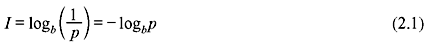
where I is the self-information of the message m, and b is the logarithmic base. Since 0 ≤ p ≤ 1, I ≥ 0, i.e., the information is non-negative. The amount of information in a message depends only on its probability of occurrence rather than its actual content or physical interpretations. Although the probability is a dimensionless quantity, a unit is assigned to I. For the logarithmic base b = 2, the unit of I is bit (binary unit, different from binary digit). When the base is ‘e’, the unit is nat (natural unit), and for b = 10, the unit is decit or Hartley. When no base is mentioned, the unit of the information is taken to as bit, i.e., b = 2. The information given in one unit can be expressed in other unit by the following relationships:

For a discrete memoryless source (DMS), each message emitted is independent of the previous message(s). When such a source sends a number of independent messages m₁, m₂, ..., m_M with their probabilities of occurrence p₁, p₂, ..., p_M, respectively, and the messages are correctly received, the information measure in the composite message is given by

where p₁ + p₂ + ... + p_M = 1.

2.3  ENTROPY

The average information per individual message emitted by a source is known as the entropy of the source. However, the term ‘average information’ is used to indicate ‘statistical average’ and not ‘arithmetic average’. To understand the fact, we consider the following example:

Let us calculate the average mass of M number of students in a class. If the mass of the jth student be m_j (j = 1, 2, ..., M), then the average mass of all students is given by

It can be noted that arithmetic average is applicable for the quantities which are deterministic in nature and hence are to be considered just once. Let us now consider the problem of information associated with every transmitted message (symbol) which is a non-deterministic (probabilistic, statistical) quantity. If there are M messages and the information associated with jth message is I_j , then using the previous definition of arithmetic average the average information per transmitted message is given by

However, the above calculation is wrong as the messages are not transmitted just once; they are transmitted many times and the number of times a message emitted is determined by its probability of occurrence. Hence, the above method is not valid and we adopt the following method to obtain the statistical average.

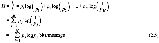
Let us consider M number of different messages m₁, m₂, ..., m_M having their probabilities of occurrences p₁, p₂, ..., p_M, respectively. The source generates a sequence of L-independent messages over a long period of time such that L >> M. The number of messages m₁ within L messages is p₁L and the amount of information in each m₁ is . The total amount of information in all m₁ messages is p₁L . Thus, the total amount of information in all L messages comes out as follows:

and the average information per message or entropy is

If M = 1, i.e., there is only a single possible message and p_j = p = 1, then

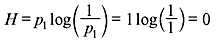
Under such situation, the message carries no information.

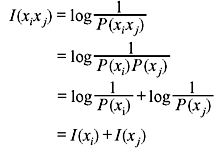
Example 2.1: Verify the equation I(x_ix_j) = I(x_i) + I(x_j), if x_i and x_j are independent.

Solution: As x_i and x_j are independent, P (x_ix_j) = P(x_i)P(x_j)

From Eq. (2.1),

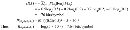
Example 2.2: DMS X produces four symbols x₁, x₂, x₃, and x₄ with probabilities P(x₁) = 0.5, P(x₂) = 0.2, P(x₃) = 0.2, and P(x₄) = 0.1, respectively. Determine H(X). Also obtain the information contained in the message x₄x₃x₁x₁.

Solution:

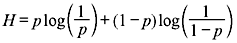
Example 2.3: A binary memoryless system produces two messages with probabilities p and 1 – p. Show that the entropy is maximum when both messages are equiprobable.

Solution:

In order to obtain the maximum source entropy, we differentiate H with respect to p and set it equal to zero.

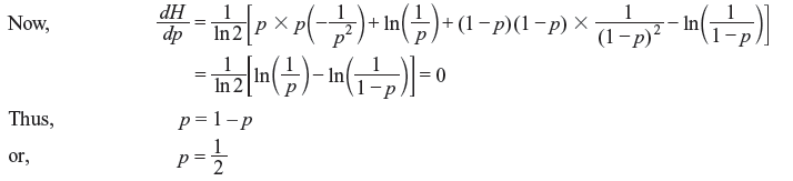
Thus, the entropy is maximum when two messages are equiprobable. It can be shown that the second derivate of H is negative.

The maximum value of the entropy is given by

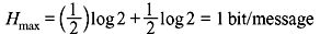
A plot of H as a function of p is shown in Figure 2.2. Note that H is zero for both p = 0 and p = 1.

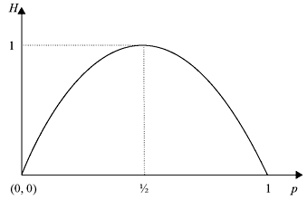
Figure 2.2 Average Information H for Two Messages as a Function of Probability p

Example 2.4: Consider that a digital source sends M independent messages. Show that the source entropy attains a maximum value if all the messages are equally likely.

Solution: Let the respective probabilities of occurrence of the messages be denoted as p₁, p₂, ..., p_M. Then the source entropy

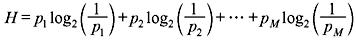
with The partial derivatives ∂H/∂p₁, ∂H/∂p₂, ..., ∂H/∂p_M are equated to zero to get a set of (M – 1) equations. Setting the first partial derivative equal to zero, we obtain

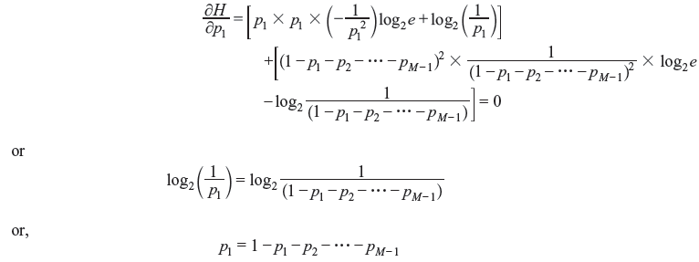
In this way, the (M – 1) equations are obtained as:

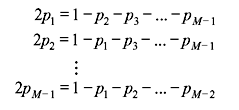
Adding all the above equations,

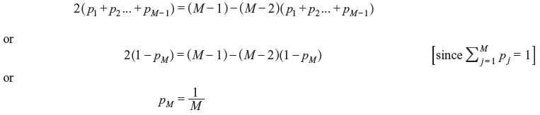
Thus, is the condition that produces 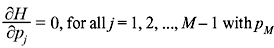being expressed in terms of all other p’s. Similarly, it can be proved that H is maximum when all the messages are equiprobable, i.e., 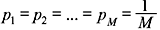and H_max is given by

2.4  INFORMATION RATE

If a source generates r messages/s, the rate of information or the average information per second is defined as follows:

where T is the time required to send a single message

Let there be two sources of equal entropy H, emitting r₁ and r₂ messages/s. The first source emits the information at a rate R₁ = r₁H and the second at a rate R₂ = r₂H. If r₁ > r₂, then R₁ > R₂, i.e., the first source emits more information than the second within a given time period even when the entropy is the same. Therefore, a source should be characterized by its entropy as well as its rate of information.

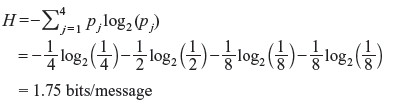
Example 2.5: An event has four possible outcomes with probabilities of occurrence and respectively. Determine the entropy of the system. Also obtain the rate of information if there are 8 outcomes per second.

Solution: The entropy of the system is given by

Thus, the information rate is given by

 

Example 2.6: An analog signal having bandwidth B Hz is sampled at the Nyquist rate and the samples are quantized into four levels Q₁, Q₂, Q₃, and Q₄ with probabilities of occurrence , and respectively. The quantization levels are assumed to be independent. Find the information rate of the source.

Solution: The average information or the entropy is given by

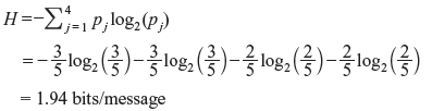
Thus, the information rate is given by

 

2.5  CHANNEL MODEL

A communication channel is the transmission path or medium through which the symbols flow to the receiver. We begin our discussion on channel model with a discrete memoryless channel.

2.5.1  Discrete Memoryless Channel

Figure 2.3 represents a statistical model of a discrete memoryless channel (DMC) with an input X and an output Y. The said channel can accept an input symbol from X, and in response it can deliver an output symbol from Y. Such a channel is ‘discrete’ because the alphabets of X and Y are both finite. Since the present output of the channel solely depends on the current input and not on the inputs at previous stage(s), it is called ‘memoryless’.

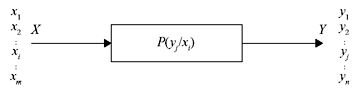
Figure 2.3 Representation of a Discrete Memoryless Channel

The input X of the DMC consists of m input symbols x₁, x₂, ..., x_m and the output Y consists of n output symbols y₁, y₂, ..., y_n. Each possible input-to-output path is related by a conditional probability P(y_j/x_i), where P(y_j/x_i) is the conditional probability of obtaining the output y_j when the input is x_i. P(y_j/x_i) is termed as the channel transition probability.

A channel can be completely specified by a matrix of all such transition probabilities as follows:

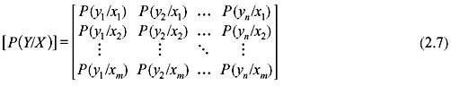
The matrix [P(Y/X)] is called the channel matrix, probability transition matrix or simply transition matrix. As evident from the above matrix, each row contains the conditional probabilities of all possible output symbols for a particular input symbol. As a result, the sum of all elements of each row must be unity, i.e.,

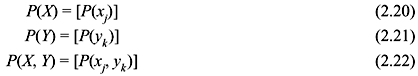
Now, if the input probabilities P(X) are given by the row matrix 

and the output probabilities P(Y) are represented by 

then 

If P(X) is represented as a diagonal matrix

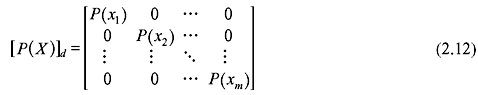
then

where the (i, j) element of [P(X, Y)] is of the form P(x_i, y_j). [P(X, Y)] is known as the joint probability matrix and P(x_i, y_j) is the joint probability of sending x_i and receiving y_j.

2.5.2  Special Channels

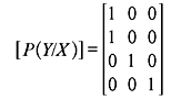
A. Lossless Channel   If the channel matrix of a channel contains only one nonzero element in each column, the channel is defined as a lossless channel. Figure 2.4 shows an example of a lossless channel and the corresponding channel matrix is shown as follows:

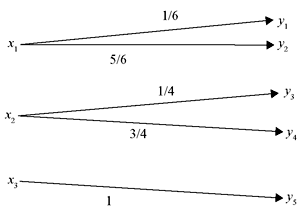
Figure 2.4 A Lossless Channel

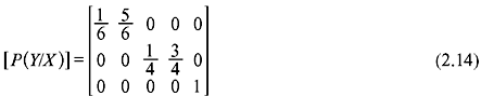
In a lossless channel no source information is lost during transmission.

B. Deterministic Channel   For a deterministic channel, the channel matrix contains only one nonzero element in each row. The following is an example of a channel matrix of a deterministic channel and the corresponding channel representation is shown in Figure 2.5.

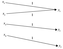
Figure 2.5 A Deterministic Channel

Since each row has only one nonzero element, this element must be unity, i.e., when a particular input symbol is transmitted through this channel, it is known which output symbol will be received.

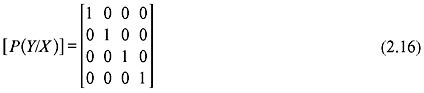
C. Noiseless Channel   A channel is known as noiseless if it is both lossless and deterministic. The corresponding channel matrix has only one element in each row and in each column, and this element must be equal to unity. As the number of input symbols and output symbols is the same (m = n), the channel matrix is a square matrix. Figure 2.6 depicts a typical noiseless channel and corresponding channel matrix is shown in Eq. (2.16).

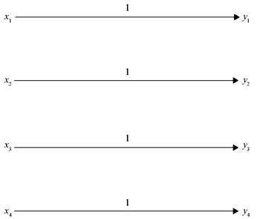
Figure 2.6 A Noiseless Channel

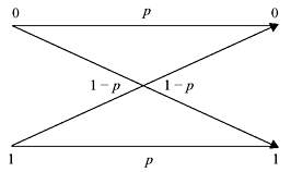
D. Binary Symmetric Channel   A channel described by a channel matrix as shown below is termed a binary symmetric channel (BSC). The corresponding channel diagram is shown in Figure 2.7.

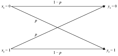
Figure 2.7 A Binary Symmetric Channel

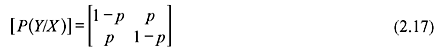
It has two inputs (x₁ = 0, x₂ = 1) and two outputs (y₁ = 0, y₂ = 1). The channel is symmetric as the probability of misinterpreting a transmitted 0 as 1 is the same as that of misinterpreting a transmitted 1 as 0. This common transition probability is denoted by p.

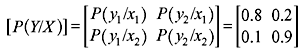
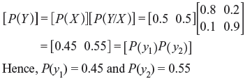
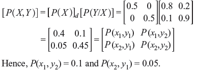
Example 2.7: For the binary channel shown in Figure 2.8, find (a) the channel matrix, (b) P(y₁) and P(y₂) when P(x₁) = P(x₂) = 0.5, and (c) the joint probabilities P(x₁, y₂) and P(x₂, y₁) when P(x₁) = P(x₂) = 0.5.

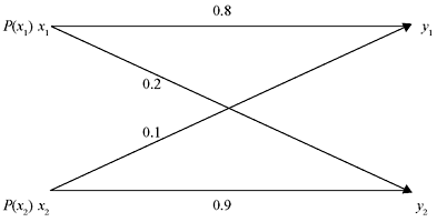
Figure 2.8 A Binary Channel

Solution:

1. The channel matrix is given by
   
2.  
   
3.  
   

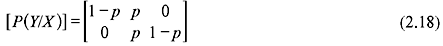
Example 2.8: A channel has been represented by the following channel matrix:

1. Draw the corresponding channel diagram.
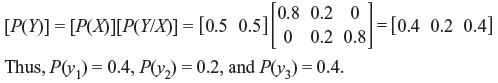
2. If the source produces equally likely outputs, find the probabilities associated with the channel outputs for p = 0.2.

Solution:

1. The channel diagram is shown in Figure 2.9. The channel represented in Eq. (2.18) is known as the binary erasure channel. It has two inputs x₁ = 0 and x₂ = 1 and three outputs y₁ = 0, y₂ = e, and y₃ = 1, where e indicates an erasure; i.e., the output is in doubt and it should be erased.
   

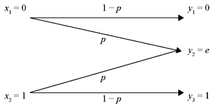
   Figure 2.9 A Binary Erasure Channel

2. 

2.6  JOINT ENTROPY AND CONDITIONAL ENTROPY

We have already discussed the concept of one-dimensional (1-D) probability scheme and its associated entropy. This concept suffices to investigate the behaviour of either the transmitter or the receiver. However, while dealing with the entire communication system we should study the behaviour of both the transmitter and receiver simultaneously. This leads to further extension of the probability theory to two-dimensional (2-D) probability scheme, and, hence, the entropy.

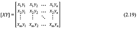
Let the channel input and the channel output form two sets of events [X] = [x₁, x₂, ..., x_m] and [Y] = [y₁, y₂, ..., y_n] with sample spaces S₁ and S₂, respectively, as shown in Figure 2.10. Each event x_j of S₁ produces any event y_k of S₂. Hence, the complete set of events in their product space S (= S₁S₂) is (Figure 2.10) given by

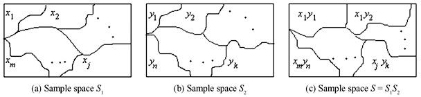
Figure 2.10 Sample Spaces for Channel Input and Output and Respective Their Product Space

Therefore, we have three complete probability schemes and naturally there will be three associated entropies.

(A probability scheme (x_j) is said to be complete if Σ_jΡ(x_j) = 1.) where

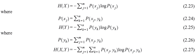
Here, H(X) and H(Y) are marginal entropies of X and Y, respectively, and H(X, Y) is the joint entropy of X and Y. H(X) can be interpreted as the average uncertainty of the channel input and H(Y) the average uncertainty of the channel output. The joint entropy H(X, Y) can be considered as the average uncertainty of the communication channel as a whole.

The conditional probability P(X/Y) is given by

As y_k can occur in conjunction with x₁, x₂, ..., x_m, we have

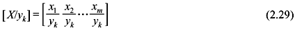
The associated probability scheme can be expressed as follows:

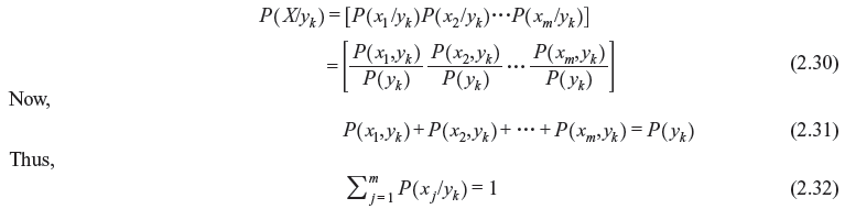
Therefore, the sum of elements of the matrix shown in Eq. (2.30) is unity. Hence, the probability scheme defined by Eq. (2.30) is complete. We can then associate entropy with it.

Thus,

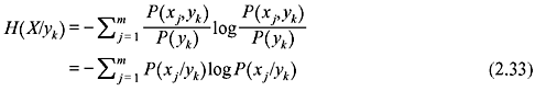
Taking the average of this conditional entropy for all admissible values of y_k we can obtain a measure of an average conditional entropy of the system.

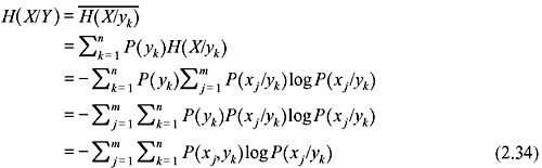
Similarly, it can be shown that

H(X/Y) and H(Y/X) are the average conditional entropies or simply conditional entropies. H(X/Y) is a measure of the average uncertainty remaining about the channel input after the channel output has been observed. It describes how well one can recover the transmitted symbols from the received symbols. H(X/Y) is also called the equivocation of X with respect to Y. H(Y/X) is the average uncertainty of the channel output when X was transmitted and it describes how well we can recover the received symbols from the transmitted symbols; i.e., it provides a measure of error or noise. Finally, we can conclude that there are five entropies associated with a 2-D probability scheme. They are: H(X), H(Y), H(X, Y), H(X/Y) and H(Y/X).

Example 2.9: Show that H(X, Y) = H(X/Y) + H(Y)

Solution:

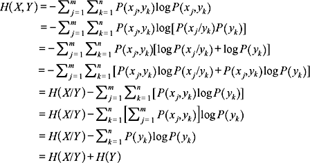
Similarly, it can be proved that H(X, Y) = H(Y/X) + H(X).

Example 2.10: For a lossless channel (Figure 2.4), show that H(X/Y) = 0.

Solution: For a lossless channel when the output y_j is received, it is clear which x_i was transmitted, i.e.,

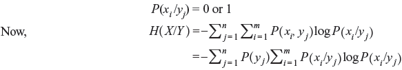
All the terms in the inner summation of the above expression are zero because they are in the form of either 1 × log₂1 or 0 × log₂0. Hence, we can conclude that for a lossless channel

 

 

Example 2.11: For a noiseless channel (Figure 2.6) with m input symbols and m output symbols show that

1. H(X) = H(Y).
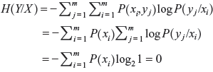
2. H(Y/X) = 0.

Solution:

1. For a noiseless channel the transition probabilities are given by
   
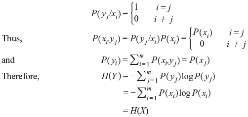
2. We know
   

2.7  MUTUAL INFORMATION

We consider a communication channel with an input X and an output Y. The state of knowledge about a transmitted symbol x_j at the receiver before observing the output is the probability that x_j would be selected for transmission. This is a priori probability P(x_j). Thus, the corresponding uncertainty is –logP(x_j). Once y_k is received at the output, the state of knowledge about x_j is the conditional probability P(x_j /y_k) (also known as a posteriori probability). The corresponding uncertainty becomes –logP(x_j /y_k). Therefore, the information I(x_j; y_k) gathered about x_j after the reception of y_k is the net reduction in the uncertainty, i.e.,

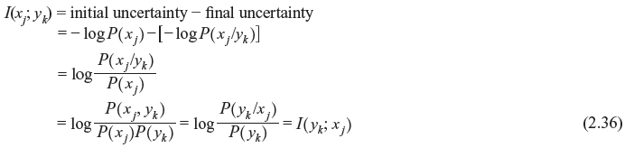
The average of I(x_j; y_k) or the corresponding entropy is given by

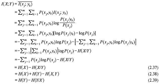
I(X; Y) is known as the mutual information of the channel. It does not depend on the individual symbols x_j or y_k; hence, it is a property of the whole communication channel. The mutual information of a channel can be interpreted as the uncertainty about the channel input that is resolved from the knowledge of the channel output.

The properties of I(X; Y) is summarized as follows:

1. It is non-negative, i.e., I(X; Y) ≥ 0.
2. Mutual information of a channel is symmetric, i.e., I(X; Y) = I(Y; X).
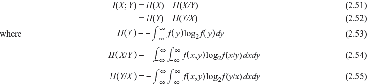
3. It can also be represented as I(X; Y) = H(Y) – H(Y/X).
4. It is related to the joint entropy H(X, Y) by the following formula:

    

   I(X; Y) = H(X) + H(Y) – H(X, Y)

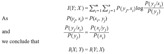
Example 2.12: Verify that I(X; Y) = I(Y; X).

Solution: We can express I(Y; X) as follows:

Example 2.13: Consider a BSC (Figure 2.11) with P(x₁) = α.

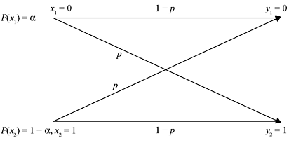
Figure 2.11 A Binary Symmetric Channel with Associated Input Probabilities

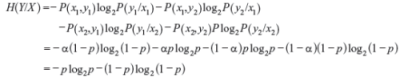
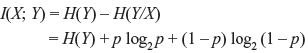
1. Prove that the mutual information I(X; Y) is given by I(X; Y) = H(Y) + p log₂ p + (1 – p) log₂ (1 – p).
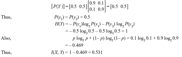
2. Compute I(X; Y) for α = 0.5 and p = 0.1.
3. Repeat (b) for α = 0.5 and p = 0.5 and comment on the result.

Solution:

1. Using Eqs. (2.12), (2.13), and (2.17), we have
   

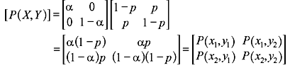
   Then by Eq. (2.35)

   

   Hence,

   
2. When α = 0.5 and p = 0.1, using Eq. (2.11) we have
   
3. When α = 0.5 and p = 0.5, we have
   

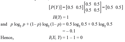
   It is to be noted that when p = 0.5, no information is being transmitted at all. When I(X; Y) = 0, the channel is said to be useless.

2.8  CHANNEL CAPACITY

The channel capacity of a DMC is defined as the maximum of mutual information. Thus, the channel capacity C is given by

where the maximization is obtained with respect to P(x_j).

If r messages are being transmitted per second, the maximum rate of transmission of information per second is rC (bits/s). This is known as the channel capacity per second (sometimes it is denoted as C bits/s).

2.8.1  Special Channels

A. Lossless Channel   For a lossless channel,

Thus,

Therefore, the mutual information is equal to the source entropy and no source information is lost during transmission. As a result, the channel capacity is the lossless channel given by

B. Deterministic Channel   In case of a deterministic channel, H(Y/X) = 0 for all input distributions of P(x_j).

Therefore,

Hence, it can be concluded that the information transfer is equal to the output entropy. The channel capacity is as follows:

where n is total the number of receiver messages.

C. Noiseless Channel   A noise channel is both lossless and deterministic. In this case,

and the channel capacity is given by

D. Binary Symmetric Channel   For a BSC, the mutual information is given by

Since the channel output is binary, H(Y) is maximum when each output has probability of 0.5 and is achieved for equally likely inputs. In this case, H(Y) = 1.

Thus, the channel capacity for such a channel is given by

2.9  SHANNON’S THEOREM

The performance of a communication system for information transmission from a source to the destination depends on a variety of parameters. These include channel bandwidth, signal-to-noise ratio (SNR), probability of bit error, etc. Shannon’s theorem is concerned with the rate of information transfer through a communication channel. According to this theorem, one can transfer information through a communication channel of capacity C (bits/s) with an arbitrarily small probability of error if the source information rate R is less than or equal to C. The statement of the theorem is as follows:

Suppose a source of M equally likely messages (M >> 1) generating information at a rate R. The messages are to be transmitted over a channel with a channel capacity C (bits/s). If R ≤ C, then there exists a coding technique such that the transmitted messages can be received in a receiver with an arbitrarily small probability of error.

Thus, the theorem indicates that even in presence of inevitable noise, error-free transmission is possible if R ≤ C.

2.10  CONTINUOUS CHANNEL

So far we have discussed about the characteristics of discrete channels. However, there are a number of communication systems (amplitude modulation, frequency modulation, etc.) that use continuous sources and continuous channels. In this section, we shall extend the concept of information theory developed for discrete channels to continuous channels. We begin our discussion with the concept of differential entropy.

2.10.1  Differential Entropy

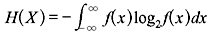
Let an information source produce a continuous signal x(t) to be transmitted through a continuous channel. The set of all possible signals can be considered to be an ensemble of waveforms generated by some ergodic random process. x(t) is also assumed to have finite bandwidth so that it can be completely described by its periodic sample values. At any sampling instant, the collection of possible sample values constitutes a continuous random variable X. If f(x) be the corresponding probability density function (PDF), then the average information per sample value of x(t) is given by

This entropy H(X) is known as the differential entropy of X.

The average mutual information in a continuous channel is given by

2.10.2  Additive White Gaussian Noise Channel

The channels that possess Gaussian noise characteristics are known as Gaussian channels. These channels are often encountered in practice. The results obtained in this case generally provide a lower bound on the performance of a system with non-Gaussian channel. Therefore, if a Gaussian channel with a particular encoder/decoder shows a probability of error p_e, then another encoder/decoder with a non-Gaussian channel can be designed which can yield an error probability less than p_e. Thus, the study of the characteristics of the Gaussian channel is very much essential. The power spectral density of a white noise is constant for all frequencies; i.e, it contains all the frequency components in equal amount. If the probability of occurrence of the white noise level is represented by Gaussian distribution function, it is called white Gaussian noise. For an additive white Gaussian noise (AWGN) channel with input X, the output Y is given by

 

 

where n is an additive band-limited white Gaussian noise with zero mean and variance σ².

2.10.3  Shannon-Hartley Law

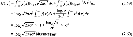
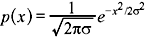
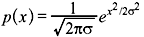
The PDF of Gaussian distribution with zero mean and variance σ² is given by

We know that

Now,

Thus,

Now according to sampling theorem, if a signal is band-limited to B Hz, then it can be completely specified by taking 2B samples per second. Hence, the rate of information transfer is given by

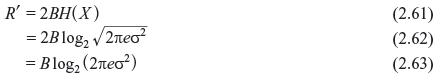
Thus, if f(x) be a band-limited Gaussian noise with an average noise power N (= σ²), then we have

 

 

We now consider the information transfer over a noisy channel emitted by a continuous source. If the channel input and the noise are represented by X and n, respectively, then the joint entropy (in bits/s) of the source and noise is given by

 

 

In practical situation, the transmitted signal and noise are found to be independent to each other. Thus,

 

 

Since, the channel output Y = X + n, we equate

 

 

or

 

 

or

 

 

The rate at which the information is received from a noisy channel is given by

Thus, the channel capacity (in bits/s) is given by

Since R(n) is independent of x(t), maximizing R requires maximizing R(Y).

Let the average power of the transmitted signal be S and that of the white Gaussian noise be N within the bandwidth B of the channel. Then the average power of the received signal will be (S + N). R(Y) is maximum when Y is a Gaussian random process since the noise under consideration is also Gaussian.

Thus,

 

 

Hence, the channel capacity of a band-limited white Gaussian channel is given by

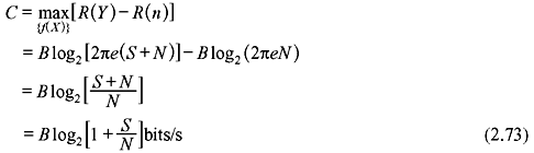
The above expression is known as Shannon–Hartley law. S/N is the SNR at the channel output.

If η/2 be the two-sided power spectral density of the noise in W/Hz, then

Hence,

Example 2.14: Find the capacity of a telephone channel with bandwidth B = 3 kHz and SNR of 40 dB.

Solution:

Example 2.15: Prove that the channel capacity of an ideal AWGN channel with infinite bandwidth is given by

where S and η/2 are the average signal power and the power spectral density of the white Gaussian noise respectively.

Solution: From Eq. (2.75)

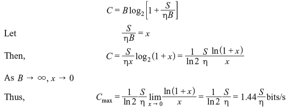
For a fixed signal power and in presence of white Gaussian noise, the channel capacity approaches an upper limit given by expression (2.76) with bandwidth increased to infinity. This is known as Shannon limit.

Example 2.16: Determine the differential entropy H(X) of the uniformly distributed random variable X having PDF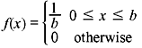

Solution:

2.11  SOLVED PROBLEMS

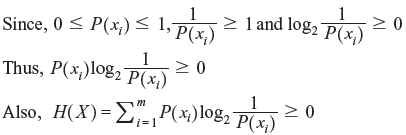
Problem 2.1: Show that 0 ≤ H(X) ≤ log₂m, where m is the size of the alphabet of X.

Solution:

Proof of the lower bound:

It can be noted that , if and only if P(x_i) = 0 or 1.

Since

when, P(x_i) = 1, then P(x_j) = 0 for j ≠ i. Thus, only in this case, H(X) = 0.

Proof of the upper bound:

Let us consider two probability distributions {P(x_i) = P_i} and {Q(x_i) = Q_i} on the alphabet {x_i}, i = 1, 2, ..., m such that

We can write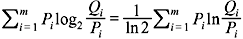

Using the inequality ln α ≤ α – 1, for α ≥ 0 (the equality holds only if α = 1), we get

Thus,

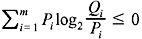(the equality holds only if Q_i= P_i, for all i)

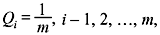Setting we obtain

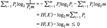
Hence, H(X) ≤ log₂m

The equality holds only if the symbols in X are equiprobable.

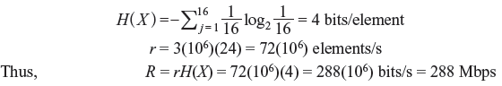
Problem 2.2: A high-resolution B/W TV picture contains 3 × 10⁶ picture elements and 16 different brightness levels. Pictures are repeated at a rate of 24 per second. All levels have equal likelihood of occurrence and all picture elements are assumed to be independent. Find the average rate of information carried by this TV picture source.

Solution:

Problem 2.3: A telegraph source produces two symbols, dash and dot. The dot duration is 0.2 s. The dash duration is 2 times the dot duration. The probability of the dots occurring is twice that of the dash, and the time between symbols is 0.1 s. Determine the information rate of the telegraph source.

Solution:

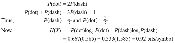
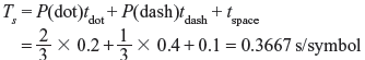
t_dot = 0.2 s, t_dash = 0.4s, and t_space = 0.1 s

Thus, the average time per symbol is given by

and the average symbol rate is

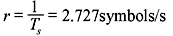
Thus, the average information rate of the telegraph source is given by

 

Problem 2.4: A Gaussian channel has a bandwidth of 1 MHz. Compute the channel capacity if the signal power to noise spectral density ratio (S/η) is 10⁵ Hz. Also calculate the maximum information rate.

Solution:

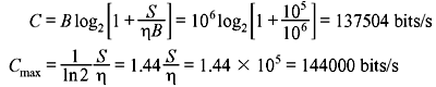
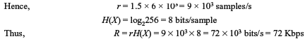
Problem 2.5: An analog signal having 3 kHz bandwidth is sampled at 1.5 times the Nyquist rate. The successive samples are statistically independent. Each sample is quantized into one of 256 equally likely levels.

1. Find the information rate of the source.
2. Is error-free transmission of the output of this source is possible over an AWGN channel with a bandwidth of 10 kHz and SNR of 20 dB.
3. Find the SNR required for error-free transmission for part (b).
4. Determine the bandwidth required for an AWGN channel for error-free transmission of the output of this source when the SNR is 20 dB.

Solution:

1. Nyquist rate = 2 × 3 × 10³ = 6 × 10³ samples/s
   
2. 

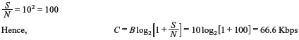
   Since R > C, error-free transmission is not possible.

3. The required SNR can be found by
   

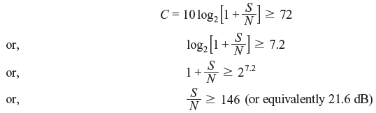
   Hence, the required SNR must be greater than or equal to 21.6 dB for error-free transmission.

4. The required bandwidth can be found as follows:
   

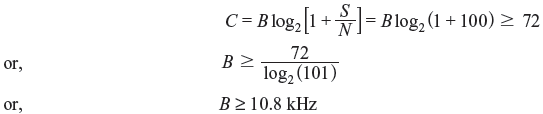
   Hence, the required bandwidth of the channel must be greater than or equal to 10.8 KHz for error-free transmission.

MULTIPLE CHOICE QUESTIONS

1. Entropy represents
   1. amount of information 
   2. rate of information
   3. measure of uncertainty
   4. probability of message

   Ans. (c)

2. 1 nat is equal to
   1. 3.32 bits 
   2. 1.32 bits 
   3. 1.44 bits
   4. 3.44 bits

   Ans. (c)

3. Decit is a unit of
   1. channel capacity 
   2. information
   3. rate of information 
   4. entropy

   Ans. (b)

4. The entropy of information source is maximum when symbol occurrences are
   1. equiprobable 
   2. different probability
   3. both (a) and (b) 
   4. none of these

   Ans. (a)

5. 1 decit equals
   1. 1 bit 
   2. 3.32 bits 
   3. 10 bits 
   4. none of these

   Ans. (b)

6. The ideal communication channel is defined for a system which has
   1. finite C 
   2. BW = 0 
   3. S/N = 0
   4. infinite C.

   Ans. (d)

7. If a telephone channel has a bandwidth of 3000 Hz and the SNR = 20 dB, then the channel capacity is
   1. 3 kbps 
   2. 1.19 kbps 
   3. 2.19 kbps 
   4. 19.97 kbps

   Ans. (d)

8. The channel capacity is a measure of
   1. entropy rate
   2. maximum rate of information a channel can handle
   3. information contents of messages transmitted in a channel
   4. none of these

   Ans. (b)

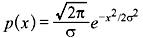
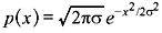
9. Gaussian channel is characterized by a distribution represented by
   1. 
   2. 
   3. 
   4. 

   Ans. (a)

10. The probability of a message is 1/16. The information in bits is
    1. 1 bit
    2. 2 bits
    3. 3 bits 
    4. 4 bits

    Ans. (d)

11. As the bandwidth approaches infinity, the channel capacity becomes
    1. infinite
    2. zero 
    3. 1.44S/η 
    4. none of these

    Ans. (c)

12. Information content in a universally true event is
    1. infinite 
    2. positive constant
    3. negative constant 
    4. zero

    Ans. (d)

13. Following is not a unit of information
    1. Hz 
    2. nat 
    3. decit 
    4. bit

    Ans. (a)

14. The mutual information of a channel with independent input and output is
    1. zero
    2. constant 
    3. variable
    4. infinite

    Ans. (a)

15. The channel capacity of a noise free channel having M symbols is given by
    1. M
    2. log M 
    3. 2^M
    4. none of these

    Ans. (b)

REVIEW QUESTIONS

1. Explain the following terms and their significance:
   • entropy
   • self information
   • mutual information
   • conditional entropy
   • channel capacity
2. 1. Draw the block diagram of a typical message information communication system.
   2. Explain source coding and channel coding.
3. 1. Show that the maximum entropy of a binary system occurs when p = 1/2.
   2. Show that H(X, Y) = H(X/Y) + H(Y).
4. 1. State and prove the Shannon-Hartley law of channel capacity.
   2. A Gaussian channel has a 1 MHz bandwidth. If the signal power-to-noise power spectral density is 10⁵ Hz, calculate the channel capacity and the maximum information transfer rate.
5. 1. Write short note on Shannon’s theorem in communication.
   2. State the channel capacity of a white band-limited Gaussian channel. Derive an expression of noisy channel when bandwidth tends to be very long.
6. 1. What do you mean by entropy of a source?
   2. Consider a source X which produces five symbols with probabilities 1/2, 1/4, 1/8, 1/16 and 1/16. Find the source entropy.
   3. Briefly discuss about the channel capacity of a discrete memoryless channel.

7. For a BSC shown below find the channel capacity for p = 0.9. Derive the formula that you have used.

   
8. A code is composed of dots and dash. Assume that the dash is 3 times as long as the dot and has a one-third the probability of occurrence.
   • Calculate the information in a dot and that in dash.
   •  Calculate the average information in the dot-dash code.
   • Assume that dot lasts for 10 ms and that this same time interval is allowed between symbols. Calculate the average rate of information transmission.
9. For a binary symmetric channel, compute the channel capacity for p = 0.7 and p = 0.4.
10. 1. Verify I(X; Y) ≥ 0.
    2. What do you mean by differential entropy?
    3. Determine the capacity of a telephone channel with bandwidth 3000 Hz and SNR 40 dB.