Table of Contents for

Information Theory, Coding and Cryptography

Chapter 1

Probability, Random Processes, And Noise

1.1  INTRODUCTION

Any signal that can be uniquely described by an explicit mathematical expression, a well-defined rule or a table look-up, is called a deterministic signal. The value of such signals is known or determined precisely at every instant of time. In many practical applications, however, some signals are generated in a random fashion and cannot be explicitly described prior to their occurrence. Such signals are referred to as nondeterministic or random signals. An example of random signal is noise, an ever-present undesirable signal that contaminates the message signal during its passage through a communication link and makes the information erroneous. The composite signal, the desired signal plus interfering noise components at the input of the receiver, is again random in nature. Although there is an uncertainty about the exact nature of the random signals, probabilistic methods can be adopted to present their general behaviour. This chapter aims at presenting a short course on theory of probability, random processes and noise, essential for extracting information-bearing signals from noisy background.

1.2  FUNDAMENTALS OF PROBABILITY

Probability is a measure of certainty. The theory of probability originated from the analysis of certain games of chance, such as roulette and cards. Soon it became a powerful mathematical tool almost in all branches of science and engineering. The following terms are useful in developing the concept of probability:

Experiment—Any process of observation is known as an experiment.

Outcome—It is the result of an experiment.

Random Experiment—An experiment is called a random experiment if its outcome is not unique and therefore cannot be predicted with certainty. Typical examples of a random experiment are tossing a coin, rolling a die or selecting a message from several messages for transmission.

Sample Space, Sample Point and Event—The set S of all possible outcomes of a given random experiment is called the sample space, universal set, or certain event. An element (outcome) in S is known as a sample point or elementary event. An event A is a subset of a sample space (A ⊂ S).

In any random experiment, we are not certain as to whether a particular event will occur or not. As a measure of the probability, we usually assign a number between 0 and 1. If we are sure that the event will occur, the probability of that event is taken as 1 (100%). When the event will never occur, the probability of that event is 0 (0%). If the probability is 9/10, there is a 90% chance that it will occur. In other words, there is a 10% (1/10) probability that the event will not occur.

The probability of an event can be defined by the following two approaches:

1. Mathematical or Classical Probability—If an event can happen in m different ways out of a total number of n possible ways, all of which are equally likely, then the probability of that event is m/n.
2. Statistical or Empirical or Estimated Probability—If an experiment is repeated n times (n being very large) under homogeneous and identical conditions and an event is observed to occur m number of times, then the probability of the event is lim_n→∞ (m/n).

   However, both the approaches have serious drawbacks, as the terms ‘equally likely’ and ‘large number’ are vague. Due to these drawbacks, an axiomatic approach was developed, which is described in Sec. 1.2.2.

1.2.1  Algebra of Probability

We can combine events to form new events using various set operations as follows:

1. The complement of event A(Ā) is the event containing all sample points in S but not in A.
2. The union of events A and B (A ∪ B) is the event containing all sample points in either A or B or both.
3. The intersection of events A and B (A ∩ B) is the event containing all sample points in both A and B.
4. Null or impossible event (Ø) is the event containing no sample point.
5. Two events A and B are called mutually exclusive or disjoint (A ∩ B = Ø) when they contain no common sample point, i.e., A and B cannot occur simultaneously.

Example 1.1: Throw a die and observe the number of dots appearing on the top face. (a) Construct its sample space. (b) If A be the event that an odd number occurs, B that an even number occurs, and C that a prime number occurs, write down their respective subsets. (c) Find the event that an even or a prime number occurs. (d) List the outcomes for the event that an even prime number occurs. (e) Find the event that a prime number does not occur. (f) Find the event that seven dots appear on the top face. (g) Find the event that even and odd numbers occur simultaneously.

Solution:

• Here, the sample space is S = {1,2,3,4,5,6}.

  It has six sample points.

• A = {oddd number} = {1,3,5}

  B = {even number} = {2,4,6}

  C = {prime number} = {2,3,5}.

• B ∪ C = {2,3,4,5,6}.
• B ∩ C = {2}.
• 
• This is a null or impossible event (Ø).
• Since an even and an odd number cannot occur simultaneously, A and B are mutually exclusive (A ∩ B = Ø).

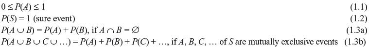
1.2.2  Axioms of Probability

Let P(A) denote the probability of event A of some sample space S. It must satisfy the following axioms:

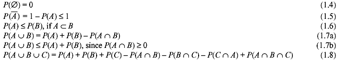
1.2.3  Elementary Theorems on Probability

Some important theorems on probability are as follows:

Example 1.2: Determine the probability for the event that the sum 8 appears in a single throw of a pair of fair dice.

Solution: The sum 8 appears in the following cases:

 

(2,6), (3,5), (4,4), (5,3), (6,2), i.e., 5 cases

Total number of outcomes is 6 × 6 = 36

Thus,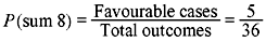     

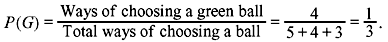
Example 1.3: A ball is drawn at random from a box containing 5 red balls, 4 green balls, and 3 blue balls. Determine the probability that it is (a) green, (b) not green, and (c) red or blue.

Solution:

• Method 1

  Let R, G, and B denote the events of drawing a red ball, green ball, and blue ball, respectively.

  Then        

  Method 2

  The sample space consists of 12 sample points. If we assign equal probabilities 1/12 to each sample point, we again see that P(G) = 4/12 = 1/3, since there are 4 sample points corresponding to green ball.

• 
• Method 1
  

  Method 2

  

  Method 3

  Since events R and G are mutually exclusive, we have

  

Example 1.4: Two cards are drawn at random from a pack of 52 cards. Find the probability that (a) both are hearts and (b) one is heart and one is spade.

Solution: There are ways that 2 cards can be drawn from 52 cards.

• There are ways to draw 2 hearts from 13 hearts.

  Thus, the probability that both cards are hearts =

•  As there are 13 hearts and 13 spades, there are 13 × 13 = 169 ways to draw a heart and a spade.

  Thus, the probability that one is heart and one is spade

Example 1.5: A telegraph source emits two symbols, dash and dot. It was observed that the dash were thrice as likely to occur as dots. Find the probabilities of the dashes and dots occurring.

Solution: We have, P(dash) = 3P(dot).

Now the sum of the probabilities must be 1.

Example 1.6: A digital message is 1000 symbols long. An average of 0.1% symbols received is erroneous. (a) What is the probability of correct reception? (b) How many symbols are correctly received?

Solution:

• The probability of erroneous reception =

  Thus, the probability of correct reception = P(Ā) = 1 − P(A) = 1 − 0.001 = 0.999

• The number of symbols received correctly = 1000 × 0.999 = 999.

1.2.4  Conditional Probability

The conditional probability of an event A given that B has happened (P(A/B)) is defined as follows:

where P(A ∩ B) is the joint probability of A and B.

Similarly,

Using Eqs. (1.9) and (1.10) we can write

or

This is known as Bayes rule.

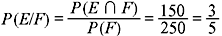
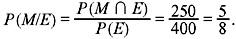
Example 1.7: Consider the following table:

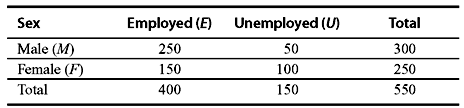
(a) If a person is male, what is the probability that he is unemployed? (b) If a person is female, what is the probability that she is employed? (c) If a person is employed, what is the probability that he is male?

Solution:

• 
• 
• 

1.2.5  Independent Events

Two events A and B are said to be (statistically) independent if

 

 

or

 

 

i.e., the occurrence (or non-occurrence) of event A has no influence on the occurrence (or non-occurrence) of B. Otherwise they are said to be dependent.

Combining Eqs. (1.11) and (1.13), we have

 

 

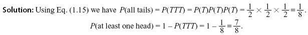
Example 1.8: Determine the probability for the event that at least one head appears in three tosses of a fair coin.

Example 1.9: An experiment consists of observation of five successive pulse positions on a communication link. The pulses can be positive, negative or zero. Also consider that the individual experiments that determine the kind of pulse at each possible position are independent. If the probabilities of occurring a positive pulse and a negative pulse at the ith position (x_i) are p = 0.5 and q = 0.2, respectively, then find (a) the probability that all pulses are negative and (b) the probability that the first two pulses are positive, the next two are zero and the last is negative.

Solution:

• Using Eq. (1.15), the probability that all pulses are negative is given by
  
•  
  

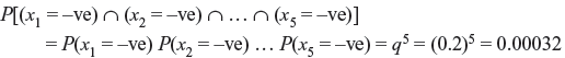
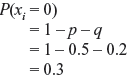
  Hence, the probability that the first two pulses are positive, the next two are zero and the last is negative is given by

  

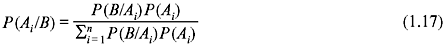
1.2.6  Total Probability

Let A₁, A₂, …, A_n be mutually exclusive (A_i ∩ A_j = Ø, for i ≠ j) and exhaustive 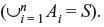Now B is any event in S.

Then

This is known as the total probability of event B.

If A = A_i in Eq. (1.12), then using (1.16) we have the following important theorem (Bayes theorem):

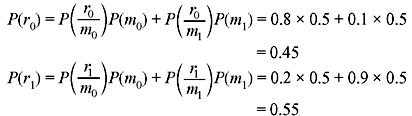
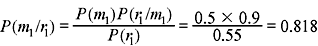
Example 1.10: In a binary communication system (Figure 1.1), either 0 or 1 is transmitted. Due to channel noise, a 1 can be received as 0 and vice versa. Let m₀ and m₁ denote the events of transmitting 0 and 1, respectively. Let r₀ and r₁ denote the events of receiving 0 and 1, respectively. Given P(m₀) = 0.5, P(r₁/m₀) = 0.2 and P(r₀/m₁) = 0.1, (a) find P(r₀) and P(r₁). (b) If a 1 was received, what is the probability that a 1 was sent? (c) If a 0 was received, what is the probability that a 0 was sent? (d) Calculate the probability of error, P_e. (e) Calculate the probability (P_c) that the transmitted signal correctly reaches the receiver.

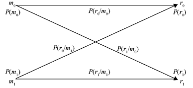
Figure 1.1 A Binary Communication System

Solution:

• We have,
  

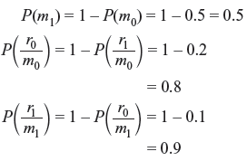
  Using Eq. (1.16), we have

  
• Using Bayes rule (1.12),
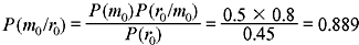
• Proceeding similarly,
• 
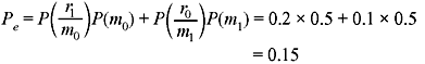
• P_c = 1 − P_e = 1 − 0.15 = 0.85

  This can also be found as follows:

  

1.3  RANDOM VARIABLES AND ITS CHARACTERISTICS

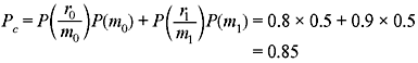
The outcome of an experiment may either be a real number or be a symbol. An example of the former case is the roll of a die and that of the latter is the toss of a coin. However, for meaningful mathematical analysis, it is always convenient to deal with a real number for each possible outcome. Let S [= {s₁, s₂, s₃, …}] be the sample space of some random experiment. A random or stochastic variable X(s_i) (or simply X) is a single-valued real function that assigns a real number to each sample point s_i of S, and the real number is called the value of X(s_i). Schematic diagram representing a random variable (RV) is shown in Figure 1.2.

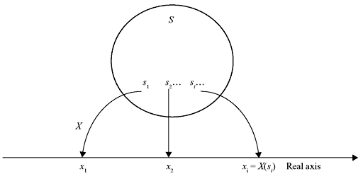
Figure 1.2 The Random Variable X(s)

The sample space S is known as the domain of the RV X, and the collection of all values (numbers) assumed by X is called the range or spectrum of the RV X. RV can be either discrete or continuous.

1. Discrete Random Variable—A random variable is said to be discrete if it takes on a finite or countably infinite number of distinct values. An example of a discrete RV is the number of cars passing through a street in a finite time.
2. Continuous Random Variable—If a random variable assumes any value in some interval or intervals on the real line, then it is called a continuous RV. The spectrum of X in this case is uncountable. An example of this type of variable is the measurement of noise voltage across the terminals of some electronic device.

Example 1.11: Two unbiased coins are tossed. Suppose that RV X represents the number of heads that can come up. Find the values taken by X. Also show schematically the mapping of sample points into real numbers on the real axis.

Solution: The sample space S contains four sample points.

Thus, 

 

 

Table 1.1 illustrates the sample points and the number of heads that can appear (i.e., the values of X). The schematic representation is shown in Figure 1.3.

Figure 1.3 Mapping of Sample Points

 

Table 1.1 Random variable and its values

Outcome	Value of X (Number of Heads)
HH	2
HT	1
TH	1
TT	0

Note that two or more different sample points may assume the same value of X, but two different numbers cannot be assigned to the same sample point.

1.3.1  Discrete Random Variable and Probability Mass Function

Consider a discrete RV X that can assume the values x₁, x₂, x₃, …. Suppose that these values are assumed with probabilities given by

 

 

This function f(x) is called the probability mass function (PMF), discrete probability distribution or probability function of the discrete RV X. f(x) satisfies the following properties:

1. 0 ≤ f(x_i) ≤ 1, i = 1, 2, 3, ….
2. f(x) = 0, if x ≠ x_i (i = 1, 2, 3, …).
3. Σ_i f(x_i) = 1.

Example 1.12: Find the PMF corresponding to the RV X of Example 1.11.

Solution: For the random experiment of tossing two coins, we have

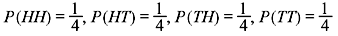
Table 1.2 Tabular Representation of PMF

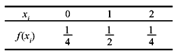
Thus,

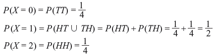
Table 1.2 illustrates the PMF.

1.3.2  Cumulative Distribution Function

The cumulative distribution function (CDF) or briefly the distribution function of a continuous or discrete RV X is given by

The CDF F(x) has the following properties:

1.  0 ≤ F(x) ≤ 1.
2.  F(x) is a monotonic non-decreasing function, i.e., F(x₁) ≤ F(x₂) if x₁ ≤ x₂.
3.  F(−∞) = 0.
4.  F(∞) = 1.
5.  F(x) is continuous from the right, i.e., lim_h→0 + F(x + h) = F(x) for all x.

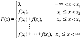
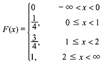
1.3.3  Distribution Function for Discrete Random Variable

The CDF of a discrete RV X is given by

If X assumes only a finite number of values x₁, x₂, x₃, …, then the distribution function can be expressed as follows:

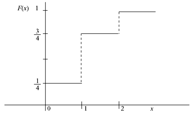
Example 1.13: (a) Find the CDF for the RV X of Example 1.12. (b) Obtain its graph.

Solution:

• The distribution function is
  
•  
  

  Figure 1.4 The CDF

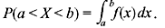
1.3.4  Continuous Random Variable and Probability Density Function

The distribution function of a continuous RV is represented as follows:

where f(x) satisfies the following conditions:

1. f(x) ≥ 0.
2. 
3. 

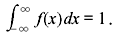
   f(x) is known as the probability density function (PDF) or simply density function.

1.4  STATISTICAL AVERAGES

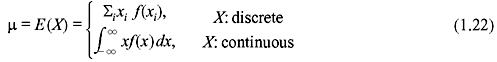
The following terms are important in the analysis of various probability distributions: Expectation—The expectation or mean of an RV X is defined as follows:

Variance and Standard Deviation—The variance of an RV X is expressed as follows:

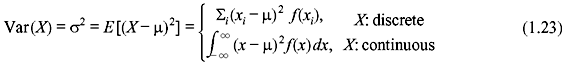
Eq. (1.23) is simplified as follows:

The positive square root of the variance (σ) is called the standard deviation of X.

1.5  FREQUENTLY USED PROBABILITY DISTRIBUTIONS

Several probability distributions are frequently used in communication theory. Among them, binomial distribution, Poisson distribution and Gaussian or normal distribution need special mention.

1.5.1  Binomial Distribution

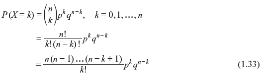
In an experiment of tossing a coin or drawing a card from a pack of 52 cards repeatedly, each toss or selection is called a trial. In some cases, the probability associated with a particular event (such as head on the coin, drawing a heart etc.) is constant in each trial. Such trials are then said to be independent and referred to as Bernoulli trials. Let p be the probability that an event will occur in any single Bernoulli trial (probability of success). Therefore, q = 1 − p is the probability that the event will fail to occur (probability of failure). The probability that the event will occur exactly k times in n trials (i.e. k successes and (n − k) failures) is given by the probability function

where 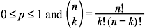is known as the binomial coefficient. The corresponding RV X is called a binomial RV and the CDF of X is

The mean and variance of the binomial RV X are, respectively,

 

 

The binomial distribution finds application in digital transmission, where X stands for the number of errors in a message of n digits.

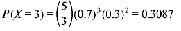
Example 1.14: A binary source generates digits 1 and 0 randomly with probabilities 0.7 and 0.3, respectively. What is the probability that three digits of a five-digit sequence will be 1?

Solution:

1.5.2  Poisson Distribution

Let X be a discrete RV. It is called a Poisson RV if its PMF is expressed as

where α is a positive constant. The above distribution is called the Poisson distribution. The corresponding CDF is given by

The mean and variance in this case are, respectively,

 

 

Poisson distribution finds application in monitoring the number of telephone calls coming at a switching centre during different intervals of time. Binomial distribution fails to solve the problem of the transmission of many data bits, where the error rate is low. In such a situation Poisson distribution proves to be effective.

1.5.3  Gaussian Distribution

The PDF of a Gaussian or normal RV X is given by

where μ and σ are the mean and standard deviation, respectively. The corresponding CDF of X is as follows:

Eq. (1.30) cannot be evaluated analytically and is solved numerically. We define a function Q(z) such that

Thus, Eq. (1.30) is rewritten as follows:

Q(z) is known as the complementary error function. Figure 1.5 illustrates a Gaussian distribution.

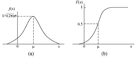
Figure 1.5 Gaussian Distribution

The normal distribution is useful in describing the random phenomena in nature. The sum of a large number of independent random variables, under certain conditions, can also be approximated by a normal distribution (central-limit theorem).

1.6  RANDOM PROCESSES

In the context of communication theory, an RV that is a function of time is called a random process or a stochastic process. Thus, a random process is collection of an infinite number of RVs. Any random signal such as noise is characterized by random process. In order to determine the statistical behaviour of a random process, we might proceed in either of the two ways: We might perform repeated measurement of the same random process or we might take simultaneous measurements of a very large number of identical random processes.

Let us consider a random process such as a noise waveform. To obtain the statistical properties of the noise, we might repeatedly measure the output noise voltage of a single noise source or we might make simultaneous measurements of the output of a very large collection of statistically identical noise sources. The collection of all possible waveforms is known as the ensemble (X(t, s) or simply X(t)), and a waveform in this collection is a sample function or ensemble member or realization of the process.

Stationary Random Process—A random process is called stationary random process if the statistical properties of the process remain unaltered with time.

Strict-Sense Stationary—A random process is said to be strict-sense stationary if its probability density does not change with shift of origin, i.e.,

 

 

Wide-Sense Stationary—A random process is called wide-sense stationary if its mean is a constant and autocorrelation depends only on time difference.

Thus, 

 

 

and

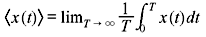
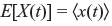
Ergodic Process—A stationary process is known as ergodic process if the ensemble average is equal to the time average. The time-averaged mean of a sample function x(t) of a random process X(t) is given by

Thus, in this case,

The process which is not stationary is termed as non-stationary.

1.7  NOISE

The term noise encompasses all forms of unwanted electrical signal that corrupt the message signal during its transmission or processing in a communication system. Along with other basic factors, it sets limits on the rate of communication. However, it is often possible to suppress or even eliminate the effects of noise by intelligent circuits design. Thus, the study of fundamental sources of noise and their characteristics are very much essential in the context of communication.

1.7.1  Sources of Noise

Noise arises in a variety of ways. Potential sources of random noise can be broadly classified as external noise and internal noise.

1. External Noise—This noise is generated outside the circuit. It can be further classified as
   • Erratic natural disturbances or atmospheric noise or static noise—Natural phenomena that give rise to noise include electric storms, solar flares, lighting discharge during thunderstorm, lightning, intergalactic or other atmospheric disturbances and certain belts of radiation that exist in space. This type of noise occurs irregularly and is unpredictable in nature.

     Noise arising from these sources is difficult to suppress and often the only solution is to reposition the receiving antenna to minimize the received noise, while ensuring that reception of the desired signal is not seriously impaired.

   • Man-made noise—This noise occurs due to the undesired interfering disturbances from electrical appliances, such as motors, switch gears, automobile, fluorescent lighting, leakage from high-voltage transmission line, faulty connection, aircraft ignition, etc. It is difficult to analyze this noise on analytical footing. However, this type of noise is under human control and, in principle, can be eliminated. The frequency range of this noise lies between 1 and 500 MHz.
2. Internal Noise—We are mainly concerned with the noise in the receiver. The noise in the receiving section actually sets lower limit on the size of usefully received signal. Even when ample precautions are taken to eliminate noise caused by external sources, still certain potential sources of noise exist within electronic systems that limit the receiver sensitivity. Use of amplifier to amplify the signal to any desired level may not be of great help because adding amplifiers to receiving system also adds noise and the signal to noise may further be degraded.

   The internal noise is produced by the active and passive electronic components within the communication circuit. It arises due to

   • thermal or Brownian motion of free electrons inside a resistor
   • random emission of electrons from cathode in a vacuum tube, and
   • random diffusion of charge carriers (electrons and holes) in a semiconductor.

     Some of the main constituents of internal noise are thermal noise, shot noise, partition noise and flicker noise.

1.7.2  Thermal Noise

In a conductor, the free electrons are thermally agitated because heat exchange takes place between the conductor and its surroundings. These free electrons exhibit random motion as a result of their collisions with lattice structure. Consequently, there exists a random variation in the electron density throughout the conductor, resulting in a randomly fluctuating voltage across the ends of the conductor. This is the most important class of noise in electronic circuits and known as thermal noise or Johnson noise or resistor noise.

Thermal noise can be best be described by a zero mean Gaussian process and has a flat type of power spectral density over a wide range of frequencies.

1.7.3  Shot Noise

Shot noise appears in all amplifying and active devices as a random fluctuation superimposed on the steady current crossing a potential barrier. The effect occurs because electrical current is not a continuous but discrete flow of charge carriers. In vacuum tubes, shot noise is caused by random emission of electrons from cathode. In semiconductor devices, it is generated due to the random variation in the diffusion of minority carriers (holes and electrons) and random generation and recombination of electron–hole pairs. As lead shots from a gun strike a target, in a similar way, electrons from the cathode strike the anode plate in a vacuum tube; hence, the name shot noise. Although shot noise is always present, its effect is significant in the amplifying devices.

The fluctuating component of current (i_n(t)) which wiggles around the mean value I_dc is the shot noise. Thus, the total current i(t) is expressed as follows:

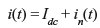
Like thermal noise, shot noise also has flat type of power spectrum (power spectral density) except in the high microwave frequency range. For diodes, the rms shot noise current is given by

where I_dc is the direct diode current, q is the electronic charge (= 1.6 × 10¹⁹ C) and B is the bandwidth of the system.

1.7.4  Partition Noise

Partition noise is generated in multi-grid tubes (tetrode, pentode, etc.) where current divides between two or more electrodes due to random fluctuations of electrons emitted from cathode among various electrodes. In this respect, a diode would be less noisy than a transistor. Hence, the input stage of microwave receivers is often a diode circuit. Very recently, GaAs field effect transistors have been developed for low-noise microwave amplification. The spectrum for partition noise is also flat.

1.7.5  Flicker Noise or 1/f Noise

At low audio frequencies (less than few kilohertz), another type of noise arises in vacuum tubes and semiconductor devices, the power spectral density of which is inversely proportional to frequency. This noise is known as flicker noise or 1/f noise. In vacuum tubes, it stems due to gradual changes in the oxide structure of oxide-coated cathodes and due to the migration of impurity ions through the oxide. In case of semiconductor devices, it is produced due to contaminants and defects in the crystal structure.

1.8  SOLVED PROBLEMS

Problem 1.1: What is the probability that either a 1 or 6 will appear in the experiment involving the rolling of a die?

Solution: Since each of the six outcomes is equally likely in a large number of trials, each outcome has a probability of 1/6.

Thus, the probability of occurrence of either 1 or 6 is given by

Problem 1.2: Consider an experiment of drawing two cards from a deck of cards without replacing the first card drawn. Determine the probability of obtaining two red aces in two draws.

Solution: Let A and B be two events ‘red ace in the first draw’ and ‘red ace in the second draw’, respectively.

We know that P(A ∩ B) = P(A)P(B/A)

The relative frequency of

P(B/A) is the probability of drawing a red ace in the second draw provided that the outcome of the first draw was a red ace.

Problem 1.3: The random variable X assumes the values 0 and 1 with probabilities p and q = 1 − p, respectively. Find the mean and the variance of X.

Solution:

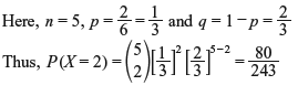
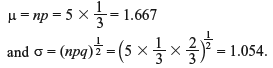
Problem 1.4: A fair die is rolled 5 times. If 1 or 6 appears, it is called success. Determine (a) the probability of two successes and (b) the mean and standard deviation for the number of successes.

Solution: We apply binomial distribution.

• 
• 

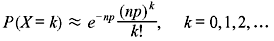
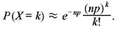
Problem 1.5: When n is very large (n >> k) and p very small (p << 1), prove that the binomial distribution can be approximated by the following Poisson distribution:

Solution: From binomial distribution, we write

Since n >> k and p << 1, then

 

 

and

 

 

Thus, 

 

 

Substituting these values into Eq. (1.33) we get

MULTIPLE CHOICE QUESTIONS

1. Two cards are drawn at random from a pack of 52 cards. The probability that both are spades is
   • 1/15 
   • 2/17 
   • 1/17 
   • 2/15

   Ans. (c)

2. A ball is drawn at random from a box containing 6 red balls, 4 white balls, and 5 blue balls. The probability that it is red is
   • 2/5 
   • 4/15 
   • 1/3 
   • 2/3

   Ans. (a)

3. In the above problem, the probability that the ball is red or white is
   
   • 2/5 
   • 2/3 
   • 7/15 
   • 1/5

   Ans. (b)

4. Three light bulbs are chosen at random from 15 bulbs out of which 5 are defective. The probability that exactly one is defective is
   • 24/91
   • 45/91 
   • 67/91 
   • none of these

   Ans. (b)

5. In the above problem, the probability that none of the three bulbs is defective is
   • 13/91 
   • 67/91 
   • 55/97 
   • 24/91

   Ans. (d)

6. Let A and B be two events with 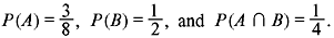The value of P(A ∪ B) is
   • 5/8
   • 1/3 
   • 1/2
   • 3/8

   Ans. (a)

7. The probability of a 4 turning up at least once in two tosses of a fair die is
   • 11/36 
   • 17/36 
   • 13/36 
   • 19/36

   Ans. (a)

8. A class has 12 boys and 4 girls. If three students are selected at random from the class, the probability that they are all boys is
   • 19/28 
   • 3/28 
   • 17/28 
   • 11/28

   Ans. (d)

9. A box contains 7 red marbles and 3 white marbles. Three marbles are drawn from the box one after the other. The probability that the first two are red and the third is white is
   • 1/12
   • 2/9 
   • 7/40 
   • 13/40

   Ans. (c)

10. The expectation of the sum of points in tossing a pair of fair dice is
    • 9
    • 5 
    • 6 
    • 7

    Ans. (d)

11. In the above problem, the variance is
    • 37/6 
    • 35/12 
    • 35/6 
    • none of these

    Ans. (c)

12.  A random variable X has the following density function:
       

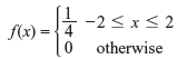
    Var (X) is

    • 1 
    • 2 
    • 3 
    • 4

    Ans. (a)

13. A random variable X has E(X) = 2, E(X²) = 8. The standard deviation is
    • 1 
    • 2 
    • 4 
    • 10

    Ans. (b)

14. A random variable X is such that E[(X − 1)²] = 10, E[(X − 2)²] = 6. E(X) is
    • 7/2 
    • 5/2 
    • 3/2 
    • 8/3

    Ans. (a)

15. In the above problem, Var (X) is
    • 17/4 
    • 15/4 
    • 13/4 
    • none of these

    Ans. (b)

REVIEW QUESTIONS

1. • Define following terms:
     • conditional probability
     •  independent events
     • probability mass function
     • cumulative distribution function
     • probability density function
     • expectation.
   • State Bayes theorem.
2. What is the chance that a leap year selected at random will contain 53 Wednesdays?
3. If A and B are mutually independent events, then show that the following pairs are independent:
   • 
   • 
   • 
4. If A, B and C be mutually independent events, then prove that
   • A and B + C are independent
   • are mutually independent.
5. In a bolt factory, machines A, B, and C manufacture 25%, 35%, and 40% of the total of their output, respectively. Out of them, 5%, 4%, and 2% are defective bolts. A bolt is drawn at random from the product and is found to be defective. What are the probabilities that it was manufactured by machines A, B, and C?
6. A box contains 5 defective and 10 non-defective lamps. Eight lamps are drawn at random in succession without replacement. What is the probability that the eighth lamp is the fifth defective?
7. Three groups of children contain three girls and one boy, two girls and two boys, and one girl and three boys. One child is selected at random from each group. Show that the chance that the three selected children consisting of one girl and two boys is 13/32.
8. Two persons A and B throw alternatively with a pair of dice. A wins if he throws 6 before B throws 7 and B wins if he throws 7 before A throws 6. If A begins, find his probability of winning.
9. A variable X has the density function
   

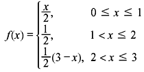
   Find the mean and variance of X.

10. For a random variable X, Var (X) = 1, find Var (2X + 3).
11. If X has binomial distribution with parameter n and p, then show that
    • its mean is np
    • its variance is npq, where q = 1 − p.
12. A car-hire firm has two cars, which it hires out day by day. The number of demands for a car on each day is distributed as a Poisson distribution with average number of demand per day being 1.5. Calculate the proportion of days on which neither car is used and the proportion of days on which some demand is refused (e^−1.5 = 0.2231).
13. If X is normally distributed with zero mean and unit variance, find the expectation of X².
14. If X is a Poisson variate such that P(X = 1) = 0.2 and P(X = 2) = 0.2, find P(X = 0).
15. Show that for a Poisson variate standard deviation =