Intermediate C Programming

332 Intermediate C Programming

{

int val = array[index];39

printf("delete%d\n", val);40

root = Tree_delete(root, val);41

Tree_print(root);42

}43

}44

Tree_destroy(root);45

free (array);46

return EXIT_SUCCESS;47

}48

20.8 Makefile

The following listing is an example Makefile for compiling and running the code under

valgrind.

CFLAGS = -g -Wall -Wshadow

GCC = gcc $(CFLAGS)2

SRCS = treemain.c treesearch.c treedestroy.c treeinsert.c3

SRCS += treeprint.c treedelete.c4

OBJS = $(SRCS:%.c=%.o)5

tree: $(OBJS)7

$(GCC) $(OBJS) -o tree8

memory: tree10

valgrind --leak-check=yes --verbose ./tree 1011

.c.o:13

$(GCC) $(CFLAGS) -c $*.c14

clean:16

rm -f *.o a.out tree17

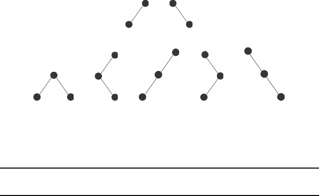
20.9 Counting the Diﬀerent Shapes of a Binary Tree

How many unique shapes can a binary tree with n nodes possibly have? This is the

deﬁnition of shapes. Two binary trees have the same shape if each node has the same

number of left oﬀsprings and the same number of right oﬀsprings. This rule is applied

recursively until reaching leaf nodes. Fig. 20.12 shows the diﬀerent shapes of trees with two

or three nodes. Table 20.1 gives the number of uniquely shaped binary trees with 1 through

10 nodes.

Binary Search Trees 333

(a)

(b)

FIGURE 20.12: (a) There are two uniquely shaped binary trees with 2 nodes. (b) There

are ﬁve uniquely shaped binary trees with 3 nodes.

n 1 2 3 4 5 6 7 8 9 10

number of shapes 1 2 5 14 42 132 429 1430 4862 16796

TABLE 20.1: The numbers of shapes for binary trees of diﬀerent sizes.

Suppose there are f(n) shapes for a binary tree with n nodes. First note that by obser-

vation we can tell that f (1) = 1 and f (2) = 2 We can use this as a base case for a recursive

function.

If there are k nodes on the left side of the root node, then there must be n − k − 1 nodes

on the right side or the root node. Here k can be 0, 1, 2, ..., n − 1. By deﬁnition, the left

subtree has f (k) possible shapes and the right side has f(n − k − 1) possible shapes. The

shapes on the two sides are independent of each other. This means that for every possible

shape in the left subtree, we count every shape in the right subtree. Thus, if the left subtree

has k nodes, then the total possible number of shapes is: f(k) × f(n − k − 1). The value of

k is between 0 and n − 1 nodes. The total number of shapes is the sum of all the diﬀerent

possible values of k.

f(n) =

n−1

k=0

f(k) × f (n − k − 1) (20.1)

Using recursion is easier because we can assume that simpler (smaller) cases have al-

ready been solved. This formula gives the Catalan numbers in Section 15.4. To prove the

equivalence, let us consider the six possible permutations of 1, 2, 3:

1. < 1, 2, 3 >

2. < 1, 3, 2 >

3. < 2, 1, 3 >

4. < 2, 3, 1 >

5. < 3, 1, 2 >

6. < 3, 2, 1 >

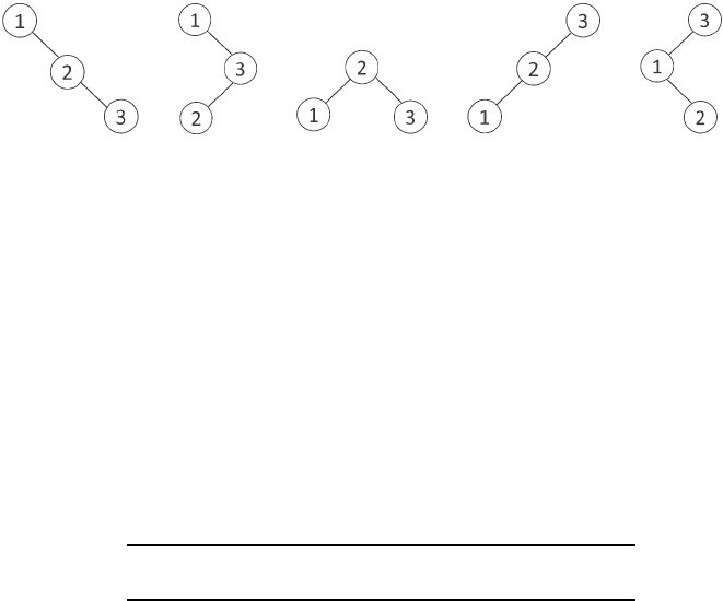
Among these six permutations, < 2, 3, 1 > is not stack sortable as shown in Section 15.4.

Thus, ﬁve permutations are stack sortable. Next, consider binary search trees that store the

three numbers.

It is not possible to have < 2, 3, 1 > as the result of pre-order traversal of a binary

search tree that stores 1, 2, and 3. This is not a coincidence. Suppose s(n) is the number

of possible stack-sortable permutations of 1, 2, 3, ..., n. It turns out s(n) is the Catalan

334 Intermediate C Programming

(a) (b) (c) (d) (e)

FIGURE 20.13: Five diﬀerent shapes for the pre-order traversals of binary search trees

storing 1, 2, and 3. (a) < 1, 2, 3 >, (b) < 1, 3, 2 >, (c) < 2, 1, 3 >, (d) < 3, 2, 1 >, (e)

< 3, 1, 2 >.

numbers as well. As illustrated by the example above, s(n) ≤ n! because there are n! possible

permutations of 1, 2,..., n. If n > 2, s(n) must be smaller than n!. We have already seen

that s(3) = 5 ≤ 3! = 6

Below is a proof that s(n) deﬁnes the sequence of Catalan numbers. Suppose a se-

quence of numbers < a

, a

, ...a

> is a particular permutation of 1, 2, ..., n and the

sequence is stack-sortable. Any preﬁx < a

, a

, ...a

>, k < n must be stack-sortable.

Suppose a

(1 ≤ i ≤ n) is n (the largest number in the entire sequence). Then the sequence

< a

, a

, ...a

> can be divided into three parts:

< a

, a

, ..., a

i−1

> a

= n < a

i+1

, a

i+2

, ..., a

What is the condition that makes a sequence stack-sortable? Section 15.4 explained

that max(a

, a

, ..., a

i−1

) must be smaller than min(a

i+1

, a

i+2

, ..., a

). Therefore, the ﬁrst

sequence must be a permutation of 1, 2, ..., i − 1 and the second sequence must be a

permutation of i, i + 1, ..., n − 1. Moreover, the two sequences < a

, a

, ..., a

i−1

> and

< a

i+1

, a

i+2

, ..., a

> must also be stack-sortable; otherwise, the entire sequence cannot be

stack-sortable. Therefore the entire sequence includes two stack-sortable sequences divided

by a

= n. By deﬁnition, there are s(i − 1) stack-sortable permutations of 1, 2, 3, ..., i − 1.

There are s(n −i) stack-sortable permutations of i, ..., n −1. The permutations in these two

sequences are independent so there are s(i − 1) × s(n − i) possible permutations of the two

sequences. The value of i is between 1 and n. When i is 1, the ﬁrst value in the sequence is

n and this corresponds to the tree in which the root has no left child. When i is n, the last

value is n and this corresponds to the tree in which the root has no right child. Thus, the

total number of stack-sortable permutations is:

s(n) =

i=1

s(i − 1) × s(n − i) =

n−1

i=0

s(i) × s(n − i − 1). (20.2)

This is the Catalan number.

Previous Chapter

20. Binary Search Trees (3/4)

Next Chapter

21. Parallel Programming Using Threads (1/5)

Table of Contents for Intermediate C Programming

Table of Contents for
Intermediate C Programming