Table of Contents for
Understanding Compression
 Understanding Compression
Published by
O'Reilly Media, Inc., 2016
Understanding Compression
Published by
O'Reilly Media, Inc., 2016
- Cover
- nav
- Understanding Compression
- Understanding Compression
- section
- Foreword
- Preface
- 1. Let’s Not Be Boring
- 2. Do Not Skip This Chapter
- 3. Breaking Entropy
- 4. Variable-Length Codes
- 5. Statistical Encoding
- 6. Adaptive Statistical Encoding
- 7. Dictionary Transforms
- 8. Contextual Data Transforms
- 9. Data Modeling
- 10. Switching Gears
- 11. Evaluating Compression
- 12. Compressing Image Data Types
- 13. Serialized Data
- 14. Lossy Data Compression
- 15. Making the World a Little Smaller
- Glossary of Compression Words
- Index
- About the Authors
- Colophon
Chapter 9. Data Modeling
Anyone who’s played the game “telephone” knows how important context is to the human brain. The words “cup” and “cop” taken by themselves are pretty likely to occur equally in most situations. However, if it’s a loud party, and you hear a word that you believe is either “cup” or “cop,” your brain will use the previous context to decide which one it was. For example, if your new friend said, “Wash the,” the next word is most likely “cup.” However, if they said, “Run from the”, it might be “cop.”1
This is the basic concept behind multicontext encoders. They take into account the last few observed symbols in order to identify the ideal number of bits for encoding the current symbol.
Perhaps a more concrete example is how symbol pairs influence the probability of subsequent letters in the English language.
For example, in “typical” English text, we expect to see the letter “h” about 5% of the time, on average. However, if the current symbol is a letter “t”, there is a high probability, actually about 30%, that the next symbol will be “h”, because the pair “th” is common in English. Similarly, the letter “u” has a general probability of about 2%. When a “q” is encountered, however, the probability is more than 99% that the next letter will be a “u”. In this case, the current symbol “q” predicts that the next letter will be “u”, and thus can use fewer bits assigned to it. This type of adjacency, based on statistical observance, has also dubbed this group of encoders “predictive”, which you’ll most likely see as the “proper” term in most official compression literature.2
This group can also be considered the “on-steroids” version of statistical compressors. They combine adaptive models (Chapter 3) and multiple symbol-to-codeword tables (Chapter 2) to produce the smallest codeword possible for the current symbol, based on previously observed symbols.
But this isn’t a new concept. It turns out that it was first presented back in the 1700s3 as one of the most powerful statistical computations to date.
The Chains of Markov
Markov chains are interesting creatures. Here’s the super-confusing technical definition:
A Markov chain is a discrete stochastic process in which the future depends only on the present and not on past history.
Given this definition, suppose for instance that we want to know the probability that a student will get an A in their math class in the fourth year of high school, and they have completed their third year. In general, we might expect that such a prediction will depend upon what grades they got in their first, second, and third years. However, if only the third (current) year had any bearing, and the grades in the previous two years could be ignored, this would be a Markov process.
Let’s work out a more detailed example.
You’ve just completed the most awesome 104 days of summer vacation of all time. As a post-mortem,4 you’ve decided to analyze how things went. You also decided to break down the analysis by days of the week. You found that on Mondays for the summer, there was a 50/50 split between activities, as shown here:
| Day | Activity | Probability |
|---|---|---|
|
Monday |
Spelunking |
50% |
|
Monday |
Bocce Ball |
50% |
You could describe this revelation in the following terms:
Given that today is Monday, there’s a 50/50 probability that we’ll either do spelunking, or bocce ball.
You find Tuesday has a more varied analysis.
| Day | Activity | Probability |
|---|---|---|
|
Tuesday |
Lounging at the pool |
10% |
|
Tuesday |
Sock hopa |
20% |
|
Tuesday |
Mowing lawns |
30% |
|
Tuesday |
Spelunking |
40% |
a It’s a Thing. Or rather, it used to be a Really Big Thing. | ||
Tuesday has a similar form, in that you could say, “If today is Tuesday, Sock Hop has a 20% chance of being our activity.”
Effectively, this is what we call a “second-order context.” We take two pieces of data and use them to define the probability of an activity. The day of the week acts as our “first order” or “context-1” data, the activity responds as the “second order” or “context-2” data, and the result is our percentage probability.
So, let’s try a third-order context:
| Day | First activity | Second activity | Probability of second activity |
|---|---|---|---|
|
Monday |
Bocce Ball |
Pedicures |
5% |
|
Monday |
Bocce Ball |
Smoothies |
95% |
|
Monday |
Spelunking |
SFHTML5 meetup |
50% |
|
Monday |
Spelunking |
Pizza |
25% |
|
Monday |
Spelunking |
Sewing class |
25% |
This example is a little more complex. Basically, “Given that today is Monday, AND we just did Bocce Ball, there’s a 25% chance we’re going to get some pizza.”
Each context describes a transition between states, to some known depth.
You could visualize this as a tree (Figure 9-1), where each node is an activity, and each transition has a probability.
Figure 9-1. A tree diagram of how a Markov chain would work
Markov and Compression
The concept of Markov chains fits nicely into our existing models because we can view statistical encoders as single-context Markov chains. Given one table of probability for the symbols of a stream, we assign codewords accordingly.
A second-context Markov chain could be created by adding a symbol-to-codeword table for each preceding symbol, such as that illustrated in Figure 9-2. Let’s see how this works.
Figure 9-2. A second-order or 2-context Markov chain uses a tree of symbol tables, as could be built for our summer vacation example.
Given the graph in Figure 9-2, to encode “Monday, Spelunking; Tuesday, Pool” we’d produce 0 1 10 1110 for a total of 8 bits. In contrast, if we were to enumerate each of the 10 states, we’d end up with something along the lines of 12+ bits to encode the same data.
From a technical standpoint, creating Markov chains for compression follows many of the rules we covered in adaptive statistical encoding (see Chapter 2); that is, reading in a symbol, dynamically updating a frequency table, and so on.
Encoding
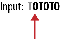
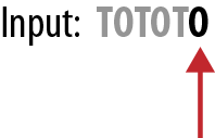
For example, let’s create a Markov chain for the string “TOTOTO”.
-
We begin by creating a context-1 table containing the <literal> symbol only at 100% probability.
Context-1 (overall probability of symbol)
Symbol
Frequency
Codeword
<literal>
100%
0
-
We read our first symbol, which is “T” and a new symbol.
-
We update the context-1 table to include “T” and adjust probabilities.
Context-1
Symbol
Frequency
Codeword
T
50%
1
<literal>
50%
0
-
We output <literal> and “T”.
Stream: 0 T
-
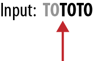
We read the next symbol from the stream, which is “O” and a new symbol.
-
We update context-1 to include “O” and updated probabilities.
-
We adjust the codewords to account for all symbols and satisfy the prefix property.
Context-1
Symbol
Frequency
Codeword
T
33%
0001
O
33%
001
<literal>
33%
01
-
We output <literal> and “O”.
Stream: 0 T 01 O
-
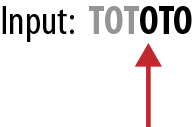
We read the next symbol from the stream, which is “T” and already in context-1.
-
We update context-1 to reflect the changed probabilities.
-
We swap the codewords so that the shortest one is for the symbol with the highest probability.
Context-1
Symbol
Frequency
Codeword
T
50%
01
O
25%
001
<literal>
25%
0001
-
We output the codeword for “T” to the stream, which is 01.
Stream: 0 T 01 O 01
-
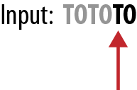
We read the next symbol from the stream, which is “O”.
-
We update the context-1 probabilities and leave our codewords unchanged.
Context-1
Symbol
Frequency
Codeword
T
40%
01
O
40%
001
<literal>
20%
0001
-
We output 001 to the stream.
Stream: 0 T 01 O 01 001
-
We can now create the second link in our Markov chain by starting a second symbol-to-codeword table that represents the characters following a “T” value.
Context-2, following “T” probabilities
Symbol
Frequency
Codeword
O
50%
0
<literal>
50%
1
-
We read the next symbol from the stream, which is another “T”.
-
We update the context-1 probabilities and leave the codewords unchanged. Context-2 for “following T” does not change.
Context-1
Symbol
Frequency
Codeword
T
33%
01
O
33%
001
<literal>
33%
0001
-
We output 01.
Stream: 0 T 01 O 01 001 01
-
We can now build a context-2 table for symbols following “O”.
Context-2, following O probabilities
Symbol
Frequency
Codeword
T
100%
0
-
We read the final symbol, which is “O”.
-
We can now take advantage of the context-2 table created for “following T” and output 0 as our final symbol.
Final stream: 0 T 01 O 01 001 01 0
And voilá, compression!
Decoding
To prove that this is reversible and works, let’s decode our stream:
-
Read 0. We know this is the literal symbol, so we build our context-1 table with it (100%).
0 T 01 O 01 001 01 0
-
Read “T”. Literal. Add this to context-1 and adjust probabilities (50/50).
Output: T
-
Read “01”. According to context-1, this announces another literal.
-
Read “O”. Update context-1 (33/33/33).
Output: O
-
Read “01”. According to context-1, this is “T”. Update context-1 (50/25/25).
Output: T
-
Read “001”. According to context-1, this is “O”. Update context-1 (40/40/20).
Output: O
-
Build context-2 for following “T”.
-
Read “01”, which is “T”. Update context-1 (33/33/33).
Output: T
-
Build context-2 for following “O”.
-
Read “0”. Preceding context is “T”, looking 0 up in context-2 “following T”, we get “O”.
Output: O
And there you have it.
You can do the same thing with more symbols and longer strings, and as you can see, it gets pretty complex pretty fast.
Compression
For all that complexity, how do we win in terms of compression?
When applied to compression, Markov makes it possible for you to encode adjacent symbols with fewer bits.
Look at the two context-2 tables. They both contain 0, the shortest possible encoding. Because we are using the preceding symbol as disambiguation context, we can use the same short VLC twice, thus saving bits. Another way of saying this is that each context has its own VLC space, and thus we can use the same VLC.
After we have more symbols and longer input streams, we can build up multiple contexts. Using the English language as an example, T could be a context, with H following, and TH could be another context, with E, I, U, O, and A following.
Although U on its own has a frequency of 2.7%, which would assign it a pretty long code, in the particular context of “following Q”, it would get a much shorter code.
And this makes Markov chains exceptionally powerful.
Practical Implementations
It’s worth pointing out that no one really uses Markov chains for compression. At least not in the way just described.
Consider a worst-case—but not implausible—scenario, in which you have an 8-context chain.
This means that for each node, you’re going to end up with 256 other child nodes, 8 deep. This means that you will need 2568 (two-hundred-fifty-six-to-the-power-of-eight!) or 16 exabytes of memory6 to represent your tables. Which is crazy, even by modern computing standards.7 As such, various derivative algorithms have been created that are just a little more practical about memory and performance than a general Markov chain. The most notable ones are prediction by partial matching and Context Mixing, which we are going to take a look at next.
Prediction by Partial Matching
A practical implementation of Markov is all about understanding memory and quickly being able to encode the most optimal chain. A memory- and computationally efficient approach to Markov chains was created by John Cleary and Ian Witten back in 1984,8 called prediction by partial matching (PPM). Much like Markov chains, PPM uses an N-symbol context to determine the most efficient way to encode the N + 1th symbol.
Whereas a simple Markov implementation works in a forward manner by reading the current symbol and seeing if it’s a continuation of the existing chain, PPM works in reverse. Given the current symbol in the input stream, PPM scans back N symbols and determines the probability of the current symbol from the N previous symbol context. If the current symbol has a zero probability with the N-context, PPN will try an N - 1 context. If no matches are found in any context, a fixed prediction is made.
For example:
-
Suppose that the word “HERE” has been seen several times while compressing an input stream, so context has been established.
-
Somewhere later, the encoder starts compressing “THERE” and is currently compressing the R symbol.
-
In a 3-symbol context, the previous symbols of R are “THE”.
-
However, this encoder has never seen “THER”, only “THE ” (with a space).
-
As such, the current R has “zero probability”. (That is, R hasn’t been encountered before, given the previous 3–symbol context.)
-
At this point, PPM would try a 2-symbol context, attempting to match “HER” as a chain.
-
This results in a success because “HERE” has been seen many times before, which among others, created a 2-context for “HE”.
-
Thus “R” has a “nonzero probability” based on the 2-context chain “HE.”
Here’s a more formal version:
-
The encoder reads the next symbol “S” from the input stream.
-
The encoder looks at the last N symbols read; that is, the order-N context.
-
Based on this input data that has been seen in the past, the encoder determines the probability P that “S” will appear following the particular context.
-
If the probability is zero, the encoder emits an escape token for the decoder so that the decoder can mirror the process.9
-
Then, the encoder repeats from step 2 with N = N – 1, until the probability is nonzero, or it runs out of symbols.
-
If the encoder runs out of symbol, a fixed (e.g., based on character frequency) probability is assigned.
-
The encoder then invokes a statistical encoder to encode “S” with probability P.
The Search Trie
The main problem with any practical implementation of PPM has to do with the creation of a data structure where all contexts (0 through N) of every symbol read from the input stream are stored and can be located quickly. In simplistic cases, this can be implemented with a special tree data structure called a trie,10 for which each branch represents a context.
For example, let’s build a PPM trie for the string “ABAC”, with a maximum11 allowed context of 2, as depicted in Figure 9-3.
-
Reading in the first value, “A”, appends a new node [A,1] to the root of the tree. This represents that “A” has been seen 1 time so far at context 1. (Children of the root node are context 1, grandchildren are context 2, and so on).
-
Reading the second value, “B”, adds two nodes to the tree.
-
First, it adds an order-1 context node, [B,1]. This is useful in the case where “B” is the start of its own context chain.
-
Second, it adds an order-2 context node [B,1] under the [A,1] node. This is to represent the chain “AB” that we’ve read through the input stream so far.
-
-
Reading the next “A” value has a few tricks.
-
First, it updates the count value of the order-1 context node, (because “A” has already been encountered at that context).
-
Next, it adds an [A,1] node as a child of each [B,1] nodes. This represents both the order 1 and order 2 contexts of “BA” and “ABA”, respectively.
-
-
The final symbol, “C” follows a similar process, but with a small change.
-
We add the order-1 context node [C,1].
-
The next step would be to add 4-order [C,1] nodes to all 3-order [A,*] nodes. You can see that on the lefthand side, this is completed fine with the [B,1]->[A,1] chain. However, on the right side, adding the new node would violate our context height restriction. So, we append nothing.
-
As a final step, we have a valid [A,1] node at order-1, and add a [C,1] node as a child there.
-
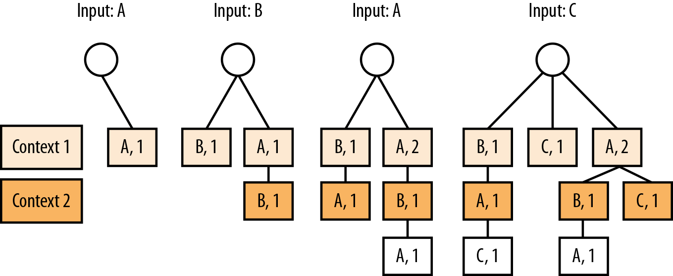
Figure 9-3. Building a PPM trie with an N-context of 2. Each level of the tree represents a context. The children of the root are the first-order context. The number next to the character denotes how many times that symbol has been encountered, at that context.
This trie is beneficial, in that we can quickly query the N-minus-X contexts, given a current state. For example, given a symbol “C”, our 2-order context is “BA”, our 1-order context is “A”. This fits perfectly because it represents a sliding window of the previous one and two symbols from “C” in the “ABAC” string we encoded.
We can use this trie to represent all of the following substrings of the input, given a 2-context limit (Figure 9-4): B, BA, BAC, C, A, AB, AC, and ABA.
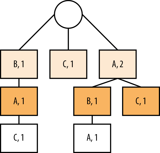
Figure 9-4. Strings represented by this trie: B, BA, BAC, C, A, AB, AC, and ABA.
Compressing a Symbol
In addition to providing efficient storage and fetching of substrings, the trie structure also contains counts per level. A statistical encoder can use these to build probability tables and assign encodings for each symbol, as shown in Figure 9-5.
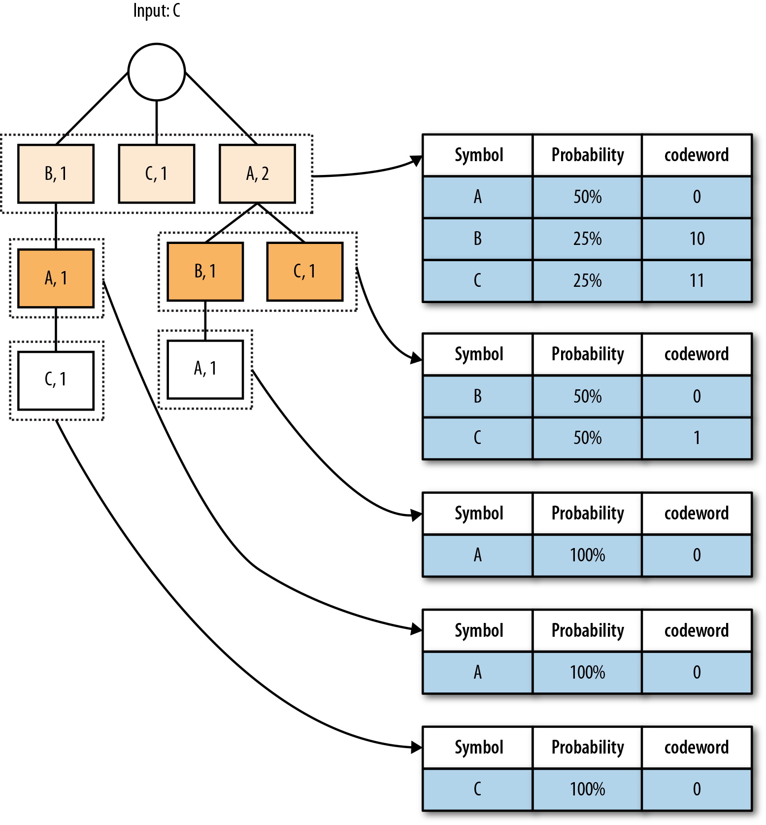
Figure 9-5. The PPM trie, and an example of the symbol-to-codeword tables you could use for encoding.
Effectively, given a level, we only need to consider the siblings at this level and normalize their values to arrive at probabilities. For example, the context-1 counts of [B,1], [C,1], and [A,2] would represent probabilities of 25%, 25%, and 50%, respectively.
Also, note that because we can use 1-bit encodings in context-2, for every symbol encountered in context, we save 1 bit, for potentially substantial savings.
You can implement this in a straightforward fashion as a modification to the data structures we covered in Chapter 3.
Choosing a Sensible N Value
So what is the value of N supposed to be? PPM selects a value N and tries to make matches based on that context length. If no match is found, a shorter context length is chosen. As such, it seems that a long context (large value of N) would result in the best prediction. However most PPM implementations skew toward an N value of 5 or 6, trading off memory, processing speed, and compression ratio.
There are variants of PPM, such as PPM*, which try to extend the value of N and make it exceptionally large. You can do this with a new type of trie data structure, and significantly more computational resources than PPM. This usually results in about 6% better savings than straight-up PPM.
Dealing with Unknown Symbols
Much of the work in optimizing a PPM model is handling inputs that have not already occurred in the input stream. The obvious way to handle them is to create a “never-seen” symbol which triggers the escape sequence. But what probability should be assigned to a symbol that has never been seen? This is called the zero-frequency problem.
One variant of PPM uses the Laplace estimator, which assigns the “never-seen” symbol a fixed pseudo-count of one. A variant called PPMD increments the pseudo-count of the “never-seen” symbol every time the “never-seen” symbol is used. (In other words, PPMD estimates the probability of a new symbol as the ratio of the number of unique symbols to the total number of symbols observed.)
PPMZ presents one of the more interesting variants. It starts in the same way as PPM* does, by trying to match a N-context probability for the current symbol. However, if a probability isn’t found, it switches to a separate algorithm called a Local-Order-Estimator and uses the basic PPM model, with a completely separate predictor.
Context Mixing
Trying to improve PPM algorithms has led to the PAQ series of data compression algorithms—in particular, work in the PPMZ area, where multiple types of context tries are used, based on how a symbol responds to matching.
This concept evolved over time into context missing; that is, using two or more statistical models of the data in order to determine the optimal encoding for a given symbol. For example, using a statistical model of how often you visit “The Gym” against all your regular activities (like rescuing kittens), and another statistical model of probability of visiting “The Gym” within 12 hours of eating too much spaghetti. Given the question of “What’s the probability that I will go to the gym right now?”, each model will yield a different probability. Because there is a 20% chance that you go to the gym generally, and because it’s been six hours since indulging in Italian cuisine, you’re 50% likely to go to the gym right now. The combination of those probabilities is what context mixing is all about.
Context mixing brings two interesting questions to the table with respect to data compression:
-
What types of models should you use on the data?
-
How should you combine those models?
Types of Models
As we discussed earlier, adjacency is a very important topic to data compression. Algorithms such as LZ, RLE, delta, and BWT all work from the assumption that the adjacency of our data has something to do with the optimal way to encode it.
When introducing Markov, it’s easy to present it in this same light. Creating an adjacency-based context is easy to do (“if A follows B”, etc.). But in reality, this is just one way to create a contextual correlation between symbols. For instance, you might create a context as all values in an even index, or context might be derived from values which are clustered around a certain numerical range. Basically, adjacency and locality are the simplest forms of contextuality, but by no means are they the only ones.
With this mentality, it makes logical sense that there might be other signals in the data stream that could help us identify the right way to encode the current symbol, signals that have nothing to do with context or adjacency. Identifying and describing the relationships between symbols is what we call models. By modeling the data, we understand more about the various attributes it contains, and can we better describe the current symbol.
In reality, models can be anything and can change depending on the type of data you have.
For example, images care a lot about two-dimensional locality; that is, a pixel color generally has something to do with the adjacent colors above, below, and on each side of it, and we can take advantage of that for compression. This model doesn’t work for text though. There’s generally no observance that a character has any proper relation to one below or above it.12
In programming, after compiling your high-level instructions into bytecode, there’s a completely separate model. A single byte can describe an instruction, followed by a set of variable-length bytes that describe the input to that function. Because code tends to have common patterns, you could model that if you see a “Jump to this instruction” command, there’s most likely going to be a “push the variables onto the call stack” command around here somewhere, as well. So in this case, it’s not important to note the adjacent bytes, but the commands themselves.
Music is a completely different beast. You could create models to represent the bass line, or guitar riffs, and take into account the lengths of courses or bridges that are involved.
The point here is that there’s thousands of different ways to model your data if you just know enough about it to ask the right questions. So the problem becomes more difficult in some cases, because now, we’re not talking about generic algorithms, but more asking the question, “Do you understand enough about your data to model it properly?”
One of the pioneering compressors in the context mixing space, PAQ, includes the following models:
-
N-grams. The context is the last N bytes before the predicted symbol (as in PPM).
-
Whole-word n-grams, ignoring case and nonalphabetic characters (useful in text files).
-
“Sparse” contexts. For example, the second and fourth bytes preceding the predicted symbol (useful in some binary formats).
-
“Analog” contexts, consisting of the high-order bits of previous 8- or 16-bit words (useful for multimedia files).
-
Two-dimensional contexts (useful for images, tables, and spreadsheets). The row length is determined by finding the stride length of repeating byte patterns.
-
Specialized models that are only active when a particular file type is detected, such as x86 executables, or BMP, TIFF, or JPEG images.
And PAQ is no joke. It’s constantly at the top of the Large Text Compression benchmark, and one of the newer versions, ZPAQ, attained second place in a contest compressing human DNA.
Types of Mixing
Just off the cuff, how would you mix two given values? Average them? Add them together? Maybe weigh them differently based upon user preference or prior input? And these questions become more complex as you start using multiple models. After you have a set of 50 inputs, how do you combine models to pick the best compression?
Thankfully, statistics have mostly solved this problem for us. There are two types of approaches to mixing the outputs from different models together.
Linear mixing is a process of using the weighted average of the predictions, where the value comes from the weight of the evidence.
In our previous example, we were trying to figure out the probability of you going to the gym given how often you go to the gym, and how often you eat pasta. Now, these two values have a different evidence weight, in that one might be proving a more reliable value due to more tests/samples taken. For example, if you’re considering how pasta influences your gym attendance at a lifetime level, it would have more sample data and thus be a more reliable form of predictor than, say, your frequency of going to the gym in the last week.13 As such, we give one more weight in the mixed model due to it having more evidence.
Logistic mixing, on the other hand, is crazy.
You see, with linear mixing, there’s really no feedback loop to indicate to you whether the weight you assigned to a model was correct toward predicting how to compress this data. So, if your input stream changes, and the weighting of your models stays the same, you can end up bloating your output stream.
To address this, logistic mixing uses a neural network (artificial intelligence!) to update weights and reassign them based upon what models have given the most accurate predictions in the past. The trick here is with correcting the current weightings. Suppose that the current weight selects model A to encode this symbol in 12 bits. But model B would have been the correct choice, with an 8-bit encoding. The encoder outputs the 12 bits and then updates its weights so that when all of these models produce these same values next time, model B has a higher chance of being chosen.
The only downside to this is the massive amount of memory and running time it takes to compress the data. If you look at ZPAQ on the LTCB, it took 14 GB of memory to compress a 1 GB file. All that modeling data has to go somewhere, right?
The Next Big Thing?
Context mixing shines a light on the future of data compression. Basically, with unlimited memory and running time, combined with enough modeling knowledge of the data, optimal compression is a solved problem. This might be the next big solution to data compression at a cloud-computing level. Companies that have tons of compute resources and time to spend on them, could be able to aggressively compress data, given that their data-science team has properly identified all the models for it.
But this hasn’t yet made its way to the consumer market. The high overhead of memory and runtime make context mixing improbable for mobile devices (at the time of writing this book). But the reality is that it’s a completely different data target. If you’re only dealing with 1 MB to 50 MB of data, the results of compressing using context modeling are pretty similar to a lot of other algorithms out there. It’s when your data is large, complex, and ever-changing that context mixing begins to shine.
So, this goes back to the same thing again: there’s no silver bullet when it comes to compression. Each data set needs a unique thought process and analysis on how to define and approach the information. Even context modeling, which is built to adapt to the data, still relies on humans creating models for the information.
Which means there’s one thing for certain: data compression is far from a solved problem, and there is so much more awesomeness left to discover there.
1 But it is the Internet, so there could be a place where you’re washing cops and running from cups... *shrug*
2 Note that in every common piece of compression literature, these are called “Prediction” coders. We really don’t like this terminology, because “predict” implies “can be wrong.” Which seems to run counterintuitive to compression; if your encoding or decoding is wrong in predicting what symbol is next, you end up with a broken compression system. Instead, we prefer to refer to these algorithms as multicontext, in that they weave together multiple symbols and statistical tables/models in order to identify the least number of bits needed to encode the next symbol.
3 Decision support systems have a long history going back to Pascal.
4 Evaluation of summer vacation is a totally common thing to do for people that read books on compression.
5 Actually, this is the one paragraph in the book where the coauthors were not in agreement. Because, obviously, it would be cute kittens who saved the day.
6 Or 17,179,869,184 GB.
7 This sentence was written in 2015, when dual-core mobile devices ruled the earth like vengeful gods.
8 J. Cleary, and I. Witten, “Data Compression Using Adaptive Coding and Partial String Matching,” IEEE Transactions on Communications 21:4 (1984): 390–402.
9 Yes, you’re absolutely correct. This means that if a symbol has never been encountered before, PPM can emit N “escape codes” to the stream before the final literal symbol. Most of the differences between variants of this algorithm (PPMA and PPMB, PPMC, PPMP and PPMX) have to do with how they handle nuances in this escape-code process.
10 This is the proper spelling: stick with us and find out why.
11 Limiting the number of context levels is one way of controlling complexity.
12 ...unless you are compressing word games or some very wacky poetry.
13 We are totally going to the gym next week. We hear there’s a new spin class we should check out.