Table of Contents for
Understanding Compression
 Understanding Compression
Published by
O'Reilly Media, Inc., 2016
Understanding Compression
Published by
O'Reilly Media, Inc., 2016
- Cover
- nav
- Understanding Compression
- Understanding Compression
- section
- Foreword
- Preface
- 1. Let’s Not Be Boring
- 2. Do Not Skip This Chapter
- 3. Breaking Entropy
- 4. Variable-Length Codes
- 5. Statistical Encoding
- 6. Adaptive Statistical Encoding
- 7. Dictionary Transforms
- 8. Contextual Data Transforms
- 9. Data Modeling
- 10. Switching Gears
- 11. Evaluating Compression
- 12. Compressing Image Data Types
- 13. Serialized Data
- 14. Lossy Data Compression
- 15. Making the World a Little Smaller
- Glossary of Compression Words
- Index
- About the Authors
- Colophon
Chapter 6. Adaptive Statistical Encoding
Locality Matters for Entropy
All the statistical encoders mentioned in Chapter 5 require an initial pass through the data to compute probabilities before encoding can start. This leaves us with a few shortcomings: you always need to do an extra pass through the data to calculate the probabilities, and after you have calculated the probabilities for the entire data set, you are stuck with those numbers. Neither of those is a problem for relatively small data sets.
However, the larger the size of the data set that you’re compressing, the more bloated your statistical encoding will be with respect to entropy. This is because different subsections of the data set will have different probability characteristics. And if you’re dealing with streaming data—a video or audio stream, for example—there’s no “end” to the data set, so you just can’t “take two passes.”
These concepts, then, will apply to streaming data, but let’s look at them in the context of a relatively simple example data set. The first third of your stream might contain an excessive number of Q’s, whereas the last two thirds might have exactly none. The probability tables for your statistical encoder would not account for this locality. If the symbol Q has a probability of 0.01, it is expected to appear more or less evenly along the entirety of the stream; that is, about every 0.01th value would be Q.
This is not how real data works. There’s always some sort of locality-dependent skewing1 that bundles symbols, thoughts, or words together in subsections of your data set.
As a consequence, the probability information that the statistical encoders are built on creates codes that are bloated with respect to entropy: they don’t take into account local shifts in the statistics. If, for example, you broke up a stream into N chunks and compressed each one individually, you might end up with a smaller output than by compressing the entire input as one (if there’s lots of locality-dependent skewing2).
Let’s consider a simple example data set:
AAAAAAAAAAAAAAAAAAABBBBBBBBBBBBBBCDEFGHIJKLMNOPQRSTUVWXYZ
This stream has an entropy of ~3.48, suggesting that we should, on average, use about 3.48 bits per symbol, and expect a final encoded size of 198.36 bits. The Huffman-encoded version of this set is about 202 bits, which puts us at about 3.54 bits per symbol,3 which is not too shabby.
But let’s be honest here. We can do better than that. We can plainly see that the first half of the stream is made up of only two characters, highly repeated. In reality, we’d love to find a way to split the stream, so that we could get better encoding for the first half of the stream. Wouldn’t it be great, if instead of creating one variable-length code (VLC) for the entire stream, we could break it in half, and assign the first half 1 bit per symbol, and the second half 5 bits per symbol? The net result would be 122 bits, giving us 2.1 bits per symbol. (And just to point this out, this has us beating Shannon. In a blowout.)
This leads us to a very important place in the compression world, the concept that locality matters.4 As data is created in a linear fashion, there’s a high probability that parts of the stream will have characteristics that are completely different from other parts of the stream.
The real challenge of implementing this type of optimization is in how to optimally divide the stream. Scanning ahead as we go, and trying to find the right segments, will only lead you to madness and something that feels like an NP-complete problem. So, instead of trying to scan ahead and find the right split points as we are encoding, we instead allow our statistical encoders to “reset” themselves.
This process is pretty simple in concept: As we’re encoding our stream, if the variance between the “expected” entropy and the “actual encoded bits” begins to diverge by a significant amount, the encoder resets the probability tables, and then continues using the reset tables.
This ability of adapting to the locality of the entropy of a stream is often called a “dynamic” or “adaptive” variant of a statistical encoder. And these variants make up the majority of all important, high-performance, high-compression algorithms for most media streams, such as images, video, and audio.
Adaptive VLC Encoding
Let’s look at perhaps one of the simplest versions of an adaptive algorithm, just to understand the basic workings.
Typically, there are three stages to statistical compression:5
-
Walk through the stream and calculate probabilities.
-
Assign variable-length codes to symbols based on their probability.
-
Walk through the stream again and output the appropriate codewords.
Basically, you do two passes through the data stream and have one VLC set for the entire set of data. The issue here is the static nature of the VLC table.
Now the adaptive version of this process collapses these three steps into a single, very complex, pass through the data set. The key lies in our symbol-to-codeword table not being set in stone; rather, it can update as it encounters symbols.
Note
The trick to adaptive statistical encoding has to do with not having a set-in-stone VLC table. Instead, the VLC is constructed on the fly as symbols are encountered. The dynamic nature of this process lets us do other stuff to the table as we see fit; like, reset it.
Dynamically Building a VLC Table
Dynamically building your VLC table follows this pattern:
As the encoder processes the data stream, for each symbol it encounters, it asks the following:
-
Have we encountered this symbol yet?
-
If so, then output its currently assigned codeword, and update the probabilities.
-
If not, then do something special. (We will get to this part in a bit.)
-
So, with that in mind, suppose that as you begin processing your stream, you’ve been given some expected probabilities and symbols to start with. As such, you currently have a VLC table that looks like this:
| Symbol | Probability | Code |
|---|---|---|
|
A |
0.5 |
0 |
|
B |
0.4 |
10 |
|
C |
0.1 |
11 |
Now, let’s read the next symbol off the input stream, which happens to be the symbol B:
-
Output the currently assigned codeword for B, which is 10.
-
Update the probabilities table because B has just become a little bit more probable (and the other symbols a little bit less).
Symbol Updated probability Code A
0.45
0
B
0.45
10
C
0.1
11
-
The next symbol is a B again, so we output a 10 again, and update our probabilities.
Symbol Updated probability Updated code A
0.4
10
B
0.5
0
C
0.1
11
Notice the important thing that happened here. Because B has become the most probable symbol in our stream, it is now assigned the shortest codeword. If the next symbol we read is another B, the output will now be 0 instead of the previous 10.
By dynamically updating the probabilities of symbols as we come across them, we can adjust the sizes of the codewords that are assigned to them, if necessary.
Decoding
Just to ensure that this actually works, let’s take a look at the decoding process.
Let’s begin again with our setup frequencies6 and the following VLC table:
| Symbol | Probability | Code |
|---|---|---|
|
A |
0.45 |
0 |
|
B |
0.45 |
10 |
|
C |
0.1 |
11 |
We take the next bits of the input stream, see 10, and output B. We also update our probability table, because we’ve seen another B.
| Symbol | Updated probability | Updated code |
|---|---|---|
|
A |
0.4 |
10 |
|
B |
0.5 |
0 |
|
C |
0.1 |
11 |
Lo and behold, the table is evolving in the same way as when we were encoding.
Everything works!
And, as long as our decoder is updating its symbol table in the same fashion as the encoder, the two will always be in synchronization.
Check it out:
- Encoding
-
-
Read symbol from input stream.
-
Output that symbol’s codeword to the output stream.
-
Update the symbol table probabilities and regenerate codewords.
-
- Decoding
-
-
Read the codeword from the input stream.
-
Output that codeword’s symbol to the output stream.
-
Update the symbol table probabilities and regenerate codewords.
-
This is the basic process of how adaptive statistical encoding works. The encoder and decoder are both dynamically updating their probability tables for symbols, which affects the compression, usually in a positive way.
Literals
But now we run into two challenges:
-
What does our VLC table look like at the start, before we have encoded anything?
-
What happens during decoding, when we read in a symbol that doesn’t yet exist in our VLC table?
They are actually variations on the same problem, and the answer is: literal tokens.
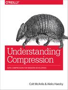
A literal token is a unique “fake” symbol that the encoder and decoder use to signal that it’s time to read/write a symbol from the literal stream. The literal stream is a second stream that only holds literal values; that is, the actual, encoded symbols in the order in which they are encountered first in the data stream.
For example, for the datastream “AAAAABCABC” the literal stream would be “LITERAL/A/B/C,” and the encoded stream might look like 00 1010 01 00 00 00 01 1011 01 1100 00 10 11, as shown in Figure 6-1.
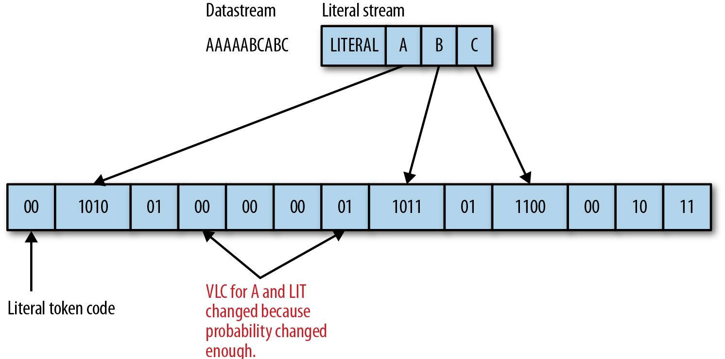
Figure 6-1. Example illustrating how literal tokens, reading from the literal stream, and changed probabilities appear in an encoded data stream.
During encoding, when the encoder reads a symbol it hasn’t come across before, it does two things:
-
It emits the LITERAL codeword to the output bit stream.
-
It appends the new symbol to the literal stream.
And during decoding, when the decoder reads a LITERAL codeword, it does these two things:
-
It reads the next literal from the literal stream.
-
It adds that literal to the output and updates its VLC table.
Let’s take a look at an example.
When we start encoding our stream, we haven’t seen any symbols yet, so we know that for the very first symbol we read, we’ll need to emit a literal. It’s our only option. As such, we begin our VLC table with LITERAL being the only symbol present, with 100% probability, and a single bit codeword.
| Symbol | Probability | Code |
|---|---|---|
|
<LITERAL> |
1.0 |
00 |
When we encounter a new symbol from the input stream, we first output the VLC for the LITERAL codeword, followed by the bits for the new symbol. And just like before, we then update our table and probabilities accordingly.
| Symbol | Probability | Code |
|---|---|---|
|
<LITERAL> |
0.5 |
00 |
|
A |
0.5 |
01 |
Suppose that after that we read another A. And then we read B, another new symbol, and having arrived at <LITERAL> A A <LITERAL> B, our probabilities now are:
| Symbol | Probability | Code |
|---|---|---|
|
<LITERAL> |
0.4 |
01 |
|
A |
0.4 |
00 |
|
B |
0.2 |
10 |
So, for our input string AAAAABCABC, here is the complete algorithmic example. (You can refer back to Figure 6-1 for visual cues.)
The unencoded 4-bit values for our literals are:
A = 1010
B = 1011
C = 1100
Note that, for our VLC codes, we’re just using 00, 01, 10, 11 to keep the explanation simple.
-
Our VLC table contains LITERAL with a 1.0 probability, and its VLC is 00.
-
Read the first symbol, A.
-
The symbol is not in our table, so we must emit a literal token (which is 00) and then the value of A: 1010.
-
Add A to our VLC table and update it based upon frequency. Since A and LITERAL have both been seen once, their probability is 0.5 each, and we assign them the codes: LIT=00, A=01.
-
-
Read the next symbol, A.
-
Since A is in the table, emit its VLC (01).
-
Update the table. A is now the most dominant symbol, and thus the VLCs get reassigned: A=00, LIT=01.
-
-
Read the next symbol, A.
-
Emit A’s VLC (00) and update the probabilities in the table.
-
-
Read the next symbol, A.
-
Emit A’s VLC (00) and update the table.
-
-
Read the next symbol, A.
-
Emit A’s VLC (00) and update the table.
-
-
Read the next symbol, C.
-
C is not in our table, so emit a literal token (01) and then the value of C, which is 1100.
-
Add C to our VLC table, and update; A=00, LIT=01, B=10, C=11.
-
-
Read the next symbol, A.
-
Emit A’s VLC (00) and update the table.
-
-
Read the next symbol, B.
-
Emit B’s VLC (10) and update the table.
-
-
Read the next symbol, C.
-
Emit C’s VLC (11) and update the table.
-
And voilà, the resulting stream is: 00 1010 01 00 00 00 01 1011 01 1100 00 10 11 (see Figure 6-2.)
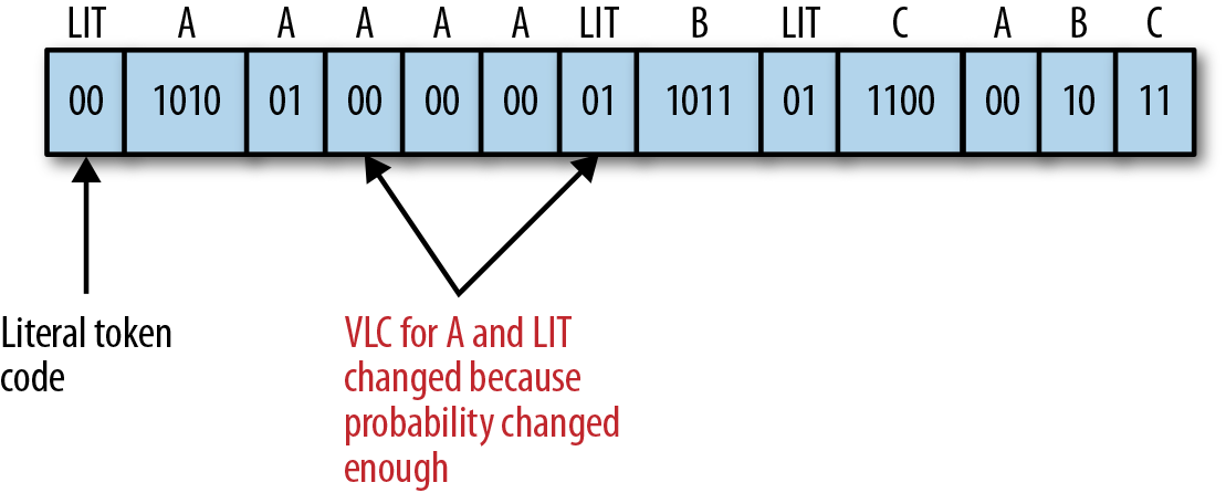
Figure 6-2. Final encoded stream.
Next, can you decode this by reversing the steps?
Resets
The real power of adaptive statistical encoding comes from being able to reset the stream when the output entropy gets out of hand.
Let’s take [AAABBBBBCCCCCC] and represent literals as their values in angle brackets, such as <A>.
As we encode this stream, we end up with the following:
<A>,0,0,<B>,1,1,1,0,<C>,11,11,11,11,0
Note that the last 0 for the last C is when the probabilities finally shifted to change the code for C. You can see how with more symbols, and more runs of symbols, the overall bits-per-symbol for output will suffer. It would have been ideal instead to somehow reset our VLC table when we got to C so that we could use 0 for all Cs for a better result and end up with something like this:
<A>,0,0,<B>,1,1,1,0,<C>, <RESET>0,0,0,0,0
As it turns out, we can employ the same tactic that we used with literals and create a <RESET> token, as shown in the example table that follows. Whenever the decoder encounters this token, it resets its symbol table and begins decoding afresh. The encoding and decoding algorithms work the same as before.
The <RESET> and <LITERAL> tokens stay in the symbol table (like any other symbol) and over time, become lower probabilities as they become less frequent.
Following is an example table showing that <RESET> and <LITERAL> tokens will eventually become lower-probability symbols.
| Symbol | Probability | Original interval |
|---|---|---|
|
<LITERAL> |
0.05 |
1110 |
|
<RESET> |
0.05 |
1111 |
|
A |
0.4 |
00 |
|
B |
0.3 |
10 |
|
C |
0.2 |
110 |
Knowing When to Reset
But how do you know when to emit a reset token?
To make the decision to reset, we need to do three things:
-
Choose a threshold for resetting; that is, at how many bits-per-symbol (BPS) we are going to pull the plug and start from scratch.
-
Measure roughly the average BPS that we have emitted to the output stream so far and compare that to our threshold.
-
Calculate the current entropy for the input stream we’ve read so far.
When the BPS for the output stream exceeds a chosen threshold, say, 5 bits greater than BPS, we can assume that the stream has significantly changed, and we should reset all our statistics.
Specifically, if we track the entropy for the input symbols, we’ll find that the number of bits in the output stream will generally be larger than that entropy value. Or, stated formally:
Entropy * numSymbolsSoFar > len(outputbits)
This is because we can’t represent fractional bits in modern hardware. Instead, we can divide the number of output bits by the number of input symbols to give us the “average output BPS,” as shown here:
aobp = len(outputbits)/numSymbolsSoFar
When we compare entropy to aopb, the result shows us how much the output stream is drifting from the estimated desired number of BPS.
When we drift past our threshold (abs(aopb-Entropy) > threshold), we should reset, because the output bitstream is getting too bloated.
Threshold isn’t a hard-and-fast rule and varies depending on the data stream/encoder. Each encoder that supports this type of reset has fine-tuned these parameters for the particular data it is designed to handle.
Using This in Practice
So, it’s worth pointing out that no one uses this simplified version of adaptive VLCs in any real capacity. The same problems with the static version of VLCs follow over to the streaming adaptation. Instead, most modern compressors have jumped entirely to using adaptive versions of Huffman and arithmetic coders that allow for dynamic probability table generation and updated codeword selection.
However, these last few sections were not in vain. The same concepts that power dynamic VLCs—that is, dynamic probability tables, resets, and literals—are all very much present in the adaptive Huffman and adaptive arithmetic coders.
Adaptive Arithmetic Coding
Arithmetic coding is quite easy to make adaptive. This is mostly due to the simplicity of the interaction between the coding step and the probability table. As long as the encoder and decoder agree about how to update the probabilities in the correct order, we can change these tables as we see fit.
Here is a very simple example. Our assumed probability table is as follows, so far:
| Symbol | Probability | Original interval |
|---|---|---|
|
R |
0.4 |
[0, 0.4) |
|
G |
0.5 |
[0.4, 0.9) |
|
B |
0.1 |
[0.9, 1.0) |
-
We read in the next input symbol; let’s assume that it’s the letter G.
-
We encode the symbol using the current probabilities.
-
We update the probability tables with the new information. (We are just going to assume values for the table that follows for this example because we didn’t define the preceding stream.)
-
We reassign the intervals.
| Symbol | Updated probability | Updated interval |
|---|---|---|
|
R |
0.3 |
[0.4,0.55) |
|
G |
0.6 |
[0.55, 0.85) |
|
B |
0.1 |
[0.85, 0.9) |
And here is how this plays out as a diagram:
The decoder works in the opposite way. Given the current probability, find the symbol that corresponds to the current numeric output value, update the tables, and reassign the intervals.
Adding literal and reset tokens works in the same way as adaptive VLC. You designate these tokens types as additional symbols, and adjust their weights accordingly.
Adaptive Huffman Coding
Making Huffman coding adaptive isn’t as straightforward as it was for arithmetic. This is mainly due to the complexity that arises when dealing with the Huffman tree data structure.
Consider the problem: to properly output a codeword, a full Huffman tree is required. A naive implementation would simply recompute the entire Huffman tree for each symbol that’s encountered. This would work, although at the cost of a huge amount of compute performance.
So, rather than rebuilding the entire tree each time, the adaptive Huffman version modifies the existing tree as symbols are being read and processed. Which is where things get a little crazy, because for each symbol read you must do the following:
-
Update the probabilities.
-
Shuffle and reorder a large number of nodes in the tree to keep them accurate with respect to the changing probabilities.
-
Stay compliant with the required structure of the Huffman tree.
The original versions of this adaptive Huffman method were developed in 1973 by Faller,7 and substantially improved by Knuth in 1985.8 But modern variants are all built on Vitter’s method, introduced in 1987.9 Refer to the papers referenced in the footnotes, if you’d like to dig into the specifics.
The Modern Choice
These dynamic adaptations have a few benefits over their static counterparts:
-
Ability to generate the symbol-to-codeword table rather than storing it explicitly in the stream. This can trade data-stream size for additional compute performance, but more important, this enables the next two benefits.
-
Ability to compress data as it arrives, rather than needing to process the set as a whole. This lets you process much larger data sets efficiently, and you don’t even need to know ahead of time how large your stream is going to be.
-
Ability to adapt to locality of information; that is, adjacency can influence code lengths. This can significantly improve the compression rate.
These three points are very important for modern statistical encoding. As the amount of data is growing, more and more of it is sent over the Internet, and increasingly, people consume data on mobile devices, which have limited storage and stingy data plans. As such, the majority of statistical encoders concern themselves with compressing images (WebP) and video (WebM, H.264).
What this means for you, however, is that for small data sets, the simplicity of static statistical encoders might work fine, and help you to achieve entropy with very low complexity. If you’re working on larger data sets, or multimedia ones for which runtime performance is critical, adopting the adaptive versions is the right choice.
1 We totally made up this term.
2 Making up terms is fun. Using those made up terms a bunch of times is funner. We should do this more often...
3 At face value, the discrepancy between these two numbers (entropy and actual bits-per-symbol) has everything to do with the same integer patterns that we covered in Chapter 5 (the difference between Huffman and arithmetic coders, specifically).
4 Actually #PERFMATTERS, but that’s a different book...
5 When you talk to people who are obnoxiously smart about data compression, they typically say that statistical encoding comprises two phases: modeling and prediction. There. Are you happy now, John Brooks?
6 Note that these starting frequencies are being provided simply as an educational aid. In the real world, you won’t get information like this and will have to build your tables from scratch.
7 Newton Faller, “An Adaptive System for Data Compression,” in Record of the 7th Asilomar Conference on Circuits, Systems, and Computers (IEEE, 1973), 593–597.
8 Donald E. Knuth, “Dynamic Huffman Coding,” Journal of Algorithms, 6 (1985): 163–180.
9 Jeffrey S. Vitter, “Design and Analysis of Dynamic Huffman Codes,” Journal of the ACM, 34: 4 (1987): 825, October.