Chapter 3. Breaking Entropy

Understanding Entropy

Because he had nothing better to do, Dr. Shannon called the LOG2 version of a number entropy, or the smallest number of bits required to represent a value. He further extended the concept of entropy (why not recycle terminology...) to entire data sets, where you could describe the smallest number of bits needed to represent the entire data set. He worked out all the math and gave us this lovely formula for H(s)¹ as the Entropy of a Set:

upper H left-parenthesis s right-parenthesis equals minus sigma-summation Underscript i equals 1 Overscript n Endscripts p Subscript i Baseline l o g 2 left-parenthesis p Subscript i Baseline right-parenthesis

This might look rather intimidating,² so let’s pick it apart:³

en·tro·py

(noun)

A thermodynamic quantity representing the unavailability of a system’s thermal energy for conversion into mechanical work, often interpreted as the degree of disorder or randomness in the system. (wrt physics)

Lack of order or predictability; gradual decline into disorder. (wrt H.P. Lovecraft)

A logarithmic measure of the rate of transfer of information in a particular message or language. (in information theory)

To be practical and concrete, let’s begin with a group of letters; for example:

G = [A,B,B,C,C,C,D,D,D,D]⁴

First, we calculate the set S of the data grouping G. (This is “set” in the mathematical sense: a group of numbers that occur only once, and whose ordering doesn’t matter.)

S = set(G) = [A,B,C,D]

This is the set of unique symbols in G.

Next, we calculate the probability of occurrence for each symbol in the set.

Here is the mathematical formula:

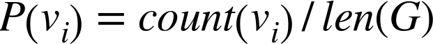
upper P left-parenthesis v Subscript i Baseline right-parenthesis equals c o u n t left-parenthesis v Subscript i Baseline right-parenthesis slash l e n left-parenthesis upper G right-parenthesis

What this means is that the frequency or probability P of a symbol v is the number of times that symbol occurs in set G (that is, count(v)), divided by the length of the set G.

Shifting from math to tables, let’s figure out the probability of each symbol inside of G. Because we have 10 symbols in G, len(G) is 10, and thus the probability for each symbols is a multiple of 0.1:

Symbol	Count	Probability
A	1	0.1
B	2	0.2
C	3	0.3
D	4	0.4
	Total must be:	1.0

With the probabilities for our unique symbols calculated, we can now go ahead and compute the Shannon entropy H of the set G. Gaze again upon this lovely formula; and fear not, as the gist is much simpler than you might think:

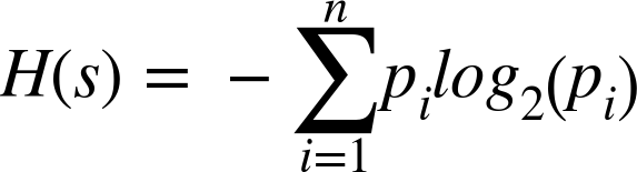
Firstly, for each symbol, multiply the probability of that symbol against log₂ of the probability of that symbol. Secondly, add it all up, and voilà, you’ve got your entropy for the set.

So, let’s apply this to G.

Symbol ∑	Probability p	log₂(p)	p * log₂(p)
1	0.1	-3.321	-0.3321
2	0.2	-2.321	-0.4642
3	0.3	-1.736	-0.5208
4	0.4	-1.321	-0.5284
		SUM	-1.8455

Summing that last column together gives a value of –1.8455 (give or take a few qubits). The Entropy equation applies a final sign inversion (that minus sign before the big ∑), giving us ~1.8455 bits per symbol to represent this dataset… Ta-da!

What This Entropy Stuff Is Good For

Because G = [A,B,B,C,C,C,D,D,D,D] has an entropy of H(G) = ~1.8455, we can roughly say that G can be encoded by using 2 bits per value (by rounding up to the next whole bit).

We assign the following 2-bit character encodings:

A -> 00

B -> 01

C -> 10

D -> 11

Our binary-encoded grouping G^e then looks like this:

e = [00,01,01,10,10,10,11,11,11,11]

With this encoding, we end up with a size of G^e (denoted as |G^e| in most texts) as 20 bits.

Now for the fun part: We can calculate the final size of G^e without having to actually do the encoding step. All we have to do is multiply the rounded-up⁵ entropy value H by the length of G (|G|):

H(G) * |G| = 2 * 10 = 20 bits = |G^e|

And according to Shannon entropy, that’s as small as you can make this data set.⁶

So, wrapping all this up, entropy generally represents the minimum number of bits per symbol, on average, that you need in order to encode your data set so as to produce the smallest version of it.

Understanding Probability

At its core, Shannon entropy is built upon the evaluation of the probability of symbols in the data stream, in an inverse sort of way.

Basically, the more frequently a symbol occurs, the less it contributes to the overall information content of the data set. Which…seems completely counter-intuitive.

We can find a real-world example of this in fishing. Suppose that you are sitting at the shoreline, reel and rod and fancy hat, in your lawn chair, watching the river and your bobber. Every few minutes, you take note of the state of the bobber, which remains unchanged. But every hour or so, a fish bites. That’s the thing you are interested in! So, very low information over a long time, with the occasional really important thing happening. If you represented the measurements you take with 0 for “no fish” and 1 for “fish!”, you could easily write your notes as 0000000010000000001000000000001.

Statistically (and sportingly!) speaking, the interesting parts are the events when the fish are biting. The rest is just redundancy.

But enough metaphor, let’s take a look at a few numerical examples. The next table shows some sets of probabilities (we don’t care about the actual symbols for now) and their associated entropies:

Probability set P(G)	Entropy H(G)	For a set of 1000 symbols…
[0.001, 0.002, 0.003, 0.994]	0.06	994 would be the same
[0.25, 0.25, 0.003, 0.497]	1.53	497 would be the same
[0.1, 0.1, 0.4, 0.4]	1.72	800 would be equally shared by two symbols
[0.1, 0.2, 0.3, 0.4]	1.84	One symbol would dominate but not by much
[0.25, 0.25, 0.25, 0.25]	2	Each symbol would occur 250 times

So, what’s going on here?

In the first row, the fourth symbol claims the overwhelming majority of the probability. This data set is dominantly composed of that one symbol, with a sprinkling of the others somewhere in it randomly. Because one symbol contributes to so much of the data stream’s content, it means there’s less overall information in the data set, hence the lower entropy value.

In the last row of the table, you can see that all four symbols are equally probable, and thus they contribute equally to the data stream’s content. The result is that there’s more information in the data set, and therefore we need more bits, per symbol, to represent it.

For example, playing whack-a-mole is interesting because all slots are equally probable, and you never know from which one the mole is going to pop up, which is what makes it a lot more interesting than fishing.

Breaking Entropy

The bleeding edge of data compression is all about messing with this entropy. In fact, the entire science of compression is about calling entropy a big fat liar on the Internet.

The truth is that, in practice,⁷ it’s entirely possible to compress data to a form smaller than defined by entropy. We do this by exploiting two properties of real data. Entropy, as defined by Shannon, cares only about probability of occurrence, regardless of symbol ordering. But ordering is one fundamental piece of information for real data sets, and so are relationships between symbols.

For example, these two sets, the ordered [1,2,3,4] and the unordered [4,1,2,3], have the same entropy, but you intuitively recognize that there is additional information in that ordering. Or using letters, [Q,U,A,R,K] and [K,R,U,Q,A] also have the same entropy. But not only does [Q,U,A,R,K] represent a word with meaning in the English language, there are rules about the occurrence of letters. For example, Q is usually followed by U.

Let’s look at some examples of how we can exploit these properties to break entropy. (Roll up your sleeves, we’re gonna compress some data!)

The key to breaking entropy is to exploit the structural organization of a data set to transform its data into a new representation that has a lower entropy than the source information.

Example 1: Delta Coding

Let’s take a set of increasing numbers, [0,1,2,3,4,5,6,7], and call it set A.

Now, shuffle that set to get set B = [1,0,2,4,3,5,7,6].

These two sets have a few unique characteristics with respect to information theory:

All the symbols are equally probable, and there are no duplicates.
Set A and set B have the same exact entropy of H = 3.

So, according to Dr. Shannon, we should assign 3 bits per symbol, requiring 24 bits total to encode each set. It turns out that it is possible to easily break entropy and encode set A in fewer bits. Here is how:

Set A is effectively just a linearly increasing run of numbers. So, instead of encoding each number, we could transform the stream and encode each number by its difference from the previous one. Set A encoded would then look like this:

[0,1,1,1,1,1,1,1]

And the entropy of this stream is only H(A) = 1. Not bad, eh?

This type of transform is known as Delta Coding, or the process of encoding a series of numbers as the difference from the previous number.⁸

So let’s talk about set B. Because it’s not linearly increasing, delta coding won’t really work on it, as we’d get [1,–1,2,2,–1,2,2,–1] with an entropy of H(B) = 2, which doesn’t look so bad at first. However, first we would need to encode the multiset⁹ B as [01,00,10,10,00,10,10,00] using a total of 16 bits. In addition, we’d also need to store for the decoder that the codeword “00” represents the symbol –1, which takes up additional space. So, not much of a win, if any. (In fact, for some sets, delta coding might even require more bits overall than just encoding the data directly.)

Example 2: Symbol Grouping

Suppose that you have a string S = “TOBEORNOTTOBEORTOBEORNOT”, which has the unique set of symbols [O,T,B,E,R,N] and entropy H(S) = 2.38.

Any human can look at this and realize that there are duplicate words here. So, what if instead of using individual letters as symbols, we used words? This gives us the unique set [TO,BE,OR,NOT] and an entropy of H(S) = 1.98.

So, if using words instead of symbols has given us a lower entropy value for the stream, how far can we take this? It looks like the term “TOBEORNOT” is used multiple times. Could we collapse that into one symbol?

Let’s just try that:

set(S)=[TOBEORNOT,TO,BE,OR] with an entropy H(S)=1.92¹⁰

Take that, entropy!¹¹

Example 3: Permutations

The interesting thing about set B [1,0,2,4,3,5,7,6] from Example 1 is that it’s a shuffled version, or permutation, of set A [0,1,2,3,4,5,6,7].

In mathematics, the notion of permutation relates to the act of rearranging, or permuting, all the members of a set into some sequence or order.

Effectively, a permutation is a shuffled version of an original set for which the order of elements matters, and no items are repeated. From a classical definition, permutations only exist as a shuffling of a run of numbers. For example [2,1,3,4] is a valid permutation of [1,2,3,4], whereas [5,2,7,9] is not.

Permutations are notoriously difficult to compress. (Some would say impossibly difficult, but we are not sure they really understand the meaning of that word). The reason for this is simple: according to entropy, a permutation is incompressible, because there’s no information in the ordering itself (because it’s not ordered anymore). Each value is equally probable, and thus takes the same number of bits to represent.

The size of the encoded set Q = [2,1,3,0] is len(Q) * log₂(max(Q)) = 8 bits,¹² which we can generalize to N * LOG2(N). Keep this number in mind. As you begin to explore more of compression, information theory, and entropy, this value will continue to kick you square in the face as a glaring reminder of how little you matter in the universe.

Compressing Permutations by Using Elimination Coding

So, remember how we said permutations weren’t compressible? We lied to you. It wasn’t a big lie, but it was a necessary lie to let you understand the gravity of the situation. We are sorry for that. In truth, permutations are slightly compressible, but not enough to be really interesting or of any practical use. Let us show you how.

Let’s begin with set C = [5, 7, 1, 4, 6, 3, 2, 0].

Encoding this by the number values in the set, with 3 bits, dictated by the maximum value 7, yields:

101 111 001 100 110 011 010 000

which is 24 bits long.

Now, let’s encode “by the index,” instead. It works like this. (You might want to follow along using old-fashioned paper and pencil.)

Round 1

Create an array with eight empty, indexed slots to hold the numbers.

Start with the first number in the set, which is 5.
Calculate its Free-Slot-Index: find the index of the slot with the value of our number. In our case, 5 is at index 5.
Determine how many bits you need to encode the Free-Slot-Index. This is done by calculating LOG2 of the number of slots. Because there are 8 slots, LOG2(8) = 3 bits. So, we encode the number 5 using 3 bits, which is 101.
Now, remove the slot with value 5 from the array.

The output stream contains: 101

The new working array is:

Round 2

Take the next number in the set C = [5, 7, 1, 4, 6, 3, 2, 0], which is 7.
Free-Slot-Index: find the index of the slot with the value of your number. This time, 7 is at index 6.
There are 7 free slots left, and LOG2(7) = 3. So, we output Free-Slot-Index 6 using 3 bits as 110.
Remove the slot with value 7 from the array.

Output stream: 101 110

New working array:

Round 3

Take the next number in C, which is 1.
Free-Slot-Index: find the index of the slot with the value of your number. In our case, it’s at index 1.
Calculate the LOG2 of the total number of free slots, where LOG2(6) = 3. Output the index 1 using 3 bits as 001.
Remove the slot with value 1.

Output stream: 101 110 001

New working array:

Round 4

The next number in the set is 4.
Its Free-Slot-Index is 3.
There remain 5 free slots, so LOG2(5) = 3 bits.
Output index 3 using the 3 bits as 011.
Remove the slot with value 4.

Output stream: 101 110 001 011

Round 5

Now things are finally starting to get interesting.

(We are halfway through our set [~~5, 7, 1, 4~~, 6, 3, 2, 0]).

Our next number is 6.
Its Free-Slot-Index is 3.
At this point, the number of free slots has dropped to 4, so LOG2(4) = 2, and we now only need 2 bits to encode an index.
Output 3 using 2 bits as 11.
Remove the slot with value 6.

Output stream: 101 110 001 011 11

Finishing up

The next number is 3.
It’s at Free-Slot-Index 2.
We encode with 2 bits as 10.
Remove the slot with value 3.

Output stream: 101 110 001 011 11 10

The next number 2, at Free-Slot-Index 1, can be encoded with 1 bit.
And we encode 0 with the last Free-Slot-Index, 0, using also 1 bit.

Final Output stream: 101 110 001 011 11 10 1 0

Length: 18 bits

And here is how this works out saving 6 bits. Look at the table to compare:

Instead of encoding the numbers, which would cost us 24 bits, by encoding the indexes, we only need 18 bits—a savings of about 25%. So, we’ve seen how this saves us bits, but...

Why does this save us bits?

Statistics says that for a permutation, there are N! (aka factorial(N)) possible combinations (for an array of length N, where each value is between 0–N and never repeated). So, when the first value is used, we know that it can’t be used again anywhere else. This means that for the second value, we have (N - 1)! options left. The third value has (N - 2)! options left (and so on). At some point, LOG((N - X)!) of the indexes will become less than LOG(N!) of the permutation by a full integer value. As such, we can identify which of the remaining options we have left, by using fewer bits.

This method works regardless of the size of the permutation. If you encode content this way, you’ll always be ensured to produce a final stream smaller than entropy. For example, if you have a permutation containing all of the numbers from 0 to 65,535, you can compress it to only 90% of the original space, regardless of how shuffled it is. In practice this doesn’t usually buy you enough space to make it worthwhile.

Decoding works in the opposite manner. You begin with a blank array of slots and read the next LOG2(#OpenSlots) bits from the stream, representing the number of blank spaces to count, to determine what the source number was.

We have 8 free slots, so we read the first 3 bits from the input stream, which are 101.
101 is the binary version of 5. At index 5 we have the number 5, so our first numbers is 5. Now we remove that slot from the free slot list.
We have 7 free slots, reading LOG2(7) = 3 bits, giving us 110, which is decimal index 6, so the next number is 7.
And now it’s your turn.

Information Theory Versus Data Compression

These simple experiments prove that there’s some wiggle room when it comes to information theory and entropy. Remember that entropy defines the minimum number of bits required per symbol, on average, to encode the data stream. This means that some symbols will use fewer bits and some will use more bits than indicated by entropy.

The algorithmic art of data compression is really about trying to break entropy. Or rather, to transform your data in such a way that the new version has a lower entropy value. That’s really the dance here: information theory sets the rules, and data compression brilliantly side-steps them with the gusto of a bullfighter.

And that’s really it. That’s what this entire book is about: how to apply data transformation to create lower entropy data streams (and then properly compress them). Understanding the dynamic between information theory and data compression will help you to put in perspective the give-and-take that these two have in the information world around us.

Kolmogorov Complexity

As we’ve already discussed, entropy is a horrible metric for evaluating compression.¹³

There exists another complexity measurement that might be more accurate, but it’s not really standardized in terms of usage.

Kolmogorov complexity is a measure of the computational resources needed to specify an object. It is named after Andrey Kolmogorov, who first published on the subject in 1963.

For example, consider the following two strings of 32 lowercase letters and digits:

abababababababababababababababab

4c1j5b2p0cv4w1x8rx2y39umgw5q85s7

We could write a simple program in Python to generate the first string:

< v = 'ab' * 16 >

Notice that the program to generate the string is smaller than the string itself. As an effective way of compression, you could just send the program to someone and have them regenerate the source string.

The second stream doesn’t follow a pattern, and so the program needed to generate it is much larger than the source stream; so, no compression here.

Here’s a handy primer:

Entropy: Number of yes/no questions needed to uniquely describe a piece of data.
Kolmogorov complexity: The size of the program needed to uniquely generate your data.

It can be shown that the Kolmogorov complexity of any string cannot be more than a few bytes larger than the length of the string itself (basically, a program that writes out each element of the string). Strings whose Kolmogorov complexity is small relative to the string’s size, like the ‘abab’ example above, are not considered to be complex.

Kolmogorov complexity really begins to shine when you start talking about using logic synthesis or program synthesis for compression, which in essence take the bit stream of your data set and reverse-generate a program that will uniquely generate it.

To be fair, this is all kinda hand-wavy. Entropy is far from the best solution, but it’s a “good enough” metric that most folks rely on it. Discovering a more accurate solution might involve a lot of random searches through data information and analysis space. The main point here is that, despite being around for almost 50 years, data compression science is still young. We don’t have all the answers, and really, that’s what you should be helping with.

¹ Shannon denoted entropy with the term H (capital Greek letter Eta), named after Boltzmann’s H-theorem.

² Note, the formula for H uses the mathematical definition of log₂(), which is different from the LOG2() we defined in Chapter 2. In this case, we don’t expect the output to be rounded up to the next highest integer, and the value is allowed to be negative.

³ You can find implementations of this algorithm in various languages over at Rosetta Code.

⁴ It doesn’t matter whether the values are sorted; that is, it has no effect on entropy, as we’ll see later in the chapter. We chose this ordering because it’s easy to see how many there are of each letter.

⁵ Remember that in practice we can’t represent fractional bits...yet.

⁶ Which is a complete and utter lie...but we’ll get to that in a minute.

⁷ Take that, “Theory”!

⁸ Don’t worry, we’ll talk about this in more depth in Chapter 8.

⁹ A multiset is a set for which multiple occurrences of the same element are allowed.

¹⁰ Of course, although in theory there is a difference between the two ways of grouping, for this tiny data set, in practice, we’d still need 2 bits either way. But remember that right now we are only concerned with beating Shannon.

¹¹ It’s worth pointing out that there’s a sweet spot with respect to symbol grouping, and an entire field of data transforms that help you find the optimal parsing; they are called “Dictionary Encoders,” and we will discuss them in Chapter 7.

¹² The maximum value of a set A of elements is denoted by max(A) and is equal to the last element of a sorted (i.e., ordered) version of A.

¹³ Well, to be fair, it’s really good at estimating the compression when only considering statistical compressors (see Chapter 4), but as soon as you begin combining them with contextual compressors, it kinda gets thrown out the window.

Previous Chapter

2. Do Not Skip This Chapter

Next Chapter

4. Variable-Length Codes