Table of Contents for
Understanding Compression
 Understanding Compression
Published by
O'Reilly Media, Inc., 2016
Understanding Compression
Published by
O'Reilly Media, Inc., 2016
- Cover
- nav
- Understanding Compression
- Understanding Compression
- section
- Foreword
- Preface
- 1. Let’s Not Be Boring
- 2. Do Not Skip This Chapter
- 3. Breaking Entropy
- 4. Variable-Length Codes
- 5. Statistical Encoding
- 6. Adaptive Statistical Encoding
- 7. Dictionary Transforms
- 8. Contextual Data Transforms
- 9. Data Modeling
- 10. Switching Gears
- 11. Evaluating Compression
- 12. Compressing Image Data Types
- 13. Serialized Data
- 14. Lossy Data Compression
- 15. Making the World a Little Smaller
- Glossary of Compression Words
- Index
- About the Authors
- Colophon
Chapter 8. Contextual Data Transforms
Before we begin with this chapter, let’s take a moment to recap.
Statistical encoders work by assigning a variable-length codeword to a symbol. Compression comes from smaller codewords being given to more frequently occurring symbols. The tokenization process of dictionary transforms works by identifying the longest, most probable symbols for a data set. Effectively, they find the best symbols for a set so that it can be encoded more efficiently. Technically speaking, we could just use the process to identify the best symbols and then plug that back into a statistical encoder to get some compression. However, the real power of the LZ method is that we don’t do that; instead, we represent matching information as a series of output pairs with lower entropy, which we then compress.
In addition to dictionary transforms, there’s an entire suite of other great transforms that work on the same principle: given some set of adjacent symbols, transform them in a way that makes them more compressible. We like to call these kinds of transforms “contextual,” because they all take into account preceding or adjacent symbols when considering ideal ways to encode the data.
The goal is always to transform the information in such a way that statistical encoders can come through and compress the results in a more efficient manner.
You could transform your data in lots of different ways, but there are three big ones that matter the most to modern data compression: run-length encoding, delta coding, and Burrows–Wheeler transform.
Let’s pick them apart.
Run-Length Encoding
Run-length encoding (RLE) is one of the most deceptively simple and powerful encoding techniques for various data types over the past 40+ years. RLE takes advantage of the adjacent clustering of symbols that occur in succession. It replaces a “run” of symbols with a tuple that contains the symbol and the number of times it is repeated. For example, as Figure 8-1 demonstrates, AAAABBBBBBBBCCCCCCCC is encoded as [A,4][B,8][C,8].1
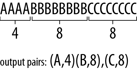
Figure 8-1. RLE identifies runs of identical symbols in a stream. It then transforms the stream into a set of pairs containing the symbol and the length of its run.
From a conceptual level, that’s really it. Nothing special after that. Encoding means finding a symbol and scanning ahead to see how long the run is.
Decoding works in the inverse. Given a pair containing the symbol and the length, simply append the proper number of symbols to the output stream.
Dealing with Short Runs
However, not all data is as uniform as our first example. Following the simplistic algorithm, AAAABCCCC would be encoded as [A,4][B,1][C,4]. Because the single B in the middle of the run was expanded from one symbol to a symbol-and-length pair, we have just created bloat in the data stream, as illustrated in Figure 8-2.
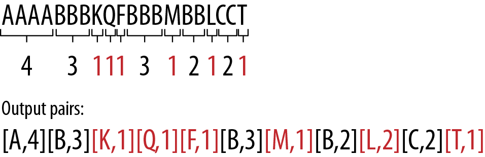
Figure 8-2. Small runs represent large problems for RLE as an algorithm. The overhead of storing short runs impacts the compression size significantly. Take this example, where the many nonduplicated symbols bloat the output.
Now if you’re lucky, across your entire stream the amount of overhead from these single symbols will easily be covered by the savings from long runs.
For all other situations, you need a way of identifying runs of characters that are worse off being encoded with RLE, and perhaps should be left alone in the stream, instead. For example, you could encode only runs with two or more symbols.
With that premise, AAAABCCCC would be encoded as [A,4] B [C,4]. Thus, if many characters are not repeated, you will rarely use an unnecessary counter. The problem with this method is that decoding is properly ambiguous. If we translate the transformed stream into binary, we could end up with 100000110010000101000011100,2 and no real way of distinguishing where the B run ends and the C run begins. Basically, the literal values being interwoven into the data stream is problematic.3
As such, we need a way to denote what runs have pairs and what runs don’t. A common solution to this is to add to the data set a second bit stream that denotes whether a given stream is long or repeated (Figure 8-3). Thus, the stream of 100000110010000101000011100 would be prepended by a bit stream of 101, denoting that the first symbol is a run, the second is not, and the third is. This helps save you the overhead of small-run streams by instead deferring a single bit-per-run.
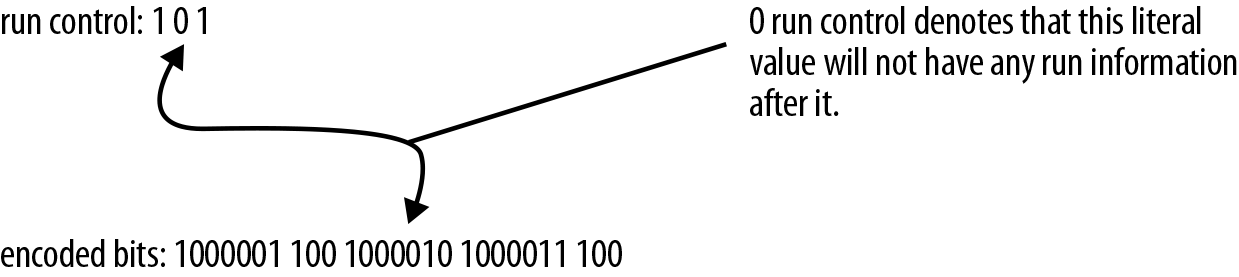
Figure 8-3. By combining a bit stream denoting which literals are runs, we can properly decode the stream. In this example, the second literal has a 0 for run control, so we don’t attempt to read the 3 bit code afterward, which would denote how long the run is.
Important
RLE works best on data sets with looooooooong runs of similar symbols. If your data set does not exhibit those characteristics, RLE won’t work for you, and you might want to keep reading and learn about MTF or delta coding, instead.
Compressing
Compressing an RLE’d stream is a bit of a trick. First, split your data set into two sets: a literal stream, and a run-length stream. (Remember the bit stream you prepended? It will tell you from which stream to read during decoding.) You can encode the literal stream by using an encoder of your choice.4 The run-length stream is really where the compression problems lie. So, using the very real-world method of trial and error, let’s find a suitable encoding for it.5
Given the lengths [4,3,1,1,1,3,1,2,1,2,1], we could encode them with binary 2 bits per value, giving us 22 bits total. However, this falls over if we get one run of long length, such as [256,3,1,1,1,3,1,2,1,2,1]. In this case, we’d need to encode all the values with the same number of bits as the largest value in the set. So in this case, we’d need to encode every value with 8 bits, making the set 88 bits total. Not ideal.
So, let’s move from that to static VLCs. In a naive model, we could assign a run-length integer with the number of bits from the representing VLC. So, if we had the lengths [4,3,1,1,1,3,1,2,1,2,1], we could end up with a unary encoding of [11110,1110,10,10,10,1110,10,110,10,110,10], or 31 bits. As you can see, this method fails directly. It assigns the smallest value to the smallest codeword (assuming that it appears most often in the data). RLE lengths are opposite, however, and we want to assign the largest values (representing the longest runs) with the smallest codewords.
Applying a statistical encoder (such as Huffman or arithmetic compression) might be better. We can get a sense of the impact of those values on our data set by calculating the set’s entropy, which is 1.69, giving us an encoded size of ~19 bits (about 13% savings). We could find a lower entropy by applying an adaptive version of a statistical encoder, which might take into account locality, if there is any.
RLE is considered a single-context model, in that any given symbol considers the previous symbol during encoding. If it’s the same, you continue on with the run, and if it’s different, you terminate the current run. Even though it’s not used often for modern compressors, more efficient RLE methods continue to be researched. For example, a new RLE compressor, TurboRLE, has been published recently, and it claims to be the fastest, most efficient RLE encoder of all time.
Delta Coding
We touched on delta coding a bit earlier, but it’s time to go into some deeper details. Numeric data must be some of the most annoying types of data to compress. This is because most of the time, there’s no statistical information to exploit. And you run into numerical data everywhere. Think GPS coordinates, inverted indexes from a search engine, and returning user IDs. Consider this lovely block of awesome as an example:
[51, 12, 8, 321, 0, 0, 12, 18, 9, 255, 0, 18, 64]
From an entropy perspective, there’s not a lot to work with here. Only a few values are duplicated, and the rest tend to have a high entropy value. In general, we’d need to store this data set in its full 8 bits per value. Thankfully, there’s a way to transform this data into a different set of numbers that might have better entropy.
Delta coding is the process of storing a data stream as the relative differences (deltas) between subsequent (i.e., adjacent) values. The idea is that, given a set of data, correlated or similar data tends to cluster around itself. If so, determining the difference between two adjacent values might be able to define one value as the difference from the other. Basically, you subtract the current value from the previous value and store that difference to your output stream.
Delta coding is one of the most important algorithms in modern computing. Given the fact that numeric data is so prevalent in our systems and its entropy is so high, delta coding offers a transform that’s not based on statistics; rather, it’s based on adjacency. It’s most helpful in time-series data (such as a sensor checking the differences in temperature once every 10 seconds), or in media, like audio and images, where locally there’s temporal correlation between data.
Take this set of numbers:
[1,3,6,8,10]
Perform the subtractions → and receive this delta-encoded set:
[1,3–1,6–3,8–6,10–8] → [1,2,3,2,2]
The source data roughly needed to be stored using 4 bits each (because log2(10) = 4). After delta coding, the resulting stream requires only 2 bits per symbol. The result? 10 bits instead of 20.
You can reconstruct the original stream by reversing the process. Adding the previous value to the current offset.
Start with the encoded set:
[1,2,3,2,2]
Perform the additions → and receive this original set:
[1,1+2,3+3,6+2,8+2] → [1,3,6,8,10]
In general, the goal of delta coding is to reduce the dynamic range of the data set. That is, reduce the number of bits needed to represent every value in the data. Which means that Delta coding is most effective when the differences between subsequent values are relatively small. If the differences between values become large, things break down.
Observe this set:
[1,2,10,256]
Perform delta coding → and receive this:
[1,2–1,10–2,256–10] → [1,1,8,246]
Applying delta coding here didn’t produce a less dynamic range, and we still need to encode the entire set with log2(maxValue).
But things could become even worse than that. Consider this sequence of woe:
[1,3,10,8,6]
Perform Delta coding → and cry:
[1,3–1,10–3,8–10,6–8] → [1,2,7,–2,–2]
In this set, we have subsequent values that are larger than their predecessors, and we end up with negative values in the transformed set. The largest positive value is 7, so we could store the positive values as LOG2(7) = 3 bits each. Sadly though, we now need to represent those negative values, meaning that we need to store an extra bit per symbol, requiring 4 bits.
These kinds of situations are extremely common and are exactly where delta coding falls over and becomes less effective. But there’s a whole slew of modifications you can apply to make this algorithm more robust, regardless of the data to which you’re applying it.
Let’s take a look at a few simple examples.
XOR Delta Coding
The issue with subtractive delta coding is that you can end up with negative values, which causes all sorts of problems. Negative values require you to store an extra lead bit, and they also increase the dynamic range of your data, like so:
[1,3,10,8,6] → [1,3–1,10–3,8–10,6–8] → [1,2,7,–2,–2]
We can improve this result by replacing subtractions with bitwise exclusive OR (XOR) operations.
Bitwise Exclusive OR (XOR) Operations
Bitwise operates on each bit independently. Exclusive OR (XOR) is a logical operation that outputs TRUE only when both inputs differ (one is TRUE, the other is FALSE).
Example:
    0101 (decimal 5)
XOR 0011 (decimal 3)
  = 0110 (decimal 6)
Note that you can use XORing with bit strings of 1 to flip bits.
     0101 (decimal 5)
XOR 1111 (decimal 15)
  = 1010 (decimal 10)
Also note that XORing any value with itself always yields 0.
In times long gone, when registers were flipped and cleared manually, this was indeed essential knowledge.
XORing bypasses the issue of negatives entirely, because XORing integers never generates negative values.
Starting with: [1,3,10,8,6]
XOR Delta encoded =
1 ⊕ 1 = 0
3 ⊕ 1 = 11 ⊕ 01 = 10 = 2
10 ⊕ 3 = 1010 ⊕ 0011 = 1001 = 9
8 ⊕ 10 = 1000 ⊕ 1010 = 0010 = 2
6 ⊕ 8 = 0110 ⊕ 1000 = 1110 = 14
Yields: [1,2,9,2,14]
So, this didn’t quite reduce the dynamic range, because we still need 4 bits per value, but it did keep all our values positive, regardless of the relative ordering of the data.
Frame of Reference Delta Coding
Consider the following sequence:
[107,108,110,115,120,125,132,132,131,135]
We could store these 10 numbers as 8-bit integers using 80 bits in total. But that seems a waste because all those numbers below 107 are just padding space. We’re including bits to potentially represent them, but our data set does not include any of those values.
The frame-of-reference approach addresses this problem by subtracting the smallest value from the rest of the numbers. In the example, the numbers range from 107 to 135. Thus, instead of coding the original sequence, we can subtract 107 from each value and delta encode this difference:
[0,1,3,8,13,18,25,25,24,28]
As a result, we can code each offset value using no more than 5 bits.
Of course, we still need to store the minimum value 107 using 8 bits, and we need at least 3 bits to record the fact that only 5 bits per value are used. Nevertheless, the total 8 + 3 + 9 * 5 = 45 is much less than the original 80 bits.
The “frame” part of “frame of reference” (also called “FOR”) has to do with the fact that to apply this transform to your data set properly, you need to subdivide it into smaller blocks (or frames) of numbers.
For instance, we could split our previous set of numbers into these two sets:
[107,108,110,115,120] [125,132,132,131,135]
We’d end up with the following:
[107,0,1,3,8,13] [125,0,7,7,6,10]
And framing our data has helped produce smaller dynamic ranges, and thus it requires fewer bits per value to represent.7
Sadly, outliers can still cause problems.
Patched Frame of Reference Delta Coding
Consider the following number set:8
[1,2,10,256]
Delta encoded =
[1,2–1,10–2,256–10] = [1, 1, 8, 246]
That outlier is basically breaking compression for the rest of the data.
To alleviate this problem, Zukowski et al.9 proposed a method of patching that they called PFOR.10
It works like this:
-
Choose a bit width b.
-
Walk through the data and encode numbers with b bits.
-
When you come to a number that requires more than b bits to encode, store this exception in a separate location.
The exceptions part of PFOR is where the magic comes in.
-
Consider our delta encoded example [1,1,8,246].
-
In a simplistic form, we could split the data into two sets, those values that require b bits and those that don’t. With b = 4 bits, we’d then get [1,1,8][246].
-
We can now encode the first set with 4 bits, and then the exception in 8 bits.
- To know where the exceptions get merged back into the source list, we also need a position value, giving us [1,1,8][246][3].
During the decoding phase, we take the exception values and insert them back into the source stream before undoing the delta decoding.
Of course, there are two main questions at this point:
-
How do we find the value b?
-
What do we do with the exceptions?
Finding b
The goal is to determine the proper bit width b that encodes the most numbers in our set and lets us identify outliers.
You can generally do this incrementally. Begin with 1 bit, test how many values in your set are less than 21. If 90% of your data is less than this value, set b = 1. Otherwise, increment b to 2, test for < 22. If necessary, repeat with b = 3 and 23, and continue until you find the b that works for 90% of your data set.
What do we do with exceptions?
One of the interesting problems with PFOR is that, along with your modified delta information, you now end up with a second data set that represents exception data. This second set can have a large dynamic range, and can be difficult to directly compress. According to the original papers, rather than just throwing the entire exception list into a new list, raw, PFOR can instead leave the lowest “b” bits in the source stream, and store the difference in the exception list.
For example, in the following list, the upper three most-significant bits are zeros, except in one number.
1010010
0001010
0001100
0001011
Now, rather than storing an exception set of 101,000,000,000, we can just note that the first location is the only exception we need to care about. The result, is that we now get three new sets.
The first set is the lowest 4 bits of our data:
[0010,1010,1100,1011]
Followed by an index to which values have an exception:
[0]
Followed by the actual exception bits, for those locations:
[101]
The result is that the exception array has a much lower dynamic range and can then be compressed a little better, potentially.
Compressing Delta-Encoded Data
Note that at this point, we haven’t actually compressed anything; we’ve merely transformed the data in such a way that things can potentially be more compressible.11
Delta coding produces a more compressible data set when it can do the following:
-
Reduce the maximum value in the stream, reducing the dynamic range.
-
Produce lots of duplicate values, which allows for more effective statistical compression.
The second is most likely more important because it fits in better with common statistical compression systems. However, if the results of delta coding don’t produce statistically variant data, you end up needing to take advantage of the first, which basically moves toward trying to reduce the overall LOG2 for the entire data set.
In general, taking the produced data and then throwing it at any statistical encoder should produce good compression.
Move-to-Front Coding
Contextual data transforms operate on the basic philosophy that the linearity of the data (that is, its order) contains some information that helps us encode future symbols. Move-to-front (MTF) is such an encoding. But rather than considering immediate adjacency, like RLE and dictionary encoders do, MTF is more concerned with the general occurrence of a symbol over short windows of data.
The MTF step reflects the expectation that after a symbol has been read from the input stream, it will be read many more times, and will, at least for a while, be a common symbol. The MTF method is locally adaptive because it adapts itself to the frequencies of symbols in local areas of the input stream. The method produces good results if the input stream satisfies this expectation; that is, if it contains concentrations of identical symbols (if the local frequency of symbols changes significantly from area to area in the input stream).
Figure 8-4 shows that the entire process works by keeping a second array of data, which contains the unique values that exist in the data set. Let’s call this the SortedArray. As a value is read from the input stream, we find its location in the SortedArray and output that index to the output stream. Then, we update the SortedArray by moving that value to the front of the array, giving it an index of 0.
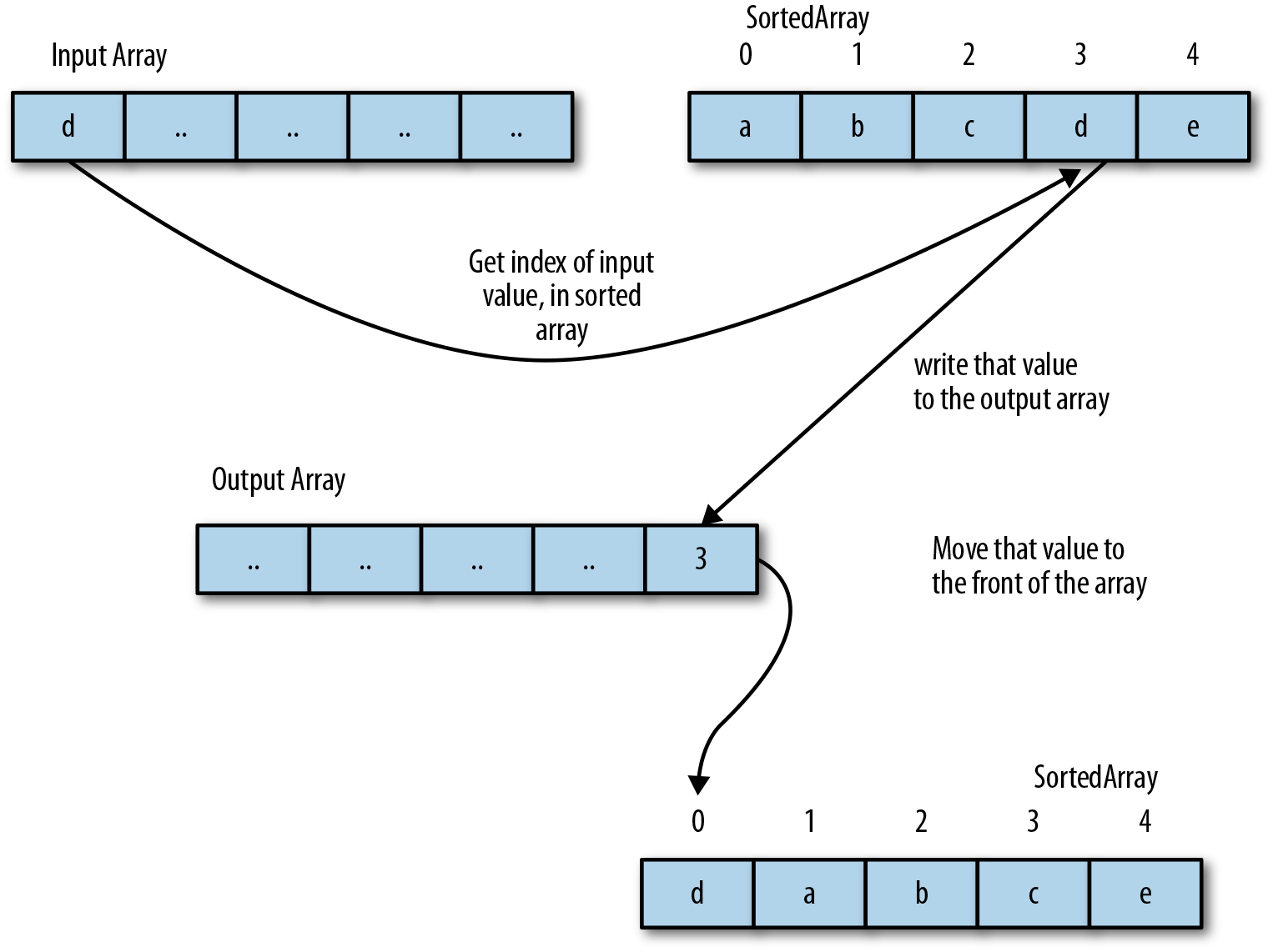
Figure 8-4. A general diagram detailing how MTF works. As a value is met in the input stream multiple times, it will move toward the front of the SortedArray, resulting in lower values being emitted to the output stream.
Here’s a simple example. Assume for simplicity’s sake that the symbols in the data are lowercase ASCII characters, that our input stream is “banana”, and that the symbols in our initial SortedArray are in alphabetical order:
-
Read the letter “b.”
-
“b” is at index 112 in SortedArray, so we output 1 to the output stream.
-
Move “b” to the front of SortedArray.
-
Read the letter “a,” which is now at index 1, output 1, and move “a” back to the front.
-
Continue with the remaining letters, moving through the table.
| Input symbol | Output stream | Re-SortedArray |
|---|---|---|
|
|
||
|
b |
1 |
|
|
a |
1,1 |
|
|
n |
1,1,14 |
|
|
a |
1,1,14,1 |
|
|
n |
1,1,14,1,1 |
|
|
a |
1,1,14,1,1,1 |
|
The final output stream is 1,1,14,1,1,1, which has an entropy of 0.65,13 as opposed to the source stream entropy of 1.46.
The decoder can recover this stream by reversing the process. Given [1,1,14,1,1,1], it starts with a SortedArray of [a,b,...z]. For each symbol the decoder reads from the input stream, it outputs the value at that index in the SortedArray, and then moves that symbol to the front of the SortedArray.
Avoiding Rogue Symbols
One of the issues with MTF is that a few rogue symbols can interrupt a nice stream of symbols that exist at the front. This is one of the more detrimental issues because it can seriously mess up your encoding, and in truth, it’s quite common in real-life data.
One solution to this is to not let symbols go to the very front of the list as soon as they are matched; instead, you need to employ some heuristic that slowly moves them to the front. The following example demonstrates how heuristics work quite well in practice.
Move-ahead-k
In this variant, the element of SortedArray that matches the current symbol is moved k positions toward the front, instead of all the way.
You need to figure out the optimal value for k; however, there are two easy choices:
-
Setting k = n (the number of symbols) is identical to the original MTF.
-
Setting k = 1 allows symbols to move to the front only one step at a time.
Setting k = 1 tends to reduce performance for inputs that have local concentrations of symbols, but works better for other inputs. Implementing the algorithm with k = 1 is especially simple because updating SortedArray only requires swapping an element with the one preceding it. This variant deals somewhat better with rogue symbols because they must slowly work their way to the front of the stream, rather than going there immediately.
Wait-c-and-move
In this variant, an element of SortedArray is moved to the front only after it has been matched c times to symbols from the input stream (not necessarily consecutive times). Each element of SortedArray has a counter associated with it to count the number of matches. This makes it possible for you to consider a threshold of occurrence before a symbol can approach the front of the stream. When used on text, this will tend to produce a SortedArray that mirrors the commonness of the letters in the language you’re encoding.
Compressing MTF
MTF creates a stream of symbols that is expected to have a lower entropy than the source stream. This makes its output a prime candidate to pass off to a statistical compressor for further compression. Because MTF should produce a stream with more 0s and 1s, a simple statistical encoder would work fine.
MTF is unique in that it reassigns a shorter value to symbols as they recur within a short time. RLE, on the other hand, assigns the shortest codes to symbols that occur in clusters. In practice, MTF is one of the simplest forms of dynamic statistical transforms.
Burrows–Wheeler Transform
Every family has a black sheep. Burrows–Wheeler transform (BWT) is one of them. You see, all of the other compression algorithms can generally be categorized as statistical compressors (i.e., VLCs) or dictionary compressors (such as LZ78), which in different ways exploit the statistical redundancies present in a given data stream.
BWT does not work this way. Instead, it works by shuffling the data stream to cluster symbols together. This does not provide compression in and of itself, but it lets you hand off the transformed stream to other compression systems.
Ordering Is Important!
One of the issues with entropy as a unit of measure is that it fails to take into account the order of the symbols. Regardless of how we shuffle [1234567890], it always has an entropy of 4.
But we know that order does, in fact, matter greatly. For example, the LZ family of dictionary compressors takes ordering very seriously, as do the other contextual transforms we’ve shown in this section.
So if order matters, it stands to reason that if we transform the order of a data stream, we can make it more compressible.
The simplest reordering here is to simply sort our data. For example, converting [9,2,1,3,4,8,0,6,7,5] to [0,1,2,3,4,5,6,7,8,9] makes it possible for us to delta encode it as [0,1,1,1,1,1,1,1,1,1], which has a lower entropy than the source.
Sadly though, pure sorts are one-directional. That is, after you sort the data, you can’t get it back into its unsorted form without a ton of extra information to specify where it goes.
So we can’t purely sort our data, but we can get close.
BWT shuffles the data stream and attempts to cluster groups of the same symbol near one another, which is what we call a lexicographical permutation. Or rather, with BWT you can find a permutation of the original data set that might be more compressible based on its ordering.
And here’s the best part: we can encode to and decode from BWT without having to add significant additional data to our stream. Let’s take a look.
How BWT Works
The “transform” part of Burrows–Wheeler transform begins by creating a table with all the shifted permutations of the input stream.
For example, we have the word BANANA, again, and write that in the first row of our table. Then, on each following line we perform a rotational shift to the right by one character of that word. That is, shift all the letters over to the right, and prepend the rightmost character at the front. We continue with this shifting, until we’ve touched each letter in our input string, as shown here:
|
BANANA |
|
ABANAN |
|
NABANA |
|
ANABAN |
|
NANABA |
|
ANANAB |
|
BANANA |
Next, the BWT algorithm sorts this table lexicographically by the bolded letters as shown in the example that follows. Feels good to have things back in order, doesn’t it?
|
ABANAN |
|
ANABAN |
|
ANANAB |
|
BANANA |
|
NABANA |
|
NANABA |
Now, we want to draw your attention to the last column of characters in the preceding example (highlighted in italics). From top to bottom, they form the string NNBAAA, which interestingly enough, is a permutation of BANANA, and has a much better clustering of letters.
And this is exactly the permutation that we’re looking for. You see, by generating our rotated permutations and then lexicographically sorting them, the final column generally produces a permutation with a better symbol clustering than the original source string.
As such, NNBAAA is what BWT should return as its output.
But before you run off, there’s one other piece of data we need to grab as well. Notice in the sorted table that follows, that the input string sits at index 3.
|
0 |
ABANAN |
|
1 |
ANABAN |
|
2 |
ANANAB |
|
3 |
BANANA |
|
4 |
NABANA |
|
5 |
NANABA |
We’ll need that row index during the decode phase of the BWT transform because it will allow us to bridge from our more-compressible permutation back to the source string.
Inverse BWT
The remarkable thing about the BWT is not that it generates a more compressible output—an ordinary sort could do that—but that this particular transform is reversible, with minimal data overhead.
Let’s illustrate this to confirm that it’s true. So, we want to decode a BWT, and we’re given the string NNBAAA and the row-index 3.
The first thing we need to do is regenerate the permutation table. To do this, we iterate on a combination of sorting and string appending.
We begin by writing our output string, which represents the last column, into a table.
| Output string/last column |
|---|
|
[N] [N] [B] [A] [A] [A] |
Oddly enough, if we sort this column, it is the same as the first column in our original, sorted table.14
| Output string | Sorted |
|---|---|
|
[N] [N] [B] [A] [A] [A] |
[A] [A] [A] [B] [N] [N] |
So, let’s merge these two columns to get a pair of letters for each row:
| [NA] |
| [NA] |
| [BA] |
| [AB] |
| [AN] |
| [AN] |
Let’s sort that:
| [AB] |
| [AN] |
| [AN] |
| [BA] |
| [NA] |
| [NA] |
Next, we prepend the original output string (NNBAAA) to it again:
|
[NAB] |
|
[NAN] |
|
[BAN] |
|
[ABA] |
|
[ANA] |
|
[ANA] |
Then, we sort again and continue prepending and sorting columns, until the width of the matrix equals the length of the output string.
|
3 |
4 |
5 |
6 |
7 |
8 |
9 |
10 |
|---|---|---|---|---|---|---|---|
|
[ABA] [ANA] [ANA] [BAN] [NAB] [NAN] |
[NABA] [NANA] [BANA] [ABAN] [ANAB] [ANAN] |
[ABAN] [ANAB] [ANAN] [BANA] [NABA] [NANA] |
[ABAN] [ANAB] [ANAN] [BANA] [NABA] [NANA] |
[NABAN] [NANAB] [BANAN] [ABANA] [ANABA] [ANANA] |
[ABANA] [ANABA] [ANANA] [BANAN] [NABAN] [NANAB] |
[NABANA] [NANABA] [BANANA] [ABANAN] [ANABAN] [ANANAB] |
[ABANAN] [ANABAN] [ANANAB] [BANANA] [NABANA] [NANABA] |
You should immediately notice two amazing properties of this final matrix:
-
This final matrix is identical to the post-sorted permutation matrix that we generated in the encoder. This means that if we’re given the final column of our sorted matrix, NNBAAA, we can recover the entire post-sorted matrix that was used to generate it.
-
Remember that row index 3 that we output during the encoding phase? Because this matrix is identical to the post-sorted one from the encoder, we simply need to look at the row at that index the fourth row to recover our source input string BANANA.
Practical Implementations
Be warned!
Even with all this wonderfulness, sadly you can’t just execute BWT on your entire 50 GB file. The way this permutation transform works, you’d have to store that same 50 GB, shifted left one symbol, for each row. That’s an awful lot of extra gigabytes.
As such, BWT is what we call a block sorting transform. It breaks the file into 1 MB chunks and applies the algorithm to each of them independently. The result is an algorithm that can practically fit in the memory of most modern devices and is somewhat performant.
Compressing BWT
So, it’s apparent that BWT doesn’t actually compress the data, it just transforms it. To practically use BWT, you need to apply another transform that is going to yield a stream with lower entropy, and then compress that.
The most common algorithm is to take the output of BWT and pass it to MTF, which is then followed by a statistical encoder. That’s basically the inner workings of BZIP2, folks.
Why not LZ?
Why can’t we use, say, LZ for this data? Well, let’s take a look at a simple example. Remember that LZ works best when it can find duplicate symbol groupings for long chains.
TOBEORNOTTOBEORTOBEORNOT works well because TOBEORNOT is the longest duplicated symbol found. However, this doesn’t work too well for runs of similar symbols.
Consider that if we ended up with “OBTTTTTTOOEER”:
-
The LZ algorithm would look at the first T and encode it as a literal.
-
The second T would be encoded as a previous reference of 1, and length of one.
-
The third T will look ahead 1 and encode the TT pair as a previous ref of 2, and length of two. The result, is that our 6 “T” values would generate: Literal T,<–1,1>,<–2,2>,<–2,2> as tokens.
Later on, if we hit a stride of “T” values again, we can hope for a long stride match; but sadly, because BWT groups these symbols so far apart, the distance reference would be quite large, which will affect how we encoded that stream.
1 According to “every CS class ever made” and Wikipedia, RLE encoding is typically introduced not as a pair-wise transform, but instead would inline the length with symbol values, giving A4B1C4. Truth is, though, that no one actually uses RLE in this form due to the interweaving of literal symbols and numeric values; so it’s a complete waste of time to introduce it that way. In fact, we are somewhat sad to have distracted you enough with this footnote by it—sorry about that.
2 If your eyes just glazed over, that’s 7 bits of ASCII per literal, so 1000001|100|1000010|1000011|100.
3 This is a problem we’ve already had to tackle in this book for adaptive statistical encodings and dictionary transforms: interleaving the literal values in the numeric stream is just asking for trouble.
4 LZ is fun to apply, because now you get to look at how often runs of symbols can be duplicated.
5 Even compressors that have multiple algorithms in their arsenal might choose in this manner.
6 S. W. Golomb, “Run-length encodings”, IEEE Trans. Information Theory, vol. IT-12, pp. 399–401, July 1966.
7 The elephant in the room is, of course, how to determine the optimal frame. So far, most implementations have used 32-bit to 128-bit windows, because…well, that fits into a single integer.
8 We know, you’ve already considered it once in this chapter. So this time, consider it harder.
9 M. Zukowski, S. Heman, N. Nes, and P. Boncz, “Super-Scalar RAM-CPU Cache Compression,” Proceedings of the 22nd International Conference on Data Engineering, ICDE ’06, IEEE Computer Society: Washington, DC, USA, 2006; 59–71, doi:10.1109/ICDE.2006.150
10 It’s worth noting that PFOR could, technically be applied to a data set independent of Delta coding, which is why you see this algorithm sometimes written as PFD, PFor or PForDelta when used in conjunction with delta coding. Which is how we like to use it, and why it’s in this section—it’s good to be the authors.
11 In fact, if you reread the previous sections, you’ll note that we were very clear to call this technique “delta coding” instead of “delta compression,” because technically speaking, the latter is incorrect; there’s no compression going on.
12 For nonprogrammers: array indices start at 0, so the second position in SortedArray is 1.
13 This really should give Shannon a headache. This is the lowest entropy we have seen in this book, so far.
14 This is not just because BANANA is an oddly shaped word. It’s an observed property of BWT that we exploit, and even the BWT authors don’t know why it exists.