Table of Contents for
Understanding Compression
 Understanding Compression
Published by
O'Reilly Media, Inc., 2016
Understanding Compression
Published by
O'Reilly Media, Inc., 2016
- Cover
- nav
- Understanding Compression
- Understanding Compression
- section
- Foreword
- Preface
- 1. Let’s Not Be Boring
- 2. Do Not Skip This Chapter
- 3. Breaking Entropy
- 4. Variable-Length Codes
- 5. Statistical Encoding
- 6. Adaptive Statistical Encoding
- 7. Dictionary Transforms
- 8. Contextual Data Transforms
- 9. Data Modeling
- 10. Switching Gears
- 11. Evaluating Compression
- 12. Compressing Image Data Types
- 13. Serialized Data
- 14. Lossy Data Compression
- 15. Making the World a Little Smaller
- Glossary of Compression Words
- Index
- About the Authors
- Colophon
Chapter 7. Dictionary Transforms
Even though information theory was created in the 1940s, Huffman encoding in the 1950s, and the Internet in the 1970s, it wasn’t until the 1980s that data compression truly became of practical interest.
As the Internet took off, people began to share images and other data formats that are considerably larger than text. This was during a time when bandwidth and storage were either limited, expensive, or both, and data compression became the key to alleviating these bottlenecks.
Note
With mobile devices on the march to world dominance, we are actually experiencing these same bottlenecks all over again today.
Although variable-length coding (VLC) was churning away at content, the fact that it was locked to entropy produced a limiting gate on the future of compression. So, while the majority of researchers were trying to find more efficient variable-length encodings,1 a few researchers found new ways for preprocessing a stream to make the statistical compression more impactful.
The result was what’s called “dictionary transforms,” which completely changed the mentality and value of data compression with respect to the masses. Suddenly, compression became a useful algorithm for all sorts of data types. So useful, in fact, that all of today’s dominant compression algorithms (think gzip or 7-Zip) use a dictionary transform as their core transformation step. So, let’s see what it’s all about.
A Basic Dictionary Transform
Statistical compression mostly focuses on a single symbol’s probability in a stream, independent of adjacent symbols that might exist around it. This is great for compressing Pi to the Nth digit, but does not take into account an essential property of real data: context, groupings, or simply put, phrases.
Note
There are “phrases” in other contexts, too: the rules of music, color composition in images, or the beating of your heart. Basically, any place where there’s a grouping of similar content that’s available to be repeated later.
For example, rather than encoding each letter of the phrase “TO BE OR NOT TO BE” as a unique symbol, we could, instead, use actual English words as our tokens. The result would create a symbol-to-codeword table that could look something like this (ignoring spaces):2
| Symbol | Frequency | Codeword |
|---|---|---|
|
TO |
0.33 |
00 |
|
BE |
0.33 |
01 |
|
OR |
0.16 |
10 |
|
NOT |
0.16 |
11 |
Which would give us 000110110011 for the encoded string. An original, per-letter encoding would have produced 104 bits, where the word-specific version was compressed to 12 bits.
When we stop considering single symbols, and instead begin considering groups of adjacent symbols,3 we move out of statistical compression and into the world of dictionary transforms.
Dictionary transforms work much like you’d expect. Given a source stream, first construct some dictionary of words (rather than symbols), and then apply statistical compression based on the words in the dictionary.
Dictionary transforms are not meant to be a replacement for statistical encoding, but rather a transform that you first apply to your stream, so that it can be encoded more effectively by a statistical encoder, as shown in Figure 7-1.
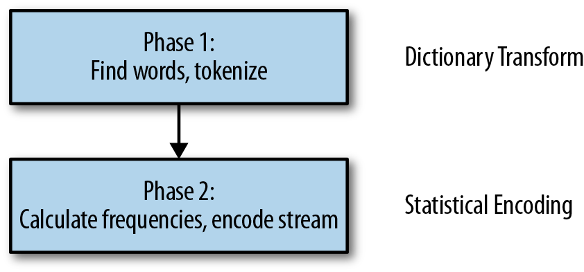
Figure 7-1. Applying a dictionary transform first can produce a data stream that can then be compressed more effectively by statistical encoding.
As such, dictionary transforms represent a preprocessing stage that’s applied to a data stream to produce a data set that is smaller and more compressible than the source stream.
A dictionary transform is most effective when it can identify long often-repeated substrings of the data, and assign them the smallest codewords.
Finding the Right “Words”
One big question is, “What represents the best words?” Well, the best words are those that in combination result in the smallest entropy. The bigger question is: How do we determine what those words are?4
Our previous example might have been a bit too easy, given that we could split on the spaces in the string and use our very eyes to identify the duplicates.
What about this next string? Looks a bit tougher, maybe?
TOBEORNOTTOBEORTOBEORNOT
Given that there’s no simple way to separate words out in this string (without teaching your computer the English language), how do you go about finding them?
You do it by using a process known as tokenization, which is parsing a set of data to find the ideal “words.” Tokenization is so complex that it has its very own branch of research (and associated patents) in the information theory field. For this book, we are going to stick with the basics.
As a baseline, let’s first take a look at what our example stream would look like, if we tokenized with single-symbol values—that is, by the letters:
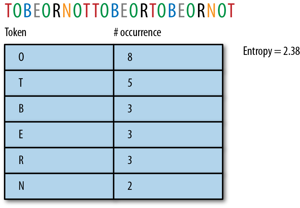
Tokenizing by the letters, we end up with an entropy of about 2.38, given that the letters “O” and “T” are duplicated often.
So that’s good to know, but let’s go the other way. Instead of the smallest symbols, let’s tokenize around the longest substring that repeats in the string:
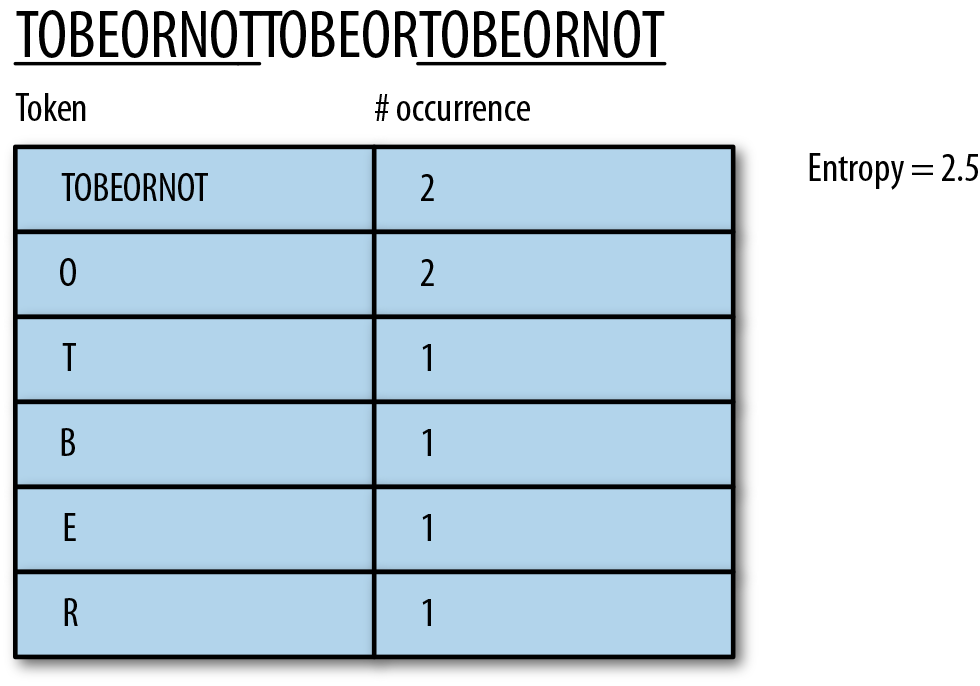
The longest string is “TOBEORNOT”, and it is matched twice in the input string. If we assign it a single codeword, the entropy of such a tokenization is about 2.5, which is larger than just using our single-symbol stream, so not a win for our data.
The reason for the increase in entropy is that now there is no clear skewing of the data toward a single dominant symbol. [O,T,B,E,R,TOBEORNOT] are roughly equally probable in this scenario, and thus, are assigned (roughly) the same number of bits.
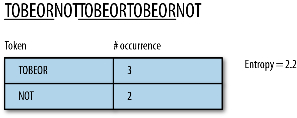
We could instead parse around the most frequent substrings, which would yield the tokens TOBEOR and NOT. This results in an entropy that’s better at 2.2, but not particularly impressive:
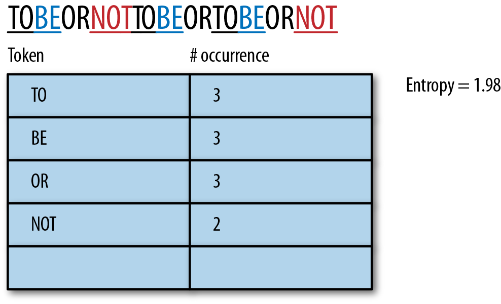
So, let’s try a different approach and tokenize by finding the shortest words with a length greater than 1: TO, BE, OR, NOT and an entropy of 1.98, which is the best we’ve found for this example:
Ah, so we’re back to parsing the string based on English words. Although this setup produces the lowest entropy, it’s difficult to see how you would properly parse a string to create these optimal sizes.
A brute-force method would read in a group of symbols (“TO”) and search the rest of the string to determine its frequency. If the frequency was a good match for the existing symbol table, the algorithm could continue on to the next symbol group and repeat the process. Otherwise, it would try a different group of symbols (such as “TOB”). Sadly though, this would not only require a lot of memory, but take a very long time for any real-life data stream. As such, it’s not really suited to any type of real-time processing.
The truth is that to find the ideal tokenization for a stream, we need some way to process symbols we haven’t come across before and those that we have, alongside the ability to combine them into the longest symbol sets possible, in some sort of performant manner.
The Lempel-Ziv Algorithm
In 1977, researchers Abraham Lempel and Jacob Ziv invented a few solutions to this “ideal tokenization” problem. The algorithms were named LZ77 and LZ78 and are so good at finding optimal tokenization, that in 30+ years, there hasn’t been another algorithm to replace them.
How LZ Works
LZ creates a tokenization by trying to match a current word with a previous occurrence of that same word. Rather than reading in a few symbols and then searching ahead to see if there might be duplicates, LZ works by instead looking behind to see if this word has been seen before. This has two main ramifications to the encoding process (see Figure 7-2):
-
Earlier in the stream, you’ll have seen fewer words, so incoming words will more likely be new. Later in the stream, you’ll have a larger buffer to pull from, and matches are more likely.
-
Looking backward lets you find the “longest matching word.”
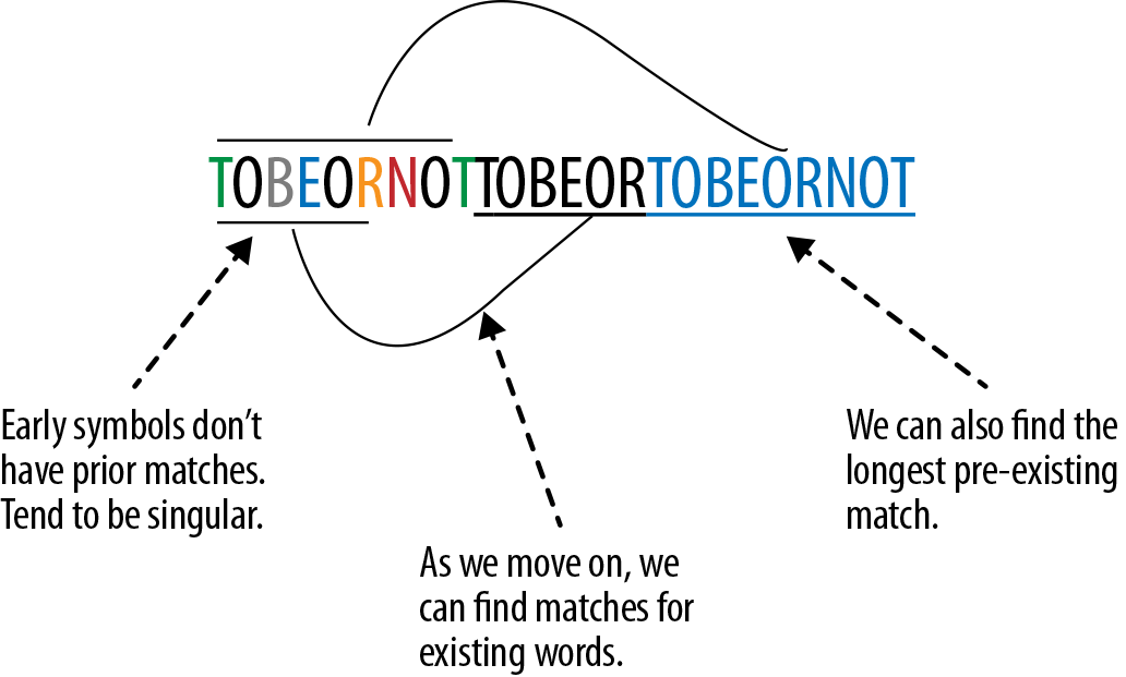
Figure 7-2. The LZ algorithm looks backward to find the longest previously encountered matching word.
The search buffer
The backbone of the LZ algorithm works by splitting the stream into two segments.
-
The left side of the stream is dubbed the “search buffer”; it contains the symbols that we’ve already encountered and processed.
-
The right side of the stream is dubbed the “look ahead buffer”; it contains the symbols we’re looking to encode.
As such, the current “reading” position in the stream is at the point between the two buffers, as demonstrated in Figure 7-3.
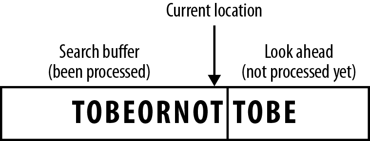
Figure 7-3. The search buffer and look ahead buffer are separated by the current reading location in the stream.
Finding matches
Finding matches is a bit of an organic interplay between the look ahead and search buffers.
Figures 7-4 through 7-9 show how this works.
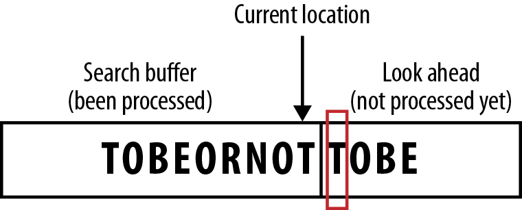
Figure 7-4. From the current location, read one symbol, which is T.
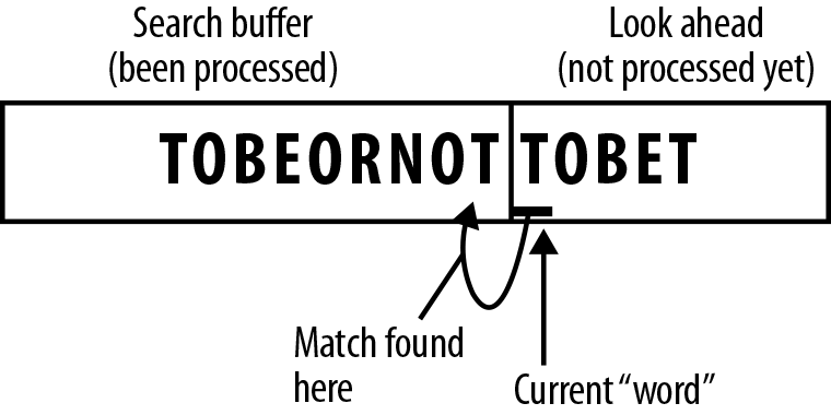
Figure 7-5. Search backward in the search buffer. The first symbol we see is a matching T.
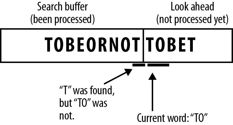
Figure 7-6. Because we are looking for the longest possible match, we now read a second symbol from the look ahead, which is O.
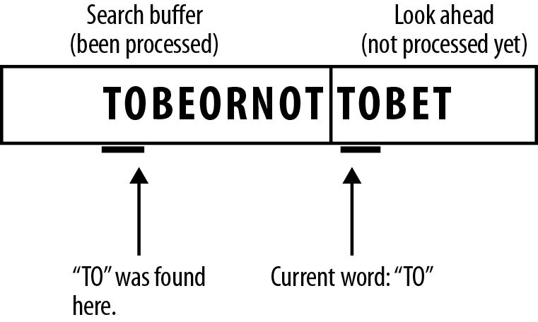
Figure 7-7. There is no O after our matched T in the search buffer, so we go further backward, until eventually we find TO.
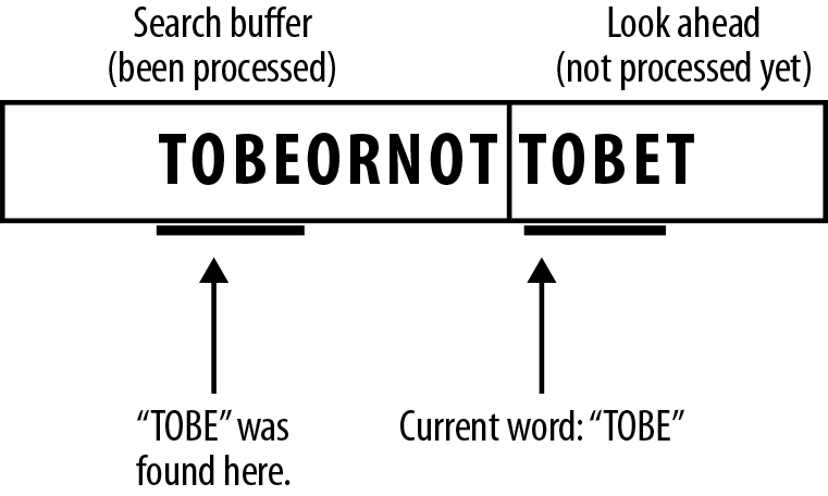
Figure 7-8. We now read the next symbol B, and we still have a match…and the next symbol E, and we are still matching, but looking at the next symbol T, it no longer matches, so we have found the longest match for this sequence of symbols.

Figure 7-9. We encode this match (as described in the next section) and shift the “current position” of the stream to the end of the longest matched word in our look ahead buffer, and … GOTO 1.
The “sliding window”
Now, in practical implementations, where the stream may be millions of tokens long, we can’t look back at the entirety of our already processed stream. Keeping an indefinite search buffer would run into memory and performance problems. As such, the search buffer typically only includes the last 32 KB of processed symbols. So, as we move the current location, we also move a sliding window search buffer along our stream, as illustrated in Figure 7-10.
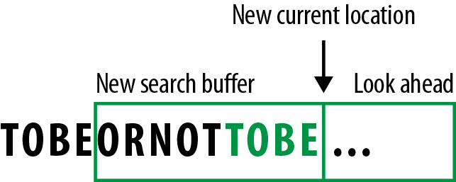
Figure 7-10. After we find a match and encode it, we shift the “current position” to the end of the longest matched word in the look ahead buffer, and the sliding window search buffer moves up to the new current location.
Having a sliding window puts an upper limit on the performance required to find a match. It also makes assumptions about locality, namely that there is a higher chance of correlated data existing at locally similar points in the given data set.
Note
In general, the sliding window search buffer is some tens-of-thousands of bytes long, whereas the look ahead buffer is only tens of bytes long.
Marking a match with a token
When a match is finally settled on, the encoder will generate a fixed-length token to an output stream. A token is made up of primarily two parts: offset and length.5
- Offset value
-
This represents the position of the start of the matched word in the current search buffer, working backward from the current position. In our example, the matched string was found nine symbols back from the current position mark.
- Length value
-
This represents the length of the matched word. In our example, the match was four symbols long.
Because for our example we found a match 9 symbols back in the search buffer, with a match-length of 4, the pair [9,4] is emitted to the output as our token, as shown in Figure 7-11.
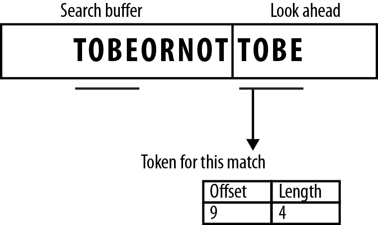
Figure 7-11. Tokens in the look-ahead buffer that match tokens in the search buffer are encoded with their offset from the matching token and their length.
The decoder will un-transform these values in very simple ways:
-
Read the next token
-
From the current position, count offset symbols backward in the search buffer
-
Grab the length number of symbols and append them to the data stream
When no match is found
There are situations for which no match is found in the search buffer for the symbol in the look ahead buffer. In this case, we need to emit some information that lists this new token, so that the decoder can recover it properly.
To do this, we emit a modified token that signifies that our output is a literal value, which the decoder can read and recover to the stream. How this token is constructed is entirely up to the flavor of LZ implementation. As a most basic approach, the algorithm would output a token that has 0 for its offset and 0 for its length [0,0], followed by the literal symbol, as shown in Figure 7-12.
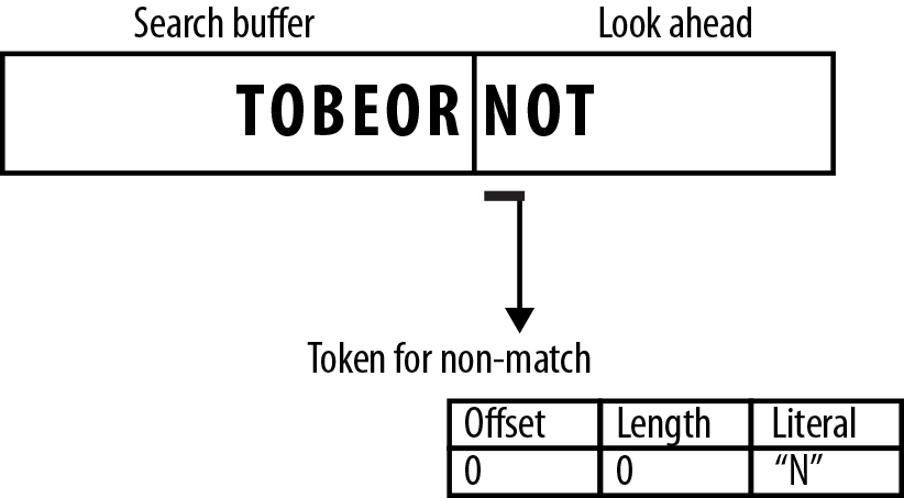
Figure 7-12. Tokens for nonmatched symbols are unique and typically include the literal symbol for the decoder to read.
Encoding
Given our input stream “TOBEORNOTTOBE”, let’s walk through an example encoding (see also the table that follows).
-
The first four symbols have no match in the search buffer, and are easily output to literal tokens.
-
When we get to the second letter “O” in the look ahead, we find a single matching symbol in the search buffer, giving us a token of (3,1).
-
This process continues on for a while, finding either nonmatches or single-value matches.
-
Where things get interesting, is when we get to the end of the string, and see TOBE matched, back at the beginning of the search buffer, at location 9 and with a length of 4.
| Search buffer | Look ahead buffer | Output |
|---|---|---|
|
TOBEORNOTTOBE |
0,0,T |
|
|
T |
OBEORNOTTOBE |
0,0,O |
|
TO |
BEORNOTTOBE |
0,0,B |
|
TOB |
EORNOTTOBE |
0,0,E |
|
TOBE |
ORNOTTOBE |
3,1 |
|
TOBEO |
RNOTTOBE |
0,0,R |
|
TOBEOR |
NOTTOBE |
0,0,N |
|
TOBEORN |
OTTOBE |
3,1 |
|
TOBEORNO |
TTOBE |
8,1 |
|
TOBEORNOT |
TOBE |
9,4 |
|
<eos> |
Decoding
The decoding process works off of the tokens:
-
When the decoder finds a literal token, it emits the value directly to the search buffer.
-
If it finds a “match” token, it will count from the current position to the offset and append the number of characters indicated by the length to the end of the recovered buffer.
| Input token | Recovered buffer |
|---|---|
|
0,0,T |
|
|
0,0,O |
T |
|
0,0,B |
TO |
|
0,0,E |
TOB |
|
3,1 |
TOBE |
|
0,0,R |
TOBEO |
|
0,0,N |
TOBEOR |
|
3,1 |
TOBEORN |
|
8,1 |
TOBEORNO |
|
9,4 |
TOBEORNOT |
|
<eos> |
There you go, pretty straightforward, eh?
Compressing LZ output
It’s pretty easy to see that the LZ transform produces (in most cases) a smaller encoded form of the data stream than the source form. (We think that any opportunity to replace a 12-symbol word with a 2-symbol token is a win in our book.6) That’s the main draw here, that for streams with lots of duplicate words, you can encode them in much smaller sets of tokens.
However, what makes LZ truly attractive is that you can combine it with a statistical encoder. You do this by separating the offset, length, and literal values from the tokens into their own contiguous sets, and then apply a statistical compressor to each of them.
For example, you can separate our example token set [0,0,T][0,0,O][0,0,B][0,0,E][3,1][0,0,R][0,0,N][3,1][8,1][9,4] into these three data sets:
|
Offsets |
0,0,0,0,3,0,0,3,8,9 |
|
Lengths |
0,0,0,0,1,0,0,1,1,4 |
|
Literals |
T,O,B,E,R,N |
Now, each of these streams has different properties and can be approached differently.
Offsets
Firstly, we know that offsets will always be in the range of [0,X], where X is the length of the search buffer. So in the worst case, offsets are encoded with log2(X) bits per value, allowing you to index any byte in the sliding window.
Sadly, offsets tend to be all over the place, so there’s not a lot of duplicated content in large streams. However, applying a statistical encoder could still yield good results. For example, the offsets listed in our stream have an entropy of 1.57, but expect that to get worse as your data set gets larger. A worst case scenario here is a match at every location in your buffer, which produces every unique, nonduplicated value in this stream.
Lengths
Lengths have a similar problem. They can generally be any size, so our only hope to compress this data further is to take advantage of duplicate symbols by using a statistical encoder. This value set tends to skew itself toward duplicates around the type of language and input you’re using. For example, if you’re encoding a book written in English, there will be lots of length 2, 3, and 4 tokens in your set. For our previous example, the lengths set has an entropy of 1.30, which would give us ~13 bits to encode the length data.
Literals
For our small example, literals don’t seem to have any better compression than the offsets and lengths. However, as the size of the input stream grows, the entropy of the literal stream drops slightly, as duplicate literal values might exist (because of the sliding window). Whether this can happen also depends on the size of the search buffer. For example, if you have two B tokens that are separated by exactly 32,000 other tokens, they may be too far apart to create a valid match. As such, the literal stream would have two B symbols in it.
LZ Variants
The LZ algorithm is excessively powerful, but equally impressive is how many variants of the algorithm have been created over the past 40 years (see Figure 7-13). Each one tweaks the basic LZ77 just slightly, depending on the specific need, performance, or use case. We’ll cover a few of the important ones here and let you search for the rest on your own.
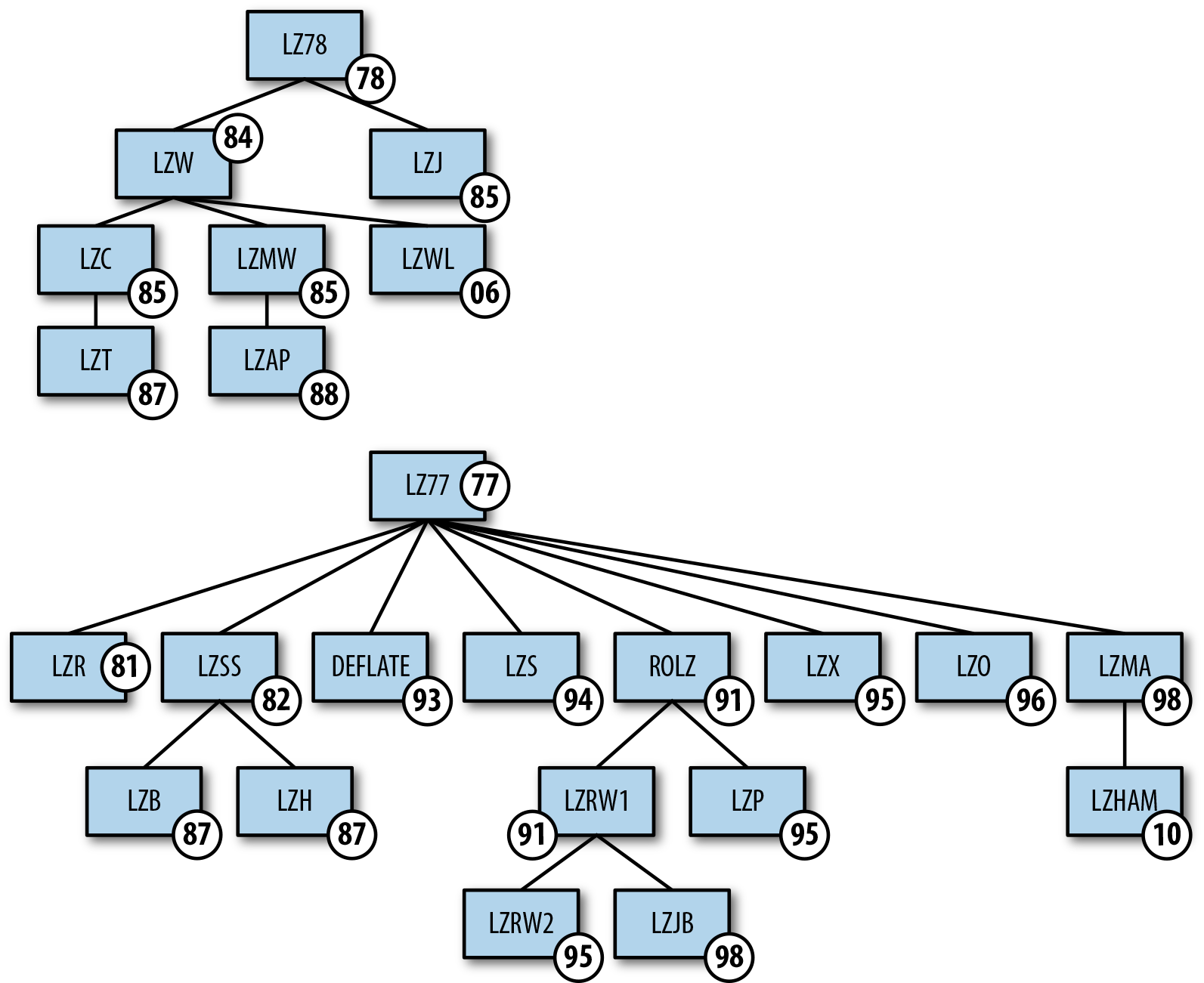
Figure 7-13. A lineage of the LZ77 and LZ78 algorithms that shows the variants and the years they were created.
LZSS
The main difference between LZ77 and LZSS is that in LZ77 the dictionary reference could actually be longer than the string it is replacing. In LZSS, such references are omitted, if the length of the string is less than the “break even” point. Furthermore, LZSS uses one-bit flags to indicate whether the next chunk of data is a literal (byte) or a reference to an offset-length pair.
Many popular archivers like PKZip, ARJ, RAR, ZOO, and LHarc used LZSS as their primary compression algorithm. And as a nostalgia moment: The Game Boy Advance BIOS had built-in functionality to decode a modified LZSS format for patching and so on.
LZW (Lempel–Ziv–Welch)
LZW was published in 1984 by Terry Welch and builds on the idea of the LZ78 algorithm. Here’s how it works:
-
LZW initializes a dictionary with all the possible input characters, as well as clear and stop codes, if they’re used.
-
The algorithm scans through the input string for successively longer substrings until it finds one that is not in the dictionary.
-
When such a string is found, the index for the string without the last character (i.e., the longest substring that is in the dictionary) is retrieved from the dictionary and sent to output.
-
The new string (now including the last character) is added to the dictionary.
-
And the same last input character is then used as the starting point to scan for the next substring.
In this way, successively longer strings are registered in the dictionary and made available for subsequent encoding as single output values. The algorithm works best on data with repeated patterns, because the initial parts of a message will see little compression. As the message grows, however, the compression ratio tends asymptotically to the maximum.
LZW compression became the first widely used universal data compression method on computers. LZW was used in the public-domain program “compress”, which became a more or less standard utility in Unix systems circa 1986. It has since disappeared from many distributions, both because it infringed the LZW patent and because gzip produced better compression ratios using the LZ77-based DEFLATE algorithm.
1 Seriously though, Peter Elias had like 30+ VLCs credited to him.
2 If you wonder why this made-up table doesn’t add up to 1, it’s because of rounding errors. 1/L is 16.66666....
3 Or perhaps more specifically, statistical compressors just accept whatever symbols you throw at them. Dictionary transforms take a given set of symbols and redefine what symbols to use to produce lower entropy for the stream.
4 We’re using the terms “letter” and “word” here to mean “single symbol” and “multiple adjacent symbols,” respectively. To be clear, you can use dictionary transforms on any type of data, not just text.
5 It’s worth noting that in the original LZ77 and LZ78 papers, the token was a triplet, where the third value was the next symbol in the look-ahead stream, which helped with recovery and processing during decoding. Most modern variants of LZ have done away with the need for this third value, so we generally ignore it in the description.
6 As the authors, this is our book, so yeah…wins all around.