Table of Contents for
Understanding Compression
 Understanding Compression
Published by
O'Reilly Media, Inc., 2016
Understanding Compression
Published by
O'Reilly Media, Inc., 2016
- Cover
- nav
- Understanding Compression
- Understanding Compression
- section
- Foreword
- Preface
- 1. Let’s Not Be Boring
- 2. Do Not Skip This Chapter
- 3. Breaking Entropy
- 4. Variable-Length Codes
- 5. Statistical Encoding
- 6. Adaptive Statistical Encoding
- 7. Dictionary Transforms
- 8. Contextual Data Transforms
- 9. Data Modeling
- 10. Switching Gears
- 11. Evaluating Compression
- 12. Compressing Image Data Types
- 13. Serialized Data
- 14. Lossy Data Compression
- 15. Making the World a Little Smaller
- Glossary of Compression Words
- Index
- About the Authors
- Colophon
Chapter 5. Statistical Encoding
Statistically Compressing to Entropy
A variable-length code (VLC) takes a given symbol from your input stream and assigns it a codeword that has a variable number of bits. When you apply this to a long-enough data set, you end up with an average bit-stream length that is close to the entropy of the data set—as long as the probability of your symbol distribution matches the probability table of the encoding scheme you used to build your VLC.
But let’s clear something up: apart from a few situations, the VLCs discussed in Chapter 4 aren’t used much in the mainstream compression world. As we mentioned in that chapter, each code is built making different assumptions about the statistical probabilities of each symbol.
Consider the chaos of using these VLCs in the real world: you’re given an arbitrary data set, and you need to pick the best VLC to encode it, such that the final stream is close to the entropy size. Picking the wrong code for your data set can be disastrous, as you might end up with a compressed data stream that is bigger than the original!
So, you’d need to calculate your stream’s symbol probabilities and then test against all the known VLC codes to determine which one best matches the symbol distribution for your data set. And even then, there’s a chance that your data set might have a probability distribution that doesn’t match exactly with an existing VLC.1
The answer to this is a class of algorithms called statistical encoders, which, instead of mapping a specific integer to a specific codeword, take the probability of your set and use that to define new, unique variable-length codewords for your output stream. The result is that, given any input data, you can uniquely construct a custom set of codewords for it, rather than trying to match an existing VLC.
A more accurate way to describe these algorithms might be that “they excel at using the symbol probability in a data set to encode it as close to entropy as possible.”
Huffman Coding
After all that heavy talk about symbol probabilities that match specific distribution patterns, we now return to real life and, yes, sticky notes. If you do all the tedious work and the probability distribution of symbols in your data stream matches up with any good existing compression algorithm, and there are hundreds of these, you are in luck.
But what if not?
Well, that’s when you need to build your very own. And to produce small, custom VLCs for a given data set, you need an algorithm that takes a list of probabilities and produces codewords.
Enter Huffman coding.
Huffman coding is probably the most straightforward and best-known way to build custom VLCs. Given a set of symbols and their frequencies of occurrence, the method constructs a set of variable-length codewords with the shortest average length for the symbols. It works by setting up a decision tree where the data is sorted and then (we’re almost back to 20 Questions again!) you record the yes/no decisions that get you down the “branches” of the tree to the “leaves”—the individual symbol you’re looking for.
Building a Huffman Tree
In summary, Huffman discovered that if he used a binary tree, he could use the probabilities from the symbol table alongside the branches of the binary tree to create an optimal binary code.
Here’s a tiny—and incomplete—example table:
|
Symbol |
Frequency of occurrence |
|---|---|
|
A |
4 |
|
B |
1 |
|
C |
1 |
So, let’s put these on sticky notes, sort them by probability, and call them the leaves of the binary Huffman tree that we are going to build from the bottom up (see Figure 5-1).
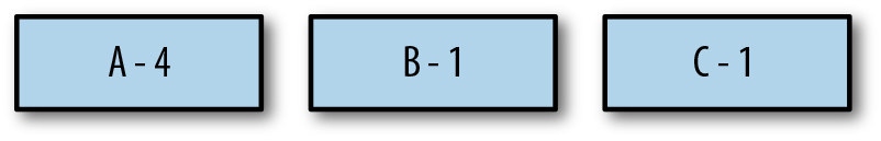
Figure 5-1. The starter nodes sorted by their frequency of occurrence.
First, take the two symbols with the smallest probabilities, move them one level deeper, and create a parent that is a combination of the two symbols and their probabilities, as depicted in Figure 5-2.
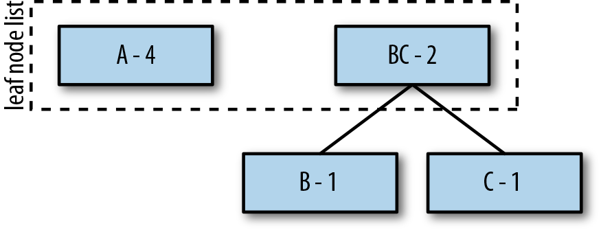
Figure 5-2. Creating a combined parent node for B and C.
Second, repeat this process for the remaining A and combine it with BC to create the new root ABC, which represents our complete set of symbols (see Figure 5-3).
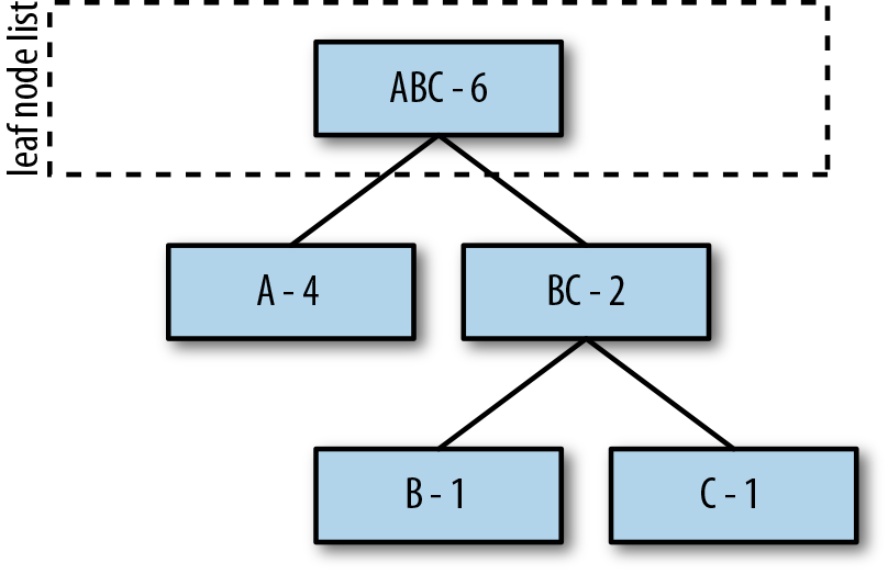
Figure 5-3. Combining A and BC to create the ABC root tree.
Generating Codewords
To set up the tree for generating codewords, assign 0s to all left branches, and 1s to all right branches (Figure 5-4).
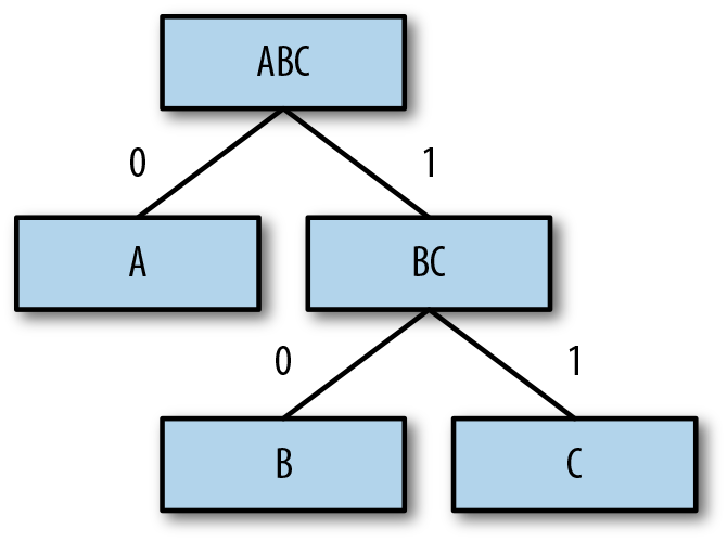
Figure 5-4. Assigning 0s and 1s to the branches.
Finally, to find a code for a given symbol/leaf node, “walk the tree” from the top down,2 and line up the 1s and 0s from most significant bit (MSB) to least significant bit (LSB)—that is, left to right.
For example, to determine the code for B, start at the root, traverse to the right (1), then to the left (0), resulting in 10 as the encoded representation (Figure 5-5).
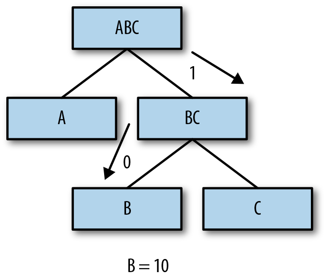
Figure 5-5. Walking the tree to find B’s code.
Finally, repeat this same process for all the remaining symbols/leaves of the tree (Figure 5-6).
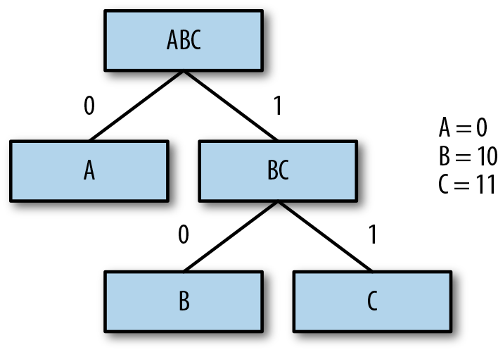
Figure 5-6. Codes for all symbols (leaf nodes) in the tree.
Encoding and Decoding
Congratulations! You now have constructed a VLC assignment for your unique data set, which you can use to encode your data. Walk through the input stream, and for each symbol, write the appropriate codeword to the output.
As with other VLCs, for decoding purposes, you need to transfer the symbol-to-codeword table along with your compressed content and mirror the standard VLC decoding process
Because creating the tree takes more “effort” (uses compute resources) than passing the symbol-to-codeword table (increases data stream size), you should always prepend your data stream with the codeword table, not re-create it at the destination.3
Practical Implementations
Folks have done a crazy amount of amazing analysis on Huffman codes over the past 50 years or so, and have come up with variants to ensure that they operate within some performance or memory threshold, or produce various codes that are skewed toward a specific probability. Entire books have been written about this algorithm and its complexity and optimizations.
But that’s all we’re going to say about it—you’ve got enough of the mechanics to understand how your data is interacting with algorithms when you begin to try them.
Arithmetic Coding
The Huffman method is simple, efficient, and produces the best codes for individual data symbols. However, it doesn’t always produce the most effective codewords for a given set.
In fact, the only case for which Huffman produces ideal VLCs (codes whose average size equals the entropy) is when the symbols occur at probabilities that are negative powers of 2 (i.e., numbers such as 1/2, 1/4, or 1/8). This is because the Huffman method assigns a codeword with an integer number of bits to each symbol in the given symbol set.
Information theory shows that a symbol with probability 0.4 should ideally be assigned a 1.32-bit code, because −log2(0.4) ≈ 1.32. The Huffman method, however, assigns such a symbol a code of 1 or 2 bits.
Sadly, as long as the number of bits we assign to a codeword are integer-based, there will always be a bloated difference between the number of encoded bits and the actual bits required by entropy. So, to fix that, we must move away from assigning integer-based codewords to symbols at a 1:1 ratio.
This is where arithmetic coding comes in. Rather than assigning codewords to symbols in a 1:1 fashion, this algorithm transforms the entire input stream from a set of symbols to one (excessively long) numeric value, whose log2 representation is closer to the true value of entropy for the stream.
The magic of arithmetic compression is a transform that it applies to the source data in order to create a single output number, which takes fewer bits to represent than the source data itself.
Finding the Right Number
Arithmetic coding works by transforming a single string into a number that requires fewer bits to represent than the original string. For example, “TOBEORNOT” could be represented by 2367126, whose ceil(–log2(236712)) = 18 bits. Compare this with the ASCII version of “TOBEORNOT,” which sits at 56 bits.
But this isn’t as easy as just picking a number at random, as we did earlier. Arithmetic coding goes through a complex process of calculating this number from an input stream. The trick is that choosing the number is actually a modification on the binary search algorithm that we introduced in Chapter 2 (you know, the chapter you were not supposed to skip).
If you recall from that chapter, you can use a binary search to output 0/1 bits to catalog the search’s no/yes decision process as we were checking whether a number fit into one of two spaces against a pivot value. But what if we had four spaces? Each decision would then output 2 bits (for one-fourth of the number range, respectively). Still makes pretty good sense, right?
Arithmetic coding kinda works along this path, but with some serious modifications.
Arithmetic coding creates a number space [0,1)7 and subdivides it based on the probability of symbols in the data stream. So, “A” would be given [0,0.25) if its probability were 25%, and B, with a probability of 10%, would then be given [0.25,0.35), and so on, as shown here:
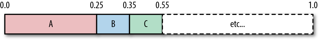
When the encoder reads a symbol, it finds the range for that symbol. For example, if A were read, the range [0.0,0.25) would be used. After a symbol is read, the encoder will subdivide that symbol range and assign new range values for symbols proportionally.
For example, if our stream provided three A symbols in a row, the encoder would subdivide the A range three times, as illustrated here:
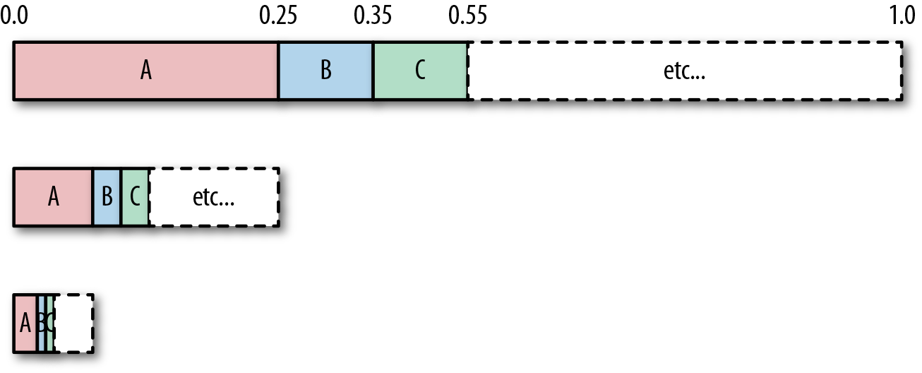
Basically, each symbol recursively divides its range until we reach the end of the input stream. After that’s done, we have a final range of values, such as [0.253212, 0.25421). The number you output, is a value in this range. So for our example, for an input string of AAA, the output could be anything in the range [0,0.015625).
Encoding
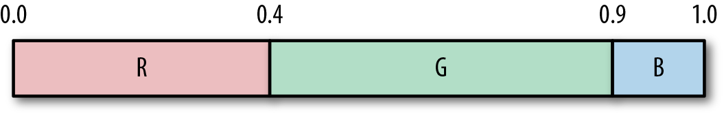
Let’s encode a complete example with three symbols, R, G, and B, with respective probabilities of 0.4, 0.5, and 0.1. We assign them ranges in the interval [0,1) according to their probability, as shown in the following table (note that the entropy of this table is 1.36):
| Symbol | Probability | Interval |
|---|---|---|
|
R |
0.4 |
[0,0.4) |
|
G |
0.5 |
[0.4,0.9) |
|
B |
0.1 |
[0.9,1) |
The following diagram shows the same information represented in number-line form of the ranges for three symbols, R, G, and B:

Using this probability setup, let’s encode the string “GGB.”
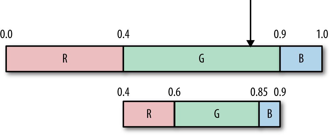
The first symbol we read from the input stream is “G.” Because the interval of G, according to our table, is [0,4,0.9), we subdivide the number space between the values of 0.4 and 0.9 according to probabilities, which gives us a new range of intervals, as shown in the updated figure and table that follow.
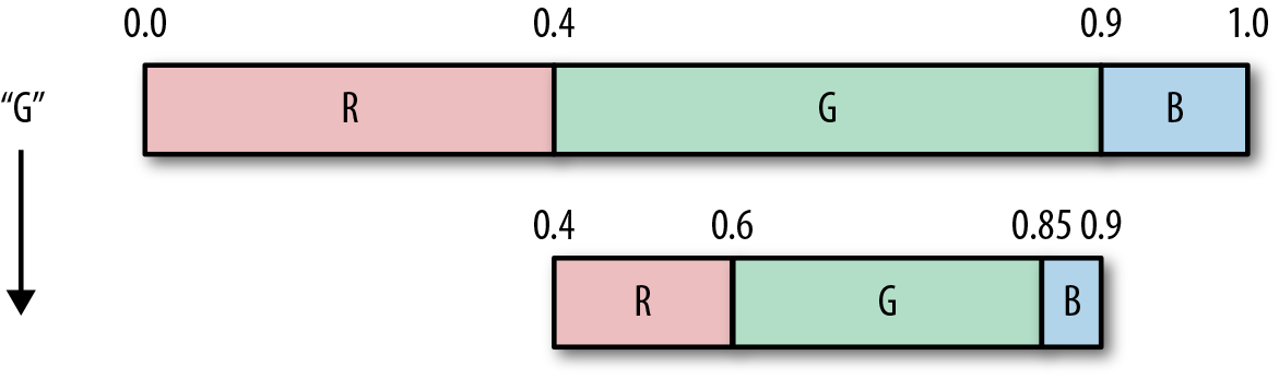
| Symbol | Probability | Updated interval |
|---|---|---|
|
R |
0.4 |
[0.4,0.6) |
|
G |
0.5 |
[0.6,0.85) |
|
B |
0.1 |
[0.85,0.9) |
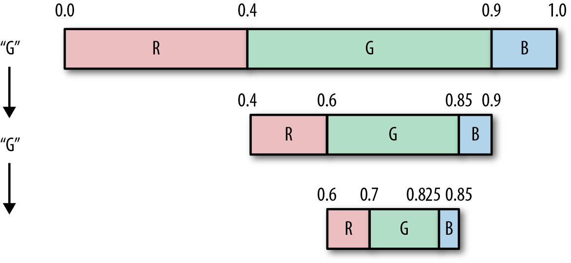
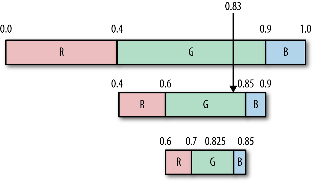
We now read the second symbol from the input stream. It’s another G, so we again subdivide the G range of numbers, which is between 0.6 and 0.85, and update the intervals as shown in the following figure and the table.
| Symbol | Probability | Updated interval |
|---|---|---|
|
R |
0.4 |
[0.6,0.7) |
|
G |
0.5 |
[0.7,0.825) |
|
B |
0.1 |
[0.825,0.85) |
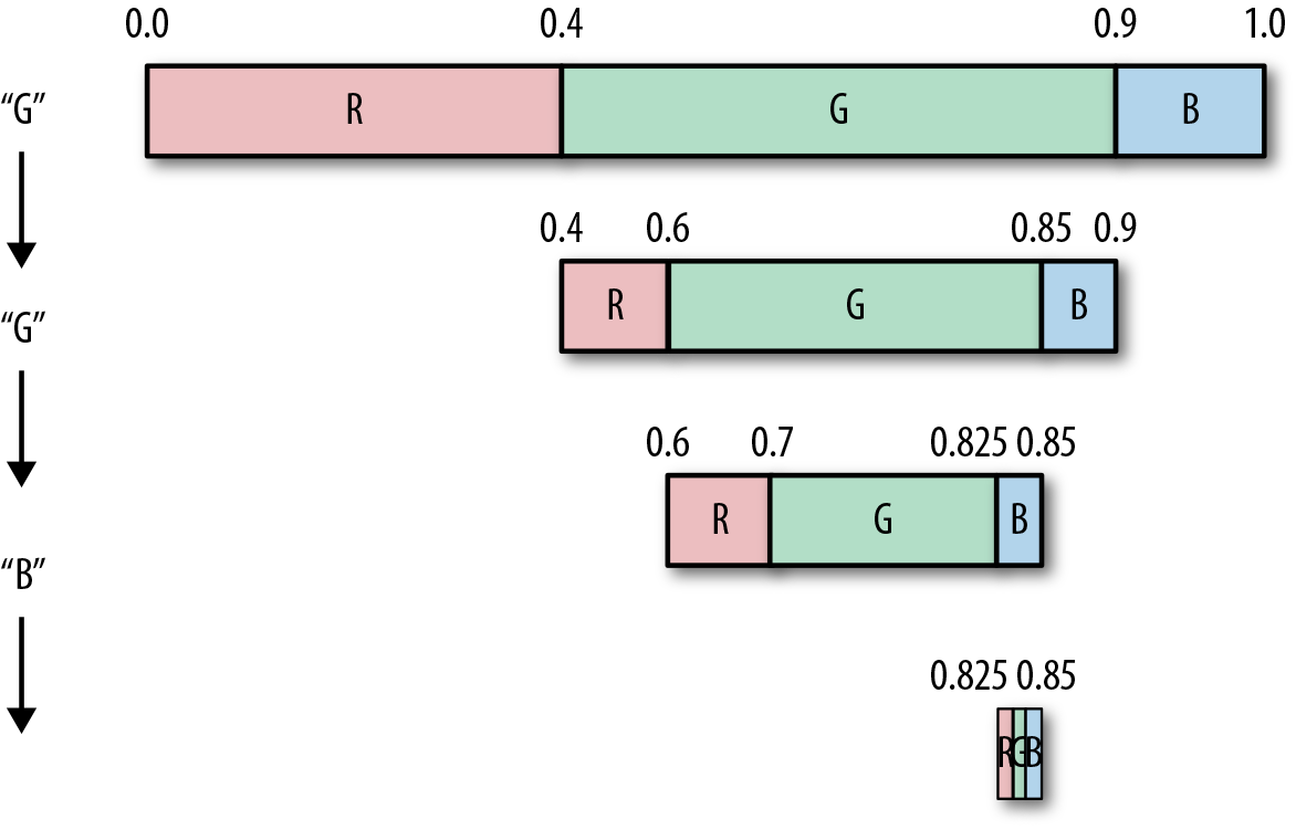
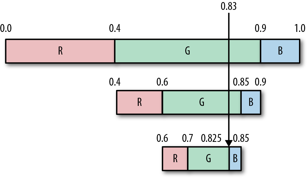
And finally, we read and subdivide again for the letter B, and update the figure and table once more.
| Symbol | Probability | Updated interval |
|---|---|---|
|
R |
0.4 |
[0.825,0.835) |
|
G |
0.5 |
[0.835,0.8475) |
|
B |
0.1 |
[0.8475,0.85) |
Congratulations! You just arithmetically encoded a stream!
Picking the Right Output Value
So, we’ve subdivided the range intervals, but what number do we output as the final result?
Our final interval for B is [0.825,0.85), and any number from that range will serve the purpose of letting us reconstruct the original string, giving us some choices between 0.825 and 0.849999.... This being a book about compression, we want to use the number that we can represent with the fewest bits (and as close to our 1.36 bits entropy goal) as possible.
The number in this range that requires the fewest bit is 0.83.
Finally, because the decoder “knows” that this is a floating-point number, we can drop the leading 0 for additional savings and end up with 83, which with log2(83) = 7 bits, gives us 1.42 bits per symbol, which is almost at entropy.
Decoding
Decoding from this final number is pretty straightforward—basically the encoding process in reverse. Just as with encoding, we begin by creating the segmented range between [0,1) based on the probabilities, as demonstrated here:
We then take our input value, 83, add the leading “0” to get 0.83, and find which interval it falls into. We output the symbol associated with that interval.
In our case, 0.83 falls in the range 0.4,0.9, giving us the value G to output.
We then subdivide the G space according to the probabilities (same as when we were encoding).
To get our second symbol, we repeat the process. Our input value is still 0.83, which falls (again) in G’s range, so we output another G, and subdivide again, as shown here:
Continuing one more time, 0.83 falls in the range 0.825,0.85, which is the range for the symbol B, so we output B.
This gives us our final decoded stream as GGB.
Pretty nifty, eh? Our decoding process basically works by drawing a line through each recursive space and outputting whatever symbol we land in at that time.
Practical Implementations
The adoption and dominance of arithmetic coding since its patent expiration in the 2000s has led to a plethora of topics that relate to practical implementations of this algorithm. More impressive is how many of them have been modified for specific codecs, such as the binary-only versions used by JPG and H.264 codecs. Those lossy compression methods are out of scope for this book, but there are plenty of resources out there if you’d like to investigate more.
Asymmetric Numeral Systems
After a 40-year battle between Huffman and arithmetic encodings, it would seem as though both might have been usurped by a brand new class of statistical encoder.
In 2007, Jarek Duda presented a new information theory concept called asymmetric numeral systems (ANS) that had direct relations to data compression. Effectively, ANS is a new approach to accurate entropy coding, which can get arbitrarily close to optimal Shannon entropy, provides compression ratios similar to arithmetic coding, and has performance similar to Huffman coding.
Although Jarek Duda’s papers detail a lot of cool mathematical revelations, you can apply the algorithm itself much like other statistical encoders:8
- A numerical space is subdivided based on symbol frequencies.
- A table is created, which maps subspaces to discrete integer values.
- Each symbol is processed by reading and responding to values in the table.
- Variable bits are written to the output stream.
The two parts that are unique to this algorithm are in step 2 (the table) and step 4 (variable bits).
So, let’s take a look at those more closely.
Encoding and Decoding Using a Transform Table
The tANS variant of ANS works by moving around a table of values.
As an example, let’s just assume that you’re given the table that follows. Ignore how we’ve created it, we’ll get to table creation in a moment.
| State/row | A | B | C |
|---|---|---|---|
|
1 |
2 |
3 |
5 |
|
2 |
4 |
6 |
10 |
|
3 |
7 |
8 |
15 |
|
4 |
9 |
11 |
20 |
|
5 |
12 |
14 |
25 |
|
6 |
13 |
17 |
30 |
|
7 |
16 |
21 |
|
|
8 |
18 |
22 |
|
|
9 |
19 |
26 |
|
|
10 |
23 |
28 |
|
|
11 |
24 |
||
|
12 |
27 |
||
|
13 |
29 |
||
|
14 |
31 |
Given the preceding table, let’s walk through how to encode the input string BAA:
-
Given an input stream BAA, we begin with a pair of [row index, input symbol], which is [1,B].9
-
We use this pair to reference a location in the table from which to read our next value. We grab the value at cell [1,B] in the table, which is 3, and make that our new row index for [3,?].
-
To get the column index, we then read the next symbol, which is A, completing the new table index [3,A].
-
Again, we grab the value at that cell in the table, which is 7.
-
We read the next symbol, which is also A, we end up with [7,A].
-
And the value at that index is 16.
-
We can continue forward with this until we hit the end of the table (or the end of the string).
-
The transform of this table takes BAA and results in [3,7,16].
Decoding works in the exact opposite way.
-
We begin with the last value, 16.
-
We then search the entire table and find that 16 sits at row 7, column A.
-
We output A as our symbol and 7 becomes the new current value.
-
We search the table again and find that 7 is at row 3, column A.
-
We output A, again, and set 3 as our new value.
-
When we search for our last 3, we see that it’s at row 1, column B. Because we’re in row 1, we know we can’t move further, so we’re done decoding.
-
The decoded stream is [A,A,B] because we were decoding the list from back to front.
-
Our last step is to reverse to get to the original BAA.
You can see that this table lets us encode an input string and decode it properly, given a nifty way to move around it.
Creating the Reference Table
The core of this algorithm is the magical reference table, which makes it possible for these types of transforms to occur. The table itself is created by first assigning each symbol a column in the table, such that the symbols are sorted by probability, left to right from highest to lowest.
In the previous table, the symbols A, B, C have the probabilities P([A,B,C]) = [0.45,0.35,0.2], and are each assigned a column of the table.
From here, we must fill in values into the table, adhering to a few specific properties:
-
Every value in the table is unique (no repeats)
-
Numbers in each column are sorted from lowest to highest
-
Numbers in every row are larger than the number (index) of that row
If you can adhere to these principles, the encoding/decoding transform that we’ve shown should work just fine. But for tANS to become a true entropy encoder, there are two more properties that we must consider:
- Determining the number of values in a column
- The number of values in a column is equal to the probability of the column-symbol, multiplied by maxVal.10
- Determining the numbers in each row
- Numbers in a row are selected to align with the probability of occurrence for a symbol, such that if we divide the row-number by a value in a column, the resulting value is (roughly) equal to the probability of that column’s symbol.
Let’s take a closer look at these properties for our example.
The first property is somewhat straightforward. The largest value in the table is maxVal = 31. In accordance with the property, we subdivide the space of maxVal = 31, assigning P(s) * maxVal numbers to each symbol-column. For our example:
- B has P(B) = 0.35, which results in a column that is floor(0.35 * 31) = 10 elements high.
- The same goes for C (0.2 * 31 = 6).
- However, the most-probable symbol, in the leftmost column A, has P(A) * maxVal + 1 = 0.45 * 31 + 1 = 14 rows. That’s because the most probable symbol adds an extra row for the maxVal.
This has the effect of subdividing the maxVal space, giving slots for each symbol, equal to its probability.11
The second property defines that values in a row can be calculated by multiplying the row number by the probability of each symbol.
For our example table, the probabilities for the symbols S = [A,B,C] are P(S) = [0.45,0.35,0.2], and picking a row, say row 5, the values are 12, 14, 25.
When we divide those values by the row index, we get a result that’s pretty close to the symbol probabilities: [ 5 / 12, 5 / 14 , 5 / 25] = [0.41666.,0.357,0.2 ] ~= P(S).
This second property must remain true for all rows. You can see that for column A, each row has a value that’s about right with regard to P(A) = 0.45.
| Row # | P(A) | Row #/P(A) |
Actual table value |
Row #/value |
|---|---|---|---|---|
|
1 |
0.45 |
2.2223… |
2 |
0.5 |
|
2 |
0.45 |
4.4444… |
4 |
0.5 |
|
3 |
0.45 |
6.6666… |
7 |
0.42 |
|
4 |
0.45 |
8.8888… |
9 |
0.444… |
|
5 |
0.45 |
11.1111… |
12 |
0.416… |
So, why is there sometimes a discrepancy between the assigned table value and the numerically calculated table value? It’s to avoid collisions.
Each value in the table must be unique. However, because we are rounding numbers up and down, we can end up with collisions at a few spots. For example, 1 / P(C) = 5, whereas 2 / P(B) = 5.714.
We resolve collisions by iterating forward to find the next highest value that is not yet used in the table. For example, in the case of assigning a symbol to column B, for row 2 we can’t use the value 5 (because it’s already used in row 1), so we try the next greater value, 6, which hasn’t been used in the table yet, and assign12 that value.
By adhering to these two properties, you can create the entire preceding table that will properly encode/decode values and compress your data.
Choosing a maxVal
Choosing maxVal directly affects your compression output, which is directly related to the amount of integer precision that your encoding allows.
The goal, therefore, is to assign each symbol a subspace whose size matches the probability of the symbol itself. Now, if the encoding process and table were computed in floating-point space, this wouldn’t be that big of a deal: simply assign each symbol a space equal to its frequency. However, our encode/decode works with integers. As such, we need to create an integer space of some size (between 2 and maxVal) such that we can assign subranges of it to each symbol without running into precision problems.
Suppose that your data set contains 28 unique symbols. At the bare minimum, you then need LOG2(28) = 5 bits, space size, giving you a maxVal of 25 - 1 = 31.
However, because not every symbol is equally probable, this doesn’t give us enough space to assign different symbols different space sizes. To accommodate, this we need to increase our number of bits.
As such, choosing a maxVal should be a function of the minimum number of bits you need, plus a few extra bits to help with precision:
numPrecisionBits = LOG2(numSymbols) + magicExtraBits
maxVal = (2numPrecisionBits) - 1
Where magicExtraBits is some value between 2 and 8, or whatever works for your data set. The number of magicExtraBits, as we will show in a moment, trades off quality for processing time; the higher the value, the better compression but the longer it takes to compress.
Using ANS for Compression
We previously identified how to move around our reference table; however, the output didn’t result in statistical compression. To achieve compression, we need to tweak our algorithm just a tad:
-
First, instead of starting with row 1, our starting state/row is going to be maxVal.
-
Second, for each symbol we read from the stream:
-
Set targetRow to the column height for that symbol.
-
Bitshift the state value right until it is smaller than the targetRow.
-
Each bit that is dropped from state during the shift, should be output to our encoded bitstream.
-
Let’s walk through an example encoding of the string “ABAC”, given the above modifications and the table we previously presented:
-
Because the state = maxVal = 31 (binary 11111), that is what we start with.
-
Read the first symbol, which is A, giving us [31,A], and setting targetRow to 14.
-
Because 31 > 14, we start shifting and outputting bits.
-
We shift state right once, to 1111, truncating the rightmost 1 to our output stream→1.
-
State is now 15, which is still larger than 14; thus, we shift right again, making state 111 and outputting another 1 bit to the output stream. →1
-
State is now 7, and we’ve truncated and written out two bits (11).
-
-
We now assign state to the table value at [7,A], which is 16 (binary 10000).
-
Read the next symbol, which is B, resulting in [16,B], and setting targetRow to 10.
-
Because 16 > 10, we start shifting and outputting bits.
-
We shift 16 right once to set state = 8 (binary 1000), emitting a 0 to the output. →0
-
Because 8 <10, we can move to the next symbol.
-
-
We set state to the table value at [8,B], which is 22 (binary 10110).
-
Read the next symbol, which is A, resulting in [22,A], and setting targetRow to 14.
-
Because 22 > 14, we shift and output bits. We shift right to get state = 1011, emitting 0. →0
-
We set state to the table value at [11,A], which is 24 (binary 11000).
-
Read the next symbol, which is C, resulting in [24,C], and targetRow to 6.
-
Because 24 > 6, we start shifting and outputting bits. We shift twice to get state = 110, emitting 00. →0 0
-
We set state to the table value at [6,C], which is 30 (11110).
-
Because our stream is now empty, we output our state value (11110) to the stream. →11110
-
Our final stream is thus: 11000011110 and 11 bits long. Plus the bits taken up by the symbol probabilities table.
Decoding Example
Decoding works in the opposite order:
-
Read in our frequency data from the compressed stream.
-
Create the table from the symbol frequency information.
-
Read a value from the stream.
-
Find its location in the table.
-
Output the column as the symbol.
-
Make value = row.
-
Read in some new bits.
It’s worth noting that in this example our maxVal = 31, or 5 bits of precision.
After creating the table, we work through our encoded 11000011110 stream backward as follows:
-
Working with 5 bits for our state targeted, read the last 5 bits 11110(30) of the stream.
-
We find the only number 30 in the table at location [C,6].
-
Output the symbol C.
-
6 or 110 is only 3 bits, so we need to read 2 more from the stream (always try to make 5 bits).
-
Read the last 2 bits, 00, and append them to 110, resulting in 11000 24
-
Find the only location of 24 in the table at [A,11].
-
Output the symbol A.
-
11 (binary 1011) is only 4 bits, so read 1 more bit from the stream, giving you 10110 (22).
-
Find 22 in the table at [B,8].
-
Output the symbol B.
-
8 (binary 1000) is only 4 bits, so read 1 more, giving you 10000 (16).
-
Find 16 in the table at [A,7].
-
Output the symbol A.
-
7 (binary 111) is only 3 bits, so read 2 more, giving you 11111(31).
-
Because this value now equals our maxValue (11111), we know this to be the end-of-message marker, so we quit decoding.
-
We reverse the string and have returned to ABAC.
So Where Does the Compression Come From?
Compression comes from the bit-wise output.
Because the least probable symbols have shorter columns, the valid row values are farther removed (in bit distance) from the max-symbol. Therefore, more right-shifts are required to get to the lower row indexes, which means more bits are pushed to the stream for each iteration. So, less probable symbols result in more bits being output to the final stream.
As we mentioned previously, giving more bits produces a higher precision for your space (and thus, a larger maxVal). This causes the values in the reference table to have fewer precision collisions, because the larger space allows for integers to more closely match the value given by P(s) * maxVal. Recall that collisions in the table result in linearly searching for a larger value that hasn’t been used yet. When encoding, this difference between the computed value and the actual value can result in more bit-shifts to get the state value below the target row value. When precision is high, there are fewer collisions, producing less bloat per value and fewer bits being shifted to the output stream.
The downside, though, is that larger precision produces a larger reference table, which takes significant time to create and significant amounts of memory to hold. So ensure that you find the right trade-off between performance and memory for your particular implementation.
Practical Compression: Which Statistical Algorithm Do I Choose?
So, you’ve got some awesome data set, and three awesome algorithms to apply statistical compression to them. Which one do you choose?
This is a common problem, and for the majority of the past 20 years, there’s been a massive nerd-fight going on in the compression world between Huffman and arithmetic coding. This debate first came to light in 1993, when Bookstein and Klein published a paper called “Is Huffman Coding Dead?”
Although it’s been more than 20 years since that paper was released, the arguments are still held strongly by both sides of the debate.
Because computers are getting faster and faster (and the patent on arithmetic compression has expired), arithmetic compression has become the more dominantly implemented version. It has taken over in most multimedia encoders, and is even being implemented into hardware effectively.
But ANS has changed all that. In its short time in the world of compression, it has already begun to take over the majority of positions held by Huffman and arithmetic encoders for the past 20 years.
For example, the ZHuff, LZTurbo, LZA, Oodle and LZNA compressors have already made the move over to ANS. Given its speed and performance, it seems only a matter of time before it will become the dominant form of encoding. In fact, in 2013, a more performance-focused version of the algorithm called Finite State Entropy (FSE), which only uses additions, masks, and shifts, came onto the scene, making ANS even more attractive for developers. It’s so powerful, that a Gzip-variant, dubbed LZFSE, was unveiled in 2015 as a core API in Apple’s next iOS release.
The road forward seems pretty clear at this point: ANS and FSE might usher the end of the decades that Huffman and arithmetic have enjoyed on the top of the charts.
1 Of course, where explicit VLCs are used in modern compressors is where the probabilities of the transformed input stream is pretty known. As such, the encoder and decoder can just agree on what VLC to use, and move forward.
2 Guilty admission: this isn’t entirely accurate. The traditional Huffman code works by traversing bottom up (as opposed to the Shannon–Fano method, which works from the top down). For programmers: in practice, we’ve found that traversing top-down yields a more efficient code-wise implementation, because it’s simpler to keep child pointers and tree traversals that way.
3 Balancing data transmission with computing resources is a theme we’ll return to at the end of this book; it’s a recurrent challenge.
4 He was also one of the pioneers in the field of mathematical origami, the wonders of which you can begin exploring with Robert Lang’s TED talk “The Math and Magic of Origami”.
5 Inna Pivkina, “Discovery of Huffman Codes”.
6 It actually isn’t. This is just an example number to show you the general steps.
7 The [0,1) notation indicates that the number 0 is included in the range, and 1 is not, making the range 0 through 0.99999…, with as many 9s as you need.
8 Especially the tANS variant, which is designed to be a direct replacement to Huffman encoding. See the paper “The Use of Asymmetric Numeral Systems as an Accurate Replacement for Huffman Coding” or “Asymmetric Numeral Systems: Entropy Coding Combining Speed of Huffman Coding with Compression Rate of Arithmetic Coding”.
9 Worth noting that 1 is always the initial state.
10 We haven’t talked about maxVal yet. We’ll get into choosing the proper maxVal in a moment.
11 Note that if you’re creating this as a full 2D table (rather than letting the height of each column be variable), you’ll need to insert some value in the column positions greater than its column height (–1 or something) to signify that those cells are empty/invalid.
12 With respect to performance, there’s a bunch of different ways to accomplish this type of marking of used variables. We suggest checking out the “bingo board” method by Andrew Polar.