Table of Contents for
Linux Network Administrator's Guide, Second Edition
 Linux Network Administrator's Guide, Second Edition
Published by
O'Reilly Media, Inc., 2000
Linux Network Administrator's Guide, Second Edition
Published by
O'Reilly Media, Inc., 2000
- Cover
- Linux Network Administrator’s Guide, 2nd Edition
- Preface
- Sources of Information
- File System Standards
- Standard Linux Base
- About This Book
- The Official Printed Version
- Overview
- Conventions Used in This Book
- Submitting Changes
- Acknowledgments
- 1. Introduction to Networking
- TCP/IP Networks
- UUCP Networks
- Linux Networking
- Maintaining Your System
- 2. Issues of TCP/IP Networking
- IP Addresses
- Address Resolution
- IP Routing
- The Internet Control Message Protocol
- Resolving Host Names
- 3. Configuring the Networking Hardware
- A Tour of Linux Network Devices
- Ethernet Installation
- The PLIP Driver
- The PPP and SLIP Drivers
- Other Network Types
- 4. Configuring the Serial Hardware
- Introduction to Serial Devices
- Accessing Serial Devices
- Serial Hardware
- Using the Configuration Utilities
- Serial Devices and the login: Prompt
- 5. Configuring TCP/IP Networking
- Installing the Binaries
- Setting the Hostname
- Assigning IP Addresses
- Creating Subnets
- Writing hosts and networks Files
- Interface Configuration for IP
- All About ifconfig
- The netstat Command
- Checking the ARP Tables
- 6. Name Service and Resolver Configuration
- How DNS Works
- Running named
- 7. Serial Line IP
- SLIP Operation
- Dealing with Private IP Networks
- Using dip
- Running in Server Mode
- 8. The Point-to-Point Protocol
- Running pppd
- Using Options Files
- Using chat to Automate Dialing
- IP Configuration Options
- Link Control Options
- General Security Considerations
- Authentication with PPP
- Debugging Your PPP Setup
- More Advanced PPP Configurations
- 9. TCP/IP Firewall
- What Is a Firewall?
- What Is IP Filtering?
- Setting Up Linux for Firewalling
- Three Ways We Can Do Filtering
- Original IP Firewall (2.0 Kernels)
- IP Firewall Chains (2.2 Kernels)
- Netfilter and IP Tables (2.4 Kernels)
- TOS Bit Manipulation
- Testing a Firewall Configuration
- A Sample Firewall Configuration
- 10. IP Accounting
- Configuring IP Accounting
- Using IP Accounting Results
- Resetting the Counters
- Flushing the Ruleset
- Passive Collection of Accounting Data
- 11. IP Masquerade and Network Address Translation
- Configuring the Kernel for IP Masquerade
- Configuring IP Masquerade
- Handling Name Server Lookups
- More About Network Address Translation
- 12. Important Network Features
- The tcpd Access Control Facility
- The Services and Protocols Files
- Remote Procedure Call
- Configuring Remote Login and Execution
- 13. The Network Information System
- NIS Versus NIS+
- The Client Side of NIS
- Running an NIS Server
- NIS Server Security
- Setting Up an NIS Client with GNU libc
- Choosing the Right Maps
- Using the passwd and group Maps
- Using NIS with Shadow Support
- 14. The Network File System
- Mounting an NFS Volume
- The NFS Daemons
- The exports File
- Kernel-Based NFSv2 Server Support
- Kernel-Based NFSv3 Server Support
- 15. IPX and the NCP Filesystem
- IPX and Linux
- Configuring the Kernel for IPX and NCPFS
- Configuring IPX Interfaces
- Configuring an IPX Router
- Mounting a Remote NetWare Volume
- Exploring Some of the Other IPX Tools
- Printing to a NetWare Print Queue
- NetWare Server Emulation
- 16. Managing Taylor UUCP
- UUCP Configuration Files
- Controlling Access to UUCP Features
- Setting Up Your System for Dialing In
- UUCP Low-Level Protocols
- Troubleshooting
- Log Files and Debugging
- 17. Electronic Mail
- How Is Mail Delivered?
- Email Addresses
- How Does Mail Routing Work?
- Configuring elm
- 18. Sendmail
- Installing sendmail
- Overview of Configuration Files
- The sendmail.cf and sendmail.mc Files
- Generating the sendmail.cf File
- Interpreting and Writing Rewrite Rules
- Configuring sendmail Options
- Some Useful sendmail Configurations
- Testing Your Configuration
- Running sendmail
- Tips and Tricks
- 19. Getting Exim Up and Running
- If Your Mail Doesn’t Get Through
- Compiling Exim
- Mail Delivery Modes
- Miscellaneous config Options
- Message Routing and Delivery
- Protecting Against Mail Spam
- UUCP Setup
- 20. Netnews
- What Is Usenet, Anyway?
- How Does Usenet Handle News?
- 21. C News
- Installation
- The sys File
- The active File
- Article Batching
- Expiring News
- Miscellaneous Files
- Control Messages
- C News in an NFS Environment
- Maintenance Tools and Tasks
- 22. NNTP and the nntpd Daemon
- Installing the NNTP Server
- Restricting NNTP Access
- NNTP Authorization
- nntpd Interaction with C News
- 23. Internet News
- Newsreaders and INN
- Installing INN
- Configuring INN: the Basic Setup
- INN Configuration Files
- Running INN
- Managing INN: The ctlinnd Command
- 24. Newsreader Configuration
- trn Configuration
- nn Configuration
- A. Example Network: The Virtual Brewery
- B. Useful Cable Configurations
- A Serial NULL Modem Cable
- C. Linux Network Administrator’s Guide, Second Edition Copyright Information
- 1. Applicability and Definitions
- 2. Verbatim Copying
- 3. Copying in Quantity
- 4. Modifications
- 5. Combining Documents
- 6. Collections of Documents
- 7. Aggregation with Independent Works
- 8. Translation
- 9. Termination
- 10. Future Revisions of this License
- D. SAGE: The System Administrators Guild
- Index
- Colophon
We now take up the question of finding the host that datagrams go to based on the IP address. Different parts of the address are handled in different ways; it is your job to set up the files that indicate how to treat each part.
When you write a letter to someone, you usually put a complete address on the envelope specifying the country, state, and Zip Code. After you put it in the mailbox, the post office will deliver it to its destination: it will be sent to the country indicated, where the national service will dispatch it to the proper state and region. The advantage of this hierarchical scheme is obvious: wherever you post the letter, the local postmaster knows roughly which direction to forward the letter, but the postmaster doesn’t care which way the letter will travel once it reaches its country of destination.
IP networks are structured similarly. The whole Internet consists of a number of proper networks, called autonomous systems. Each system performs routing between its member hosts internally so that the task of delivering a datagram is reduced to finding a path to the destination host’s network. As soon as the datagram is handed to any host on that particular network, further processing is done exclusively by the network itself.
This structure is reflected by splitting IP addresses into a host and network part, as explained previously. By default, the destination network is derived from the network part of the IP address. Thus, hosts with identical IP network numbers should be found within the same network.[15]
It makes sense to offer a similar scheme inside the network, too, since it may consist of a collection of hundreds of smaller networks, with the smallest units being physical networks like Ethernets. Therefore, IP allows you to subdivide an IP network into several subnets.
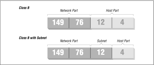
A subnet takes responsibility for delivering datagrams to a certain range of IP addresses. It is an extension of the concept of splitting bit fields, as in the A, B, and C classes. However, the network part is now extended to include some bits from the host part. The number of bits that are interpreted as the subnet number is given by the so-called subnet mask, or netmask. This is a 32-bit number too, which specifies the bit mask for the network part of the IP address.
The campus network of Groucho Marx University is an example of such a network. It has a class B network number of 149.76.0.0, and its netmask is therefore 255.255.0.0.
Internally, GMU’s campus network consists of several smaller networks, such various departments’ LANs. So the range of IP addresses is broken up into 254 subnets, 149.76.1.0 through 149.76.254.0. For example, the department of Theoretical Physics has been assigned 149.76.12.0. The campus backbone is a network in its own right, and is given 149.76.1.0. These subnets share the same IP network number, while the third octet is used to distinguish between them. They will thus use a subnet mask of 255.255.255.0.
Figure 2.1 shows how 149.76.12.4, the address of quark, is interpreted differently when the address is taken as an ordinary class B network and when used with subnetting.
It is worth noting that subnetting (the technique of generating subnets) is only an internal division of the network. Subnets are generated by the network owner (or the administrators). Frequently, subnets are created to reflect existing boundaries, be they physical (between two Ethernets), administrative (between two departments), or geographical (between two locations), and authority over each subnet is delegated to some contact person. However, this structure affects only the network’s internal behavior, and is completely invisible to the outside world.
Subnetting is not only a benefit to the organization; it is frequently a natural consequence of hardware boundaries. The viewpoint of a host on a given physical network, such as an Ethernet, is a very limited one: it can only talk to the host of the network it is on. All other hosts can be accessed only through special-purpose machines called gateways. A gateway is a host that is connected to two or more physical networks simultaneously and is configured to switch packets between them.
Figure 2.2 shows part of the network topology at Groucho Marx University (GMU). Hosts that are on two subnets at the same time are shown with both addresses.
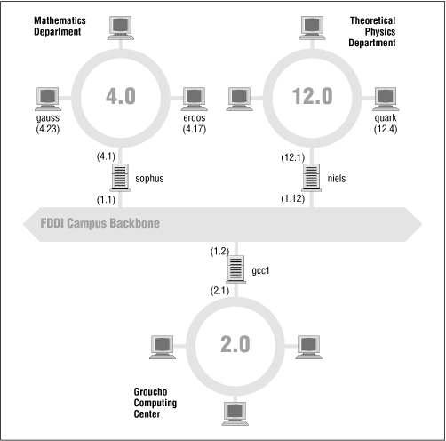
Different physical networks have to belong to different IP networks for IP to be able to recognize if a host is on a local network. For example, the network number 149.76.4.0 is reserved for hosts on the mathematics LAN. When sending a datagram to quark, the network software on erdos immediately sees from the IP address 149.76.12.4 that the destination host is on a different physical network, and therefore can be reached only through a gateway (sophus by default).
sophus itself is connected to two
distinct subnets: the Mathematics department and the campus backbone. It
accesses each through a different interface, eth0 and
fddi0, respectively. Now, what IP address do we assign
it? Should we give it one on subnet
149.76.1.0, or on
149.76.4.0?
The answer is: “both.” sophus has been assigned the address 149.76.1.1 for use on the 149.76.1.0 network and address 149.76.4.1 for use on the 149.76.4.0 network. A gateway must be assigned one IP address for each network it belongs to. These addresses—along with the corresponding netmask—are tied to the interface through which the subnet is accessed. Thus, the interface and address mapping for sophus would look like this:
| Interface | Address | Netmask |
|---|---|---|
eth0
| 149.76.4.1 | 255.255.255.0 |
fddi0
| 149.76.1.1 | 255.255.255.0 |
lo
| 127.0.0.1 | 255.0.0.0 |
The last entry describes the loopback interface lo, which
we talked about earlier.
Generally, you can ignore the subtle difference between attaching an address to a host or its interface. For hosts that are on one network only, like erdos, you would generally refer to the host as having this-and-that IP address, although strictly speaking, it’s the Ethernet interface that has this IP address. The distinction is really important only when you refer to a gateway.
We now focus our attention on how IP chooses a gateway to use to deliver a datagram to a remote network.
We have seen that erdos, when given a datagram for quark, checks the destination address and finds that it is not on the local network. erdos therefore sends the datagram to the default gateway sophus, which is now faced with the same task. sophus recognizes that quark is not on any of the networks it is connected to directly, so it has to find yet another gateway to forward it through. The correct choice would be niels, the gateway to the Physics department. sophus thus needs information to associate a destination network with a suitable gateway.
IP uses a table for this task that associates networks with the gateways by which they may be reached. A catch-all entry (the default route) must generally be supplied too; this is the gateway associated with network 0.0.0.0. All destination addresses match this route, since none of the 32 bits are required to match, and therefore packets to an unknown network are sent through the default route. On sophus, the table might look like this:
| Network | Netmask | Gateway | Interface |
|---|---|---|---|
| 149.76.1.0 | 255.255.255.0 | - |
fddi0
|
| 149.76.2.0 | 255.255.255.0 | 149.76.1.2 |
fddi0
|
| 149.76.3.0 | 255.255.255.0 | 149.76.1.3 |
fddi0
|
| 149.76.4.0 | 255.255.255.0 | - |
eth0
|
| 149.76.5.0 | 255.255.255.0 | 149.76.1.5 |
fddi0
|
| ... | ... | ... | ... |
| 0.0.0.0 | 0.0.0.0 | 149.76.1.2 |
fddi0
|
If you need to use a route to a network that sophus is directly connected to, you don’t need a gateway; the gateway column here contains a hyphen.
The process for identifying whether a particular destination address matches a route is a mathematical operation. The process is quite simple, but it requires an understanding of binary arithmetic and logic: A route matches a destination if the network address logically ANDed with the netmask precisely equals the destination address logically ANDed with the netmask.
Translation: a route matches if the number of bits of the network address specified by the netmask (starting from the left-most bit, the high order bit of byte one of the address) match that same number of bits in the destination address.
When the IP implementation is searching for the best route to a destination, it may find a number of routing entries that match the target address. For example, we know that the default route matches every destination, but datagrams destined for locally attached networks will match their local route, too. How does IP know which route to use? It is here that the netmask plays an important role. While both routes match the destination, one of the routes has a larger netmask than the other. We previously mentioned that the netmask was used to break up our address space into smaller networks. The larger a netmask is, the more specifically a target address is matched; when routing datagrams, we should always choose the route that has the largest netmask. The default route has a netmask of zero bits, and in the configuration presented above, the locally attached networks have a 24-bit netmask. If a datagram matches a locally attached network, it will be routed to the appropriate device in preference to following the default route because the local network route matches with a greater number of bits. The only datagrams that will be routed via the default route are those that don’t match any other route.
You can build routing tables by a variety of means. For small LANs, it is usually most efficient to construct them by hand and feed them to IP using the route command at boot time (see Chapter 5). For larger networks, they are built and adjusted at runtime by routing daemons; these daemons run on central hosts of the network and exchange routing information to compute “optimal” routes between the member networks.
Depending on the size of the network, you’ll need to use different routing protocols. For routing inside autonomous systems (such as the Groucho Marx campus), the internal routing protocols are used. The most prominent one of these is the Routing Information Protocol (RIP), which is implemented by the BSD routed daemon. For routing between autonomous systems, external routing protocols like External Gateway Protocol (EGP) or Border Gateway Protocol (BGP) have to be used; these protocols, including RIP, have been implemented in the University of Cornell’s gated daemon.
We depend on dynamic routing to choose the best route to a destination host or network based on the number of hops. Hops are the gateways a datagram has to pass before reaching a host or network. The shorter a route is, the better RIP rates it. Very long routes with 16 or more hops are regarded as unusable and are discarded.
RIP manages routing information internal to your local network, but you have to run gated on all hosts. At boot time, gated checks for all active network interfaces. If there is more than one active interface (not counting the loopback interface), it assumes the host is switching packets between several networks and will actively exchange and broadcast routing information. Otherwise, it will only passively receive RIP updates and update the local routing table.
When broadcasting information from the local routing table, gated computes the length of the route from the so-called metric value associated with the routing table entry. This metric value is set by the system administrator when configuring the route, and should reflect the actual route cost.[16] Therefore, the metric of a route to a subnet that the host is directly connected to should always be zero, while a route going through two gateways should have a metric of two. You don’t have to bother with metrics if you don’t use RIP or gated.