Table of Contents for
TCP/IP Network Administration, 3rd Edition
 TCP/IP Network Administration, 3rd Edition
Published by
O'Reilly Media, Inc., 2002
TCP/IP Network Administration, 3rd Edition
Published by
O'Reilly Media, Inc., 2002
- Cover
- TCP/IP Network Administration, 3rd Edition
- Dedication
- Preface
- 1. Overview of TCP/IP
- 2. Delivering the Data
- 3. Network Services
- 4. Getting Started
- 5. Basic Configuration
- 6. Configuring the Interface
- 7. Configuring Routing
- 8. Configuring DNS
- 9. Local Network Services
- 10. sendmail
- 11. Configuring Apache
- 12. Network Security
- 13. Troubleshooting TCP/IP
- A. PPP Tools
- B. A gated Reference
- C. A named Reference
- D. A dhcpd Reference
- E. A sendmail Reference
- F. Solaris httpd.conf File
- G. RFC Excerpts
- Index
- Index
- Index
- Index
- Index
- Index
- Index
- Index
- Index
- Index
- Index
- Index
- Index
- Index
- Index
- Index
- Index
- Index
- Index
- Index
- Index
- Index
- Index
- Index
- Index
- Index
- Index
- About the Author
- Colophon
- Copyright
In Chapter 1, we touched on the basic architecture and design of the TCP/IP protocols. From that discussion, we know that TCP/IP is a hierarchy of four layers. In this chapter, we explore in finer detail how data moves between the protocol layers and the systems on the network. We examine the structure of Internet addresses, including how addresses route data to its final destination and how address structure is locally redefined to create subnets. We also look at the protocol and port numbers used to deliver data to the correct applications. These additional details move us from an overview of TCP/IP to the specific implementation issues that affect your system’s configuration.
To deliver data between two Internet hosts, it is necessary to move the data across the network to the correct host, and within that host to the correct user or process. TCP/IP uses three schemes to accomplish these tasks:
Each of these functions—addressing between hosts, routing between networks, and multiplexing between layers—is necessary to send data between two cooperating applications across the Internet. Let’s examine each of these functions in detail.
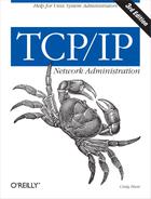
To illustrate these concepts and provide consistent examples, we’ll use an imaginary corporate network. Our imaginary company brings together authors to write computer books and conduct training. Our company network is made up of several networks at our training facilities and publishing office, as well as a connection to the Internet. We are responsible for managing the Ethernet in the computing center. This network’s structure, or topology, is shown in Figure 2-1.
The icons in the figure represent computer systems. There are, of course, several other imaginary systems on our imaginary network, but we’ll use the hosts rodent (a workstation) and crab (a system that serves as a gateway) for most of our examples. The thick line is our computer center Ethernet, and the oval is the local network that connects our various corporate networks. The cloud is the Internet, and the numbers are IP addresses.
An IP address is a 32-bit value that uniquely identifies every device attached to a TCP/IP network. IP addresses are usually written as four decimal numbers separated by dots (periods) in a format called dotted decimal notation .[7] Each decimal number represents an 8-bit byte of the 32-bit address, and each of the four numbers is in the range 0-255 (the decimal values possible in a single byte).
IP addresses are often called host addresses. While this is common usage, it is slightly misleading. IP addresses are assigned to network interfaces, not to computer systems. A gateway, such as crab (see Figure 2-1), has a different address for each network to which it is connected. The gateway is known to other devices by the address associated with the network that it shares with those devices. For example, rodent addresses crab as 172.16.12.1 while external hosts address it as 10.104.0.19.
Systems can be addressed in three different ways. Individual systems are directly addressed by a host address, which is called a unicast address . A unicast packet is addressed to one individual host. Groups of systems can be addressed using a multicast address, e.g., 224.0.0.9. Routers along the path from the source to the destination recognize the special address and route copies of the packet to each member of the multicast group.[8] All systems on a network are addressed using the broadcast address, e.g., 172.16.255.255. The broadcast address depends on the broadcast capabilities of the underlying physical network.
The broadcast address is a good example of the fact that not all network addresses or host addresses can be assigned to a network device. Some host addresses are reserved for special uses. On all networks, host numbers 0 and 255 are reserved. An IP address with all host bits set to 1 is a broadcast address.[9] The broadcast address for network 172.16 is 172.16.255.255. A datagram sent to this address is delivered to every individual host on network 172.16. An IP address with all host bits set to 0 identifies the network itself. For example, 10.0.0.0 refers to network 10, and 172.16.0.0 refers to network 172.16. Addresses in this form are used in routing tables to refer to entire networks.
Network addresses with a first byte value greater than 223 cannot be assigned to a physical network, because those addresses are reserved for special use. There are two other network addresses that are used only for special purposes: network 0.0.0.0 designates the default route and network 127.0.0.1 is the loopback address. The default route is used to simplify the routing information that IP must handle. The loopback address simplifies network applications by allowing the local host to be addressed in the same manner as a remote host. These special network addresses play an important part when configuring a host, but these addresses are not assigned to devices on real networks. Despite these few exceptions, most addresses are assigned to physical devices and are used by IP to deliver data to those devices.
The Internet Protocol moves data between hosts in the form of datagrams. Each datagram is delivered to the address contained in the Destination Address (word 5) of the datagram’s header. The Destination Address is a standard 32-bit IP address, which contains sufficient information to uniquely identify a network and a specific host on that network.
An IP address contains a network part and a host part, but the format of these parts is not the same in every IP address. The number of address bits used to identify the network and the number used to identify the host vary according to the prefix length of the address. The prefix length is determined by the address bit mask.
An address bit mask works like this: if a bit is on in the mask, that equivalent bit in the address is interpreted as a network bit; if a bit in the mask is off, the bit belongs to the host part of the address. For example, if address 172.22.12.4 is given the network mask 255.255.255.0, which has 24 bits on and 8 bits off, the first 24 bits are the network number and the last 8 bits are the host address. Combining the address and the mask tells us that this is the address of host 4 on network 172.22.12.
Specifying both the address and the mask in dotted decimal
notation is cumbersome when writing out addresses. A shorthand
notation is available for writing an address with its associated
address mask. Instead of writing network 172.31.26.32 with a mask of
255.255.255.224, we can write 172.31.26.32/27. The format of this
notation is address/prefix-length, where
prefix-length is the number of bits in the network portion of the
address. Without this notation, the address 172.31.26.32 could easily
be misinterpreted.
Organizations usually obtain official IP addresses by purchasing a block of addresses from their Internet service provider. The ISP normally assigns a single organization a continuous block of addresses that is appropriate for the needs of the organization. For example, a moderately large business might purchase 192.168.16.0/20 while a small business might buy 192.168.32.0/24. Because the prefix shows the length of the network portion of the address, the number of host addresses that are available to an organization (the host portion of the address) is determined by subtracting the prefix from the total number of bits in an address, which is 32. Thus a prefix of 20 leaves 12 bits that are available to be locally assigned. This is called a “12-bit block” of addresses. A prefix of 24 creates an “8-bit block.” Of the two sample address blocks, the first is a 12-bit block that encompasses 4,096 addresses from 192.168.16.0 to 192.168.31.255, and the second is an 8-bit block that includes the 256 addresses from 192.168.32.0 to 192.168.32.255.
Each of these address blocks appears to the outside world to be a single “network” address. Thus external routers have one route to the block 192.168.16.0/20 and one route to the block 192.168.32.0/24, regardless of the size of the address block. Internally, however, the organization may have several separate physical networks within the address block. The flexibility of address masks means that service providers can assign arbitrary length blocks of addresses to their customers, and the customers can subdivide those address blocks using different length masks.
The structure of an IP address can be locally modified by using host address bits as additional network address bits. Essentially, the “dividing line” between network address bits and host address bits is moved, creating additional networks but reducing the maximum number of hosts that can belong to each network. These newly designated network bits define an address block within the larger address block, which is called a subnet.
Organizations usually decide to subnet in order to overcome topological or organizational problems. Subnetting allows decentralized management of host addressing. With the standard addressing scheme, a central administrator is responsible for managing host addresses for the entire network. By subnetting, the administrator can delegate address assignment to smaller organizations within the overall organization—which may be a political expedient, if not a technical requirement. If you don’t want to deal with the data processing department, for example, assign them their own subnet and let them manage it themselves.
Subnetting can also be used to overcome hardware differences and distance limitations. IP routers can link dissimilar physical networks together, but only if each physical network has its own unique network address. Subnetting divides a single address block into many unique subnet addresses, so that each physical network can have its own unique address.
A subnet is defined by changing the bit mask of the IP address. A subnet mask functions in the same way as a normal address mask: an “on” bit is interpreted as a network bit; an “off” bit belongs to the host part of the address. The difference is that a subnet mask is only used locally. On the outside, the address is still interpreted using the address mask known to the outside world.
Assume you have a small real estate business that has been assigned the address block 192.168.32.0/24. The bit mask associated with that address block is 255.255.255.0, and the block contains 256 addresses. Further, assume that your business has 10 offices, each with a half-dozen computers, and that you want to allocate some addresses to each office and keep some for future expansion. You can subdivide the 256 address block with a subnet mask that extends the network portion of the address by a few additional bits.
To subdivide 192.168.32.0/24 into 16 subnets, use the mask 255.255.255.240, i.e., 192.168.32.0/28. The first three bytes contain the original network address block; the fourth byte is divided between the subnet address and the address of the host on that subnet. Applying this mask defines the four high-order bits of the fourth byte as the subnet part of the address, and the remaining four bits—the last four bits of the fourth byte—as the host portion of the address. This creates 16 subnets that each contain 14 host addresses, which is better suited to the network topology of your small real estate business. Table 2-1 shows the subnets and host addresses produced by applying this subnet mask to network address 192.168.32.0/24.
Table 2-1. Effects of a subnet mask
Network number | Host address range | Broadcast address |
|---|---|---|
192.168.32.0 | 192.168.32.1 - 192.168.32.14 | 192.168.32.15 |
192.168.32.16 | 192.168.32.17 - 192.168.32.30 | 192.168.32.31 |
192.168.32.32 | 192.168.32.33 - 192.168.32.46 | 192.168.32.47 |
192.168.32.48 | 192.168.32.49 - 192.168.32.62 | 192.168.32.63 |
192.168.32.64 | 192.168.32.65 - 192.168.32.78 | 192.168.32.79 |
192.168.32.80 | 192.168.32.81 - 192.168.32.94 | 192.168.32.95 |
192.168.32.96 | 192.168.32.97 - 192.168.32.110 | 192.168.32.111 |
192.168.32.112 | 192.168.32.113 - 192.168.32.126 | 192.168.32.127 |
192.168.32.128 | 192.168.32.129 - 192.168.32.142 | 192.168.32.143 |
192.168.32.144 | 192.168.32.145 - 192.168.32.158 | 192.168.32.159 |
192.168.32.160 | 192.168.32.161 - 192.168.32.174 | 192.168.32.175 |
192.168.32.176 | 192.168.32.177 - 192.168.32.190 | 192.168.32.191 |
192.168.32.192 | 192.168.32.193 - 192.168.32.206 | 192.168.32.207 |
192.168.32.208 | 192.168.32.209 - 192.168.32.222 | 192.168.32.223 |
192.168.32.224 | 192.168.32.225 - 192.168.32.238 | 192.168.32.239 |
192.168.32.240 | 192.168.32.241 - 192.168.32.254 | 192.168.32.255 |
In Table 2-1, the first row describes a subnet with a subnet number that is all 0s (the first four bits of the fourth byte are all set to 0). The last row in the table describes a subnet with a subnet number that is all 1s (the first four bits of the fourth byte are all set to 1). Originally, the RFCs implied that you should not use subnet numbers of all 0s or all 1s. However, RFC 1812, Requirements for IP Version 4 Routers, makes it clear that subnets of all 0s and all 1s are legal and should be supported by all routers. Some older routers did not allow the use of these addresses despite the newer RFCs. Today’s router software and hardware should make it possible for you to reliably use all subnet addresses.
You don’t have to manually calculate a table like this to know what subnets and host addresses are produced by a subnet mask. The calculations have already been done for you. RFC 1878, Variable Length Subnet Table For IPv4, lists all possible subnet masks and the valid addresses they produce.
RFC 1878 describes all 32 prefix values. But little documentation is needed because the prefix is easy to understand and remember. Writing 10.104.0.19 as 10.104.0.19/8 shows that this address has 8 bits for the network number and therefore 24 bits for the host number. Unfortunately, things are not always this neat. Sometimes the address is not given an explicit address mask, and you need to know how to determine the natural mask that an address will be assigned by default.
Originally, the IP address space was divided into a few fixed-length structures called address classes. The three main address classes were class A, class B, and class C. IP software determined the class, and therefore the structure, of an address by examining its first few bits. Address classes are no longer used, but the same rules that were used to determine the address class are now used to create the default address mask, which is called the natural mask . These rules are as follows:
If the first bit of an IP address is 0, the default mask is 8 bits long (prefix 8). This is the same as the old class A network address format. The first 8 bits identify the network, and the last 24 bits identify the host.
If the first 2 bits of the address are 1 0, the default mask is 16 bits long (prefix 16), which is the same as the old class B network address format. The first 16 bits identify the network, and the last 16 bits identify the host.
If the first 3 bits of the address are 1 1 0, the default mask is 24 bits long (prefix 24). This mask is the same as the old class C network address format. The first 24 bits are the network address, and the last 8 bits identify the host.
If the first 4 bits of the address are 1 1 1 0, it is a multicast address. These addresses were sometimes called class D addresses, but they don’t really refer to specific networks. Multicast addresses are used to address groups of computers all at one time. They identify a group of computers that share a common application, such as a videoconference, as opposed to a group of computers that share a common network. All bits in a multicast address are significant for routing, so the default mask is 32 bits long (prefix 32).
When an IP address is written in dotted decimal format, it is sometimes easier to think of the address as four 8-bit bytes instead of as a 32-bit value. We can look at the address as composed of full bytes of network address and full bytes of host address when using the natural mask, because the three default masks all create prefix lengths that are multiples of 8. A simple way to determine the default mask is to look at the first byte of the address. If the value of the first byte is:
Less than 128, the default address mask is 8 bits long; the first byte is the network number, and the next three bytes are the host address.
From 128 to 191, the default address mask is 16 bits long; the first two bytes identify the network, and the last two bytes identify the host.
From 192 to 223, the default address mask is 24 bits long; the first three bytes are the network address, and the last byte is the host number.
From 224 to 239, the address is multicast. The entire address identifies a specific multicast group; therefore the default mask is 32 bits.
Greater than 239, the address is reserved. We can ignore reserved addresses.
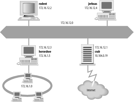
Figure 2-2 illustrates the two techniques for determining the default address structure. The first address is 10.104.0.19. The first bit of this address is 0; therefore, the first 8 bits define the network and the last 24 bits define the host. Explained in a byte-oriented manner, the first byte is less than 128, so the address is interpreted as host 104.0.19 on network 10. One byte specifies the network and three bytes specify the host.
The second address is 172.16.12.1. The two high-order bits are 1 0, meaning that 16 bits define the network and 16 bits define the host. Viewed in a byte-oriented way, the first byte falls between 128 and 191, so the address refers to host 12.1 on network 172.16. Two bytes identify the network and two identify the host.
Finally, in the address 192.168.16.1, the three high-order bits are 1 1 0, indicating that 24 bits represent the network and 8 bits represent the host. The first byte of this address is in the range from 192 to 223, so this is the address of host 1 on network 192.168.16—three network bytes and one host byte.
Evaluating addresses according to the class rules discussed above limits the length of network numbers to 8, 16, or 24 bits—1, 2, or 3 bytes. The IP address, however, is not really byte-oriented. It is 32 contiguous bits. The address bit mask provides a flexible way to define the network and host portions of an address. IP uses the network portion of the address to route the datagram between networks. The full address, including the host information, is used to identify an individual host. Because of the dual role of IP addresses, the flexibility of address masks not only makes more addresses available for use, but also has a positive impact on routing.
The IP address, which provides universal addressing across all of the networks of the Internet, is one of the great strengths of the TCP/IP protocol suite. However, the original class structure of the IP address had weaknesses. The TCP/IP designers did not envision the enormous scale of today’s network. When TCP/IP was being designed, networking was limited to large organizations that could afford substantial computer systems. The idea of a powerful Unix system on every desktop did not exist. At that time, a 32-bit address seemed so large that it was divided into classes to reduce the processing load on routers, even though dividing the address into classes sharply reduced the number of host addresses actually available for use. For example, assigning a large network a single class B address instead of six class C addresses reduced the load on the router because the router needed to keep only one route for that entire organization. However, an organization that was assigned the class B address probably did not have 64,000 computers, so most of the host addresses available to the organization were never used.
The class-structured address design was critically strained by the rapid growth of the Internet. At one point it appeared that all class B addresses might be rapidly exhausted. The rapid depletion of the class B addresses showed that three primary address classes were not enough: class A was much too large and class C was much too small. Even a class B address was too large for many networks, but was used because it was better than the alternatives.
The obvious solution to the class B address crisis was to force organizations to use multiple class C addresses. There were millions of these addresses available and they were in no immediate danger of depletion. As is often the case, the obvious solution was not as simple as it seemed. Each class C address requires its own entry within the routing table. Assigning thousands or millions of class C addresses would cause the routing table to grow so rapidly that the routers would soon be overwhelmed. The solution required the new way of looking at addresses that address masks provide; it also required a new way of assigning addresses.
Originally network addresses were assigned in more or less sequential order as they were requested. This worked fine when the network was small and centralized. However, it did not take network topology into account. Thus, only random chance determined if the same intermediate routers would be used to reach network 195.4.12.0 and network 195.4.13.0, which makes it difficult to reduce the size of the routing table. Addresses can be aggregated only if they are contiguous numbers and are reachable through the same route. For example, if addresses are contiguous for one service provider, a single route can be created for that aggregation because that service provider will have a limited number of connections to the Internet. But if one network address is in France and the next contiguous address is in Australia, creating a consolidated route for these addresses is not possible.
Today, large, contiguous blocks of addresses are assigned to large network service providers in a manner that better reflects the topology of the network. The service providers then allocate chunks of these address blocks to the organizations to which they provide network services. Because the assignment of addresses reflects the topology of the network, it permits route aggregation. Under this scheme, we know that network 195.4.12.0 and network 195.4.13.0 are reachable through the same intermediate routers. In fact, both of these addresses are in the range of the addresses assigned to Europe, 194.0.0.0 to 195.255.255.255.
Assigning addresses that reflect the topology of the network enables route aggregation but does not implement it. As long as network 195.4.12.0 and network 195.4.13.0 were interpreted as separate class C addresses, they still required separate entries in the routing table. The development of address masks not only increased the usable address space, but it improved routing.
The use of an address mask instead of the old address classes to determine the destination network is called Classless Inter-Domain Routing (CIDR).[10] CIDR requires modifications to the routers and routing protocols. The protocols need to distribute, along with the destination addresses, address masks that define how the addresses are interpreted. The routers and hosts need to know how to interpret these addresses as “classless” addresses and how to apply the bit mask that accompanies the address. All new operating systems and routing protocols support address masks.
CIDR was intended as an interim solution, but it has proved much more durable than its designers imagined. CIDR has provided address and routing relief for many years and is capable of providing it for many more years to come. The long-term solution for address depletion is to replace the current addressing scheme with a new one. In the TCP/IP protocol suite, addressing is defined by the IP protocol. Therefore, to define a new address structure, the Internet Engineering Task Force (IETF) created a new version of IP called IPv6.
IPv6 is an improvement on the IP protocol based on 20 years of operational experience. The original motivation for the new protocol was the threat of address depletion. IPv6 has a very large 128-bit address, so address depletion is not an issue. The large address also makes it possible to use a hierarchical address structure to reduce the burden on routers while still maintaining more than enough addresses for future network growth. But large addresses are only one of the benefits of the new protocol. Other benefits of IPv6 are:
Improved security built into the protocol
Simplified, fixed-length, word-aligned headers to speed header processing and reduce overhead
Improved techniques for handling header options
IPv6 has several good features, but it is still not widely used. This is partly because enhancements to IPv4, improvements in hardware performance, and changes in the way that networks are configured have reduced the demand for the new features of IPv6.
A critical shortage of addresses did not materialize for three reasons:
CIDR makes the assignment of addresses more flexible, which in turn makes more addresses available and permits aggregation to reduce the burden on routers.
Private addresses and NAT have greatly reduced the demand for official addresses. Many organizations prefer to use private addresses for all systems on their internal networks because private addresses reduce the administrative burden and improve security.
Permanent, fixed address assignment is less common than dynamic address assignment. The majority of systems use dynamic addresses temporarily assigned by the configuration protocol DHCP.
The creation of the IPsec standards for IPv4 lessened the need for the security enhancements of IPv6. In fact, many of the security tools and features available for IPv4 systems are not being fully utilized, indicating that the demand for tools that secure the link may have been overestimated.
IPv6 eliminates hop-by-hop segmentation, has a more efficient header design, and features enhanced option processing. These things make it more efficient to process IPv6 packets than to handle IPv4 packets. However, for the vast majority of systems, this increased efficiency is not needed because processing IP datagrams is a very minor task. Most systems are at the edge of the network and handle relatively few communications packets. Processor speed and memory have increased enormously while hardware prices have fallen. Most managers would rather buy more hardware using the proven IPv4 protocol than risk implementing the new IPv6 protocol just to save a few machine cycles. Only those systems located near the core of the network would truly benefit from this efficiency, and although important, those systems are relatively few in number.
All of these things have worked together to lessen the demand for IPv6. This lack of demand has limited the number of organizations that have adopted IPv6 as their primary communications protocol, and a large user community is the one thing that a protocol needs to be truly successful. We use communications protocols to communicate with other people. If there are not enough people using the protocol, we don’t feel the need to use it. IPv6 is still in the early-adopter phase. Most organizations do not use IPv6 at all, and many that do use it only for experimental purposes.[11] Between organizations, most IPv6 communications are encapsulated inside IPv4 datagrams and sent over the Internet inside IPv4 tunnels. It will be some time before it is the primary protocol of operational networks.
If you run an operational network, you should not be overly concerned with IPv6. The current generation of TCP/IP (IPv4), with the enhancements that CIDR and other extensions provide, should be more than adequate for your current network needs. On your network and the Internet, you will use IPv4 and 32-bit IP addresses.
Chapter 1 described the evolution of the Internet architecture over the years. Along with these architectural changes have come changes in the way that routing information is disseminated within the network.
In the original Internet structure, there was a hierarchy of gateways. This hierarchy reflected the fact that the Internet was built upon the existing ARPAnet. When the Internet was created, the ARPAnet was the backbone of the network: a central delivery medium to carry long-distance traffic. This central system was called the core, and the centrally managed gateways that interconnected it were called the core gateways.
In that hierarchical structure, routing information about all of the networks on the Internet was passed into the core gateways. The core gateways processed the information and then exchanged it among themselves using the Gateway to Gateway Protocol (GGP). The processed routing information was then passed back out to the external gateways. The core gateways maintained accurate routing information for the entire Internet.
Using the hierarchical core router model to distribute routing information has a major weakness: every route must be processed by the core. This places a tremendous processing burden on the core, and as the Internet grew larger the burden increased. In network-speak, we say that this routing model does not “scale well.” For this reason, a new model emerged.
Even in the days of a single Internet core, groups of independent networks called autonomous systems existed outside of the core. The term autonomous system (AS) has a formal meaning in TCP/IP routing. An autonomous system is not merely an independent network. It is a collection of networks and gateways with its own internal mechanism for collecting routing information and passing it to other independent network systems. The routing information passed to the other network systems is called reachability information. Reachability information simply says which networks can be reached through that autonomous system. In the days of a single Internet core, autonomous systems passed reachability information into the core for processing. The Exterior Gateway Protocol (EGP) was the protocol used to pass reachability information between autonomous systems and into the core.
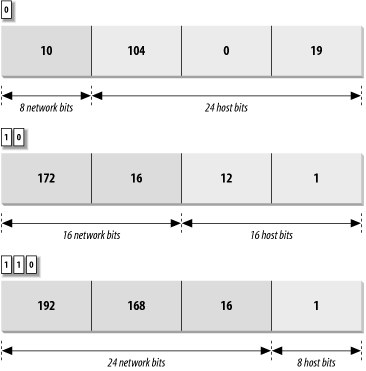
The new routing model is based on co-equal collections of autonomous systems called routing domains. Routing domains exchange routing information with other domains using Border Gateway Protocol (BGP). Each routing domain processes the information it receives from other domains. Unlike the hierarchical model, this model does not depend on a single core system to choose the “best” routes. Each routing domain does this processing for itself; therefore, this model is more expandable. Figure 2-3 represents this model with three intersecting circles. Each circle is a routing domain. The overlapping areas are border areas, where routing information is shared. The domains share information but do not rely on any one system to provide all routing information.
The problem with this model is: how are “best” routes determined in a global network if there is no central routing authority, like the core, that is trusted to determine the “best” routes? In the days of the NSFNET, the policy routing database (PRDB) was used to determine whether the reachability information advertised by an autonomous system was valid. But now, even the NSFNET does not play a central role.
To fill this void, NSF created the Routing Arbiter (RA) servers when it created the Network Access Points (NAPs) that provide interconnection points for the various service provider networks. A route arbiter is located at each NAP. The server provides access to the Routing Arbiter Database (RADB), which replaced the PRDB. ISPs can query servers to validate the reachability information advertised by an autonomous system.
The RADB is only part of the Internet Routing Registry (IRR). As befits a distributed routing architecture, there are multiple organizations that validate and register routing information. Europeans were the pioneers in this. The Reseaux IP Europeens (RIPE) Network Control Center (NCC) provides the routing registry for European IP networks. Big network carriers provide registries for their customers. All of the registries share a common format based on the RIPE-181 standard.
Many ISPs do not use the route servers. Instead they depend on formal and informal bilateral agreements, where two ISPs get together and decide what reachability information each will accept from the other. They create, in effect, private routing policies. Small ISPs have criticized the routing policies of the tier-one providers, claiming that they limit competition. In response, most tier-one providers have promised to make the policies public, which should clarify the basis for the current architecture and may even spark more changes.
Creating an effective routing architecture continues to be a major challenge for the Internet, and the routing architecture will certainly evolve over time. No matter how it is derived, the routing information eventually winds up in your local gateway, where it is used by IP to make routing decisions.
Gateways route data between networks, but all network devices, hosts as well as gateways, must make routing decisions. For most hosts, the routing decisions are simple:
IP routing decisions are simply table lookups. Packets are routed toward their destinations as directed by the routing table (also called the forwarding table). The routing table maps destinations to the router and network interface that IP must use to reach that destination. Examining the routing table on a Linux system shows this.
On a Linux system, use the route
command with the -n option to display
the routing table.[12] The -n option prevents
route from converting IP addresses to
hostnames, which gives a clearer display. Here is a routing table from a
sample Red Hat system:
            # route -n
Kernel IP routing table
Destination   Gateway      Genmask        Flags Metric Ref   Use Iface
172.16.55.0   0.0.0.0      255.255.255.0  U     0      0       0 eth0
172.16.50.0   172.16.55.36 255.255.255.0  UG    0      0       0 eth0
127.0.0.0     0.0.0.0      255.0.0.0      U     0      0       0 lo
0.0.0.0       172.16.55.1  0.0.0.0        UG    0      0       0 eth0
On a Linux system, the route
-n command displays the routing table
with the following fields:
DestinationThe value against which the destination IP address is matched.
GatewayGenmaskThe address mask used to match an IP address to the value shown in the Destination field.
FlagsCertain characteristics of this route. The possible Linux flag values are:[13]
UHIndicates that this is a route to a specific host (most routes are to networks).
GIndicates that the route uses an external gateway. The system’s network interfaces provide routes to directly connected networks. All other routes use external gateways. Directly connected networks do not have the G flag set; all other routes do.
RIndicates a route that was installed, probably by a dynamic routing protocol running on this system, using the
reinstateoption.DIndicates that this route was added because of an ICMP Redirect Message. When a system learns of a route via an ICMP Redirect, it adds the route to its routing table so that additional packets bound for that destination will not need to be redirected. The system uses the D flag to mark these routes.
MIndicates a route that was modified, probably by a dynamic routing protocol running on this system, using the
modoption.AIndicates a cached route that has an associated entry in the ARP table.
CIndicates that this route came from the kernel routing cache. Most systems use two routing tables: the Forwarding Information Base (FIB), which is the table we are interested in because it is used for the routing decision, and the kernel routing cache, which lists the source and destination of recently used routes. This flag is documented, but I have never seen the C flag in a routing table listing, even when listing the routing cache.
LIndicates that the destination of this route is one of the addresses of this computer. These “local routes” are found only in the routing cache.
BIndicates a route whose destination is a broadcast address. These “broadcast routes” are found only in the routing cache. Solaris assigns the flag to both broadcast addresses and network addresses; i.e., both 172.16.255.255 and 172.16.0.0 are given the B flag by Solaris systems that live on network 172.16.0.0/16.
IIndicates a route that uses the loopback interface for some purpose other than addressing the loopback network. These “internal routes” are found only in the routing cache.
!Indicates that datagrams bound for this destination will be rejected. Linux permits you to manually install “negative” routes. These are routes that explicitly block data bound for a specific destination. This is Linux-specific and rarely used, but it is a possible flag setting.
- Metric
The “cost” of the route. The metric is used to sort duplicate routes if any appear in the table. Beyond this, a dynamic routing protocol is required to make use of the metric.
- Ref
The number of times the route has been referenced to establish a connection. This value is not used by Linux systems.
- Use
- Iface
The name of the network interface[14] used by this route.
Each entry in the routing table starts with a destination value. The destination value is the key against which the IP address is matched to determine if this is the correct route to use to reach the IP address. The destination value is usually called the “destination network,” although it does not need to be a network address. The destination value can be a host address, a multicast address, an address block that covers an aggregation of many networks, or a special value for the default route or loopback address. In all cases, however, the Destination field contains the value against which the destination address from the IP packet is matched to determine if IP should deliver the datagram using this route.
The Genmask field is the bit mask that IP applies to the destination address from the packet to see if the address matches the destination value in the table. If a bit is on in the bit mask, the corresponding bit in the destination address is significant for matching the address. Thus, the address 172.16.50.183 would match the second entry in the sample table because ANDing the address with 255.255.255.0 yields 172.16.50.0.
When an address matches an entry in the table, the Gateway
field tells IP how to reach the specified destination. If
the Gateway field contains the IP address of a router, the router is
used. If the Gateway field contains all 0s (0.0.0.0 when route is run with -n) or an asterisk (* when route is run without -n), the destination network is a directly
connected network and the “gateway” is the computer’s network interface.
The last field displayed for each table entry is the network interface
used for the route. In the example, it is either the first Ethernet
interface (eth0) or the loopback interface
(lo). The destination, gateway, mask, and interface
define the route.
The remaining four fields (Ref, Use, Flags, and Metric) display supporting information about the route. These informational fields are of only marginal value. Some systems keep an accurate count in the Ref field; others, such as Linux, don’t really use it. Linux uses the Use field to count the number of times a route needed to be looked up because it was not in the routing cache when IP needed it. Some other systems show the number of packets transmitted via the route in the Use field. The Flags field displays information that is often obvious even without the flags: every route has the U flag set because every route in the routing table is up by definition, and looking at the Gateway field tells you whether or not an external gateway is used without looking for the G flag. The Metric value is used only if you run some version of the Routing Information Protocol (RIP) on your system. Don’t be distracted by this information. The heart of the routing table is the route, which is composed of the destination, the mask, the gateway, and the interface.
IP uses the information from the routing table (the forwarding
table) to construct the routes used for active connections. The routes
associated with active connections are stored in the routing cache. On Linux systems, the routing cache can be examined by adding the
-C argument to the route command line:
            $ route -Cn
Kernel IP routing cache
Source          Destination     Gateway        Flags Metric Ref Use Iface
127.0.0.1       127.0.0.1       127.0.0.1      l     0      0     0 lo
192.203.230.10  172.16.55.3     172.16.55.3    l     0      0     0 lo
172.16.55.1     172.16.55.255   172.16.55.255  ibl   0      0   243 lo
172.16.55.2     172.16.55.255   172.16.55.255  ibl   0      0    15 lo
172.16.55.3     192.203.230.10  172.16.55.1          0      0     0 eth0
127.0.0.1       127.0.0.1       127.0.0.1      l     0      0     0 lo
172.16.55.3     132.163.4.9     172.16.55.1          0      0     0 eth0
172.16.55.2     172.16.55.3     172.16.55.3    il    0      0   149 lo
172.16.55.3     172.16.55.2     172.16.55.2          0      1     0 eth0
132.163.4.9     172.16.55.3     172.16.55.3    l     0      0     0 lo
The routing cache is different from the routing table because the cache shows established routes. The routing table is used to make routing decisions; the routing cache is used after the decision is made. The routing cache shows the source and destination of a network connection and the gateway and interface used to make that connection.
Linux provides a good example for showing the contents of the
routing table because the Linux route
command displays the table so clearly. On Solaris systems, the route command has a very different syntax.
When running Solaris, display the routing table’s contents with the
netstat -nr command. The -r option tells
netstat to display the routing table,
and the -n option tells netstat to display the table in numeric
form.[15]
            % netstat -nr
Routing Table: IPv4
Destination     Gateway        Flags  Ref    Use   Interface
-----------    -----------     -----  ----  -----  ---------
127.0.0.1      127.0.0.1       UH      1      298      lo0
default        172.16.12.1     UG      2    50360
172.16.12.0    172.16.12.2     U      40   111379      dnet0
172.16.2.0     172.16.12.3     UG      4     1179
172.16.1.0     172.16.12.3     UG     10     1113
172.16.3.0     172.16.12.3     UG      2     1379
172.16.4.0     172.16.12.3     UG      4     1119
The first table entry is the loopback route
for the local host. This is the loopback address mentioned
earlier as a reserved network number. Because every system uses the
loopback route to send datagrams to itself, an entry for the loopback
interface is in every host’s routing table. The H flag is set because
Solaris creates a route to a specific host (127.0.0.1), not a route to
an entire network (127.0.0.0). We’ll see the loopback facility again
when we discuss kernel configuration and the ifconfig command. For now, however, our real
interest is in external routes.
Another unique entry in this routing table is the one with the word “default” in the destination field. This entry is for the default route, and the gateway specified in this entry is the default gateway. The default route is the other reserved network number mentioned earlier: 0.0.0.0. The default gateway is used whenever there is no specific route in the table for a destination network address. For example, this routing table has no entry for network 192.168.16.0. If IP receives any datagrams addressed to this network, it will send them via the default gateway 172.16.12.1.
All of the gateways that appear in the routing table are on networks directly connected to the local system. In the sample shown above, this means that the gateway addresses all begin with 172.16.12 regardless of the destination address. This is the only network to which this sample host is directly attached, and therefore it is the only network to which it can directly deliver data. The gateways that a host uses to reach the rest of the Internet must be on its subnet.
In Figure 2-4, the IP layer of two hosts and a gateway on our imaginary network is replaced by a small piece of a routing table, showing destination networks and the gateways used to reach those destinations. Assume that the address mask used for network 172.16.0.0 is 255.255.255.0. When the source host (172.16.12.2) sends data to the destination host (172.16.1.2), it applies the address mask to determine that it should look for the destination network address 172.16.1.0 in the routing table. The routing table in the source host shows that data bound for 172.16.1.0 is sent to gateway 172.16.12.3. The source host forwards the packet to the gateway. The gateway does the same steps and looks up the destination address in its routing table. Gateway 172.16.12.3 then makes direct delivery through its 172.16.1.5 interface. Examining the routing tables in Figure 2-4 shows that all systems list only gateways on networks to which they are directly connected. This is illustrated by the fact that 172.16.12.1 is the default gateway for both 172.16.12.2 and 172.16.12.3, but because 172.16.1.2 cannot reach network 172.16.12.0 directly, it has a different default route.
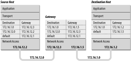
A routing table does not contain end-to-end routes. A route points only to the next gateway, called the next hop, along the path to the destination network.[16] The host relies on the local gateway to deliver the data, and the gateway relies on other gateways. As a datagram moves from one gateway to another, it should eventually reach one that is directly connected to its destination network. It is this last gateway that finally delivers the data to the destination host.
IP uses the network portion of the address to route the datagram between networks. The full address, including the host information, is used to make final delivery when the datagram reaches the destination network.
The IP address and the routing table direct a datagram to a specific physical network, but when data travels across a network, it must obey the physical layer protocols used by that network. The physical networks underlying the TCP/IP network do not understand IP addressing. Physical networks have their own addressing schemes, and there are as many different addressing schemes as there are different types of physical networks. One task of the network access protocols is to map IP addresses to physical network addresses.
The most common example of this Network Access Layer function is the translation of IP addresses to Ethernet addresses. The protocol that performs this function is Address Resolution Protocol (ARP), which is defined in RFC 826.
The ARP software maintains a table of translations between IP addresses and Ethernet addresses. This table is built dynamically. When ARP receives a request to translate an IP address, it checks for the address in its table. If the address is found, it returns the Ethernet address to the requesting software. If the address is not found, ARP broadcasts a packet to every host on the Ethernet. The packet contains the IP address for which an Ethernet address is sought. If a receiving host identifies the IP address as its own, it responds by sending its Ethernet address back to the requesting host. The response is then cached in the ARP table.
The arp command displays the contents of the ARP table. To
display the entire ARP table, use the arp -a command. Individual entries can be displayed by specifying
a hostname on the arp command line.
For example, to check the entry for rodent in the
ARP table on crab, enter:
            % arp rodent
rodent (172.16.12.2) at 0:50:ba:3f:c2:5e
Checking all entries in the table with the -a option produces the following
output:
            % arp -a

Net to Media Table: IPv4
Device   IP Address               Mask      Flags   Phys Addr
------ -------------------- --------------- ----- ---------------
dnet0  rodent               255.255.255.255       00:50:ba:3f:c2:5e
dnet0  crab                 255.255.255.255 SP    00:00:c0:dd:d4:da
dnet0  224.0.0.0            240.0.0.0       SM    01:00:5e:00:00:00
This table tells you that when crab forwards datagrams addressed to rodent, it puts those datagrams into Ethernet frames and sends them to Ethernet address 00:50:ba:3f:c2:5e.
One of the entries in the sample table (rodent) was added dynamically as a result of queries by crab. Two of the entries (crab and 224.0.0.0) are static entries added as a result of the configuration of crab. We know this because both these entries have an S, for “static,” in the Flags field. The special 224.0.0.0 entry is for all multicast addresses. The M flag means “mapping” and is used only for the multicast entry. On a broadcast medium like Ethernet, the Ethernet broadcast address is used to make final delivery to a multicast group.
The P flag on the crab entry means that this entry will be “published.” The “publish” flag indicates that when an ARP query is received for the IP address of crab, this system answers it with the Ethernet address 00:00:c0:dd:d4:da. This is logical because this is the ARP table on crab. However, it is also possible to publish Ethernet addresses for other hosts, not just for the local host. Answering ARP queries for other computers is called proxy ARP.
For example, assume that 24seven is the server for a remote system named clock connected via a dial-up telephone line. Instead of setting up routing to the remote system, the administrator of 24seven could place a static, published entry in the ARP table with the IP address of clock and the Ethernet address of 24seven. Now when 24seven hears an ARP query for the IP address of clock, it answers with its own Ethernet address. The other systems on the network therefore send packets destined for clock to 24seven. 24seven then forwards the packets on to clock over the telephone line. Proxy ARP is used to answer queries for systems that can’t answer for themselves.
ARP tables normally don’t require any attention because they are built automatically by the ARP protocol, which is very stable. However, if things go wrong, the ARP table can be manually adjusted. See Section 13.4.2 in Chapter 13 .
Once data is routed through the network and delivered to a specific host, it must be delivered to the correct user or process. As the data moves up or down the TCP/IP layers, a mechanism is needed to deliver it to the correct protocols in each layer. The system must be able to combine data from many applications into a few transport protocols, and from the transport protocols into the Internet Protocol. Combining many sources of data into a single data stream is called multiplexing.
Data arriving from the network must be demultiplexed: divided for delivery to multiple processes. To accomplish this task, IP uses protocol numbers to identify transport protocols, and the transport protocols use port numbers to identify applications.
Some protocol and port numbers are reserved to identify well-known services . Well-known services are standard network protocols, such as FTP and Telnet, that are commonly used throughout the network. The protocol numbers and port numbers are assigned to well-known services by the Internet Assigned Numbers Authority (IANA). Officially assigned numbers are documented at http://www.iana.org . Unix systems define protocol and port numbers in two simple text files.
The protocol number is a single byte in the third word of the datagram header. The value identifies the protocol in the layer above IP to which the data should be passed.
On a Unix system, the protocol numbers are defined in
/etc/protocols. This file is a simple table
containing the protocol name and the protocol number associated with
that name. The format of the table is a single entry per line,
consisting of the official protocol name, separated by whitespace from
the protocol number. The protocol number is separated by whitespace
from the “alias” for the protocol name. Comments in the table begin
with #. An
/etc/protocols file is shown below:
% cat /etc/protocols
#ident  "@(#)protocols  1.5     99/03/21 SMI"   /* SVr4.0 1.1   */

#
# Internet (IP) protocols
#
ip            0     IP            # pseudo internet protocol number
icmp          1     ICMP          # internet control message protocol
ggp           3     GGP           # gateway-gateway protocol
tcp           6     TCP           # transmission control protocol
egp           8     EGP           # exterior gateway protocol
pup           12    PUP           # PARC universal packet protocol
udp           17    UDP           # user datagram protocol
hmp           20    HMP           # host monitoring protocol
xns-idp       22    XNS-IDP       # Xerox NS IDP
rdp           27    RDP           # "reliable datagram" protocol

#
# Internet (IPv6) extension headers
#
hopopt        0     HOPOPT        # Hop-by-hop options for IPv6
ipv6          41    IPv6          # IPv6 in IP encapsulation
ipv6-route    43    IPv6-Route    # Routing header for IPv6
ipv6-frag     44    IPv6-Frag     # Fragment header for IPv6
esp           50    ESP           # Encap Security Payload for IPv6
ah            51    AH            # Authentication Header for IPv6
ipv6-icmp     58    IPv6-ICMP     # IPv6 internet control message protocol
ipv6-nonxt    59    IPv6-NoNxt    # IPv6No next header extension header
ipv6-opts     60    IPv6-Opts     # Destination Options for IPv6
The listing above is the contents of the /etc/protocols file from a Solaris 8 workstation. This list of numbers is by no means complete. If you refer to the Protocol Numbers section of the IANA web site, you’ll see many more protocol numbers. However, a system needs to include only the numbers of the protocols that it actually uses. Even the list shown above is more than this specific workstation needed; for example, the second half of this table is used only on systems that run IPv6. Don’t worry if your system doesn’t use IPv6 or many of these other protocols. The additional entries do no harm.
What exactly does this table mean? When a datagram arrives and its destination address matches the local IP address, the IP layer knows that the datagram has to be delivered to one of the transport protocols above it. To decide which protocol should receive the datagram, IP looks at the datagram’s protocol number. Using this table, you can see that if the datagram’s protocol number is 6, IP delivers the datagram to TCP; if the protocol number is 17, IP delivers the datagram to UDP. TCP and UDP are the two transport layer services we are concerned with, but all of the protocols listed in the first half of the table use IP datagram delivery service directly. Some, such as ICMP, EGP, and GGP, have already been mentioned. Others haven’t, but you don’t need to be concerned with the minor protocols in order to configure and manage a TCP/IP network.
After IP passes incoming data to the transport protocol, the transport protocol passes the data to the correct application process. Application processes (also called network services) are identified by port numbers, which are 16-bit values. The source port number, which identifies the process that sent the data, and the destination port number, which identifies the process that will receive the data, are contained in the first header word of each TCP segment and UDP packet.
Port numbers below 1024 are reserved for well-known services (like FTP and Telnet) and are assigned by the IANA. Well-known port numbers are considered “privileged ports” that should not be bound to a user process. Ports numbered from 1024 to 49151 are “registered ports.” IANA tries to maintain a registry of services that use these ports, but it does not officially assign port numbers in this range. The port numbers from 49152 to 65535 are the “private ports.” Private port numbers are available for any use.
Port numbers are not unique between transport layer protocols; the numbers are unique only within a specific transport protocol. In other words, TCP and UDP can and do assign the same port numbers. It is the combination of protocol and port numbers that uniquely identifies the specific process to which the data should be delivered.
On Unix systems, port numbers are defined in the /etc/services file. There are many more network applications than there are transport layer protocols, as the size of the /etc/services table shows. A partial /etc/services file from a Solaris 8 workstation is shown here:
               rodent% head -22 /etc/services
#ident  "@(#)services   1.25    99/11/06 SMI"   /* SVr4.0 1.8   */
#
#
# Copyright (c) 1999 by Sun Microsystems, Inc.
# All rights reserved.
#
# Network services, Internet style
#
tcpmux          1/tcp
echo            7/tcp
echo            7/udp
discard         9/tcp           sink null
discard         9/udp           sink null
systat          11/tcp          users
daytime         13/tcp
daytime         13/udp
netstat         15/tcp
chargen         19/tcp          ttytst source
chargen         19/udp          ttytst source
ftp-data        20/tcp
ftp             21/tcp
telnet          23/tcp
The format of this file is very similar to the /etc/protocols file. Each single-line entry starts with the official name of the service separated by whitespace from the port number/protocol pairing associated with that service. The port numbers are paired with transport protocol names because different transport protocols may use the same port number. An optional list of aliases for the official service name may be provided after the port number/protocol pair.
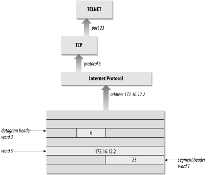
The /etc/services file, combined with the /etc/protocols file, provides all of the information necessary to deliver data to the correct application. A datagram arrives at its destination based on the destination address in the fifth word of the datagram header. Using the protocol number in the third word of the datagram header, IP delivers the data from the datagram to the proper transport layer protocol. The first word of the data delivered to the transport protocol contains the destination port number that tells the transport protocol to pass the data up to a specific application. Figure 2-5 shows this delivery process.
Despite its size, the /etc/services file
does not contain the port number of every important network service.
You won’t find the port number of every Remote Procedure Call (RPC) service in the services file. Sun developed a
different technique for reserving ports for RPC services that doesn’t
involve getting a well-known port number assignment from IANA. RPC
services generally use registered port numbers, which do not need to
be officially assigned. When an RPC service starts, it registers its
port number with the portmapper.
The portmapper is a
program that keeps track of the port numbers being used by RPC
services. When a client wants to use an RPC service, it queries the
portmapper running on the server to
discover the port assigned to the service. The client can find
portmapper because it is assigned
well-known port 111. portmapper
makes it possible to install widely used services without formally
obtaining a well-known port.
Well-known ports are standardized port numbers that enable remote computers to know which port to connect to for a particular network service. This simplifies the connection process because both the sender and receiver know in advance that data bound for a specific process will use a specific port. For example, all systems that offer Telnet do so on port 23.
Equally important is a second type of port number called a dynamically allocated port. As the name implies, dynamically allocated ports are not pre-assigned; they are assigned to processes when needed. The system ensures that it does not assign the same port number to two processes, and that the numbers assigned are above the range of well-known port numbers, i.e., above 1024.
Dynamically allocated ports provide the flexibility needed to support multiple users. If a telnet user is assigned port number 23 for both the source and destination ports, what port numbers are assigned to the second concurrent telnet user? To uniquely identify every connection, the source port is assigned a dynamically allocated port number, and the well-known port number is used for the destination port.
In the telnet example, the first user is given a random source port number and a destination port number of 23 (telnet). The second user is given a different random source port number and the same destination port. It is the pair of port numbers, source and destination, that uniquely identifies each network connection. The destination host knows the source port because it is provided in both the TCP segment header and the UDP packet header. Both hosts know the destination port because it is a well-known port.
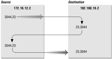
Figure 2-6 shows the exchange of port numbers during the TCP handshake. The source host randomly generates a source port, in this example 3044. It sends out a segment with a source port of 3044 and a destination port of 23. The destination host receives the segment and responds back using 23 as its source port and 3044 as its destination port.
The combination of an IP address and a port number is called a socket. A socket uniquely identifies a single network process within the entire Internet. Sometimes the terms “socket” and “port number” are used interchangeably. In fact, well-known services are frequently referred to as “well-known sockets.” In the context of this discussion, a “socket” is the combination of an IP address and a port number. A pair of sockets, one socket for the receiving host and one for the sending host, define the connection for connection-oriented protocols such as TCP.
Let’s build on the example of dynamically assigned ports and well-known ports. Assume a user on host 172.16.12.2 uses Telnet to connect to host 192.168.16.2. Host 172.16.12.2 is the source host. The user is dynamically assigned a unique port number, 3382. The connection is made to the telnet service on the remote host, which is, according to the standard, assigned well-known port 23. The socket for the source side of the connection is 172.16.12.2.3382 (IP address 172.16.12.2 plus port number 3382). For the destination side of the connection, the socket is 192.168.16.2.23 (address 192.168.16.2 plus port 23). The port of the destination socket is known by both systems because it is a well-known port. The port of the source socket is known by both systems because the source host informed the destination host of the source socket when the connection request was made. The socket pair is therefore known by both the source and destination computers. The combination of the two sockets uniquely identifies this connection; no other connection in the Internet has this socket pair.
This chapter has shown how data moves through the global Internet from one specific process on the source computer to a single cooperating process on the other side of the world. TCP/IP uses globally unique addresses to identify any computer on the Internet. It uses protocol numbers and port numbers to uniquely identify a single process running on that computer.
Routing directs the datagrams destined for a remote process through the maze of the global network. Routing uses part of the IP address to identify the destination network. Every system maintains a routing table that describes how to reach remote networks. The routing table usually contains a default route that is used if the table does not contain a specific route to the remote network. A route only identifies the next computer along the path to the destination. TCP/IP uses hop-by-hop routing to move datagrams one step closer to the destination until the datagram finally reaches the destination network.
At the destination network, final delivery is made by using the full IP address (including the host part) and converting that address to a physical layer address. Address Resolution Protocol (ARP) is an example of the type of protocol used to convert IP addresses to physical layer addresses. It converts IP addresses to Ethernet addresses for final delivery.
These first two chapters described the structure of the TCP/IP protocol stack and the way in which it moves data across a network. In the next chapter, we move up the protocol stack to look at the type of services the network provides to simplify configuration and use.
[7] Addresses are occasionally written in other formats, e.g., as hexadecimal numbers. Whatever the notation, the structure and meaning of the address are the same.
[8] This is only partially true. Multicasting is not supported by every router. Sometimes it is necessary to tunnel through routers and networks by encapsulating the multicast packet inside a unicast packet.
[9] There are configuration options that affect the default broadcast address. Chapter 5 discusses these options.
[10] CIDR is pronounced “cider.”
[11] Both Solaris and Linux include support for IPv6 if you wish to experiment with it.
[12] The netstat command is used
to examine the routing table on Solaris 8 systems. A Solaris example
is covered later in this chapter.
[13] The flags R, M, C, I, and ! are specific to Linux. The other flags are used on most Unix systems.
[14] The network interface is the network access hardware and software that IP uses to communicate with the physical network. See Chapter 6 for details.
[15] Linux incorporates the address mask information in the routing table display. Solaris 8 supports address masks; it just doesn’t show them when displaying the routing table.