Table of Contents for
Seven Databases in Seven Weeks, 2nd Edition
 Seven Databases in Seven Weeks, 2nd Edition
Published by
Pragmatic Bookshelf, 2018
Seven Databases in Seven Weeks, 2nd Edition
Published by
Pragmatic Bookshelf, 2018
- Title Page
- Seven Databases in Seven Weeks, Second Edition
- Seven Databases in Seven Weeks, Second Edition
- Seven Databases in Seven Weeks, Second Edition
- Seven Databases in Seven Weeks, Second Edition
- Acknowledgments
- Preface
- Why a NoSQL Book
- Why Seven Databases
- What’s in This Book
- What This Book Is Not
- Code Examples and Conventions
- Credits
- Online Resources
- 1. Introduction
- It Starts with a Question
- The Genres
- Onward and Upward
- 2. PostgreSQL
- That’s Post-greS-Q-L
- Day 1: Relations, CRUD, and Joins
- Day 2: Advanced Queries, Code, and Rules
- Day 3: Full Text and Multidimensions
- Wrap-Up
- 3. HBase
- Introducing HBase
- Day 1: CRUD and Table Administration
- Day 2: Working with Big Data
- Day 3: Taking It to the Cloud
- Wrap-Up
- 4. MongoDB
- Hu(mongo)us
- Day 1: CRUD and Nesting
- Day 2: Indexing, Aggregating, Mapreduce
- Day 3: Replica Sets, Sharding, GeoSpatial, and GridFS
- Wrap-Up
- 5. CouchDB
- Relaxing on the Couch
- Day 1: CRUD, Fauxton, and cURL Redux
- Day 2: Creating and Querying Views
- Day 3: Advanced Views, Changes API, and Replicating Data
- Wrap-Up
- 6. Neo4J
- Neo4j Is Whiteboard Friendly
- Day 1: Graphs, Cypher, and CRUD
- Day 2: REST, Indexes, and Algorithms
- Day 3: Distributed High Availability
- Wrap-Up
- 7. DynamoDB
- DynamoDB: The “Big Easy” of NoSQL
- Day 1: Let’s Go Shopping!
- Day 2: Building a Streaming Data Pipeline
- Day 3: Building an “Internet of Things” System Around DynamoDB
- Wrap-Up
- 8. Redis
- Data Structure Server Store
- Day 1: CRUD and Datatypes
- Day 2: Advanced Usage, Distribution
- Day 3: Playing with Other Databases
- Wrap-Up
- 9. Wrapping Up
- Genres Redux
- Making a Choice
- Where Do We Go from Here?
- A1. Database Overview Tables
- A2. The CAP Theorem
- Eventual Consistency
- CAP in the Wild
- The Latency Trade-Off
- Bibliography
- Seven Databases in Seven Weeks, Second Edition
Day 1: Let’s Go Shopping!
Fun fact: Dynamo—the database that inspired the later DynamoDB—was originally built with the very specific purpose of serving as the storage system for Amazon’s famous shopping cart. When you’re building a shopping cart application, the absolute, unbreakable categorical imperative guiding your database should be this: do not lose data under any circumstances. Losing shopping cart data means losing money directly. If a user puts a $2,500 mattress in their Amazon shopping cart and the database suddenly forgets that, then that’s money potentially lost, especially if the data is lost just before checkout.
Multiply a mistake like that times thousands or even millions and you get a clear sense of why Amazon needed to build a fault-tolerant, highly available database that never loses data. The good news is that you get to reap the benefits of Amazon’s efforts and use DynamoDB to your own ends in your own applications.
As a first practical taste of DynamoDB, we’ll set up a DynamoDB table that could act as the database for a simple shopping cart application. This table will be able to store shopping cart items (it looks like Amazon’s use of the “item” terminology was no accident). We’ll perform basic CRUD operations against this table via the command line.
But first, a stern warning: DynamoDB is not free! It is a paid service. AWS offers a free tier for virtually all of its services so that you can kick the tires without immediately incurring costs, but make sure to check the pricing guide[45] before you start going through the examples in this book. We won’t make super intensive use of AWS services, so it should cost you at most a few dollars, but due diligence may just save you from an unpleasant end-of-the-month surprise.
Before you can get started with this section, you’ll need to create an AWS account for yourself using the AWS console.[46] That part is pretty self-explanatory. Don’t worry about familiarizing yourself with the AWS console for now, as most of the examples in this chapter will use the command line. Once you’ve signed up with AWS and can access your user console (which shows you all of AWS’s currently available services on the landing page), download the official AWS CLI tool using pip, the Python package manager:
| | $ sudo pip install aws |
If you run aws --version and get a version string like aws-cli/1.11.51 Python/2.7.10 Darwin/16.1.0 botocore/1.5.14, you should be ready to go. All of the aws tool’s commands are of the form aws [service] [command], where service can be dynamodb, s3, ec2, and so on. To see the commands and options available for DynamoDB specifically, run aws dynamodb help.
Once the CLI tool is installed, you’ll need to configure it by running the following:
| | $ aws configure |
That will prompt you to input the AWS access key ID and secret access key for your account and enable you to choose a default AWS region when using the tool (us-east-1 is the default) and output format for CLI commands (json is the default).
The DynamoDB control plane is the set of commands used to manage tables. Our first action using the control plane will be to see which tables are associated with our account:
| | $ aws dynamodb list-tables |
| | { |
| | "TableNames": [] |
| | } |
As expected, there are no tables associated with our account, so let’s make a very simple shopping cart table in which each item has just one attribute: an item name stored as a string.
| | $ aws dynamodb create-table \ |
| | --table-name ShoppingCart \ |
| | --attribute-definitions AttributeName=ItemName,AttributeType=S \ |
| | --key-schema AttributeName=ItemName,KeyType=HASH \ |
| | --provisioned-throughput ReadCapacityUnits=1,WriteCapacityUnits=1 |
The output of that command should be a JSON object describing our newly created table:
| | { |
| | "TableDescription": { |
| | "TableArn": "arn:aws:dynamodb:...:table/ShoppingCart", |
| | "AttributeDefinitions": [ |
| | { |
| | "AttributeName": "ItemName", |
| | "AttributeType": "S" |
| | } |
| | ], |
| | "ProvisionedThroughput": { |
| | "NumberOfDecreasesToday": 0, |
| | "WriteCapacityUnits": 1, |
| | "ReadCapacityUnits": 1 |
| | }, |
| | "TableSizeBytes": 0, |
| | "TableName": "ShoppingCart", |
| | "TableStatus": "CREATING", |
| | "KeySchema": [ |
| | { |
| | "KeyType": "HASH", |
| | "AttributeName": "ItemName" |
| | } |
| | ], |
| | "ItemCount": 0, |
| | "CreationDateTime": 1475032237.808 |
| | } |
| | } |
We could get that same output using the describe-table command at any time (except that the TableStatus parameter will change to ACTIVE very quickly after creation):
| | $ aws dynamodb describe-table \ |
| | --table-name ShoppingCart |
So now we’ve reserved a little nook and cranny in an AWS datacenter to hold our shopping cart data. But that create-table command is probably still a bit cryptic because there are some core concepts we haven’t gone over yet. Let’s start with supported data types.
DynamoDB’s Data Types
DynamoDB’s type system is, in essence, a stripped-down version of the type system that you’d find in a relational database. DynamoDB offers simple types such as Booleans, strings, and binary strings, but none of the more purpose-specific types that you’d find in, say, Postgres (such as currency values or geometric types). DynamoDB offers these five scalar types, which can be thought of as its atomic types:
Type | Symbol | Description | JSON Example |
|---|---|---|---|
String | S | A typical string like you’d find in most programming languages. | "S": "this is a string" |
Number | N | Any integer or float. Sent as a string for the sake of compatibility between client libraries. | "N": "98", "N":"3.141592" |
Binary | B | Base64-encoded binary data of any length (within item size limits). | "B": "4SrNYKrcv4wjJczEf6u+TgaT2YaWGgU76YPhF" |
Boolean | BOOL | true or false. | "BOOL": false |
Null | NULL | A null value. Useful for missing values. | "NULL": true |
In addition to the scalar types, DynamoDB also supports a handful of set types and document types (list and map):
Type | Symbol | Description | JSON Example |
|---|---|---|---|
String set | SS | A set of strings. | "SS": ["Larry", "Moe"] |
Number set | NS | A set of numbers. | "NS": ["42", "137"] |
Binary set | BS | A set of binary strings. | "BS": ["TGFycnkK", "TW9lCg=="] |
List | L | A list that can consist of data of any scalar type, like a JSON array. You can mix scalar types as well. | "L": [{"S": "totchos"}, {"N": "741"}] |
Map | M | A key-value structure with strings as keys and values of any type, including sets, lists, and maps. | "M": {"FavoriteBook": {"S": "Old Yeller"}} |
Set types act just like sets in most programming languages. All items in a set must be unique, which means that attempting to add the string "totchos" to a string set that already included it would result in no change to the set.
Basic Read/Write Operations
Now that you have a better sense of what actually goes on in tables and inside of items, you can begin actually working with data. Let’s add a few items to our shopping cart using the put-item command:
| | $ aws dynamodb put-item --table-name ShoppingCart \ |
| | --item '{"ItemName": {"S": "Tickle Me Elmo"}}' |
| | $ aws dynamodb put-item --table-name ShoppingCart \ |
| | --item '{"ItemName": {"S": "1975 Buick LeSabre"}}' |
| | $ aws dynamodb put-item --table-name ShoppingCart \ |
| | --item '{"ItemName": {"S": "Ken Burns: the Complete Box Set"}}' |
As you can see, when we need to add data using the command line we need to send it across the wire as JSON. We now have three items in our shopping cart. We can see a full listing using the scan command (which is the equivalent of an SQL SELECT * FROM ShoppingCart statement):
| | $ aws dynamodb scan \ |
| | --table-name ShoppingCart |
| | { |
| | "Count": 3, |
| | "Items": [ |
| | { |
| | "ItemName": { |
| | "S": "1975 Buick LeSabre" |
| | } |
| | }, |
| | { |
| | "ItemName": { |
| | "S": "Ken Burns: the Complete Box Set" |
| | } |
| | }, |
| | { |
| | "ItemName": { |
| | "S": "Tickle Me Elmo" |
| | } |
| | } |
| | ], |
| | "ScannedCount": 3, |
| | "ConsumedCapacity": null |
| | } |
Scan operations involve all of the items in a table. It’s perfectly fine to use them when you’re not storing much data, but they tend to be very expensive options, so in a production table you should use them only if your use case absolutely requires processing every item in a table (and if you do require this, you may need to rethink your application logic!).
So how do you fetch, update, or delete specific items? This is where keys come in. In DynamoDB tables, you need to specify in advance which fields in the table are going to act as keys. In our case, our table has only one field, so the ItemName attribute will need to act as our key. But DynamoDB doesn’t infer this automatically. This line in our create-table command specified the key: --key-schema AttributeName=ItemName,KeyType=HASH.
What happened here is that we told DynamoDB that we wanted the ItemName attribute to act as a key of type HASH. This means that we’re using ItemName the way that we’d use keys in a standard key-value store like Redis: we simply provide DynamoDB with the “address” of the item and the database knows where to find it. In the next section, you’ll see why keys in DynamoDB can also be much more complex—and powerful—than this.
For now, we can fetch specific items from our shopping cart, by key, using the --key flag:
| | $ aws dynamodb get-item --table-name ShoppingCart \ |
| | --key '{"ItemName": {"S": "Tickle Me Elmo"}}' |
| | { |
| | "Item": { |
| | "ItemName": { |
| | "S": "Tickle Me Elmo" |
| | } |
| | } |
| | } |
As discussed in the intro to this chapter, DynamoDB enables you to specify whether or not you want to perform a consistent read on every request using the --consistent-read flag when you make a get-item request. This GET request would guarantee item-level consistency:
| | $ aws dynamodb get-item --table-name ShoppingCart \ |
| | --key '{"ItemName": {"S": "Tickle Me Elmo"}}' \ |
| | --consistent-read |
But let’s be honest: Tickle Me Elmo isn’t exactly all the rage these days so let’s eliminate that from our cart (though we may regret it if Tickle Me Elmos experience a spike in resale value). We can do that on the basis of the hash key as well:
| | $ aws dynamodb delete-item --table-name ShoppingCart \ |
| | --key '{"ItemName": {"S": "Tickle Me Elmo"}}' |
If we run the same scan operation as before, the Count field in the returned JSON will indicate that we now only have two items in our shopping cart.
Two Key Types, Many Possibilities
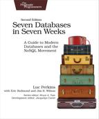
DynamoDB is, at root, a key-value store. But it’s a special key-value store in that it provides two types of key that you can choose on a table-by-table basis. You can use either a hash key (aka partition key) by itself or you can use a composite key that combines a hash key and a range key (aka sort key), as shown in the figure.
A hash key can be used to find items the same way you perform lookups in key-value databases such as HBase and Redis. You provide DynamoDB with a key and it checks the table to see if there’s an item associated with the key. Imagine fetching information about NFL teams that have won the Super Bowl using the year as the hash key. Or imagine retrieving information about an employee from a human resources database using the employee’s Social Security Number as the hash key.
A combination partition and sort key, however, enables you to find items on the basis of the hash key if you know it in advance or to find multiple items via a range query.
Imagine a table storing information about books in which each book item has two properties: a title (string) and the year published (number). In this case, you could use the title as a hash key and the year published as a range key, which would enable you to fetch book data if you already know the title or if you only know a range of years that you’re interested in.
Here’s an example aws command that creates a table with that key combination:
| | $ aws dynamodb create-table \ |
| | --table-name Books \ |
| | --attribute-definitions AttributeName=Title,AttributeType=S \ |
| | AttributeName=PublishYear,AttributeType=N \ |
| | --key-schema AttributeName=Title,KeyType=HASH \ |
| | AttributeName=PublishYear,KeyType=RANGE \ |
| | --provisioned-throughput ReadCapacityUnits=1,WriteCapacityUnits=1 |
A book like Moby Dick has been published many times since its initial run. The structure of our Book table would enable us to store many items with a title of Moby Dick and then fetch specific items on the basis of which year the edition was published. Let’s add some items to the table:
| | $ aws dynamodb put-item --table-name Books \ |
| | --item '{ |
| | "Title": {"S": "Moby Dick"}, |
| | "PublishYear": {"N": "1851"}, |
| | "ISBN": {"N": "12345"} |
| | }' |
| | $ aws dynamodb put-item --table-name Books \ |
| | --item '{ |
| | "Title": {"S": "Moby Dick"}, |
| | "PublishYear": {"N": "1971"}, |
| | "ISBN": {"N": "23456"}, |
| | "Note": {"S": "Out of print"} |
| | }' |
| | $ aws dynamodb put-item --table-name Books \ |
| | --item '{ |
| | "Title": {"S": "Moby Dick"}, |
| | "PublishYear": {"N": "2008"}, |
| | "ISBN": {"N": "34567"} |
| | }' |
You may have noticed that we supplied an ISBN attribute for each item without specifying that in the table definition. That’s okay because remember that we only need to specify key attributes when creating tables. This gives DynamoDB its relative schemalessness, which you can also see at work in the second item we created, which has a Note attribute while the others do not.
To see which books were published after the year 1980, for example, we could use a range query:
| | $ aws dynamodb query --table-name Books \ |
| | --expression-attribute-values '{ |
| | ":title": {"S": "Moby Dick"}, |
| | ":year": {"N": "1980"} |
| | }' \ |
| | --key-condition-expression 'Title = :title AND PublishYear > :year' |
| | { |
| | "Count": 1, |
| | "Items": [ |
| | { |
| | "PublishYear": { |
| | "N": "2008" |
| | }, |
| | "ISBN": { |
| | "N": "34567" |
| | }, |
| | "Title": { |
| | "S": "Moby Dick" |
| | } |
| | } |
| | ], |
| | "ScannedCount": 1, |
| | "ConsumedCapacity": null |
| | } |
With the query command, the --expression-attribute-values flag enables us to provide values for variables that we want to use as JSON. The --key-condition-expression flag enables us to provide an actual query string strongly reminiscent of SQL, in this case Title = :title AND PublishYear > :year (which becomes Title = "Moby Dick" AND PublishYear > 1900 via interpolation).
If you’ve used a SQL driver for a specific programming language, then you’ve probably constructed parameterized queries like this. As output, we got one of three books currently in the Books table, as expected.
Whenever you provide key condition expressions, you must match directly on the hash key (in this case Title = :title) and then you can optionally provide a query for the range key using one of these operators: =, >, <, >=, <=, BETWEEN, or begins_with. A BETWEEN a AND b expression is the direct equivalent of >= a AND <= b and begins_with enables you to create an expression like begins_with(Title, :str) where :str could be a string.
But what if we wanted our result set to include only, say, ISBN data? After all, we know that all the books are titled Moby Dick, so we may not need that as part of our result set. We can tailor that result set using attribute projection. On the command line, you can perform attribute projection using the --projection-expression flag, which enables you to specify a list of attributes that you want returned for each item. This query would return only the ISBN for each edition of Moby Dick published after 1900:
| | $ aws dynamodb query --table-name Books \ |
| | --expression-attribute-values \ |
| | '{":title": {"S": "Moby Dick"},":year": {"N": "1900"}}' \ |
| | --key-condition-expression \ |
| | 'Title = :title AND PublishYear > :year' \ |
| | --projection-expression 'ISBN' |
| | { |
| | "Count": 2, |
| | "Items": [ |
| | { |
| | "ISBN": { |
| | "N": "23456" |
| | } |
| | }, |
| | { |
| | "ISBN": { |
| | "N": "34567" |
| | } |
| | } |
| | ], |
| | "ScannedCount": 2, |
| | "ConsumedCapacity": null |
| | } |
If the attribute isn’t defined for a specific item, then an empty object will be returned. Remember that only one of our book items has a Note attribute. Here’s the result set when projecting for that attribute:
| | $ aws dynamodb query --table-name Books \ |
| | --expression-attribute-values \ |
| | '{":title": {"S": "Moby Dick"},":year": {"N": "1900"}}' \ |
| | --key-condition-expression \ |
| | 'Title = :title AND PublishYear > :year' \ |
| | --projection-expression 'Note' |
| | { |
| | "Count": 2, |
| | "Items": [ |
| | { |
| | "Note": { |
| | "S": "Out of print" |
| | } |
| | }, |
| | {} |
| | ], |
| | "ScannedCount": 2, |
| | "ConsumedCapacity": null |
| | } |
Note the empty object, {}, returned for one of the Items.
As you can see in this section, choosing the right key setup for any DynamoDB table is extremely important because that will determine how your application is able to discover the items it’s looking for. A good rule of thumb is this: If your application is built to know in advance where an item lives, then use just a hash key. An example here would be a user info database where you find items based on usernames already known to the application.
Spreading the Data Around: Partitioning in DynamoDB
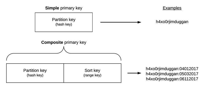
Behind the scenes, DynamoDB’s system for distributing item data across servers—partitions in DynamoDB parlance—is likely very complex. But from your perspective as a user it’s really fairly simple. You can see a basic visual illustration of data partitioning in the figure.
When you start writing data to a DynamoDB table, it begins filling in a first partition (partition 1 in the diagram). Eventually, that partition will fill up and data will start being distributed to partition 2, then at some point to partition 3, and so on out to N partitions. That N can be pretty much as large as you want; AWS provides no guidelines for limits to the number of partitions. The logic will simply repeat itself until you stop feeding data to the table.
How DynamoDB makes decisions about when to redistribute data between partitions isn’t something that Amazon makes transparent to the user. It just works. The only thing you have to worry about is ensuring as even a distribution of partition keys as possible, as laid out in the next section.
So just how big are these partitions? That’s determined by how much provisioned throughput you specify for the table. Think back to the read- and write-capacity units you specified in the create-table operation for the ShoppingCart table. There, one read capacity unit and one write capacity unit were specified. That provided the initial space allocation for the table. DynamoDB will add new partitions either when that first partition fills up or when you change your provisioned throughput settings in a way that’s incompatible with the current settings.
Location, Location, Location
As in any key-value store with limited querying capabilities, where you store things is an essential concern in DynamoDB and one that you should plan for from the get-go because it will have a huge impact on performance—and always remember that speedy, reliable performance is essentially the whole point of using DynamoDB.
As laid out in the previous section, DynamoDB uses a partition-based scheme for managing data within tables. You create a table and begin writing to it; over time, data is spread around across N partitions in an optimized way. But even though partitioning is automated, there are still some guidelines that you should follow when using tables.
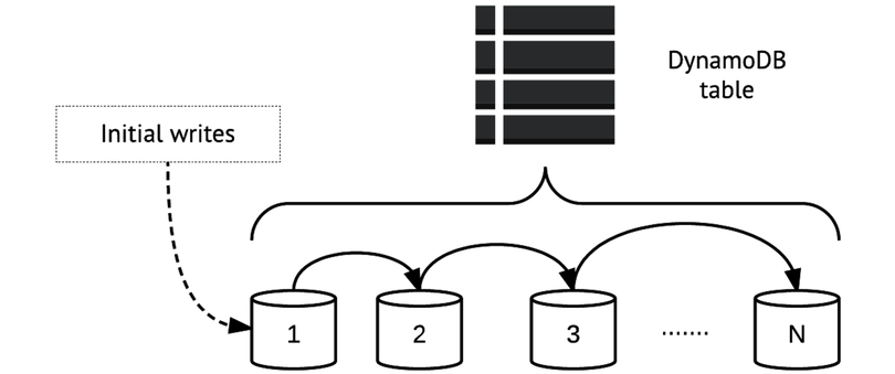
The tricky part of partitioning is it’s possible to create an uneven distribution of items across partitions. For a basic illustration, see the figure.
DynamoDB always performs best—in terms of read and write speed—when access to partition keys is balanced. In this illustration, the size of each upward-facing arrow shows how intensively each partition is accessed. Partitions 2 and 4 here take significantly more traffic than partitions 1, 3, and 5, making partitions 2 and 4 so-called “hotspots.” The presence of hotspots is likely to detract from performance for all partitions and should be avoided whenever possible.
In general, you can crystallize best practices for DynamoDB performance into just a few basic maxims.
First, if you’re using a hash key as your partition key, you should always strive for a data model in which the application knows the key in advance because this will enable you to target the item directly rather than relying on range and other queries. You should make the hash key something meaningful—for example, the username of each user in a CRM table, the device ID for each sensor in an “Internet of Things” table (more on that in Day 2), or a UUID-based transaction identifier in an inventory table. When working with key-value stores, this is simply the nature of the beast, and DynamoDB is no different here.
Second, because the partition key determines where data is stored, you should use partition keys that don’t cluster around just a few values. If you had a partition key with only a few possible values, for example good, bad, and ugly, you would produce hotspots around those values.
Third, in cases where you need to use a composite key—a hash key plus a range key—you should opt for fewer partition keys and more range keys. This is best illustrated with an example. Let’s say that you’re a video game company that makes the game Bonestorm. Bonestorm has over a million players and you want to store daily total stats for each player on each day that they play the game. You could use username/date composite keys that look like this:
| | h4x0rjimduggan:04012017 |
| | h4x0rjimduggan:05032017 |
| | pitythefool:11092016 |
| | pitythefool:07082016 |
A less-optimal strategy here would be to make the date the hash key and usernames the sort key. Because there are far more users than there are dates—by a favor of thousands—the number of items with the same hash key would be much higher.
As is always the case with key-value stores, even a “key-value plus” store like DynamoDB, your application needs to be smart about how it stores data and how keys are structured. One of the great things about RDBMSs that we’ve discovered after years of experimenting with NoSQL databases is just how flexible they can be. DynamoDB is more flexible than other key-value stores—composite keys provide for that—but careful planning, before you write even your first items, is nonetheless essential.
Tables Within Tables: Indexes in DynamoDB
The last core component of DynamoDB that we’ll explore on Day 1 is indexing. Indexes are essentially mini tables that enable you to look up data more efficiently. Indexes in DynamoDB work much like they do in relational systems, storing lists of keys for objects based on some set of criteria.
Indexes usually offer a crucial performance boost because they prevent you from needing to run some of your more expensive queries. Instead of scanning an entire table and then selecting a subset of the results, which is almost never a good idea, you can query or scan the index instead. The price you pay for indexes is that they take up additional disk space. Whether or not that price is worth the performance boost depends on your use case and is difficult to decide in advance without knowing a lot of particulars. In DynamoDB, indexes come in two flavors: local and global.
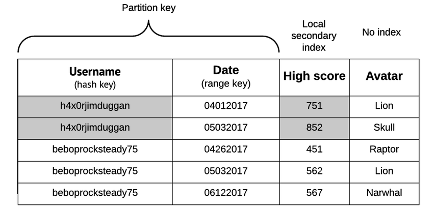
Local Secondary Indexes
Local secondary indexes (LSIs) let you query or scan attributes outside of your primary hash and sort key. The “local” in “local secondary index” means among items sharing a partition key. You can see an example of this in the following figure. Here, a local secondary index is created for the High Score attribute. The LSI on the High Score attribute here means that we can perform scans or queries related to high scores for a specific user.
Here’s an example range query for the HighScore attribute that shows all of the dates on which the player h4x0rjimduggan scored over 800 points:
| | $ aws dynamodb query --table-name BonestormData \ |
| | --expression-attribute-values \ |
| | '{":user": {"S": "h4x0rjimduggan"},":score": {"N": "800"}}' \ |
| | --key-condition-expression \ |
| | 'Username = :user AND HighScore > :score' \ |
| | --projection-expression 'Date' |
Always bear in mind that LSIs can’t be modified after a table has been created, so be extra careful to plan for them in advance (or, even better, thoroughly test different indexing models in development).
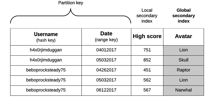
Global Secondary Indexes
Global secondary indexes (GSIs) are indexes that aren’t restricted to items with the same partition key. The “global” here essentially means “any attribute in the table.” See the figure for an example. You can find any items in the table using the Avatar attribute.
Here’s an example query that finds all items for which the Avatar field equals Lion and returns the Username and Date for each of those items:
| | $ aws dynamodb query --table-name BonestormData \ |
| | --expression-attribute-values \ |
| | '{":avatar": {"S": "Lion"}}' \ |
| | --key-condition-expression \ |
| | 'Avatar = :avatar' \ |
| | --projection-expression 'Username, Date' |
An important thing to note is that GSIs can be modified after a table has been created, whereas LSIs cannot. This makes it somewhat less crucial to get your GSIs right from the get-go, but it’s still never a bad idea to make a thorough indexing plan in advance.
Day 1 Wrap-Up
Here on Day 1 we did a lot of conceptual exploration, from supported data types to indexing to the core philosophy of DynamoDB, but we didn’t really do anything all that exciting with DynamoDB. That will change on Day 2, when we’ll embark on one of the most ambitious practical projects in this book, building a streaming data pipeline that ties together multiple AWS services to create a streaming data pipeline that uses DynamoDB as a persistent data store.
Day 1 Homework
Find
-
DynamoDB does have a specific formula that’s used to calculate the number of partitions for a table. Do some Googling and find that formula.
-
Browse the documentation for the DynamoDB streams feature.[48]
-
We mentioned limits for things like item size (400 KB per item). Read the Limits in DynamoDB documentation[49] to see which other limitations apply when using DynamoDB so that you don’t unknowingly overstep any bounds.
Do
-
Using the formula you found for calculating the number of partitions used for a table, calculate how many partitions would be used for a table holding 100 GB of data and assigned 2000 RCUs and 3000 WCUs.
-
If you were storing tweets in DynamoDB, how would you do so using DynamoDB’s supported data types?
-
In addition to PutItem operations, DynamoDB also offers update item operations that enable you to modify an item if a conditional expression is satisfied. Take a look at the documentation for conditional expressions[50] and perform a conditional update operation on an item in the ShoppingCart table.