Anti-debugging is a natural occurrence that should be expected; as soon as people started reversing applications it was only a matter of time before other people started trying to make it harder, implausible or even impossible for someone to reverse their application. Anti-debugging, like reverse engineering or coding in assembly, is an art form. The trick of course is to try to stop the person reversing the application. However, in most instances these attempts range from the absurdly lame to the truly difficult. At first it may be your presumption that only malicious software would seek to impede your reversing progress, but really you will find it everywhere and indeed there are legitimate jobs out there just for people to create such anti-reversing technologies, especially in the video game industry. In this chapter, what we hope to do is write a fairly comprehensive overview of anti-debugging and anti-disassembly techniques. Make no mistake—these tricks and techniques are designed to make your life and job more difficult, and in some instances there really is no good solution to getting around the problem presented. However, it is important to know and remember one thing: Given enough time and motivation, the reverse engineer always wins.

First, if we really want to understand anti-reversing, then a little knowledge of exactly how debugging and disassembling is done would be helpful. This of course is not meant to be an all-encompassing perspective on the art, but rather a brief introduction to how it works, with the intent of using that knowledge as leverage to understanding anti-reversing techniques.

To really understand debugging, a brief tour of the various interrupts and debug registers is necessary, especially in regards to what state changes occur in the process. The Intel Software Developers Manual is once again the best place for reference in this regards, as it goes much deeper into details than I can. However, basically the IA-32 platform handles debugging through one of a couple of means.

First, the debug registers. There are eight debug registers supporting the ability to monitor up to four addresses. The registers themselves are accessed through variants of the MOV instruction with the debug registers potentially serving as either the destination or source operands. It should be known that accessing the registers is a privileged process requiring ring-0 privileges, which of course is a limiting feature but considering the power they give it makes sense. For each breakpoint, it is necessary to specify the address in question, the length of the location (ranging between a byte and a dword), a handler when a debug exception is generated and finally whether this breakpoint is even enabled. The first three debug registers, DR0 through DR3 can contain three 32-bit addresses that define the address where breakpoints should occur. The next two debug registers, DR4 and DR5 respectively, have alternating roles depending on mode of operation. When the debugging extensions (DE) flag is set in control register 4 (CR4), DR4 and DR5 are reserved and cause an invalid-opcode exception when an attempt to reference them is made. If the flag is unset, then DR4 and DR5 are instead aliases for debug registers 6 and 7.

Debug register 6 (DR6), is also known as the debug status register and indicates the results of conditional checks at the time of the last debug exception. DR6 is accessed as a bit pattern, with bits zero through three being related to the first three debug registers. Each of these bits indicates which breakpoint condition was met and caused a debug exception to be generated. Bit 13 of DR6 when set indicates that the next instruction references a debug register and is used in conjunction with a portion of DR7, which we will describe momentarily. Bit 14 is perhaps the most interesting for our purposes; it indicates when set that the processor is in single-step mode, which is yet another concept we will introduce momentarily. Finally in use is bit 15, which indicates that a debug exception was raised as a result of a task switch when the debug trap flag was set. Finally, we arrive at debug register 7, or DR7 as you might have guessed. This is a very interesting register to hackers of all kinds as it’s also known as the debug control register and like DR6 is interpreted as a bit field. The first byte of this register corresponds to whether a breakpoint is active, and if so its scope. Bits zero, two, four and six determine whether a debug register is enabled or not, with bits one, three, five and seven corresponding to the same breakpoints but on a global scope. The scope in this instance is defined as whether the breakpoint persists through task switches, with globally enabled breakpoints being available to all tasks. In later versions of the processor, according to the Intel manual, bits eight and nine are not supported. However traditionally they provide the ability to determine the exact instruction that caused the breakpoint event. Next we have bit 13; this is an interesting bit as it allows for breaking before accesses to the debug registers themselves. Finally we have bits 16 through 31. These bits determine what types of access cause a breakpoint, and what the length of the data at the address is. When the DE flag in CR4 is set, bits 16 to 17, 20 to 21, 24 to 25 and 28 to 29 are interpreted in the following manner:

00 – Break on execution
01 – Break on write
10 – Break on I/O read or writes
11 – Break on read and writes but not instruction fetches

However, when the DE flag is not set the interpretation remains the same except for values of 10 which are undefined. Bits 18 to 19, 22 to 23, 26 to 27 and 30 to 31 correspond to the lengths of the various breakpoints with a value of 00 indicating that the length is 1, and 01 indicating a 2-byte length. 10 is undefined on 32-bit platforms, with it indicating a length of 8 bytes on 64-bit processors. Finally, as you might have deduced, a value of 11 indicates that the length in question is 4 bytes in length.

Now it may seem a little confusing trying to tie all these bit sequences together with DR0 to DR3, but it really isn’t. Each 2-bit combination corresponds to a given sequential register in the range of DR0 through DR3. These lengths must be aligned on certain boundaries dependent on their size—for instance 16-bit values need to be on word boundaries and 32-bit ones on double-word boundaries. This is enforced by the processor by masking the relevant low-order bits of the address; thus an unaligned address will not yield performance as expected. An exception is generated if any addresses in the range of the starting address plus its length are accessed, effectively allowing for unaligned breakpoints by using two breakpoints; each breakpoint is appropriately aligned and between the two of them they cover the length in question. Now one last note of interest here—when the breakpoint access type is execution only, then the length specified should be set to 00; any other value results in undefined behavior.

Now we’ve mentioned debug exceptions throughout the description of the registers, but we haven’t really done anything beyond mention them. The IA-32 processor has an interrupt vector specified in the interrupt descriptor table which was described previously in Chapter 2. Of these, the processor dedicates two interrupt vectors to these exceptions. These two interrupts are one and three, which are the debug and breakpoint exceptions, respectively. The debug exception, or INT 1, is generated by multiple events and DR6 and DR7 should be consulted to determine what type of event occurred exactly. In the process of an exception there are two general classes, faults and traps. Essentially, the difference between the two classes is whether the instruction that generated the interrupt was executed or not by the time the handler gets control. In faults, control is handed to the handler first, whereas in traps execution control is passed to the handler after the instruction that caused the exception is generated. Of these two classes, we have several different conditions that fall into the classes: instruction breakpoint, data and I/O breakpoint, general-detect, single-step and task-switch conditions. Of these the instruction breakpoint, general-detect and arguably task-switch conditions are fault class, while data and I/O breakpoint and single-step conditions are trap class.

Instruction breakpoint class conditions are the highest priority exceptions and occur when an instruction at an address referenced in DR0 to DR3 is attempted to be executed. We say that these exceptions are the highest priority meaning that they receive service first; however, there are instances where these events may not even be triggered We’ll delve into that a bit later though. Now if you recall in the description of the EFLAGs register earlier, there was the resume flag in present. The problem is that it’s possible for a debug exception to be re-raised as a result of this exception being a trap-class exception. This is where the resume flag comes into play, as it prevents looping of the debug exception. We’ll cover this also shortly when we start to delve into specific methodology. The other fault class condition is the general-detect condition; this is raised when the relevant bit in DR7 is set, protecting access to the debug registers.

Data and I/O breakpoints are trap-class conditions and are caused by data accesses of addresses in DR0 to DR3. Data accesses are essentially any condition that’s not an execution attempt. The IA-32 processor contains an interesting quirk in that trap-class events occur after the instruction that caused them was executed. For instance, suppose you set a write breakpoint on address X whose value is 0 and then the application modifies address X, setting its value to 1. When the exception handler receives control, the value at address X will be 1, not 0. The Intel manuals suggest that applications that want to be able to interact with the original value should save it at the time of the breakpoint, although doing so creates an interesting but off-topic synchronization issue. Even more, these breakpoints, like instruction breakpoints, are not always exact; for instance, repeated execution of certain SIMD instructions can cause the exceptions to be raised until the end of the second iteration.

Single-step exceptions are also trap-class conditions, and are one of the more common conditions encountered when debugging. These conditions are caused when the trap flag in the EFLAGs register is set. Just like every other type of exception, single stepping comes with its own quirks. For instance, generally speaking the trap flag is not modified in the process of performing various tasks; however, certain instructions like software interrupts and INTO instructions do clear the trap flag. This effectively means that, in order to maintain control, a debugger has to emulate these instructions and cannot directly execute them, that is if they wish to continue inspiring single-step exceptions. Finally, task-switch exceptions occur after a task switch if the trap flag in the new tasks TSS is set; the exception is raised after the task-switch but prior to the first instruction in the new task.

Now, in addition to INT 1, there is also the breakpoint exception or INT 3. The breakpoint exception is interesting in that it allows for extension of breakpoints past the number supported by the debug registers. However, it requires modifying memory, an Achilles heel that we will talk about exploiting later. For now, all we really need to know is that it exists.

Upon hearing all of this, an inspired reader with a good imagination might already begin to see the conditions that could be checked for and ways that interruptions might be avoided. However, people don’t purchase nonfiction books to inspire their imagination but rather to learn facts, so we’ll cover some of the complications that can occur in the rest of the chapter. We will explore mostly ring-3 based implementations of circumventing both disassembly and debugging, but to spice things up some we will also touch on some ring-0 based concepts.

Because this is a somewhat tricky subject which can be difficult to explain exactly, especially within the constraints of a single chapter, we’re going to take the following approach. I’ve written a simple application, a silly network RPC server and client. What we’re going to do is take this (the server side component) application and harden it to reversing a bit, or rather do as much as we can within the constraints. Thus, we will have two products: the original program and the one we’ve hardened. The idea here is that we’re going to reverse the anti-RCE process and, by making one ourselves and looking at the generated code, when you do eventually run across this sort of stuff, you’ll have some concept of what’s going on and how to get around it. The example codes we will be using for this chapter are available for download from the Syngress website. We will not be looking at the client side of the application, and it is there simply for you to experiment with, and for me to verify that everything is working as expected.

So without any further ado, let’s take a brief look at the application prior to doing anything to it, so you have some idea of what it started off looking like. Figure 6.1 shows the relevant section of the control-flow graph that’s generated when you go to View > Graphs > Control Flow, or if you hit F12, the options hotkey. This isn’t the full graph, as it’s not necessary and trying to fit it into a page was problematic. Basically, I want you just to get an idea of what we’re looking at. However, I highly encourage you to download the source, compile it and look it over.

Figure 6.1. Control Flow Graph

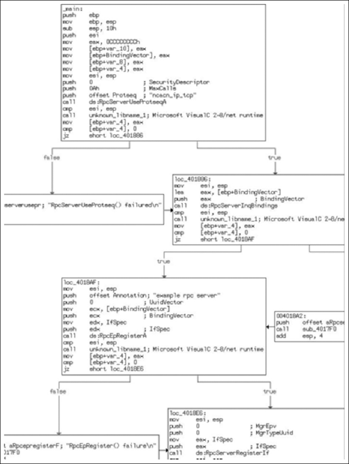
As you can see, this is obviously an application dealing with RPC in some form, and when we take a closer look it becomes clear that it’s intended to be the server component, as one can tell just by the API calls. As you examine the code, take note that there are multiple string constants, that there is really no attempt to obfuscate what the application is doing and so on. Now, let’s change that! If you feel a little lost at this point, pull the code down and take a closer look at it to get a better feel for it, as this is a chapter about anti-reversing, not about coding an RPC server and I really can’t delve into the details much further.

As we noted earlier, there is very little doubt about what is going on in this program, or at least what appears to be going on. (One should be careful about forming conclusions in regards to the application’s purpose with such a small preview; however, in this case, what we see is what we get.) Let’s start off with one of the simpler, although more effective, techniques and obfuscate the code a bit.

These types of techniques are common and really are something you should just accept as the normal routine; sans any other types of security, they generally won’t pose much of a problem for you. What we’re actually trying to do here is raise the bar as to who can read the code. You see, a decent percentage of people calling themselves “reverse engineers” or working as “incident responders,” really aren’t. Some of them can do little more than extract readable strings from the binary, others just read API calls, while some will take a guess of intent based on data in the imports section. An often-used trick—especially when dealing with packed binaries— is to modify some aspect of the binary so that if someone tries to dump the image straight from memory it will be corrupted.

Taking this all into account, let’s take a look at the newly modified main routine in Figure 6.2.

Figure 6.2. Modified Main Routine

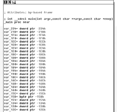
Looking at just the entry point reveals that this new binary could be significantly more complex, just by the number of local variables now present. Of course, we are also looking at different views of the code, so this isn’t quite as obvious as when we reach the first sets of instructions (see Figure 6.3).

Figure 6.3. First Instructions

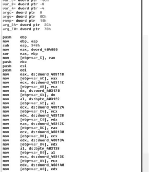
The trend in change of the code continues as we note that, where once there was the start of RPC calls, we now have a long series of byte copies from the data segment onto the stack. You may note that the stack is declining while the data index is increasing; this is typical of things like string constants initializing a stack variable. We’ll come back and look at this in a moment. However, before we delve into the changes I want you to be able to see and get a feel for the differences in the program, as seen in Figure 6.4.

Figure 6.4. Differences in the Program

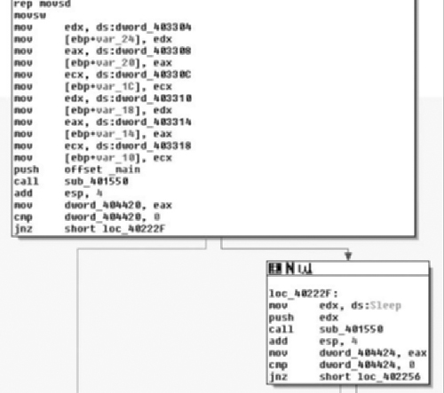
Continuing down the code, we finally get to the first “real” portion of code, which is a call to the function sub_40155. There are two calls to it, the first passing the address of the main function in as an argument, the second passing in the address of the kernel32 function Sleep( ). Now that we have some idea of what we’re getting ourselves into, let’s take a bird’s-eye view of the code (Figure 6.5) and see how crazy the structure of the application might be.

Figure 6.5. Complicated Structure of Application

And here we have it—no matter how awkward the code initially appears, it exhibits fairly typical structures, still showing a basic Boolean logic to its overall composition. Most of the complexity appears to be towards the start, and then we see a simple series of if () { if () [...] else [...] } else [..] structures. Notice the first error branches to the right, whereas the second error branches off to the left, continuing on down to process termination.

Great! Now that we have some idea of what we’re working with, let’s go back and get a better idea of how exactly it changed and see if we can figure out how this little puzzle fits together, starting with that long series of copies from the data section to the stack. Starting at the beginning of the data, we have address loc_403118, so let’s jump there and see what we can determine (Figure 6.6).

Figure 6.6. address loc_403118

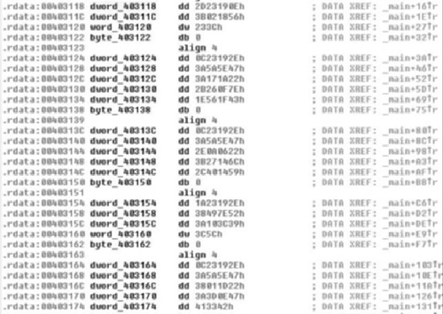
As we examine the data that initially is referenced in the main( ) function, it becomes obvious that they are not ASCII characters. However, they appear to be NULL terminated, further supporting the idea of string constant initialization of local variables. Furthermore, we can take note that the data has some repeating patterns, for instance, look at how many sequences start with the bytes 0x0C2319. This may be indicative of weak encryption. We really won’t be able to tell for sure until we get to a section of code that interacts with this data. We’ll shelve the idea for now, but we can speculate that the program once accomplished a great deal with RPC and had many string constants, and now contains a bunch of random NULL terminated data that appears to at least have a repeating first three characters in most of the cases.

Now, knowing that there is not a lot we can do at the present time about the apparently encrypted data, unless we’re willing to track down where the data gets used, we’ll move on to the next portion and let the order of operations occur sequentially. Next up, we have the function sub_401550 (Figure 6.7).

Figure 6.7. Function sub_401550

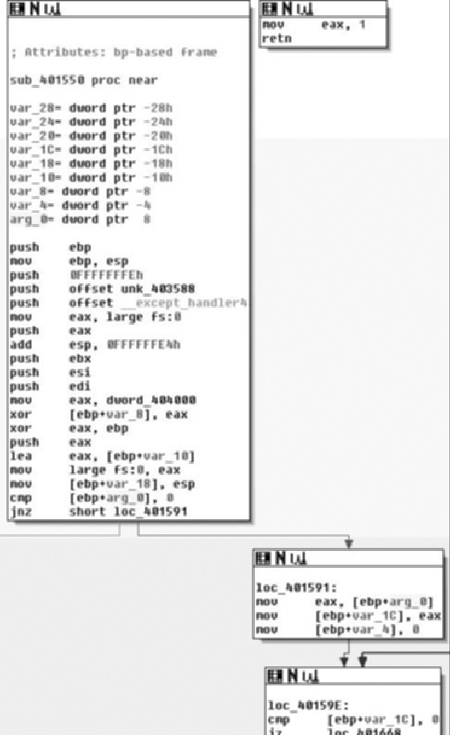
As we examine the entrance of sub_401550, we see a function that’s a bit more normal looking than main( ). As you may recall, in the first part of main( ) this is invoked twice, once with an argument of the address of main and once with a pointer to Sleep( ). The user portion of the code starts at the cmp instruction testing arg_0 against 0 towards the end of the first box. One thing to note in the compiler-generated code is that there is an exception handler setup.

So the first real thing we see is that the argument is tested against 0, or rather the pointer is checked against NULL, if it is, we branch off to the left presumably towards an abnormal termination. If the pointer is non-NULL then in the branch to the right, at loc_401591 we see the variable var_1C is initialized to the value of the routines parameter and var_4 is initialized to 0 (Figure 6.8).

Figure 6.8. var_4 Is Initialized to 0

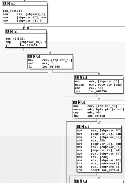
Continuing down through the function, we arrive at loc_40159E, which appears to also start the mark of a loop. This loop is made more obvious if you’re looking at the function in its entirety in the graphs; just remember this as being the loop back point, as you can tell by the arrow coming from the upper right back to loc_40159E. As far as functionality, what we see in this box is that the pointer copy of the routine parameter is tested against NULL again and then if it is, a branch occurs to the left, otherwise the routine branches to the right. From there we move down to the third box where the var_1C pointer is decremented by one and tested against zero, again branching to the left if the condition is true. From there, in the fourth box down we see the pointer dereferenced and checked against the byte 0x5A; if a match is found, then it moves to the fifth box, if not it branches to the left.

If there was a match, the byte prior to this is checked against the value 0x4D, meaning that we’re looking for the 16-bit sequence 0x4D5A. As you may recall, this corresponds to the ASCII letters MZ, which is how a DOS header starts. Without looking further, we can make an educated guess that the function appears to be walking backwards through memory attempting to find the beginning of the file—this also explains the use of SHE as in theory it would be possible to touch bad memory and crash. We’ll continue looking through the routine though; it would be bad practice to just presume based on so little.

Next, in the final visible box, if a match against 0x4D5A was found, the pointer is copied into var_20, and then incremented by 0x3B and this new pointer is copied into var_24. Finally, what we see next is the var_1C, or the pointer to the MZ summed with the value from var_24 (var_1C + 0x3B) plus two. This incidentally corresponds to the offset of the PE header in the DOS header and it would appear that the final box attempts to find the start of the PE header and then compares that pointer to arg_0 and branches dependent on result, presumably towards another abnormal exit (see Figure 6.9).

Figure 6.9. Match Against 0x4D5A

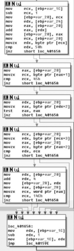
Moving into the next section, we see the same theme continued; in the first box we see a comparison against 0x50 followed by a check for 0x45. This in turn means it’s looking for 0x4550. If there is a match, the next two boxes check to see if the sequence is followed by two zero bytes, meaning a full match thus far requires the sequence 0x45500000, or PE\0\0, which is of course the magic value for a PE header. Finally, as the last check in this section we see that they test against the value 0x14C, which corresponds to IMAGE_FILE_MACHINE_I386. All of this and previous sections make sense and it appears that the argument to the routine is a pointer that is an offset into an executable image. Given that input, the routine walks backwards through memory attempting to identify the start of the DOS header. Once found, it uses this information to locate the PE header and performs other light verifications of the data.

As we can see in the second to last section of code, if a total match is found, we branch off to the left, and if not then we jump to the location loc_40165A, which takes the pointer, decrements it by one and repeats the loop. Now that we know the body of the routine, let’s examine the branches we haven’t yet looked at and also take a look at the return value.

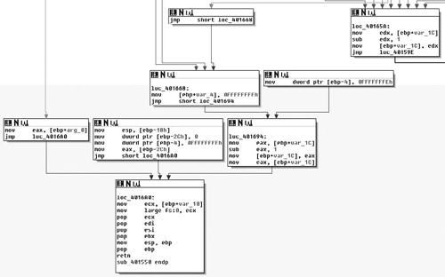
In Figure 6.10, starting from the top right, at loc_40165A, we see that if a match was indeed found then we jump to loc_401668, which modifies var_4 and then passes control to loc_401694 which retrieves the base address, decrements it by one and then hands control to the cleanup portions of the routine. This means that the return value is a pointer to the base address of the image in question. We also see, on the far left, the result of the initial test of arg_0, which if it was NULL is the value returned. Thus we can conclude that, given a pointer, this routine finds its base address, returning that pointer or NULL on error.

Figure 6.10. Jump to loc_401668

Now, after reviewing this routine, let’s take a look at the main( ) routine again and see what becomes apparent. We’ve renamed this routine to FindBaseAddr( ) as that is the functionality it provides (Figure 6.11).

Figure 6.11. FindBaseAddr()

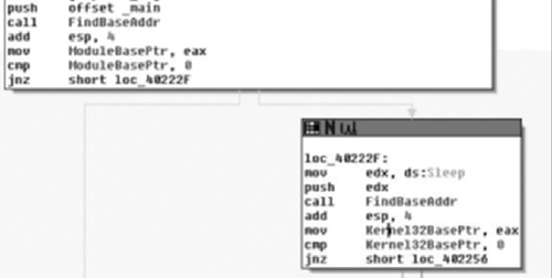
Updating this information in IDA, we can plainly see that these two invocations find the base address of the current module and the Kernel32 module, respectively. We’ve updated the variable names to reflect this, calling the pointers the ModuleBasePtr and Kernel32BasePtr for each. We now can make a guess at what is going on, as it’s not typical for code to manually find its own base through this method, and totally unnecessary to find Kernel32. We can probably safely bet this is an attempt at obfuscating library calls. Following the routine’s return, we see both pointers tested against NULL, branching to the left if this is true. Let’s not consider these error branches yet, and examine the scenario where both calls to FindBaseAddr( ) succeed. (See Figure 6.12).

Figure 6.12. loc_402256

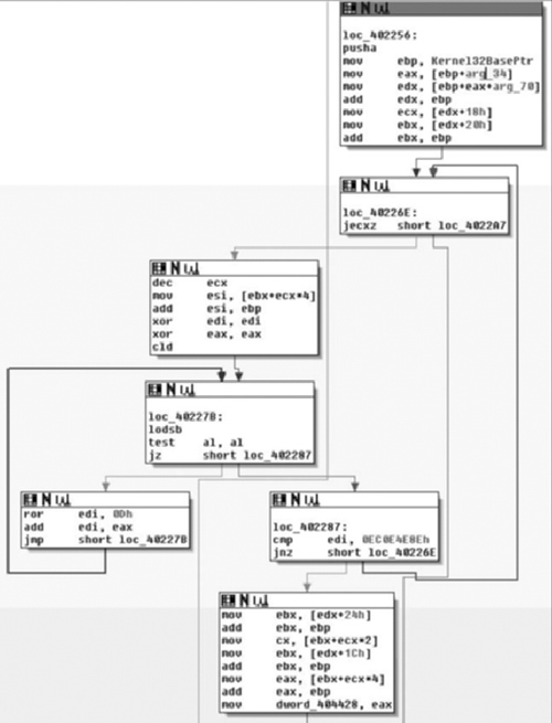
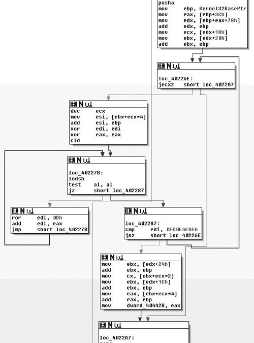
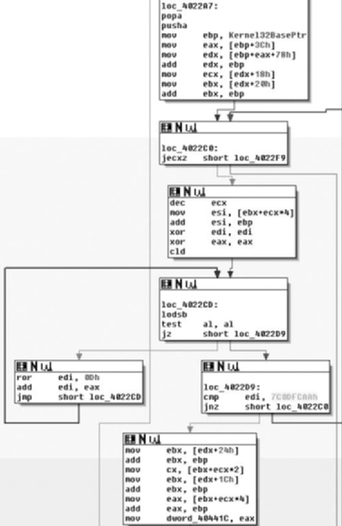
Moving on through the code, at loc_402256, which is where control is handed after the check of the return value from the second call to FindBaseAddr( ) if the base address for kernel32.dll was found successfully, we first see that a pusha instruction is executed (Figure 6.13). Some may argue with me on this, but there are instructions like pusha that I don’t see the compiler generate often and so I often suspect when looking at that code that it may have been hand-written. I know, because I wrote the source in this case, that this is true, but it’s an observation that I think is generally true; your mileage may vary of course.

Figure 6.13. Viewing under a Disassembler

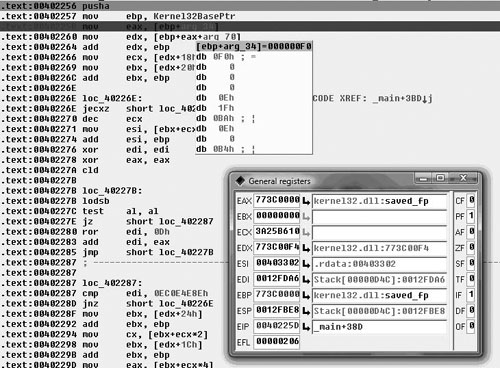
At any rate, we see the Kernel32 base pointer retrieved and it has arg_34 and arg_70 added to the base; we then see offsets 0x18 and 0x20 retrieved from that offset and 0x20 is added to the base pointer. From this point, we could make a guess at what the function does based on what we’ve already seen and the parameters and offsets being worked with. Plus, if you’ve done any Windows exploitation, the entire code sequence should look familiar to you, but we’ll take a look a little further because something interesting occurred here.

If you look at the first box, loc_402256, you’ll notice that arg_34 and arg_70 are used. There are two things that make this odd: the first is that we’re inside the main( ) routine, and there was no arg_34 or arg_70. If there were, these should be expressed as offsets from argv or envp. The second is that these values are only read from, so by looking at this statically we’re not even positive what these offsets will be exactly. This is actually a pretty good thing for the person employing anti-reversing; in order for me to really know what’s going on in that section of code, I’m going to need to look at it in a debugger and so, unless I skip this part, static analysis stops. In my opinion, what makes this good is that now they can actually take an active role in attempting to complicate the reverser’s life, as opposed to a passive/static role that can be achieved when being viewed under a disassembler. (See Figure 6.13).

When we look at it in the debugger, we find that this view is not all that much more helpful. However, if we double click on arg_34 and view that memory, what’s going on becomes a little more clear (Figure 6.14).

Figure 6.14. arg_34

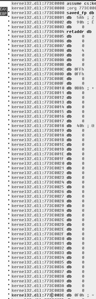
When we view the pointer that IDA is calling arg_34, it becomes clear that it’s an offset from the base of Kernel32.dll, specifically the offset 0x3C, which as you may recall from FindBaseAddr( ) is the offset from the base to where the offset to the PE header is specified. This makes sense, a lot more sense than arg_34 implies. Now you may think that this is a great way to obfuscate intent, and indeed it works with limited success and serves mostly as an annoyance. However, it should be noted that other debuggers—such as OllyDBG—may not have the same issues. For instance, Figure 6.15 shows a screenshot from the ImmunitySec debugger, which is a rebranded OllyDBG with Python glued to it.

Figure 6.15. ImmunitySec Debugger

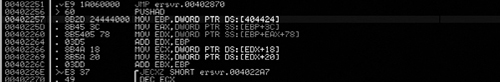
As you can see here, the code is represented correctly in this debugger and its purpose is pretty clear. The main reason this occurs in IDA is because the code fiddles with the EBP register (generally speaking, another tell-tale sign of inline assembly). This in turn causes IDA to confuse the offset and think it’s a function parameter. Another reason that could have a noticeable impact, although it is quite likely that fiddling with EBP was enough, is that this was actually a function that was inlined. Either way, after a brief step into the debugger, we know that these two mov’s are actually taking offsets 0x3C and 0x78 from the Kernel32 base, respectively. (See Figure 6.16).

Figure 6.16. Offsets 0x3C and 0x78 from the Kernel32 Base

At any rate, fixing the misrepresentation by IDA is easy enough; by right-clicking on the variable name we are prompted with a list of different representations, the first option being the correct one. Thus, we really didn’t need to use the debugger. Considering the rest of the code here, this is actually a fairly familiar sequence of code that, as far as the author is aware of, employs a technique first publicly divulged by a Polish hacker group named the Last Stage of Delirium (LSD) and then later expanded upon and reiterated upon in a paper by Skape and the nologin crew, “Understanding Win32 Shellcode.” What we see is that the PE header is found at offset 0x3C, then this offset plus the base plus 0x78 yields the Exports data directory. The rest of the code is simply iterating over Exports and taking the names and hashing them with a ror instruction. This result is then compared with another 4-byte hash and, if it matches the export in question, has been found.

In other words, this is just a position independent way of finding a DLL’s export without depending on any other APIs. This is often used during the “bootstrapping” process of shellcode. It’s typically used to find the address of functions like LoadLibrary( ) and GetProcAddress( ). Consequently, if you look at loc_402287 you will see a cmp of EDI with the constant value 0x0EC0E4E8E. This is the hash that this code is looking for and if you simply pop it into Google (or run it through a debugger) you would find that this is the hash that corresponds to LoadLibraryA( ). The code in the second to last box from the bottom is where a match was found, and thus we can rename the variable dword_404428 to be a pointer to LoadLibraryA( ) and move on. I didn’t really dig into the details of the algorithm here, mostly due to space requirements, but if you’re interested I strongly advise that you look up either the paper by Skape or LSD.

Moving along, we notice a startling familiarity in the next section of code (Figure 6.17), almost to the point that you may wonder if I reposted the wrong image! I assure you I did not. What we see here is another walk through Kernel32 in the same manner in an attempt to find another exported function. This time the hash in question can be found at loc_4022D9 and has a value of 0x7C0DFCAA. Once again, either via Google or a debugger, you would find pretty quickly that this is the hash value for the GetProcAddress( ) function; thus this section of code just locates that pointer, and saves it at dword_40441C, which we will rename to GetProcAddressPtr. One other thing the reader might note is that this section of code did not exhibit the same oddity as earlier when extracting offsets 0x3C and 0x78. This is simply the result of my changing its representation already.

Figure 6.17. Kernel32

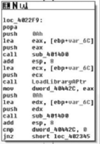
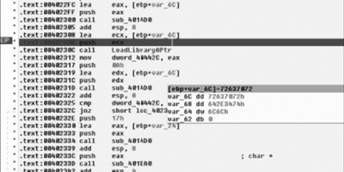
Immediately following the previous code, in Figure 6.18, we find loc_4022F9 in which we can see a call to another new subroutine whose return value is stored in var_6C. Following that we see a call to LoadLibraryA( ) so it’s a pretty good guess that this likely decrypts or decodes some of that stack data we looked at first. Furthermore, we find that we’ll save the return value from LoadLibraryA( ) in dword_40442C. Finally, we get another clue as to what to expect for the encryption/encoding, as after the usage of the string we see that a call to sub_4014D0 is made again with the same argument of var_6C, at least implying that we’re probably going to be looking at a symmetric cipher of some sort. We’ll take a brief look at this implementation just to get an idea of what’s going on in there, but once you’ve confirmed that it’s just some sort of string obfuscation scheme that encrypts/decrypts itself, it’s typically fastest to simply let it do its thing and copy the results out.

Figure 6.18. loc_4022F9

That said, you should probably at least read the source of the function you’re going to step over to ensure it does what you think it does; we’ll largely leave this as an exercise for the reader however, as the book gains little from a detailed analysis of the crypto employed and it would take up a significant amount of space in a chapter that’s already tight. Plus, it’s trivial but not trite, so it will work out as a good educational exercise for the inspired reader.

Reloading the debugger, letting the program do the hard work and decrypt the string for us, what we see post calling sub_4014D0 is the hex sequence seen in Figure 6.19. If you look it up, this corresponds to the ASCII mapping for the NULL terminated string “rpcrt4. dll”—the library required to make RPC calls in Windows. This makes sense, of course, given that we know this to be an RPC server from our earlier analysis. This also largely pieces the puzzle together, as we can likely guess that the purpose of the GetProcAddress( ) pointer. Once again, to conserve space and leave something to do for the reader, we’ll leave the rest as an exercise.

Figure 6.19. Reloading the Debugger

To review the techniques described in this chapter, we’ve seen the code base make-up change drastically and the complexity of the program increase rapidly as well. We’ve seen how easy it is to remove the string constants and similar. The interested reader who finds this particular section interesting might enjoy reading more about things like overwriting pointers in the Import Address Table (IAT), or copying system functions into user allocated space to avoid breakpoints on functions. Another technique that originated from the virus-writing world is a technique called entry point obscuring or EPO. Traditional viruses would modify the entry point in the executable header and typically append themselves to the executable file. This of course yielded a tell-tale sign of infection and gave anti-virus an easy target. As a result, EPO viruses started to appear. EPO viruses, instead of modifying an entry point, will scan the executable section for a jmp or similar and modify that to hand control to the virus elsewhere. This same technique could be used to take advantage of the fact that IA-32 machines have limited debugging support by entering into system libraries 5 to 10 bytes into the function instead of at its original entry point.