In this chapter we will introduce basic items, providing a brief introduction to assembly and the Intel architecture processor and covering various other concepts that will help ease you into the subject matter. This book focuses on 32-bit Intel architecture (IA-32) assembly and deals with both the Windows and Linux operating systems. The reader is expected to be at least mildly familiar with IA-32 assembly (although the architecture and instruction set are covered to some degree in this chapter), and a firm grasp of C/C++ is expected. The point of this chapter is simply to give those who are either unfamiliar with or a little rusty on the subjects presented in this book a base to work from, and to provide a basic reference point to which the authors can refer should it be deemed necessary.

Assembly is an interesting method for communicating with computers; Donald Knuth once said that “Science is what we understand well enough to explain to a computer. Art is everything else we do.” To me, this truth is most prevalent in assembly programming, because in so many areas as you write assembly you find yourself doing things like abusing instructions by using them for something other than their intended purpose (for instance, using the load effective address (LEA) instruction to do something other than pointer arithmetic). But what is assembly exactly? Assembly refers to the use of instruction mnemonics that have a direct one-to-one mapping with the processor’s instruction set; that is to say, there are no more layers of abstraction between your code and the processor: what you write is what it gets (although there are some exceptions to this on some platforms where the assembler exports pseudo-instructions and translates them into multiple processor instructions—but the prior statement is generally true).

If we take, for instance, the following single line of C code:

return 0;

we may end up with the following assembly being generated:

leave
xor   eax,   eax
ret

   leave
xor      eax, eax
ret

  leave
xorl     %eax, %eax
ret

Don’t worry if at the moment you’re not entirely sure what that means; I’m just hoping to get you into the groove of assembly. Just know that the previous code is IA-32 assembly, and it is the same as saying “return 0” in C. But this isn’t what the processor sees; assembly is the last layer of code that is considered human-readable. When your compiler comes through and compiles and assembles the code, it outputs what are known as “opcodes,” which are the binary representations of the instructions, or the on-off sequences necessary to execute individual instructions. Opcodes are typically represented in hexadecimal for humans though, since it tends to be easier to read than binary. The opcodes for the previous instructions are as follows:

0xC9           (leave)
0x31, 0xc0     (xor eax, eax)
0xC9           (ret)

As we see, these are the three basic layers of abstraction and, as advances in computing continue, we add more and more layers of abstraction, such as virtual machines used by Java and .NET applications. However, everything in the end is assembly, and that is just fixed sequences of ones and zeros being sent to the processor. For a more complete discussion of opcodes please refer to the Intel^® 64 and IA-32 Architectures Software Developer’s Manual Volume 2A, section 2.1.2.

return 0;

unsigned char shellcode[] = "\xc9\x31\xc0\xc9";

So now we have some comprehension of what assembly instructions are, but how are they used? An instruction that takes an argument (also known as an operand) will, depending on the instruction, either take a constant, a memory variable or a register. Constants are simple; they are statically defined in the source code. For instance, if a section of code were to use the following instruction:

mov eax,  0x1234

then the hexadecimal number 0x1234 would be the constant. Constants are fairly straightforward and there is not much to say about them aside from the fact that they’re constant and are typically encoded directly into the instruction. One interesting subject, though, is that if you consider our prior example of returning zero in C, the astute reader may note that the assembly that was generated by the compiler doesn’t contain a constant even though the source-level code does contain one. This is the result of an optimization performed by the compiler and its recognizing that copying zero is a larger instruction than performing an exclusive or.

Next, we encounter registers. Registers are somewhat akin to a variable in C/C++. The general purpose register can contain an integer, an offset, an immediate value, a pointer or really anything that can be represented in 32 bits. It is basically a preallocated variable that physically exists in the processor and is always in scope. They are used a little differently from what we typically think of variables, however, as they are used and reused over and over again, whereas in a C or C++ program we will usually define a variable for a single purpose and then never use it again for something else.

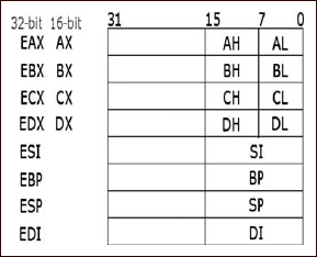
In IA-32 there are eight 32-bit general purpose registers, six 16-bit segment registers, one 32-bit instruction pointer register, one 32-bit status register, five control registers, three memory management registers, eight debug registers, and so on. In most cases you will only be dealing with the general purpose registers, the instruction pointer, the segment registers and the status register. If you’re dealing with OS drivers or similar, you’re more likely to encounter the other registers. Here we’re going to cover the general purpose registers, the instruction pointer, the status register and the segment registers. As for the others, it’s probably good enough just to know they exist, although naturally the interested reader is encouraged to consult the Intel documentation for further details.

The eight 32-bit general purpose registers are as follows: EAX, EBX, ECX, EDX, ESI, EDI, EBP and ESP. These registers can mostly be used as one sees fit, with a few notable exceptions. For instance, many instructions assign specific registers to certain arguments (or operands). As a specific example, many of the string instructions use ECX as a counter, ESI as a source pointer and EDI as a destination pointer. Furthermore, some of these instructions imply the use of a given segment as a base address in certain memory models (both are covered shortly). Finally, other registers are implied during certain operations. For instance, the EBP and ESP registers are used in many stack operations and their values containing an address that is not mapped into the current process’s address space will often result in the application crashing. The IA-32 architecture is almost entirely backwards compatible to the 8086 processor and this is reflected in their registers; all of the general purpose registers can be accessed in a manner yielding the register’s full 32-bit contents or its lower 16 bits, and the EAX, EBX, ECX and EDX registers can have their high-order and lower-order 8 bits accessed as well. This is accomplished by using the names reflected in Figure 2.1. For instance, to access the low-order 8 bits of the EAX register, you would replace EAX in your instruction with AL; to access the lower 16 bits of the EBP register you would replace EBP with BP; and to access the second set of 8 bits in the low-order 16 bits of the EDX register, you would replace EDX with DH. In addition to the general purpose registers, we also have the instruction pointer, EIP. The EIP register points to the next instruction to be executed by the processor and by implication the goal of almost any application-based attack is to control this register. Unlike the general purpose registers, however, it cannot be directly modified. This is to say that you cannot execute an instruction to move a value into the register, but rather you would have to perform a set of operations that indirectly modify its value, such as a push onto the stack segment followed by a ret instruction. Don’t worry if that last sentence was a bit outlandish and you didn’t quite understand it yet; both of the instructions referenced and the stack segment will be covered in detail later on in the chapter. Just for now, know that you cannot directly modify the value of the instruction pointer.

Figure 2.1. General Purpose Registers

In addition to the EIP register and the general purpose register, we have six 16-bit segment registers: code segment (CS), data segment (DS), stack segment (SS), extra segment (ES), and FS and GS, which are extra general purpose segments. The segment registers contain a pointer to what are called segment selectors and these are often used as a base address from which to take an offset; for instance, consider the following instruction:

mov DS:[eax], ebx

In this instruction, the contents of the EBX register are copied into an offset into the data segment specified by EAX. Think of this as saying “the address of DS plus the contents of EAX.” Segment selectors are a 16-bit identifier for segments, which is to say the segment selector does not point directly to the segment, but rather to a segment descriptor that defines the segment. So, segment registers point to segment selectors, which are used to identify one of the 8192 possible segment descriptors that identify segments. Confused yet?

The segment selectors are relatively simple structures. The bits at 3 through 15 are used as an index into one of the descriptor tables (one of the three memory management registers), bit 2 specifies which descriptor table exactly, and finally the low-order two bits specify a requested privilege level (ranging 0 through 3—privilege levels are discussed later in the chapter). Segment descriptors, while interesting and fairly important to OS design, are again not covered in order to ensure only information relevant to your general purposes is contained in this chapter. As always, the interested reader is encouraged to refer back to the Intel developer manuals. Finally, in the description of the various relevant registers, we have the EFLAGS register, which contains groups of various flags that indicate the states of previous instructions, status, and things such as the current privilege level and whether interrupts are enabled or not. In the current context of things, the EFLAGS register can’t really make sense until we have a better grasp of some of the instructions that make use of it, and as such a thorough description of it is reserved until later in the chapter.

Now that we’ve described both constant and register operands, it’s time to discuss memory operands. Memory operands can be a little bit tricky, although at this stage in the game their description is pretty limited. A memory operand is by and large what a high-level language programmer thinks of as a variable. That is to say that when you declare a variable in a language like C or C++, it’s by and large going to exist in memory and thus it will often be a memory operand. These are typically accessed through a pointer, which when dereferenced will either result in the value being loaded into a register or accessed directly from memory. The concept itself is pretty simple, but truly understanding what is going on requires a bit deeper knowledge of how memory is addressed, which in turn depends on the memory model, mode of operation and privilege level being used. This provides an excellent lead into the next few paragraphs, which cover mode of operation.

In IA-32, there are three basic operating modes and one pseudomode of operation. They are protected mode, real-address mode and system management mode, with the pseudomode being a subset of protected mode called virtual-8086 mode. In the interest of brevity, only protected mode will be discussed in detail. The biggest difference between the various operating modes is that they modify what instructions and architectural features are present. For instance, RM (also often called real mode) is meant for backwards compatibility, and in RM only the real-address mode memory model is supported. The main thing of importance to note here (unless you’re reversing old DOS applications or similar), is that when you reset or first power up an IA-32 PC, it is in real mode natively. System management mode (SMM), which has been in the Intel architecture since the 80386 and is used in implementing things such as power management and system hardware control, is also used. It basically stops all other operations and switches to a new address space. Generally speaking, however, almost everything you encounter and use will be in protected mode.

Protected mode represented a huge advancement in the Intel architecture when it was introduced on the 80286 processor and further refined on the 80386 processor. One key issue was that previous versions of the processor supported only one mode of operation and had no inherent hardware-enforced protections on instructions and memory. This not only allowed rogue operators to do anything they wanted, but it also allowed for a faulty application to crash the entire system, so it was an issue of both reliability and security. Another issue with prior processor versions was the 640 KB barrier; this is something else that PM overcame. Furthermore, there were other advances, such as hardware-supported multitasking and modifications in how interrupts were handled. Indeed, the 286 and 386 represented significant advances in personal computing.

In the earlier days, such as with the 8086/80186 processor, or today when a modern processor is in real-address mode, the segment register represents the high-order 16 bits of a linear address, whereas in protected mode the selector is an index into one of the descriptor tables. Furthermore, as previously mentioned, with earlier CPUs there was no protection of memory or limit to instructions; in protected mode, there are four privilege levels called rings. These rings are given numbers for identification ranging from 0 to 3, with the lowest number being the highest privilege level. Ring-0 is typically used for the operating system, whereas ring-3 is where applications typically run. This protects the OS’s data structures and objects from modification by a broken or rogue application and restricts instructions that those applications can run (what good would the levels be if the ring-3 application could just switch its privilege level?). In IA-32 there are three places to find privilege level: in the low-order 2 bits of the CS register there is the Current Privilege Level (CPL), in the low-order 2 bits of a segment descriptor is the Descriptor Privilege Level (DPL), and in the low-order 2 bits of a segment selector is the Requestor’s Privilege Level (RPL). The CPL is the privilege level of the currently executing code, the DPL is the privilege level of the given descriptor, and, somewhat obviously, the RPL should be the privilege level of the code that created that segment.

The privilege levels restrict access to more trusted components of the system’s data; for instance, a ring-3 application cannot access the data of a ring-2 component. However, the ring-2 component can access the data of a ring-3 component. This is why you can’t arbitrarily read data from the Windows or Linux kernel but it can read yours. Another function of this privilege-level separation is that it performs checks on execution transfer control. A request to change execution from the current segment to another causes a check to be performed, ensuring that the CPL is the same as the segment’s DPL. Indirect transfers of execution occur via things such as call gates (which are briefly covered later). Finally, privilege levels restrict access to certain instructions that would fundamentally change the environment of the OS or operations that are typically reserved for the OS (such as reading or writing from a serial port).

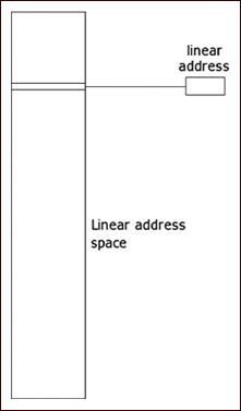
Moving on from protected mode, we have the three different memory models: flat, segmented and real-address. Real-address mode is used at boot time and is kept around for backwards compatibility; however, it is quite likely you will never (or very rarely) encounter it and thus it’s not discussed in this chapter. The flat memory model is about what you’d expect it to be from its name: it’s flat (see Figure 2.2)! This means basically that the systems memory appears as a single contiguous address space, ranging from address 0 to 4294967296 in most instances. This address space is referred to as the linear address space, with any individual address being known as a linear address. In this memory model, all of the segments—code, stack, data, and so forth—fall within the same address space. Despite what you may be inclined to first think, this is the memory model used by nearly all modern OSes and chances are your computer’s OS at home employs it. This seems like it would lead to disaster and unreliability; however, it is almost universally used with paging, which we’ll discuss shortly.

Figure 2.2. Flat Memory Model

The flat memory model in protected mode differs only in that the segment limits are set to ensure that only the range of addresses that actually exist can be accessed. This differs from other modes, where the entire address space is used and there may be gaps of unusable memory in the address space.

The next memory model is the segmented memory model. It was used in earlier operating systems and has seen somewhat of a comeback, as in some arenas it implies an increase in speed (due to the ability to skip relocation operations) and security. Nonetheless, this memory model is still pretty rare and whether it makes a full comeback is yet to be seen, although it’s a bit unlikely. It’s described here because, if you do much reverse engineering or exploit development under Linux, your likelihood of encountering it goes up considerably.

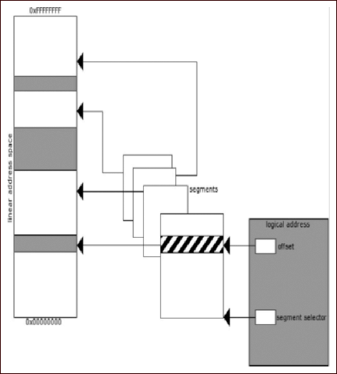
In a segmented memory model, the systems memory is split up into subsections called segments. (See Figure 2.3.) These segments are kept independent and isolated from each other. To compare the segmented and flat memory models for a moment, what is really different between them is their representation to an OS or application. In both instances, the data is still stored in a linear fashion; however, the view of that data changes. With segmented memory, instead of issuing a linear address to access memory, a logical address (also known as a far pointer) is used. A logical address is the combination of a base, which is stored in a segment selector, and an offset. These two correspond to an address in that segment, which in turn maps to the linear address space. What this accomplishes is a higher degree of segmentation that is enforced by the processor, ensuring that one process does not run into another process (whereas in a flat memory model the same result is hopefully accomplished by the OS). Thus, the base address plus the offset equals a linear address in the processor’s address space. Furthermore, a multiple segment model can be used that retains the same traits as a single segmented model, except each application is given its own set of segments and segment descriptors. At the present time, the author cannot think of an OS that employs this, so a further description of how it works is moot.

Figure 2.3. Segmented Memory Model

As a result of modern OSes often using larger address space than physical memory can accommodate, some form of addressing all of the necessary data without requiring that it be stored in physical memory is required. The answer comes in the form of paging and virtual memory, one of the fundamental tenets of modern computing that is often misunderstood by people with a more operations-oriented background. It’s not uncommon to encounter people who understand that a given application can be given 4 GB of memory but who don’t really comprehend how that could possibly work, given that they only have 1 or 2 GB of physical memory.

In short, paging takes advantage of the fact that only the currently necessary data needs to be stored in physical memory at any given moment; it stores what data it needs in physical memory and stores the rest on disk drive. The process of loading memory with data from disk, or writing data to disk, is known as swapping data, and this is why Windows boxes typically have swap files and Linux boxes usually have swap partitions. When paging is not enabled, a linear address (whether it be formed from a far pointer or not) has a one-to-one mapping with a physical address and no translation between it and the issued address occurs. However, when paging is enabled, all pointers used by an application are virtual addresses. (This is why two applications in a protected mode flat memory model using paging accessing the exact same address don’t trample each other.) These virtual addresses do not have a one-to-one mapping with a physical memory address.

When paging is employed, the processor splits the physical memory into 4 KB, 2 MB or 4 MB pages. When an address is turned into a linear address and then through the paging mechanism it is looked up, if the address does not currently exist in physical memory then a page-fault exception occurs, instructing the OS to load the given page into memory and then performing the instruction that generated the fault again.

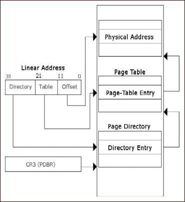
The process of translating a virtual address to a physical address varies depending on the page size being used, but the basic concept is the same either way. A linear address is divided into either two or three sections. First the Page Directory Base Register (PDBR) or Control Register 3 (CR3) is used to locate a Page Directory. Following this, bits 22 through 31 in the linear address are used as an offset into the Page Directory which identifies a given Page Table to use. (See Figure 2.4.) Once the Page Table has been located, the bits 12 through 21 are used to locate a Page Table Entry (PTE), which identifies the page of memory to be used. Finally bits 0 through 11 of the linear address are used as an offset into the page to locate the data requested. When using other side pages, the process is nearly identical except that one layer of indirection is omitted; the directory entry points directly to the page and the page table and PTEs are completely omitted. The contents of Page Directory Entries (PDEs) and PTEs are not important for our purposes. If they become important to you at some point or if you’re just curious, please refer to the processor’s documentation.

Figure 2.4. 4 KB Address Translation

Now that we have a decent understanding of instructions and operands, memory models, operating modes and so on, we can move on. Most of the terms employed later on in this chapter and throughout the book have now been defined, so you can refer back to this section should you feel like you don’t understand something as you work through the book.

In the previous section we talked some about segments, segment registers, segment descriptors and segment selectors, but we really didn’t delve into the data that they contain. Understanding these various sections is fairly important to understanding the layout of a binary executable. In this section we will discuss these concepts as much as possible, although in some areas, such as with the heap, it’s not really possible to jump into the depths of how it works exactly without a fairly in-depth analysis of a particular implementation; in those instances a generic high-level overview is provided and the understanding of the most minute details is left as an exercise for the reader.

Earlier we discussed the segment registers, in particular the CS, DS and SS segment registers, but we didn’t tell you what the code, data and stack segments were. In traditional design, an application has a few different basic sections (and a lot of implementation-specific ones). The basic ones employed are the code segment (or text segment or simply .text), the data segment (often simply .data), the block started by symbol (BSS/.bss) segment, the stack segment and the heap segment. As an example, the following C code will help demonstrate the differences between the various sections:

unsigned int variable_zero;
unsigned int variable_one = 0x1234;
int
main(void)
{
       void * variable_two = malloc(0x1234);
       [...]
}

In this code example, we have three variables defined and one function. The first variable, appropriately named variable_zero, is a variable of global scope that is uninitialized. In this instance, the C compiler will allocate space in the binary and fill it with zeros. The section of the binary it will exist in is the BSS section. The variable named variable_one is another globally scoped variable. However, in this instance it is initialized to the value 0×1234. In this instance, the compiler will preallocate the space for the variable in the binary and store the value in the data segment. Following this, we have the function main. Main obviously is a function, and thus is in the code segment. After main we find the variable called variable_two, which gives us an interesting predicament: we have a pointer whose scope is inside of main and the memory that it points to. The pointer itself is local to the function, is dynamically allocated and exists on the stack segment, giving it a lifetime of the function it exists in, whereas the pointer returned by malloc( ) exists on the heap, is dynamically allocated and has a global scope and a “use-until-free( )” life expectancy. There are also often other sections; for instance, in programs compiled by the GNU compiler collection (GCC) a constant string that is declared in the source file will often end up in a section named .rodata, for read-only data, or in the code segment.

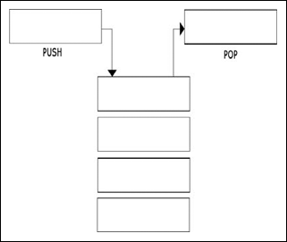
The stack is one of the more important sections to understand, as it plays a vital role in the routine operations of an application. Those with a formal computer science background will no doubt know what a stack is and how it works. A stack is a simple data structure that basically stacks data on top of each other and has elements added and removed in a last-in first-out (LIFO) manner. When you add an item to the stack, you push it onto a stack, and when you remove an item from a stack, you pop it off the stack. (See Figure 2.5.) The stack is important for two basic reasons on most computing platforms. The first is that all automatic or local variables are stored on it; that is, when a function is called, any local variables it has declared that are not static or similar have their space allocated on the stack. This is usually realized by adding or subtracting a number from the current stack pointer. The stack pointer is the ESP register, and it normally points to the top of the stack segment, or rather SS:ESP points to the top of the stack segment. The top of the stack is the lowest currently in use address of the stack—the lowest because the stack grows down on IA-32. The bottom of the stack is usually bounded, not by the absolute bottom, but the bottom of the current stack frame and is pointed to by the EBP register.

Figure 2.5. A Stack

A stack frame is the current view into the stack relevant to the currently executing function; when the processor enters a new procedure, a few steps occur known as the procedure prologue. (See Figure 2.6.) The procedure prologue is as follows: the routine first pushes the address of the next instruction in the calling frame onto the stack; next the current base (EBP) of the stack is saved onto the stack; the ESP register is then copied into the EBP register; and finally the ESP register is decremented to allocate space for variables in that function. When the function is called, the arguments to the function are pushed onto the stack in reverse order (or the last one is pushed first). The assembly generated for the prologue is as follows:

push ebp
mov ebp, esp
sub esp, 0x1234

Figure 2.6. Stack Frame

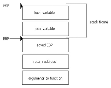
What we see here is strangely missing the saving of the return address, or the address we will continue execution at in the calling routine. For instance, given the following C code:

A();
B();

when inside of the function A( ) the return address would be the address of the instruction B( ). It’s a little tricky to understand at first, especially because you don’t ever see the instruction that saves the address onto the stack, but rather it is implied by using the call instruction, which is discussed a little later on in the chapter. In addition to the procedure prologue, there is also the procedure epilogue. The procedure epilogue basically undoes everything that the prologue did. This includes incrementing the stack pointer to deallocate any local variables, and then calling the leave and ret instructions, which remove the saved frame pointer and return address and return execution flow to the calling function. So, to summarize the points on the stack:

The heap is another important data structure, but not because any features of the processor depend on it, but rather because of the large amount of use it receives. The heap is simply a section of memory that is used for dynamically allocated variables that need to exist outside of the current stack frame; as a result of trait, most of the objects and indeed large amounts of the data an application uses will be on the heap. The heap is usually either the result of a random mapping or in more classic examples it was a dynamic extension of the data segment (although DS rarely if ever points to the heap). In that sense, the processor is by and large ignorant and the details are hidden away from the processor. Furthermore, the OS knows very little about the user-land heap; when requested, it simply gives the application more memory if possible and fails otherwise. It is typically the libc or similar that provides the heap operations and thus defines its semantics.

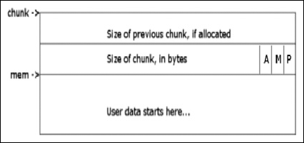
The heap, typically upon initialization, will request a fairly large section of memory from the OS, and will hand out smaller chunks of memory based upon requests from the application. These chunks will typically have inline metadata indicating the chunk’s size and other elements, such as the size of the previous block of memory.

The blocks of allocated memory are navigated by taking the pointer to a given chunk and adding its size to it to find the next chunk, or by subtracting the previous size from the beginning of the chunk to find the previous one. For instance, in Figure 2.7 you will find an example of an allocated chunk as represented in Glibc. In this instance the pointer labeled mem indicates that start of data returned to the API user by malloc( ) or similar, whereas the pointer labeled chunk marks the beginning of the actual chunk. There we find that there is metadata including the size of the previous chunk and the size of the current chunk, along with flags indicating various status conditions. This chunk, while mostly used by Linux, is generically similar to chunks used by most operating systems and dynamic memory allocator implementation (with, of course, some key differences). Since initially obtaining that large chunk of memory from the OS or extending the size of the data segment are fairly expensive operations, a cache of sorts is usually maintained. This cache usually comes in the form of a linked list of pointers to previously free( )’d chunks of memory. This list is typically fairly complex, with the blocks of memory being coalesced into adjacent free blocks of memory to reduce fragmentation, and with various lists sorted by size or some other characteristic to allow the most efficient means possible of locating a candidate block of memory whenever an allocation request occurs.

Figure 2.7. Glibc Allocated Chunk

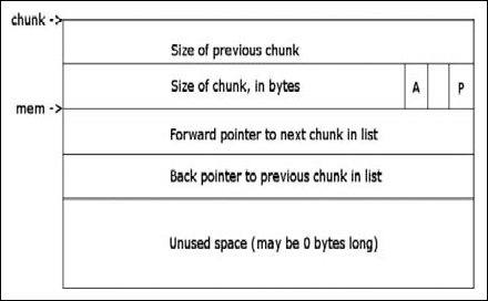
To use a similar example to the previous one, in Figure 2.8 you will see the representation of a free block of memory as represented by Glibc. In this instance, the pointer labeled mem indicates where the pointer returned to the API user used to be, and the one labeled chunk points to the beginning of the physical data structure used. The biggest difference is that in what used to be user data, there are now two pointers stored pointing to the next free block of memory in the linked list and the previous block of memory in the linked list. This of course implies that, unlike allocated chunks which are navigated by size, a free block of memory is navigated directly by linked list. The specific details of the structure listed are, again, specific to Glibc; however, the concept itself is generic enough to apply to most implementations. Thus, as allocation and free requests come in and out, which happens quite frequently throughout the lifetime of your average application, chunks are taken away from the original chunk of memory obtained from the OS and returned to free lists, and then if possible further allocation requests make use of these blocks of memory on the free list, and so on until either all memory is in use, or the application terminates.

Figure 2.8. Glibc Free Chunk

In the previous section, we’ve discussed the most common sections of a binary executables layout, including some of their functions, and took a more in-depth tour of the stack segment and the heap segment and talked about how they worked to some degree. This should be enough to provide a base to continue building your understanding. Of course, the interested reader is encouraged to refer to other works more specifically targeted at questions they may have on these subjects.

In the prior sections, we talked briefly about instructions and operands, but focused more on the architectural design of IA-32 and then delved into some common layouts for binary executable memory and their purposes and uses. In this section the intention is to provide you with a reference for some of the more commonly used instructions and talk to you some about their uses and operands. If by now you’ve already read the Intel developer manuals, then this section is likely to be redundant and you may wish to skip directly to the next chapter. In this section the terminology shown in Table 2.1 will be used.

The first instruction we are going to cover is the mov instruction, which is a very basic instruction that copies one operand to the other. It can take the forms and allows the operands shown in Table 2.2.

The mov instruction copies the source operand to the destination operands and can only be used to move certain types of operands; for instance, it cannot be used to set the Code segment, and it cannot be used to modify the EIP register. If a destination operand is of type Sreg, then it must point to a valid segment selector. The next instructions introduced will be the various bitwise operations such as and and exclusive or.

The and instruction is another fairly simple instruction. It performs a bitwise AND on the destination operand with the source operand, storing the result in the destination operand. It supports the operands shown in Table 2.3. A bitwise AND compares the binary representation of the two operands, and sets the output bit to 1 if both bits compared are turned on; otherwise the result is a turned-off bit.

The next instruction referenced is the not instruction, another fairly simple but commonly used instruction; it performs a bitwise NOT operation on a single operand and allows the operands shown in Table 2.4. This simply sets each 1 to 0 and vice versa in its operand.

Chugging forward, we have the or instruction, which performs a bitwise OR on its arguments and takes the arguments shown in Table 2.5. A bitwise OR is, again, a fairly simple operation that’s used often. It compares the two operands bit by bit and sets the corresponding output bit to zero only if both compared bits are set to zero.

Next in the line-up we have the exclusive-or instruction, or xor. It performs a bitwise exclusive-or (XOR) on its operands and takes the operands shown in Table 2.6. The xor instruction compares the source and the destination operands and stores the output in the destination operand. Each output bit is 1 if the two compared bits are different; otherwise the output bit is 0.

The test instruction is commonly used to determine a specific condition and then modify control flow based on the results (see Table 2.7). The test instruction performs a bitwise AND of the first and second operands, and then sets flags in the EFLAGS register accordingly. Following this, the result is then discarded.

The cmp instruction compares two operands; this comparison is performed by subtracting the source operands from the destination operands and setting flags in the EFLAGs register accordingly (see Table 2.8). It is often used in a manner similar to the test instruction and is used to compare values like user input and return values from routines. If an immediate value is used as an operand, it is sign-extended to match the size of the other operand.

The load effective address instruction, or lea, calculates the address as specified by the source operand and stores it in the destination operand (see Table 2.9). It is also used as a method for doing arithmetic between multiple registers without modifying the source operands.

The jmp instruction transfers execution control to its operand. This instruction can execute four different types of jumps: a near jump, a short jump, a far jump and a task switch (see Table 2.10). A near jump is a jump that occurs within the current code segment. A short jump is a jump to an address within −128 to 127 from the current address. A far jump can take control to any segment in the address space providing it is of the same privilege level as the current code segment. Finally, a task switch jump is a jump to an instruction in a different task.

The jcc instructions are not one particular instruction, but rather a series of conditional jumps. The conditions vary with the instruction used, but they’re typically used in collaboration with the test and cmp instructions. Table 2.11 shows destination operands for jcc instructions. In Table 2.12 you will find a list of conditional jumps and the flags that they check to determine whether a condition is true or not. Don’t worry about the flags just yet; the description of the EFLAGS register will come just after the instructions.

So, as you can see in Table 2.12, there are quite a few conditional jump registers, and all of them depend on the various states of the EFLAGS register, which we haven’t really described yet, but will do now. The EFLAGS register is a 32-bit register that contains a group of status and system flags, and a control flag. Each flag is represented by a single bit in this register, and moving from bit 0 to 31 we have the following flags:

Bits 22 through 31 are currently reserved.

The call instruction is somewhat akin to a more official jump; it sets up the stack as previously described in a manner that will allow the processor to resume execution in the calling function when the executed function finishes. (See Table 2.13.)

The ret instruction is the inverse of the call instruction. It takes the metadata stored on the stack, pops it off and returns to that address (see Table 2.14). The optional immediate operand specifies how many bytes to pop off of the stack after performing the return.

As you can see, there are already a lot of instructions to be familiar with, and most of them take many different operands, which in turn results in many different forms of the same instruction (and thus different opcodes). This is hardly a complete instruction reference—in fact, it barely scratches the surface. However, we wanted to touch base on some of the more commonly used instructions and at least familiarize you with them. Readers are strongly encouraged to consult the Intel developer manuals, specifically 3A and 3B, if they are not already familiar with the instruction set.

So now you’re at least familiar with assembly and the Intel architecture. You know how the memory models and operating modes work to some degree and have a decent general base of comprehension to build on. However, you might find yourself thinking, “Yes, I understand some assembly now, but what is reverse engineering?”. Well, reverse engineering is a broad term and means different things to different people. In general, the answer is that it’s the process of taking an application that is in a form not meant for human readability or analysis and working backwards towards the beginning. Some people do this in order to regain lost source code, others do it to duplicate proprietary products, some reverse malicious applications to know what they do, and finally others reverse engineer software to find bugs and vulnerabilities in it.

To be brief, and for the purposes of this book, reverse engineering is taking a binary file that is meant to be read by the computer and using the opcodes to generate assembly, and then reading that assembly to help accomplish whatever goals you may have. In this sense, it can be said that, to the reverse engineer, there is no such thing as closed source software. The processor sees every instruction, and so does the reverse engineer.