Table of Contents for
Graph Algorithms
 Graph Algorithms
Published by
O'Reilly Media, Inc., 2019
Graph Algorithms
Published by
O'Reilly Media, Inc., 2019
- Cover
- nav
- Graph Algorithms
- Graph Algorithms
- Preface
- 1. Introduction
- 2. Graph Theory and Concepts
- 3. Graph Platforms and Processing
- 4. Pathfinding and Graph Search Algorithms
- 5. Centrality Algorithms
- 6. Community Detection Algorithms
- 7. Graph Algorithms in Practice
- 8. Using Graph Algorithms to Enhance Machine Learning
- About the Authors
Chapter 6. Community Detection Algorithms
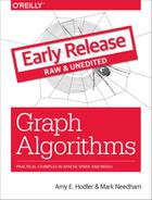
Community formation is common in complex networks for evaluating group behavior and emergent phenomena. The general principle in identifying communities is that a community will have more relationships within the group than with nodes outside their group. Identifying these related sets reveals clusters of nodes, isolated groups, and network structure. This information helps infer similar behavior or preferences of peer groups, estimate resiliency, find nested relationships, and prepare data for other analysis. Commonly community detection algorithms are also used to produce network visualization for general inspection.
We’ll provide detail on the most representative community detection algorithms:
-
Triangle Count and Clustering Coefficient for overall relationship density
-
Strongly Connected Components and Connected Components for finding connected clusters
-
Label Propagation for quickly inferring groups based on node labels
-
Louvain Modularity for looking at grouping quality and hierarchies
We’ll explain how the algorithms work and show examples in Apache Spark and Neo4j. In cases where an algorithm is only available in one platform, we’ll provide just one example. We use weighted relationships for these algorithms because they’re typically used to capture the significance of different relationships.
Figure 6-1 illustrates and overview of differences between the community detection algorithms covered and Table 6-1 provides a quick reference to what each algorithm calculates with example uses.
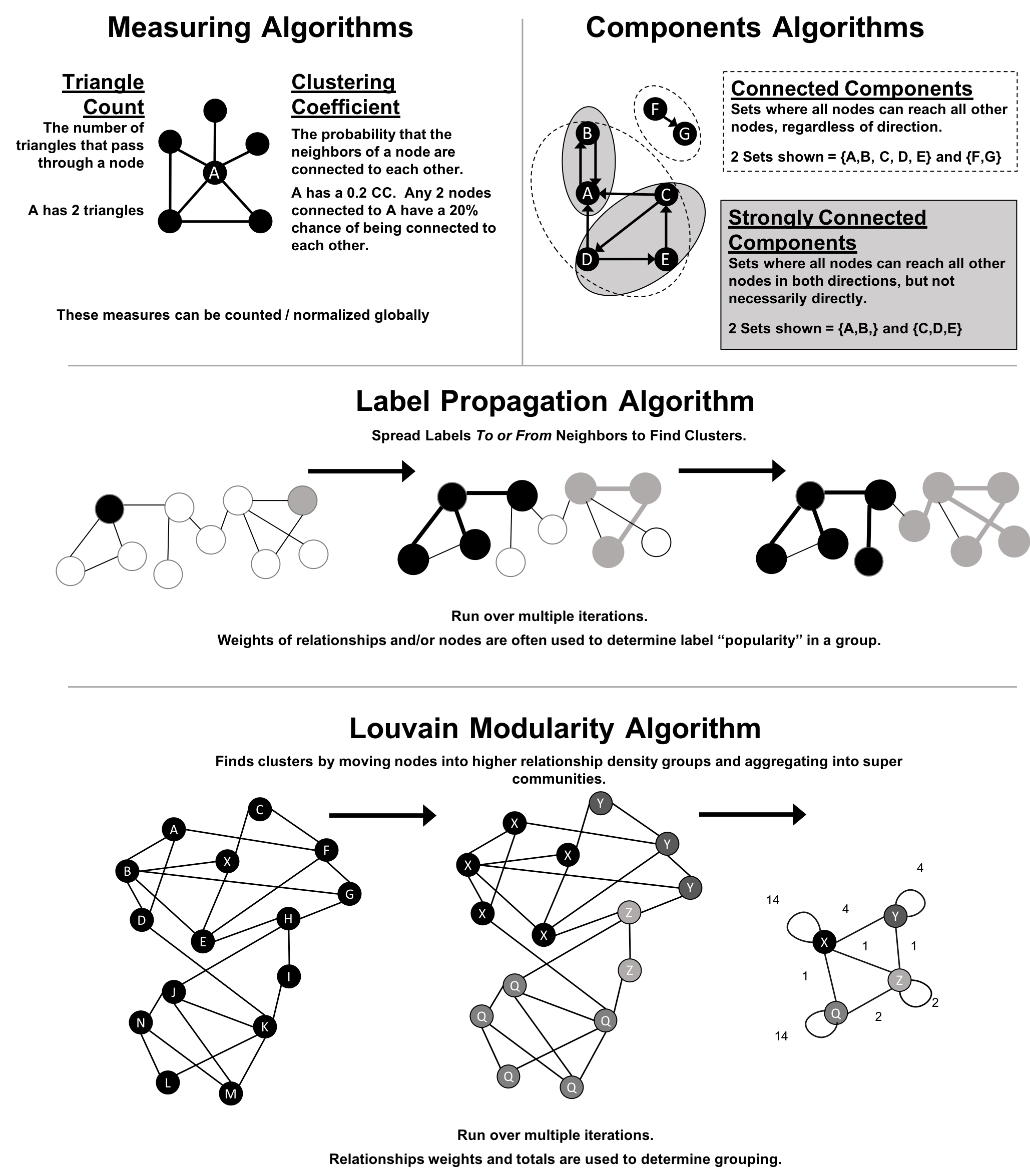
Figure 6-1. Representative Community Detection Algorithms
Note
We use the terms “set,” “partition,” “cluster,” “group,” and “community” interchangeably. These terms are different ways to indicate that similar nodes can be grouped. Community Detection algorithms are also called clustering and partitioning algorithms. In each section, we use the terms that are most prominent in the literature for a particular algorithm.
| Algorithm Type | What It Does | Example Uses | Spark Example | Neo4j Example |
|---|---|---|---|---|
Measures how many nodes form triangles and the degree to which nodes tend to cluster together. |
Estimate group stability and whether the network might exhibit “small-world” behaviors seen in graphs with tightly knit clusters. |
Yes |
Yes |
|
Finds groups where each node is reachable from every other node in that same group following the direction of relationships. |
Make product recommendations based on group affiliation or similar items. |
Yes |
Yes |
|
Finds groups where each node is reachable from every other node in that same group, regardless of the direction of relationships. |
Perform fast grouping for other algorithms and identify islands. |
Yes |
Yes |
|
Infers clusters by spreading labels based on neighborhood majorities. |
Understand consensus in social communities or find dangerous combinations of possible co-prescribed drugs. |
Yes |
Yes |
|
Maximizes the presumed accuracy of groupings by comparing relationship weights and densities to a defined estimate or average. |
In fraud analysis, evaluate whether a group has just a few discrete bad behaviors or is acting as a fraud ring. |
No |
Yes |
First, we’ll describe the data for our examples and walk through importing data into Apache Spark and Neo4j. You’ll find each algorithm covered in the order listed in Table 6-1. Each algorithm has a short description and advice on when to use it. Most sections also include guidance on when to use any related algorithms. We demonstrate example code using a sample data at the end of each section.
Note
When using community detection algorithms, be conscious of the density of the relationships.
If the graph is very dense, we may end up with all nodes congregating in one or just a few clusters. You can counteract this by filtering by degree, relationship-weights, or similarity metrics.
On the other hand, if it’s too sparse with few connected nodes, then we may end up with each node in its own cluster. In this case, try to incorporate additional relationship types that carry more relevant information.
Example Graph Data: The Software Dependency Graph
Dependency graphs are particularly well suited for demonstrating the sometimes subtle differences between community detection algorithms because they tend to be densely connected and hierarchical. The examples in this chapter are run against a graph containing dependencies between Python libraries, although dependency graphs are used in various fields from software to energy grids. This kind of software dependency graph is used by developers to keep track of transitive interdependencies and conflicts in software projects. You can download the nodes1 and relationships2 files from the book’s GitHub repository3.
sw-nodes.csv
| id |
|---|
six |
pandas |
numpy |
python-dateutil |
pytz |
pyspark |
matplotlib |
spacy |
py4j |
jupyter |
jpy-console |
nbconvert |
ipykernel |
jpy-client |
jpy-core |
sw-relationships.csv
| src | dst | relationship |
|---|---|---|
pandas |
numpy |
DEPENDS_ON |
pandas |
pytz |
DEPENDS_ON |
pandas |
python-dateutil |
DEPENDS_ON |
python-dateutil |
six |
DEPENDS_ON |
pyspark |
py4j |
DEPENDS_ON |
matplotlib |
numpy |
DEPENDS_ON |
matplotlib |
python-dateutil |
DEPENDS_ON |
matplotlib |
six |
DEPENDS_ON |
matplotlib |
pytz |
DEPENDS_ON |
spacy |
six |
DEPENDS_ON |
spacy |
numpy |
DEPENDS_ON |
jupyter |
nbconvert |
DEPENDS_ON |
jupyter |
ipykernel |
DEPENDS_ON |
jupyter |
jpy-console |
DEPENDS_ON |
jpy-console |
jpy-client |
DEPENDS_ON |
jpy-console |
ipykernel |
DEPENDS_ON |
jpy-client |
jpy-core |
DEPENDS_ON |
nbconvert |
jpy-core |
DEPENDS_ON |
Figure 6-2 shows the graph that we want to construct. Just by looking at this graph we can clearly see that there are 3 clusters of libraries. We can use visualizations as a tool to help validate the clusters derived by community detection algorithms.
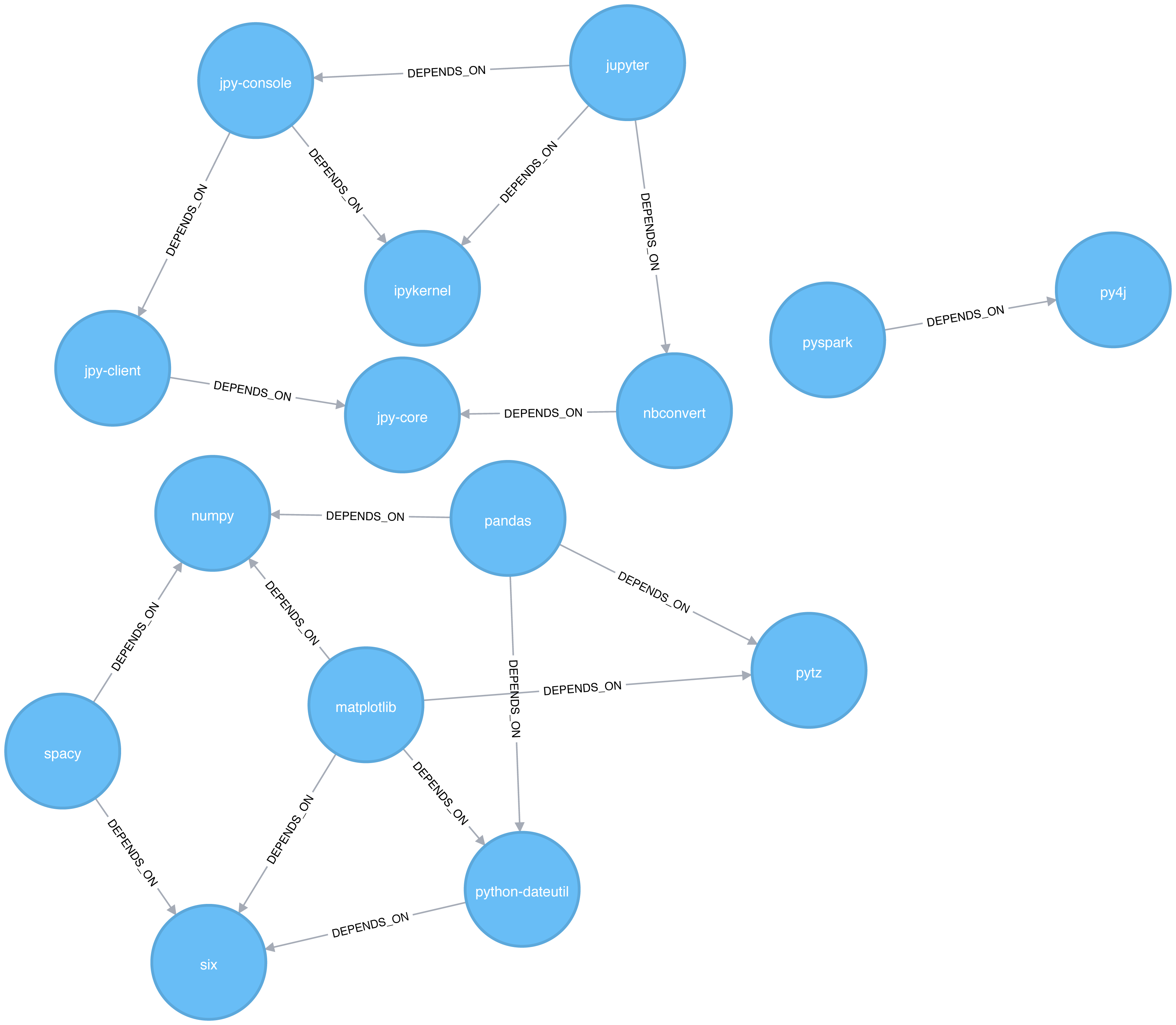
Figure 6-2. Graph model
Let’s create graphs in Apache Spark and Neo4j from the example CSV files.
Importing the data into Apache Spark
We’ll first import the packages we need from Apache Spark and the GraphFrames package.
fromgraphframesimport*
The following function creates a GraphFrame from the example CSV files:
defcreate_software_graph():nodes=spark.read.csv("data/sw-nodes.csv",header=True)relationships=spark.read.csv("data/sw-relationships.csv",header=True)returnGraphFrame(nodes,relationships)
Now let’s call that function:
g=create_software_graph()
Importing the data into Neo4j
Next we’ll do the same for Neo4j. The following query imports nodes:
WITH"https://github.com/neo4j-graph-analytics/book/raw/master/data/sw-nodes.csv"ASuriLOAD CSVWITHHEADERS FROM uriASrowMERGE (:Library {id: row.id})
And then the relationships:
WITH"https://github.com/neo4j-graph-analytics/book/raw/master/data/sw-relationships.csv"ASuriLOAD CSVWITHHEADERS FROM uriASrowMATCH(source:Library {id: row.src})MATCH(destination:Library {id: row.dst})MERGE (source)-[:DEPENDS_ON]->(destination)
Now that we’ve got our graphs loaded it’s onto the algorithms!
Triangle Count and Clustering Coefficient
Triangle Count and Clustering Coefficient algorithms are presented together because they are so often used together. Triangle Count determines the number of triangles passing through each node in the graph. A triangle is a set of three nodes, where each node has a relationship to all other nodes. Triangle Count can also be run globally for evaluating our overall data set.
Note
Networks with a high number of triangles are more likely to exhibit small-world structures and behaviors.
The goal of the Clustering Coefficient algorithm is to measure how tightly a group is clustered compared to how tightly it could be clustered. The algorithm uses Triangle count in its calucluations which provides a ratio of existing triangles to possible relationships. A maximun value of 1 indicates a clique where every node is connected to every other node.
There are two types of clustering coefficients:
Local clustering coefficient
The local clustering coefficient of a node is the likelihood that its neighbors are also connected. The computation of this score involves triangle counting.
The clustering coefficient of a node can be found by multiplying the number of triangles passing through a node by two and then diving that by the maximum number of relationships in the group, which is always the degree of that node, minus one. Examples of different triangles and clustering coefficients for a node with 5 relationships is protrayed in Figure 6-3.
Figure 6-3. Triangle Count and Clustering Coefficient for u
The clustering coefficient for a node uses the formula:
where:
-
uis a node -
R(u)is the number of relationships through the neighbors ofu(this can be obtained by using the number of triangles passing throughu.) -
k(u)is the degree ofu
Global clustering coefficient
The global clustering coefficient is the normalized sum of the local clustering coefficients.
Clustering coefficients give us an effective means to find obvious groups like cliques, where every node has a relationship with all other nodes, but also specify thresholds to set the levels, say where nodes are 40% connected.
When Should I Use Triangle Count and Clustering Coefficient?
Use Triangle Count when you need to determine the stability of a group or as part of calculating other network measures such as the clustering coefficient. Triangle counting gained popularity in social network analysis, where it is used to detect communities.
Clustering Coefficient can provide the probability that randomly chosen nodes will be connected. You can also use it to quickly evaluate the cohesiveness of a specific group or your overall network. Together these algorithms are used to estimate resiliency and look for network structures.
Example use cases include:
-
Identifying features for classifying a given website as spam content. This is described in Efficient Semi-streaming Algorithms for Local Triangle Counting in Massive Graphs 4.
-
Investigating the community structure of Facebook’s social graph, where researchers found dense neighborhoods of users in an otherwise sparse global graph. Find this study in The Anatomy of the Facebook Social Graph 5.
-
Exploring the thematic structure of the Web and detecting communities of pages with a common topics based on the reciprocal links between them. For more information, see Curvature of co-links uncovers hidden thematic layers in the World Wide Web 6.
Triangle Count with Apache Spark
Now we’re ready to execute the Triangle Count algorithm. We write the following code to do this:
result=g.triangleCount()result.sort("count",ascending=False)\.filter('count > 0')\.show()
If we run that code in pyspark we’ll see this output:
| count | id |
|---|---|
1 |
jupyter |
1 |
python-dateutil |
1 |
six |
1 |
ipykernel |
1 |
matplotlib |
1 |
jpy-console |
A triangle in this graph would indicate that two of a node’s neighbors are also neighbors. 6 of our libraries participate in such triangles.
What if we want to know which nodes are in those triangles? That’s where a triangle stream comes in.
Triangles with Neo4j
Getting a stream of the triangles isn’t available using Apache Spark, but we can return it using Neo4j:
CALL algo.triangle.stream("Library","DEPENDS_ON")YIELD nodeA, nodeB, nodeCRETURNalgo.getNodeById(nodeA).idASnodeA,algo.getNodeById(nodeB).idASnodeB,algo.getNodeById(nodeC).idASnodeC
Running this procedure gives the following result:
| nodeA | nodeB | nodeC |
|---|---|---|
matplotlib |
six |
python-dateutil |
jupyter |
jpy-console |
ipykernel |
We see the same 6 libraries as we did before, but now we know how they’re connected. matplotlib, six, and python-dateutil form one triangle. jupyter, jpy-console, and ipykernel form the other.
We can see these triangles visually in Figure 6-4.
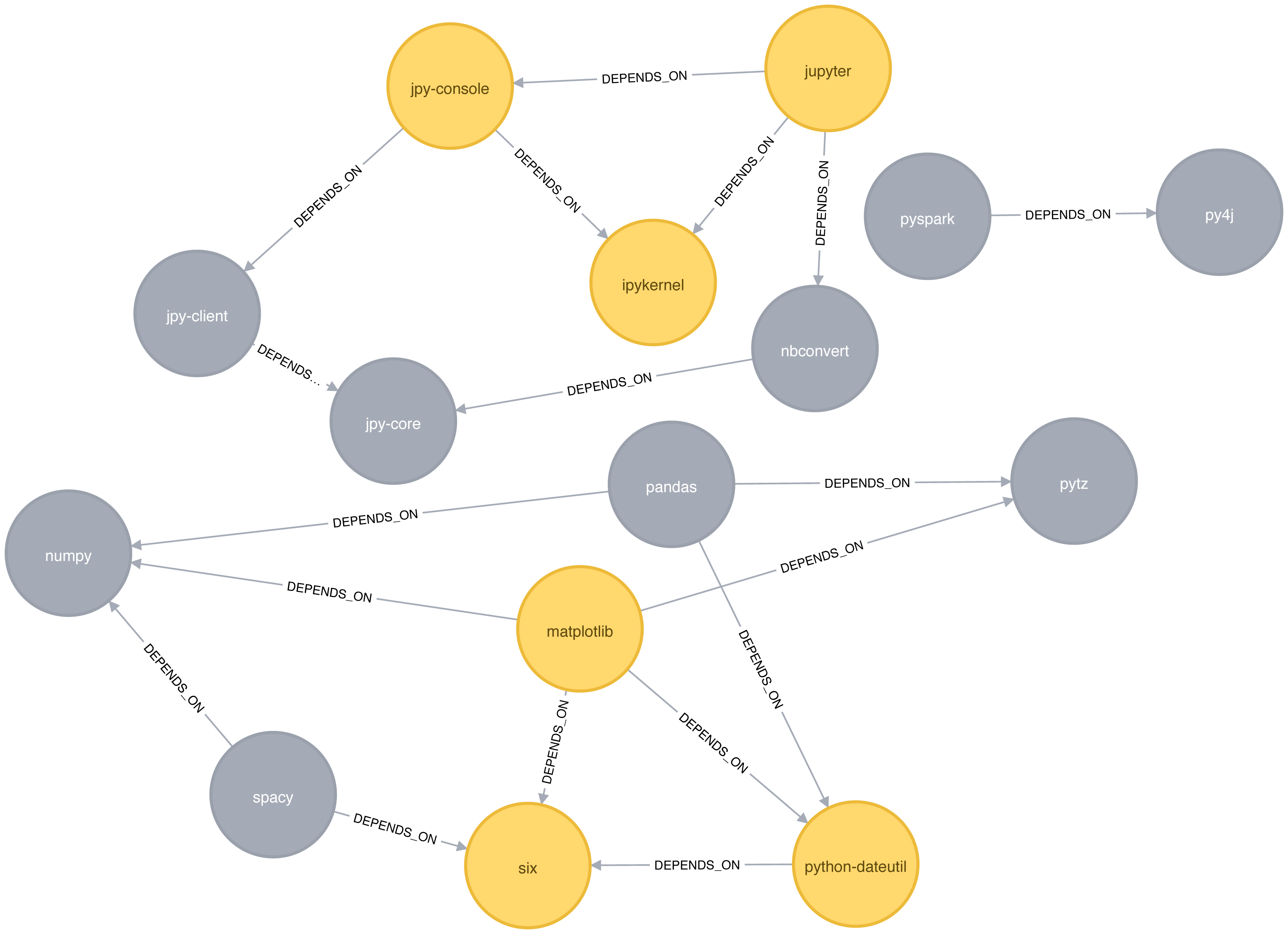
Figure 6-4. Triangles in the Software Dependency Graph
Local Clustering coefficient with Neo4j
We can also work out the local clustering coefficient. The following query will calculate this for each node:
CALL algo.triangleCount.stream('Library','DEPENDS_ON')YIELD nodeId, triangles, coefficientWHEREcoefficient > 0RETURNalgo.getNodeById(nodeId).idASlibrary, coefficientORDER BYcoefficientDESC
Running this procedure gives the following result:
| library | coefficient |
|---|---|
ipykernel |
1.0 |
jupyter |
0.3333333333333333 |
jpy-console |
0.3333333333333333 |
six |
0.3333333333333333 |
python-dateutil |
0.3333333333333333 |
matplotlib |
0.16666666666666666 |
ipykernel has a score of 1, which means that all ipykernel’s neighbors are neighbors of each other. We can clearly see that in Figure 6-4. This tells us that the community directly around ipykernel is very cohesive.
We’ve filtered out nodes with a coefficient score of 0 in this code sample, but nodes with low coefficients may also be interesting. A low score can be an indicator that a node is a structural hole. 7 A structural hole is a node that is well connected to nodes in different communities that aren’t otherwise connected to each other. This is another method for finding potential bridges, that we discussed last chapter.
Strongly Connected Components
The Strongly Connected Components (SCC) algorithm is one of the earliest graph algorithms. SCC finds sets of connected nodes in a directed graph where each node is reachable in both directions from any other node in the same set. It’s run-time operations scale well, proportional to the number of nodes. In Figure 6-5 you can see that the nodes in an SCC group don’t need to be immediate neighbors, but there must be directional paths between all nodes in the set.

Figure 6-5. Strongly Connected Components
Note
Decomposing a directed graph into its strongly connected components is a classic application of the Depth First Search algorithm. Neo4j uses DFS under the hood as part of its implementation of the SCC algorithm.
When Should I Use Strongly Connected Components?
Use Strongly Connected Components as an early step in graph analysis to see how our graph is structured or to identify tight clusters that may warrant independent investigation. A component that is strongly connected can be used to profile similar behavior or inclinations in a group for applications such as recommendation engines.
Many community detection algorithms like SCC are used to find and collapse clusters into single nodes for further inter-cluster analysis. You can also use SCC to visualize cycles for analysis like finding processes that might deadlock because each sub-process is waiting for another member to take action.
Example use cases include:
-
Finding the set of firms in which every member directly owns and/or indirectly owns shares in every other member, in the analysis of powerful transnational corporations 8.
-
Computing the connectivity of different network configurations when measuring routing performance in multihop wireless networks. Read more in Routing performance in the presence of unidirectional links in multihop wireless networks 9.
-
Acting as the first step in many graph algorithms that work only on strongly connected graphs. In social networks we find many strongly connected groups. In these sets, people often have similar preferences and the SCC algorithm is used to find such groups and suggest liked pages or purchased products to the people in the group who have not yet liked those pages or purchased those products.
Tip
Some algorithms have strategies for escaping infinite loops but if we’re writing our own algorithms or finding non-terminating processes, we canuse SCC to check for cycles.
Strongly Connected Components with Apache Spark
Starting with Apache Spark, we’ll first import the packages we need from Spark and the GraphFrames package.
fromgraphframesimport*frompyspark.sqlimportfunctionsasF
Now we’re ready to execute the Strongly Connected Components algorithm. We’ll use it to work out whether there are any circular dependencies in our graph.
Note
Two nodes can only be in the same strongly connected component if there are paths between them in both directions.
We write the following code to do this:
result=g.stronglyConnectedComponents(maxIter=10)result.sort("component")\.groupby("component")\.agg(F.collect_list("id").alias("libraries"))\.show(truncate=False)
If we run that code in pyspark we’ll see this output:
| component | libraries |
|---|---|
180388626432 |
[jpy-core] |
223338299392 |
[spacy] |
498216206336 |
[numpy] |
523986010112 |
[six] |
549755813888 |
[pandas] |
558345748480 |
[nbconvert] |
661424963584 |
[ipykernel] |
721554505728 |
[jupyter] |
764504178688 |
[jpy-client] |
833223655424 |
[pytz] |
910533066752 |
[python-dateutil] |
936302870528 |
[pyspark] |
944892805120 |
[matplotlib] |
1099511627776 |
[jpy-console] |
1279900254208 |
[py4j] |
You might notice that every library node is assigned to a unique component. This is the partition or subgroup it belongs to and as we (hopefully!) expected, every node is in its own partition. This means our software project has no circular dependencies amongst these libraries.
Strongly Connected Components with Neo4j
Let’s run the same algorithm using Neo4j. Execute the following query to run the algorithm:
CALL algo.scc.stream("Library","DEPENDS_ON")YIELD nodeId, partitionRETURNpartition,collect(algo.getNodeById(nodeId))ASlibrariesORDER BYsize(libraries)DESC
The parameters passed to this algorithm are:
-
Library- the node label to load from the graph -
DEPENDS_ON- the relationship type to load from the graph
This is the output we’ll see when we run the query:
| partition | libraries |
|---|---|
8 |
[ipykernel] |
11 |
[six] |
2 |
[matplotlib] |
5 |
[jupyter] |
14 |
[python-dateutil] |
13 |
[numpy] |
4 |
[py4j] |
7 |
[nbconvert] |
1 |
[pyspark] |
10 |
[jpy-core] |
9 |
[jpy-client] |
3 |
[spacy] |
12 |
[pandas] |
6 |
[jpy-console] |
0 |
[pytz] |
As with the Apache Spark example, every node is in it’s own partition.
So far the algorithm has only revealed that our Python libraries are very well behaved, but let’s create a circular dependency in the graph to make things more interesting. This should mean that we’ll end up with some nodes in the same partition.
The following query adds an extra library that creates a circular dependency between py4j and pyspark:
MATCH(py4j:Library {id:"py4j"})MATCH(pyspark:Library {id:"pyspark"})MERGE (extra:Library {id:"extra"})MERGE (py4j)-[:DEPENDS_ON]->(extra)MERGE (extra)-[:DEPENDS_ON]->(pyspark)
We can clearly see the circular dependency that got created in Figure 6-6
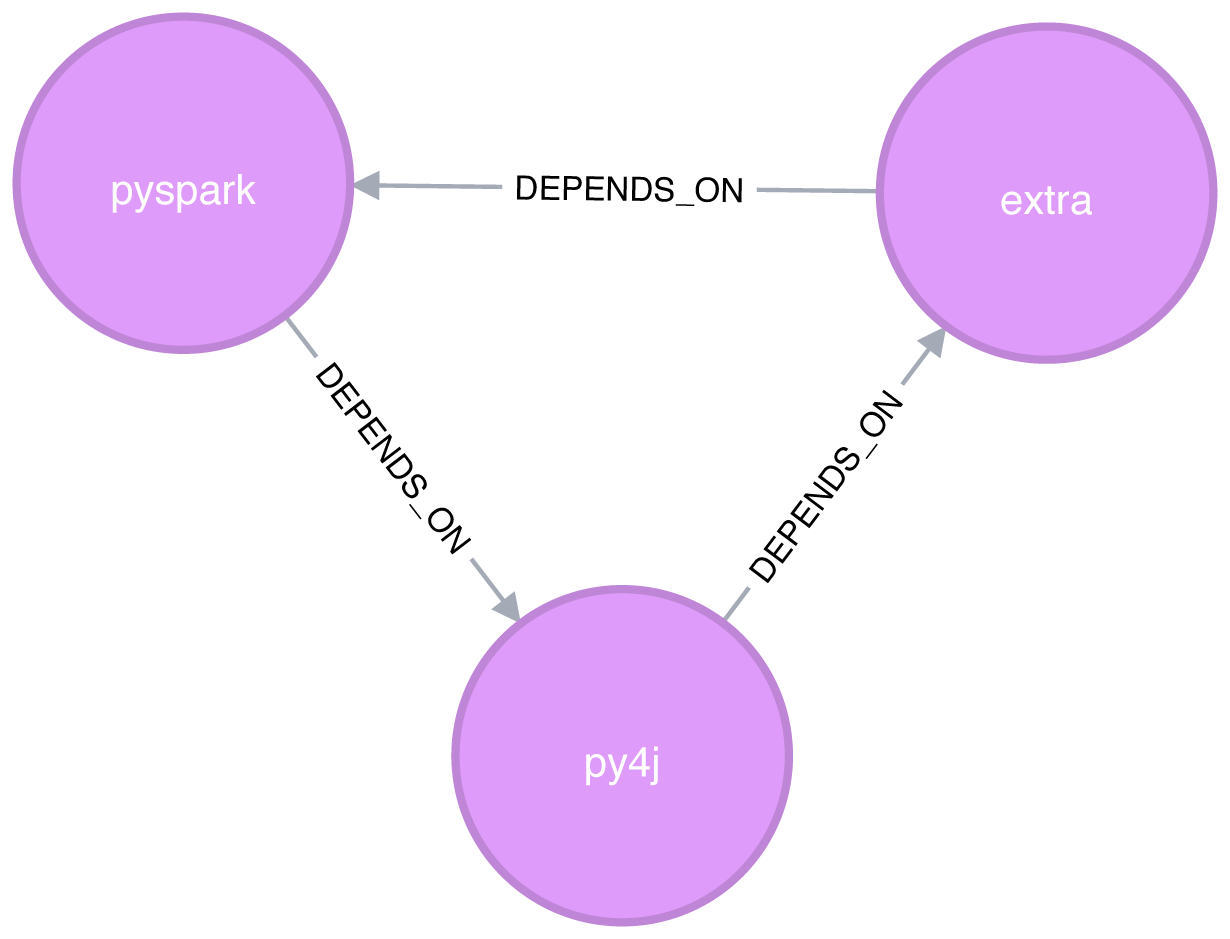
Figure 6-6. Circular dependency between pyspark, py4j, and extra
Now if we run the Strongly Connected Components algorithm again we’ll see a slightly different result:
| partition | libraries |
|---|---|
1 |
[pyspark, py4j, extra] |
8 |
[ipykernel] |
11 |
[six] |
2 |
[matplotlib] |
5 |
[jupyter] |
14 |
[numpy] |
13 |
[pandas] |
7 |
[nbconvert] |
10 |
[jpy-core] |
9 |
[jpy-client] |
3 |
[spacy] |
15 |
[python-dateutil] |
6 |
[jpy-console] |
0 |
[pytz] |
pyspark, py4j, and extra are all part of the same partition, and Strongly Connected Components has helped find the circular dependency!
Before we move onto the next algorithm we’ll delete the extra library and its relationships from the graph:
MATCH(extra:Library {id:"extra"})DETACHDELETEextra
Connected Components
The Connected Components algorithm finds sets of connected nodes in an undirected graph where each node is reachable from any other node in the same set (sometimes called Union Find or Weakly Connected Components). It differs from the Strongly Connected Components algorithm (SCC) because it only needs a path to exist between pairs of nodes in one direction, whereas SCC needs a path to exist in both directions.
Bernard A. Galler and Michael J. Fischer first described this algorithm in their 1964 paper, An improved equivalence algorithm 10.
When should I use Connected Components?
As with SCC, Connected Components is often used early in an analysis to understand a graph’s structure. Because it scales efficiently, consider this algorithm for graphs requiring frequent updates. It can quickly show new nodes in common between groups which is useful for analysis such as fraud detection.
Make it a habit to run Connected Components to test whether a graph is connected as a preparatory step for all our graph algorithms. Performing this quick test can avoid accidentally running algorithms on only one disconnected component of a graph and getting incorrect results.
Example use cases include:
-
Keeping track of clusters of database records, as part of the de-duplication process. Deduplication is an important task in master data management applications, and the approach is described in more detail in An Efficient Domain-Independent Algorithm for Detecting Approximately Duplicate Database Records 11.
-
Analyzing citation networks. One study uses Connected Components to work out how well-connected the network is, and then to see whether the connectivity remains if “hub” or “authority” nodes are moved from the graph. This use case is explained further in Characterizing and Mining Citation Graph of Computer Science Literature 12.
Connected Components with Apache Spark
Starting with Apache Spark, we’ll first import the packages we need from Spark and the GraphFrames package.
frompyspark.sqlimportfunctionsasF
Now we’re ready to execute the Connected Components algorithm.
Note
Two nodes can be in the same connected component if there is a path between them in either direction.
We write the following code to do this:
result=g.connectedComponents()result.sort("component")\.groupby("component")\.agg(F.collect_list("id").alias("libraries"))\.show(truncate=False)
If we run that code in pyspark we’ll see this output:
| component | libraries |
|---|---|
180388626432 |
[jpy-core, nbconvert, ipykernel, jupyter, jpy-client, jpy-console] |
223338299392 |
[spacy, numpy, six, pandas, pytz, python-dateutil, matplotlib] |
936302870528 |
[pyspark, py4j] |
The results show three clusters of nodes, which can also be seen visually in Figure 6-7.
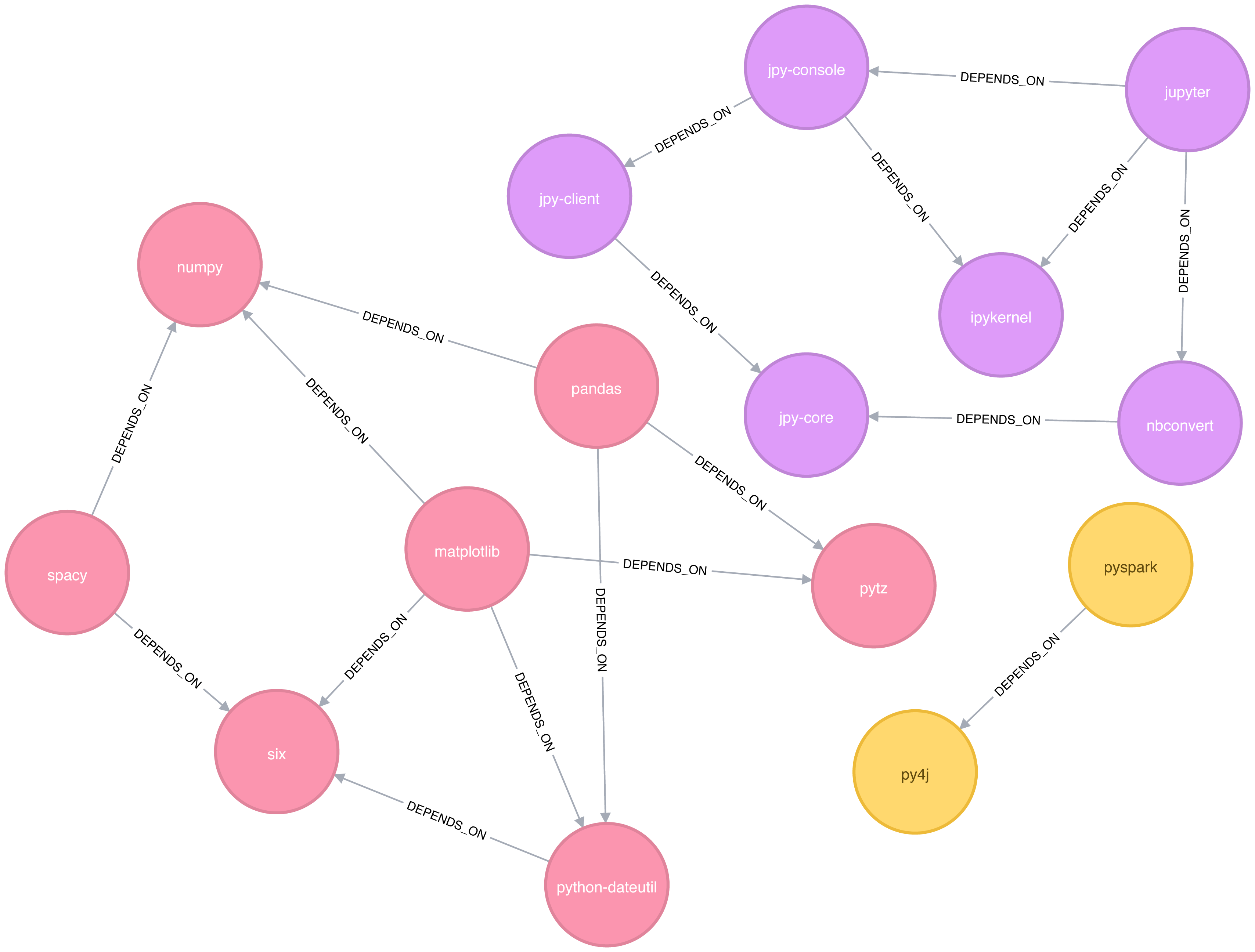
Figure 6-7. Clusters found by the Connected Components algorithm
In this example it’s very easy to see that there are 3 components just by visual inspection. This algorithm shows its value more on larger graphs where visual inspection isn’t possible or is very time consuming.
Connected Components with Neo4j
We can also execute this algorithm in Neo4j by running the following query:
CALL algo.unionFind.stream("Library","DEPENDS_ON")YIELD nodeId,setIdRETURNsetId,collect(algo.getNodeById(nodeId))ASlibrariesORDER BYsize(libraries)DESC
The parameters passed to this algorithm are:
-
Library- the node label to load from the graph -
DEPENDS_ON- the relationship type to load from the graph
This are the results:
| setId | libraries |
|---|---|
2 |
[pytz, matplotlib, spacy, six, pandas, numpy, python-dateutil] |
5 |
[jupyter, jpy-console, nbconvert, ipykernel, jpy-client, jpy-core] |
1 |
[pyspark, py4j] |
As expected, we get exactly the same results as we did with Apache Spark.
Both of the community detection algorithms that we’ve covered so far are deterministic: they return the same results each time we run them. Our next two algorithms are examples of non-deterministic algorithms, where we may see different results if we run them multiple times, even on the same data.
Label Propagation
The Label Propagation algorithm (LPA) is a fast algorithm for finding communities in a graph. In LPA, nodes select their group based on their direct neighbors. This process is well suited where groupings are less clear and weights can be used to help determine which community to place itself within. It also lends itself well to semi-supervised learning because you can seed the process with pre-assigned, indicative node labels.
The intuition behind this algorithm is that a single label can quickly become dominant in a densely connected group of nodes, but it will have trouble crossing a sparsely connected region. Labels get trapped inside a densely connected group of nodes, and nodes that end up with the same label when the algorithm finishes are considered part of the same community. The algorithm resolves overlaps, where nodes are potentially part of multiple clusters, by assigning membership to the label neighbourhood with the highest combined relationship and node weight.
LPA is a relatively new algorithm and was only proposed by Raghavan et al., in 2007, in a paper titled Near linear time algorithm to detect community structures in large-scale networks 13.
Figure 6-8 depicts 2 variations of Label Propagation, a simple push method and the more typical pull method that relies on relationship weights. The pull method lends itself well to parallelization.
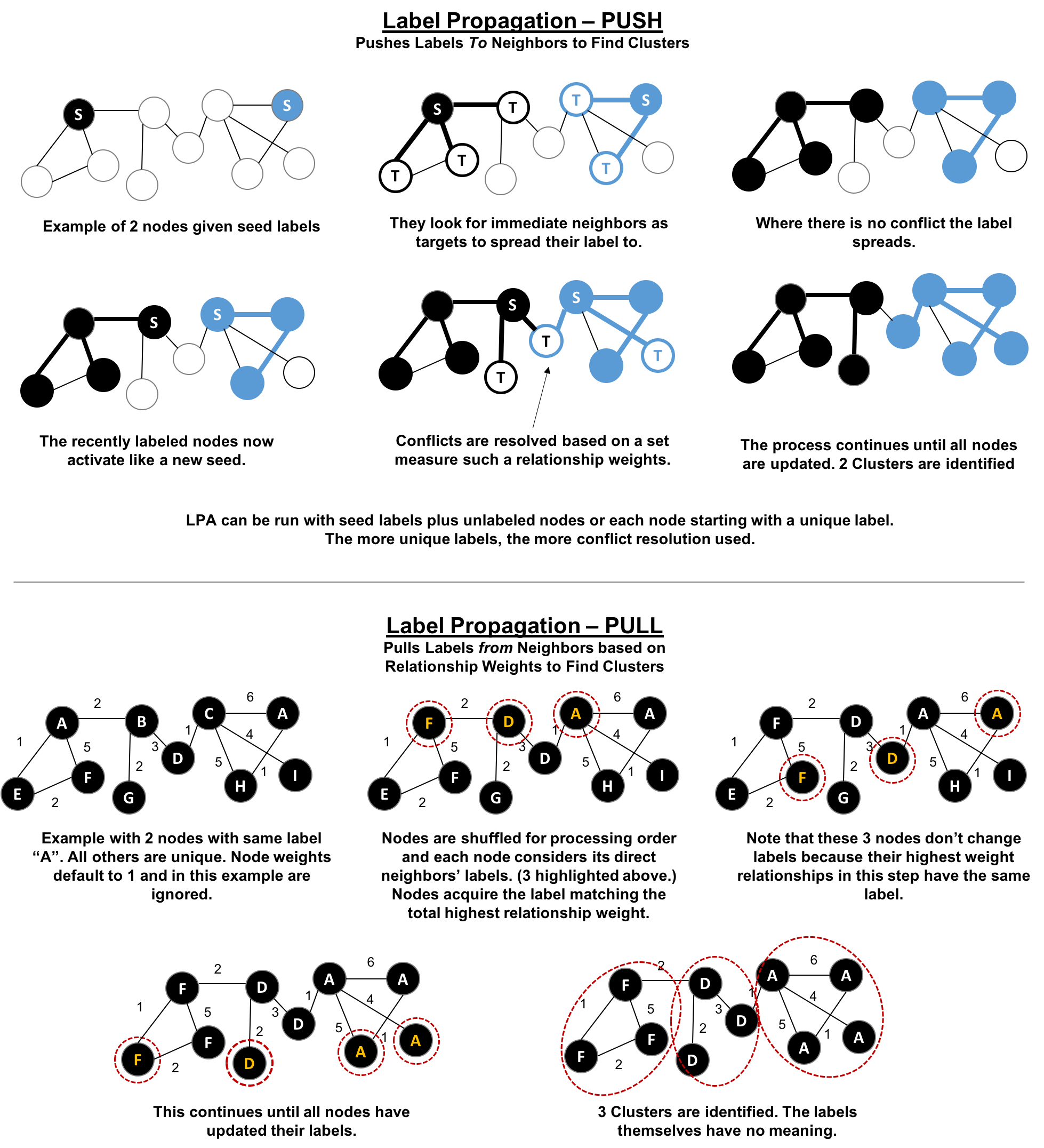
Figure 6-8. Two variations of Label Propation
The steps for the Label Propagation pull method often used are:
-
Every node is initialized with a unique label (an identifier).
-
These labels propagate through the network.
-
At every propagation iteration, each node updates its label to match the one with the maximum weight, which is calculated based on the weights of neighbor nodes and their relationships. Ties are broken uniformly and randomly.
-
LPA reaches convergence when each node has the majority label of its neighbors.
As labels propagate, densely connected groups of nodes quickly reach a consensus on a unique label. At the end of the propagation, only a few labels will remain, and nodes that have the same label belong to the same community.
Semi-Supervised Learning and Seed Labels
In contrast to other algorithms, Label Propagation can return different community structures when run multiple times on the same graph. The order in which LPA evaluates nodes can have an influence on the final communities it returns.
The range of solutions is narrowed when some nodes are given preliminary labels (i.e., seed labels), while others are unlabeled. Unlabeled nodes are more likely to adopt the preliminary labels.
This use of Label Propagation can be considered as a semi-supervised learning method to find communities. Semi-supervised learning is a class of machine learning tasks and techniques that operate on a small amount of labeled data, along with a larger amount of unlabeled data. We can also run the algorithm repeatedly on graphs as they evolve.
Finally, LPA sometimes doesn’t converge on a single solution. In this situation, our community results will continually flip between a few remarkably similar communities and would never complete. Seed labels help guide the algorithm towards a solution. Apache Spark and Neo4j set a maximum number of iterations to avoid never-ending execution. We should test the iteration setting for our data to balance accuracy and execution time.
When Should I Use Label Propagation?
Use Label Propagation in large-scale networks for initial community detection. This algorithm can be parallelised and is therefore extremely fast at graph partitioning.
Example use cases include:
-
Assigning polarity of tweets as a part of semantic analysis. In this scenario, positive and negative seed labels from a classifier are used in combination with the Twitter follower graph. For more information, see Twitter polarity classification with label propagation over lexical links and the follower graph 14.
-
Finding potentially dangerous combinations of possible co-prescribed drugs, based on the chemical similarity and side effect profiles. The study is found in Label Propagation Prediction of Drug-Drug Interactions Based on Clinical Side Effects 15.
-
Inferring dialogue features and user intention for a machine learning model. For more information, see Feature Inference Based on Label Propagation on Wikidata Graph for DST 16.
Label Propagation with Apache Spark
Starting with Apache Spark, we’ll first import the packages we need from Apache Spark and the GraphFrames package.
frompyspark.sqlimportfunctionsasF
Now we’re ready to execute the Label Propagation algorithm. We write the following code to do this:
result=g.labelPropagation(maxIter=10)result.sort("label").groupby("label").agg(F.collect_list("id")).show(truncate=False)
If we run that code in pyspark we’ll see this output:
| label | collect_list(id) |
|---|---|
180388626432 |
[jpy-core, jpy-console, jupyter] |
223338299392 |
[matplotlib, spacy] |
498216206336 |
[python-dateutil, numpy, six, pytz] |
549755813888 |
[pandas] |
558345748480 |
[nbconvert, ipykernel, jpy-client] |
936302870528 |
[pyspark] |
1279900254208 |
[py4j] |
Compared to Connected Components we have more clusters of libraries in this example. LPA is less strict than Connected Components with respect to how it determines clusters. Two neighbors (directly connected nodes) may be found to be in different clusters using Label Propagation. However, using Connected Components a node would always be in the same cluster as its neighbors because that algorithm bases grouping strictly on relationships.
In our example, the most obvious difference is that the Jupyter libraries have been split into two communities - one containing the core parts of the library and the other with the client facing tools.
Label Propagation with Neo4j
Now let’s try the same algorithm with Neo4j. We can execute LPA by running the following query:
CALL algo.labelPropagation.stream("Library","DEPENDS_ON",{ iterations: 10 })YIELD nodeId, labelRETURNlabel,collect(algo.getNodeById(nodeId).id)ASlibrariesORDER BYsize(libraries)DESC
The parameters passed to this algorithm are:
-
Library- the node label to load from the graph -
DEPENDS_ON- the relationship type to load from the graph -
iterations: 10- the maximum number of iterations to run
These are the results we’d see:
| label | libraries |
|---|---|
11 |
[matplotlib, spacy, six, pandas, python-dateutil] |
10 |
[jupyter, jpy-console, nbconvert, jpy-client, jpy-core] |
4 |
[pyspark, py4j] |
8 |
[ipykernel] |
13 |
[numpy] |
0 |
[pytz] |
The results, which can also be seen visually in Figure 6-9, are fairly similar to those we got with Apache Spark.
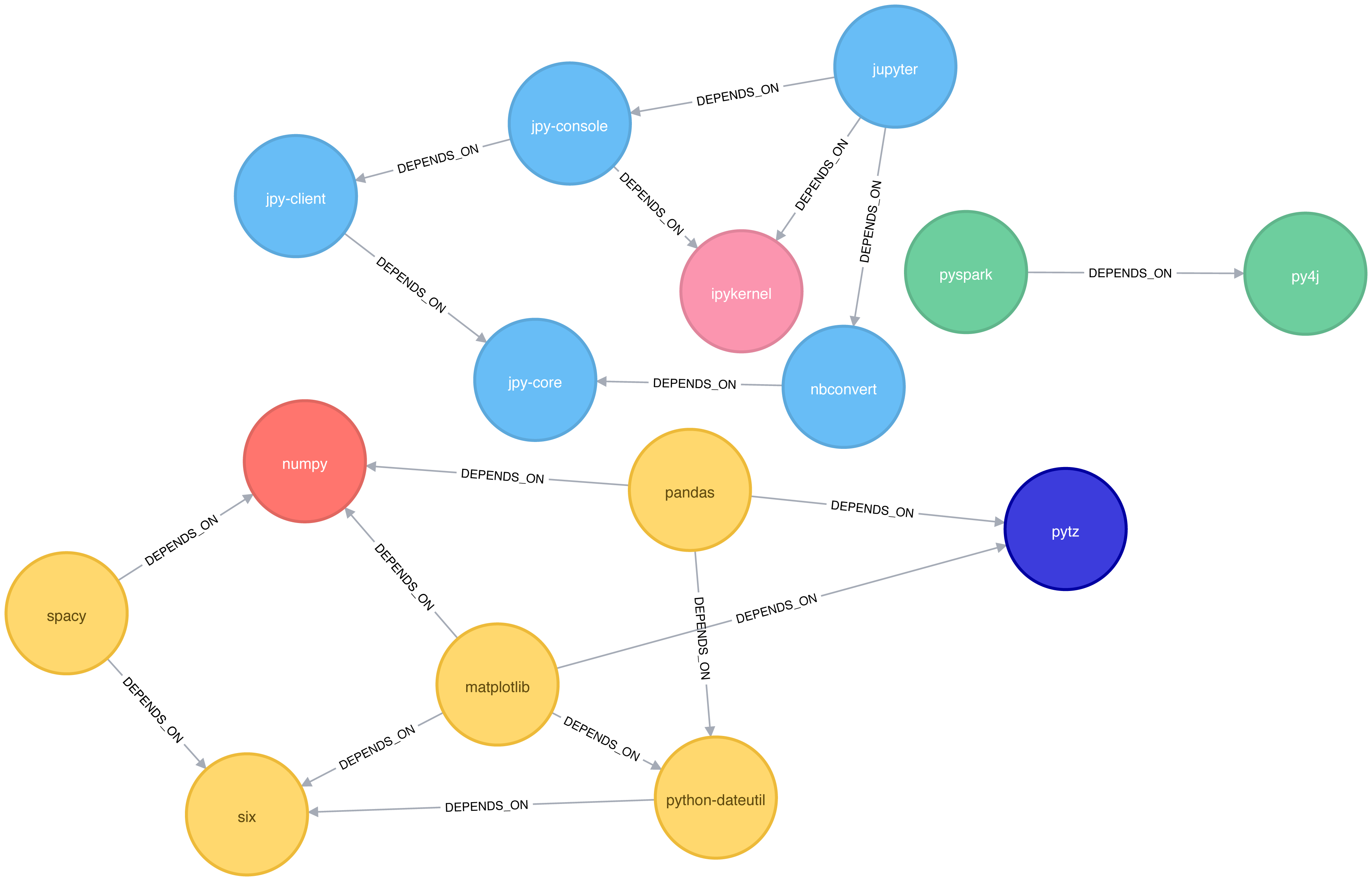
Figure 6-9. Clusters found by the Label Propagation algorithm
We can also run the algorithm assuming that the graph is undirected, which means that nodes will try and adopt the labels both of libraries they depend on as well as ones that depend on them.
To do this, we pass the DIRECTION:BOTH parameter to the algorithm:
CALL algo.labelPropagation.stream("Library","DEPENDS_ON",{ iterations: 10, direction:"BOTH"})YIELD nodeId, labelRETURNlabel,collect(algo.getNodeById(nodeId).id)ASlibrariesORDER BYsize(libraries)DESC
If we run that algorithm we’ll get the following output:
| label | libraries |
|---|---|
11 |
[pytz, matplotlib, spacy, six, pandas, numpy, python-dateutil] |
10 |
[nbconvert, jpy-client, jpy-core] |
6 |
[jupyter, jpy-console, ipykernel] |
4 |
[pyspark, py4j] |
The number of clusters has reduced from 6 to 4, and all the nodes in the matplotlib part of the graph are now grouped together. This can be seen more clearly in Figure 6-10.
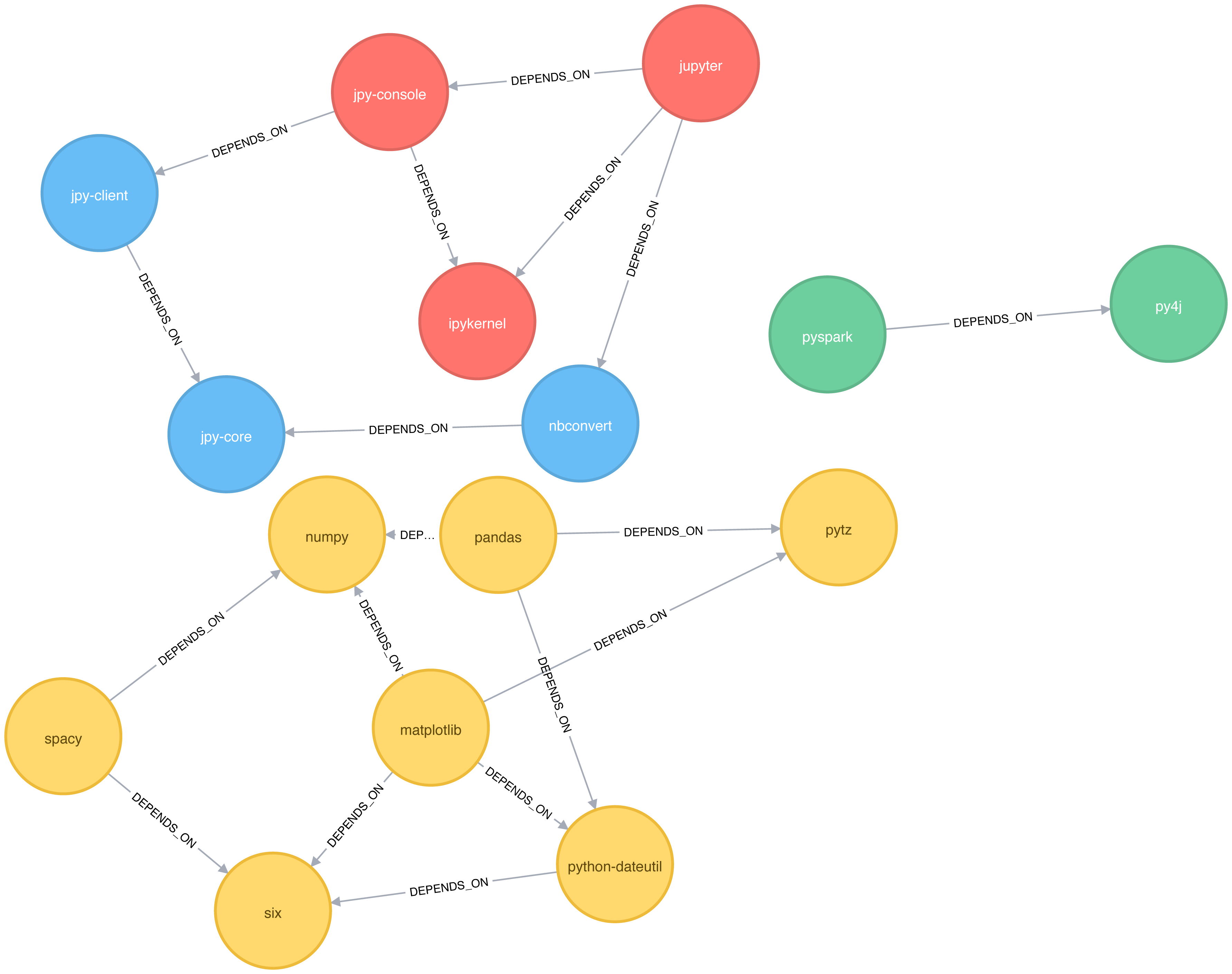
Figure 6-10. Clusters found by the Label Propagation algorithm, when ignoring relationship direction
Although the results of running Label Propagation on this data are similiar for undirected and directed calculation, on complicated graphs you will see more significant differences. This is because ignoring direction causes nodes to try and adopt the labels both of libraries they depend on as well as ones that depend on them.
Louvain Modularity
The Louvain Modularity algorithm finds clusters by comparing community density as it assigns nodes to different groups. You can think of this as a “what if” analysis to try out various grouping with the goal of eventually reaching a global optimum.
The Louvain algorithm 17 was proposed in 2008, and is one of the fastest modularity-based algorithms. As well as detecting communities, it also reveals a hierarchy of communities at different scales. This is useful for understanding the structure of a network at different levels of granularity.
Lovain quantifies how well a node is assigned to group by looking at the density of connections within a cluster in comparison to an average or random sample. This measure of community assignment is called modularity.
Quality based grouping via modularity
Modularity is a technique for uncovering communities by partitioning a graph into more coarse-grained modules (or clusters) and then measuring the strength of the groupings. As opposed to just looking at the concentration of connections within a cluster, this method compares relationship densities in given clusters to densities between clusters. The measure of the quality of those groupings is called modularity.
Modularity algorithms optimize communities locally and then globally, using multiple iterations to test different groupings and increasing coarseness. This strategy identifies community hierarchies and provides a broad understanding of the overall structure. However, all modularity algorithms suffer from two drawbacks:
1) they merge smaller communities into larger ones 2) a plateau where several partition options with similar modularity forming local maxima and preventing progress.
For more information, see “The performance of modularity maximization in practical contexts .”18 Remember that communities evolve and change over time so comparative analysis can help predict whether your groups are growing, merging, splitting or shrinking.
1 https://github.com/neo4j-graph-analytics/book/blob/master/data/sw-nodes.csv
2 https://github.com/neo4j-graph-analytics/book/blob/master/data/sw-relationships.csv
3 https://github.com/neo4j-graph-analytics/book
4 http://chato.cl/papers/becchetti_2007_approximate_count_triangles.pdf
5 https://arxiv.org/pdf/1111.4503.pdf
6 http://www.pnas.org/content/99/9/5825
7 http://theory.stanford.edu/~tim/s14/l/l1.pdf
8 http://journals.plos.org/plosone/article/file?id=10.1371/journal.pone.0025995&type=printable
9 https://dl.acm.org/citation.cfm?id=513803
10 https://dl.acm.org/citation.cfm?doid=364099.364331
11 http://citeseerx.ist.psu.edu/viewdoc/summary?doi=10.1.1.28.8405
12 https://pdfs.semanticscholar.org/a8e0/5f803312032569688005acadaa4d4abf0136.pdf
13 https://arxiv.org/pdf/0709.2938.pdf
14 https://dl.acm.org/citation.cfm?id=2140465
15 https://www.nature.com/articles/srep12339
16 https://www.uni-ulm.de/fileadmin/website_uni_ulm/iui.iwsds2017/papers/IWSDS2017_paper_12.pdf
17 https://arxiv.org/pdf/0803.0476.pdf
18 https://arxiv.org/abs/0910.0165
19 https://docs.lib.purdue.edu/cgi/viewcontent.cgi?article=1871&context=open_access_theses