Table of Contents for
Graph Algorithms
 Graph Algorithms
Published by
O'Reilly Media, Inc., 2019
Graph Algorithms
Published by
O'Reilly Media, Inc., 2019
- Cover
- nav
- Graph Algorithms
- Graph Algorithms
- Preface
- 1. Introduction
- 2. Graph Theory and Concepts
- 3. Graph Platforms and Processing
- 4. Pathfinding and Graph Search Algorithms
- 5. Centrality Algorithms
- 6. Community Detection Algorithms
- 7. Graph Algorithms in Practice
- 8. Using Graph Algorithms to Enhance Machine Learning
- About the Authors
Chapter 4. Pathfinding and Graph Search Algorithms
Pathfinding and Graph Search algorithms are used to identify optimal routes through a graph, and are often a required first step for many other types of analysis. In this chapter we’ll explain how these algorithms work and show examples in Spark and Neo4j. In cases where an algorithm is only available in one platform, we’ll provide just that one example or illustrate how you can customize your implementation.
Graph search algorithms explore a graph either for general discovery or explicit search. These algorithms carve paths through the graph, but there is no expectation that those paths are computationally optimal. In this chapter we will go into detail on the two types of of graph search algorithms, Breadth First Search and Depth First Search because they are so fundamental for traversing and searching a graph.
Pathfinding algorithms build on top of graph search algorithms and explore routes between nodes, starting at one node and traversing through relationships until the destination has been reached. These algorithms find the cheapest path in terms of the number of hops or weight. Weights can be anything measured, such as time, distance, capacity, or cost.
Specifically the algorithms we’ll cover are:
-
Shortest Path with 2 useful variations (A* and Yen’s) for finding the shortest path or paths between two chosen nodes
-
Single Source Shortest Path for finding the shortest path from a chosen node to all others
-
Minimum Spanning Tree for finding a connected tree structure with the smallest cost for visiting all nodes from a chosen node
-
Random Walk because it’s a useful pre-processing/sampling step for machine learning workflows and other graph algorithms
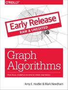
Figure 4-1 shows the key differences between these types of algorithms and Table 4-1 is a quick reference to what each algorithm computes with an example use.
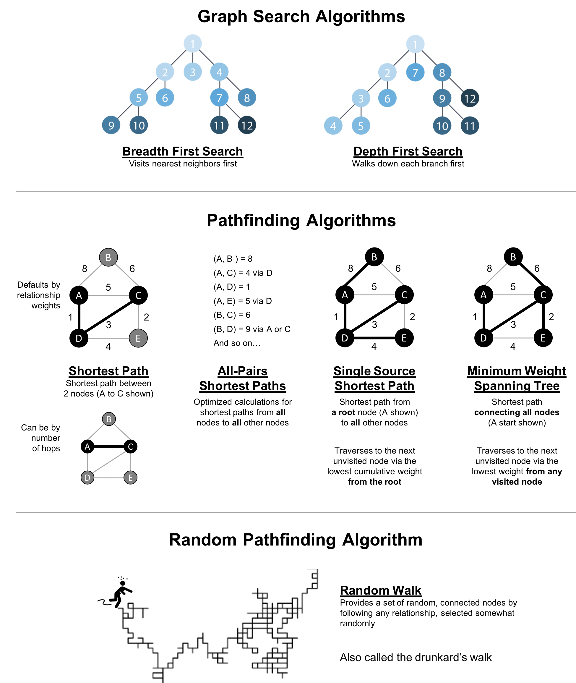
Figure 4-1. Pathfinding and Search Algorithms
| Algorithm Type | What It Does | Example Uses | Spark Example | Neo4j Example |
|---|---|---|---|---|
Traverses a tree structure by fanning out to explore the nearest neighbors and then their sub-level neighbors. |
Locate neighbor nodes in GPS systems to identify nearby places of interest. |
Yes |
No |
|
Traverses a tree structure by exploring as far as possible down each branch before backtracking. |
Discover an optimal solution path in gaming simulations with hierarchical choices. |
No |
No |
|
Calculates the shortest path between a pair of nodes. |
Find driving directions between two locations. |
Yes |
Yes |
|
Calculates the shortest path between all pairs of nodes in the graph. |
Evaluate alternate routes around a traffic jam. |
Yes |
Yes |
|
Calculates the shorest path between a single root node and all other nodes. |
Least cost routing of phone calls. |
Yes |
Yes |
|
Calculates the path in a connected tree structure with the smallest cost for visiting all nodes. |
Optimize connected routing such as laying cable or garbage collection. |
No |
Yes |
|
Returns a list of nodes along a path of specified size by randomly choosing relationships to traverse. |
Augment training for machine learning or data for graph algorithms. |
No |
Yes |
First we’ll take a look at the dataset for our examples and walk through how to import the data into Apache Spark and Neo4j. For each algorithm, we’ll start with a short description of the algorithm and any pertinent information on how it operates. Most sections also include guidance on when to use any related algorithms. Finally we provide working sample code using a sample dataset at the end of each section.
Let’s get started!
Example Data: The Transport Graph
All connected data contains paths between nodes and transportation datasets show this in an intuitive and accessible way. The examples in this chapter run against a graph containing a subset of the European road network 1. You can download the nodes 2 and relationships 3 files from the book’s GitHub repository 4.
transport-nodes.csv
| id | latitude | longitude | population |
|---|---|---|---|
Amsterdam |
52.379189 |
4.899431 |
821752 |
Utrecht |
52.092876 |
5.104480 |
334176 |
Den Haag |
52.078663 |
4.288788 |
514861 |
Immingham |
53.61239 |
-0.22219 |
9642 |
Doncaster |
53.52285 |
-1.13116 |
302400 |
Hoek van Holland |
51.9775 |
4.13333 |
9382 |
Felixstowe |
51.96375 |
1.3511 |
23689 |
Ipswich |
52.05917 |
1.15545 |
133384 |
Colchester |
51.88921 |
0.90421 |
104390 |
London |
51.509865 |
-0.118092 |
8787892 |
Rotterdam |
51.9225 |
4.47917 |
623652 |
Gouda |
52.01667 |
4.70833 |
70939 |
transport-relationships.csv
| src | dst | relationship | cost |
|---|---|---|---|
Amsterdam |
Utrecht |
EROAD |
46 |
Amsterdam |
Den Haag |
EROAD |
59 |
Den Haag |
Rotterdam |
EROAD |
26 |
Amsterdam |
Immingham |
EROAD |
369 |
Immingham |
Doncaster |
EROAD |
74 |
Doncaster |
London |
EROAD |
277 |
Hoek van Holland |
Den Haag |
EROAD |
27 |
Felixstowe |
Hoek van Holland |
EROAD |
207 |
Ipswich |
Felixstowe |
EROAD |
22 |
Colchester |
Ipswich |
EROAD |
32 |
London |
Colchester |
EROAD |
106 |
Gouda |
Rotterdam |
EROAD |
25 |
Gouda |
Utrecht |
EROAD |
35 |
Den Haag |
Gouda |
EROAD |
32 |
Hoek van Holland |
Rotterdam |
EROAD |
33 |
Figure 4-2 shows the target graph that we want to construct:
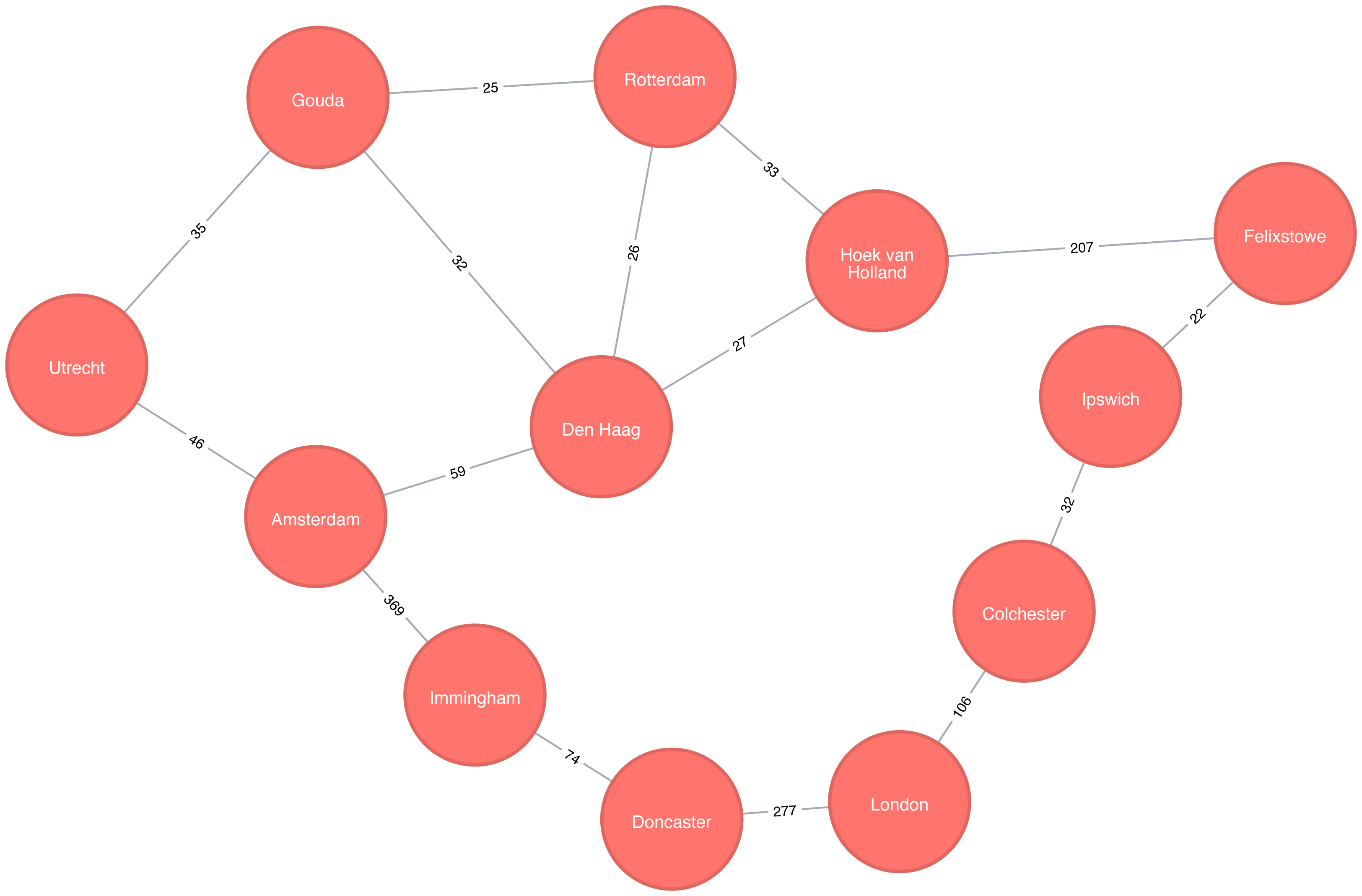
Figure 4-2. Transport Graph
For simplicity we consider the graph in Figure 4-2 to be undirected because most roads between cities are bidirectional. We’d get slightly different results if we evaluated the graph as directed because of the small number of one-way streets, but the overall approach remains similar. Conversely, both Apache Spark and Neo4j operate on directed graphs. In cases like this where we want to work with undirected graphs (bidirectional roads) there is an easy workaround:
-
For Apache Spark we’ll create two relationships for each row in
transport-relationships.csv- one going fromdsttosrcand one fromsrctodst. -
For Neo4j we’ll create a single relationship and then ignore the relationship direction when we run the algorithms.
Having understood those little modeling workarounds, we can now get on with loading graphs into Apache Spark and Neo4j from the example CSV files.
Importing the data into Apache Spark
Starting with Apache Spark, we’ll first import the packages we need from Spark and the GraphFrames package.
frompyspark.sql.typesimport*fromgraphframesimport*
The following function creates a GraphFrame from the example CSV files:
defcreate_transport_graph():node_fields=[StructField("id",StringType(),True),StructField("latitude",FloatType(),True),StructField("longitude",FloatType(),True),StructField("population",IntegerType(),True)]nodes=spark.read.csv("data/transport-nodes.csv",header=True,schema=StructType(node_fields))rels=spark.read.csv("data/transport-relationships.csv",header=True)reversed_rels=rels.withColumn("newSrc",rels.dst)\.withColumn("newDst",rels.src)\.drop("dst","src")\.withColumnRenamed("newSrc","src")\.withColumnRenamed("newDst","dst")\.select("src","dst","relationship","cost")relationships=rels.union(reversed_rels)returnGraphFrame(nodes,relationships)
Loading the nodes is easy, but for the relationships we need to do a little preprocessing so that we can create each relationship twice.
Now let’s call that function:
g=create_transport_graph()
Importing the data into Neo4j
Now for Neo4j. We’ll start by loading the nodes:
WITH"https://github.com/neo4j-graph-analytics/book/raw/master/data/transport-nodes.csv"ASuriLOAD CSVWITHHEADERS FROM uriASrowMERGE (place:Place {id:row.id})SETplace.latitude = toFloat(row.latitude),place.longitude = toFloat(row.latitude),place.population = toInteger(row.population)
And now the relationships:
WITH"https://github.com/neo4j-graph-analytics/book/raw/master/data/transport-relationships.csv"ASuriLOAD CSVWITHHEADERS FROM uriASrowMATCH(origin:Place {id: row.src})MATCH(destination:Place {id: row.dst})MERGE (origin)-[:EROAD {distance: toInteger(row.cost)}]->(destination)
Although we’re storing a directed relationship we’ll ignore the direction when we execute algorithms later in the chapter.
Breadth First Search
Breadth First Search (BFS) is one of the fundamental graph traversal algorithms. It starts from a chosen node and explores all of its neighbors at one hop away before visiting all neighbors at two hops away and so on.
The algorithm was first published in 1959 by Edward F. Moore who used it to find the shortest path out of a maze. It was later developed into a wire routing algorithm by C. Y. Lee in 1961 as described in “An Algorithm for Path Connections and Its Applications” 5
It is most commonly used as the basis for other more goal-oriented algorithms. For example Shortest Path, Connected Components, and Closeness Centrality all use the BFS algorithm. It can also be used to find the shortest path between nodes.
Figure 4-3 shows the order that we would visit the nodes of our transport graph if we were performing a breadth first search that started from Den Haag (in English, the Dutch city of The Hague). We first visit all of Den Haag’s direct neighbors, before visiting their neighbors, and their neighbors neighbors, until we’ve run out of relationships to traverse.
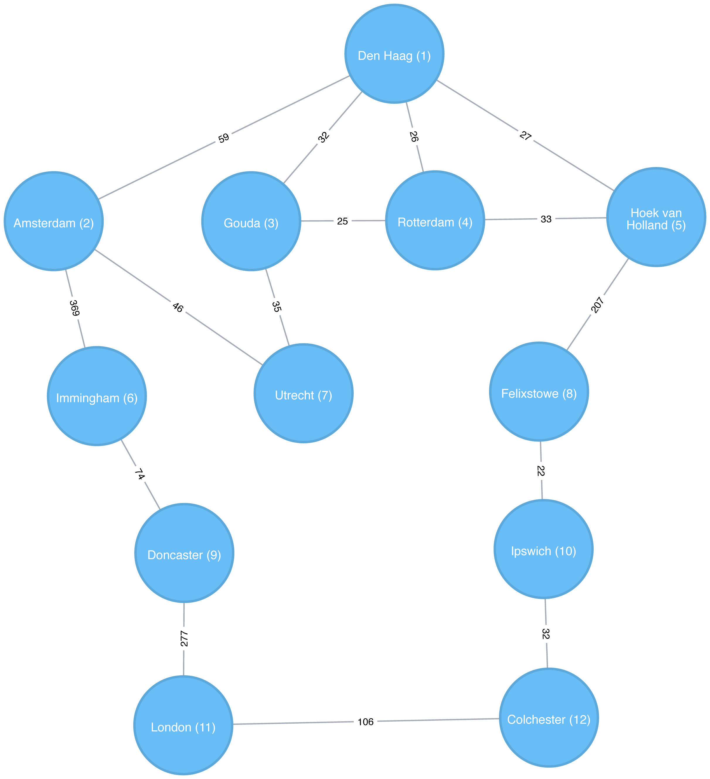
Figure 4-3. Breadth First Search starting from Den Haag, node numbers indicate the order traversed
Breadth First Search with Apache Spark
Apache Spark’s implementation of the Breadth First Search algorithm finds the shortest path between two nodes by the number of relationships (i.e. hops) between them. You can explicitly name your target node or add a criteria to be met.
For example, we can use the bfs function to find the first medium sized (by European standards) city that has a population of between 100,000 and 300,000 people.
Let’s first check which places have a population matching that criteria:
g.vertices\.filter("population > 100000 and population < 300000")\.sort("population")\.show()
This is the output we’ll see:
| id | latitude | longitude | population |
|---|---|---|---|
Colchester |
51.88921 |
0.90421 |
104390 |
Ipswich |
52.05917 |
1.15545 |
133384 |
There are only two places matching our criteria and we’d expect to reach Ipswich first based on a breadth first search.
The following code finds the shortest path from Den Haag to a medium-sized city:
from_expr="id='Den Haag'"to_expr="population > 100000 and population < 300000 and id <> 'Den Haag'"result=g.bfs(from_expr,to_expr)
result contains columns that describe the nodes and relationships between the two cities.
We can run the following code to see the list of columns returned:
(result.columns)
This is the output we’ll see:
['from', 'e0', 'v1', 'e1', 'v2', 'e2', 'to']
Columns beginning with e represent relationships (edges) and columns beginning with v represent nodes (vertices).
We’re only interested in the nodes so let’s filter out any columns that begin with e from the resulting DataFrame.
columns=[columnforcolumninresult.columnsifnotcolumn.startswith("e")]result.select(columns).show()
If we run the code in pyspark we’ll see this output:
| from | v1 | v2 | to |
|---|---|---|---|
[Den Haag, 52.078… |
[Hoek van Holland… |
[Felixstowe, 51.9… |
[Ipswich, 52.0591… |
As expected the bfs algorithm returns Ipswich!
Remember that this function is satisfied when it finds the first matching criteria and as you can see in Figure 4-3, Ipswich is evaluated before Colchester.
Depth First Search
Depth First Search (DFS) is the other fundamental graph traversal algorithm. It was originally invented by French mathematician Charles Pierre Trémaux as a strategy for solving mazes. It starts from a chosen node, picks one of its neighbors and then traverses as far as it can along that path before backtracking.
Figure 4-4 shows the order that we would visit the nodes of our transport graph if we were performing a DFS that started from Den Haag. We start by traversing from Den Haag to Amsterdam, and are then able to get to every other node in the graph without needing to backtrack at all!

Figure 4-4. Depth First Search starting from Den Haag, node numbers indicate the order traversed
Shortest Path
The Shortest Path algorithm calculates the shortest (weighted) path between a pair of nodes. It’s useful for user interactions and dynamic workflows because it works in real-time.
Pathfinding has a history dating back to the 19th century and is considered to be a classic graph problem. It gained prominence in the early 1950s in the context of alternate routing, that is, finding the second shortest route if the shortest route is blocked. In 1956, Edsger Dijkstra created the most well known of the shortest path algorithms.
Dijkstra’s Shortest Path operates by first finding the lowest weight relationship from the start node to directly connected nodes. It keeps track of those weights and moves to the “closest” node. It then performs the same calculation but now as a cumulative total from the start node. The algorithm continues to do this, evaluating a “wave” of cumulative weights and always choosing the lowest cumulative path to advance along. It reaches the destination node.
Note
You’ll notice in graph analytics the use of the terms weight, cost, distance, and hop when describing relationships and paths. “Weight” is the numeric value of a particular property of a relationship. “Cost” is similarly used but is more often when considering the total weight of a path.
“Distance” is often used within an algorithm as the name of the relationship property that indicates the cost of traversing between a pair of nodes. It’s not required that this be an actual physical measure of distance. “Hop” is commonly used to express the number of relationships between two nodes. You may see some of these terms combined such as, “it’s a 5-hop distance to London,” or, “that’s the lowest cost for the distance.”
When should I use Shortest Path?
Use Shortest Path to find optimal routes between a pair of nodes, based on either the number of hops or any weighted relationship value. For example, it can provide real-time answers about degrees of separation, the shortest distance between points, or the least expensive route. You can also use this algorithm to simply explore the connections between particular nodes.
Example use cases include:
-
Finding directions between locations: Web mapping tools such as Google Maps use the Shortest Path algorithm, or a close variant, to provide driving directions.
-
Social networks to find the degrees of separation between people. For example, when you view someone’s profile on LinkedIn, it will indicate how many people separate you in the graph, as well as listing your mutual connections.
-
The Bacon Number to find the number of degrees of separation between an actor and Kevin Bacon based on the movies they’ve appeared in. An example of this can be seen on the Oracle of Bacon 6 website. The Erdős Number Project 7 provides a similar graph analysis based on collaboration with Paul Erdős, one of the most prolific mathematicians of the 20th century.
Tip
Dijkstra does not support negative weights. The algorithm assumes that adding a relationship to a path can never make a path shorter—an invariant that would be violated with negative weights.
Shortest Path (weighted) with Apache Spark
In the Breadth First Search with Apache Spark section we learned how to find the shortest path between two nodes. That shortest path was based on hops and therefore isn’t the same as the shortest weighted path, which would tell us the shortest total distance between cities.
If we want to find the shortest weighted path (i.e. distance) we need to use the cost property, which is used for various types of weighting.
This option is not available out of the box with GraphFrames, so we need to write our own version of weighted shortest path using its aggregateMessages framework 8.
More information on aggregateMessages can be found in the Message passing via AggregateMessages 9 section of the GraphFrames user guide.
Tip
When available, we recommend you leverage pre-existing and tested libraries. Writing your own functions, especially for more complicated algorithms, require a deeper understanding of your data and calculations.
Before we create our function, we’ll import some libraries that we’ll use:
fromscripts.aggregate_messagesimportAggregateMessagesasAMfrompyspark.sqlimportfunctionsasF
The aggregate_messages module contains some useful helper functions.
It’s part of the GraphFrames library but isn’t available in a published artefact at the time of writing.
We’ve copied the module 10 into the book’s GitHub repository so that we can use it in our examples.
Now let’s write our function. We first create a User Defined Function that we’ll use to build the paths between our source and destination:
add_path_udf=F.udf(lambdapath,id:path+[id],ArrayType(StringType()))
And now for the main function which calculates the shortest path starting from an origin and returns as soon as the destination has been visited:
defshortest_path(g,origin,destination,column_name="cost"):ifg.vertices.filter(g.vertices.id==destination).count()==0:return(spark.createDataFrame(sc.emptyRDD(),g.vertices.schema).withColumn("path",F.array()))vertices=(g.vertices.withColumn("visited",F.lit(False)).withColumn("distance",F.when(g.vertices["id"]==origin,0).otherwise(float("inf"))).withColumn("path",F.array()))cached_vertices=AM.getCachedDataFrame(vertices)g2=GraphFrame(cached_vertices,g.edges)whileg2.vertices.filter('visited == False').first():current_node_id=g2.vertices.filter('visited == False').sort("distance").first().idmsg_distance=AM.edge[column_name]+AM.src['distance']msg_path=add_path_udf(AM.src["path"],AM.src["id"])msg_for_dst=F.when(AM.src['id']==current_node_id,F.struct(msg_distance,msg_path))new_distances=g2.aggregateMessages(F.min(AM.msg).alias("aggMess"),sendToDst=msg_for_dst)new_visited_col=F.when(g2.vertices.visited|(g2.vertices.id==current_node_id),True).otherwise(False)new_distance_col=F.when(new_distances["aggMess"].isNotNull()&(new_distances.aggMess["col1"]<g2.vertices.distance),new_distances.aggMess["col1"])\.otherwise(g2.vertices.distance)new_path_col=F.when(new_distances["aggMess"].isNotNull()&(new_distances.aggMess["col1"]<g2.vertices.distance),new_distances.aggMess["col2"].cast("array<string>"))\.otherwise(g2.vertices.path)new_vertices=(g2.vertices.join(new_distances,on="id",how="left_outer").drop(new_distances["id"]).withColumn("visited",new_visited_col).withColumn("newDistance",new_distance_col).withColumn("newPath",new_path_col).drop("aggMess","distance","path").withColumnRenamed('newDistance','distance').withColumnRenamed('newPath','path'))cached_new_vertices=AM.getCachedDataFrame(new_vertices)g2=GraphFrame(cached_new_vertices,g2.edges)ifg2.vertices.filter(g2.vertices.id==destination).first().visited:return(g2.vertices.filter(g2.vertices.id==destination).withColumn("newPath",add_path_udf("path","id")).drop("visited","path").withColumnRenamed("newPath","path"))return(spark.createDataFrame(sc.emptyRDD(),g.vertices.schema).withColumn("path",F.array()))
Tip
If we store references to any DataFrames in our functions we need to cache them using the AM.getCachedDataFrame function or we’ll encounter a memory leak when we execute the function.
In the shortest_path function we use this function to cache the vertices and new_vertices DataFrames.
If we want to find the shortest path between Amsterdam and Colchester we could call that function like so:
result=shortest_path(g,"Amsterdam","Colchester","cost")result.select("id","distance","path").show(truncate=False)
which would return the following results:
| id | distance | path |
|---|---|---|
Colchester |
347.0 |
[Amsterdam, Den Haag, Hoek van Holland, Felixstowe, Ipswich, Colchester] |
The total distance of the shortest path between Amsterdam and Colchester is 347 km and takes us via Den Haag, Hoek van Holland, Felixstowe, and Ipswich. By contrast the shortest path in terms of number of relationships between the locations, which we worked out with the Breadth First Search algorithm (refer back to Figure 4-4), would take us via Immingham, Doncaster, and London.
Shortest Path (weighted) with Neo4j
The Neo4j Graph Algorithms library also has a built-in shortest weighted path procedure that we can use.
Tip
All of Neo4j’s shortest path algorithms assume that the underlying graph is undirected.
You can override this by passing in the parameter direction: "OUTGOING" or direction: "INCOMING".
We can execute the weighted shortest path algorithm to find the shortest path between Amsterdam and London like this:
MATCH(source:Place {id:"Amsterdam"}),(destination:Place {id:"London"})CALL algo.shortestPath.stream(source, destination,"distance")YIELD nodeId, costRETURNalgo.getNodeById(nodeId).idASplace, cost
The parameters passed to this algorithm are:
-
source–the node where our shortest path search begins -
destination–the node where our shortest path ends -
distance–the name of the relationship property that indicates the cost of traversing between a pair of nodes.
The cost is the number of kilometers between two locations.
The query returns the following result:
| place | cost |
|---|---|
Amsterdam |
0.0 |
Den Haag |
59.0 |
Hoek van Holland |
86.0 |
Felixstowe |
293.0 |
Ipswich |
315.0 |
Colchester |
347.0 |
London |
453.0 |
The quickest route takes us via Den Haag, Hoek van Holland, Felixstowe, Ipswich, and Colchester! The cost shown is the cumulative total as we progress through cities. First, we go from Amsterdam to Den Haag, at a cost of 59. Then, we go from Den Haag to Hoek van Holland, at a cumulative cost of 86–and so on. Finally, we arrive from Colchester to London, for a total cost of 45 km.
We can also run an unweighted shortest path in Neo4j.
To have Neo4j’s shortest path algorithm do this we can pass null as the 3rd parameter to the procedure.
The algorithm will then assume a default weight of 1.0 for each relationship.
MATCH(source:Place {id:"Amsterdam"}),(destination:Place {id:"London"})CALL algo.shortestPath.stream(source, destination,null)YIELD nodeId, costRETURNalgo.getNodeById(nodeId).idASplace, cost
This query returns the following output:
| place | cost |
|---|---|
Amsterdam |
0.0 |
Immingham |
1.0 |
Doncaster |
2.0 |
London |
3.0 |
Here the cost is the cumulative total for relationships (or hops.) This is the same path as we would see using Breadth First Search in Spark.
We could even work out the total distance of following this path by writing a bit of post processing Cypher. The following procedure calculates the shortest unweighted path and then works out what the actual cost of that path would be:
MATCH(source:Place {id:"Amsterdam"}),(destination:Place {id:"London"})CALL algo.shortestPath.stream(source, destination,null)YIELD nodeId, costWITHcollect(algo.getNodeById(nodeId))ASpathUNWINDrange(0, size(path)-1)ASindexWITHpath[index]AScurrent, path[index+1]ASnextWITHcurrent, next, [(current)-[r:EROAD]-(next) | r.distance][0]ASdistanceWITHcollect({current: current, next:next, distance: distance})ASstopsUNWINDrange(0, size(stops)-1)ASindexWITHstops[index]ASlocation, stops, indexRETURNlocation.current.idASplace,reduce(acc=0.0,distancein[stopinstops[0..index] | stop.distance] |acc + distance)AScost
It’s a bit unwieldy-the tricky part is figuring out how to massage the data in such a way that we can see the cumulative cost over the whole journey. The query returns the following result:
| place | cost |
|---|---|
Amsterdam |
0.0 |
Immingham |
369.0 |
Doncaster |
443.0 |
London |
720.0 |
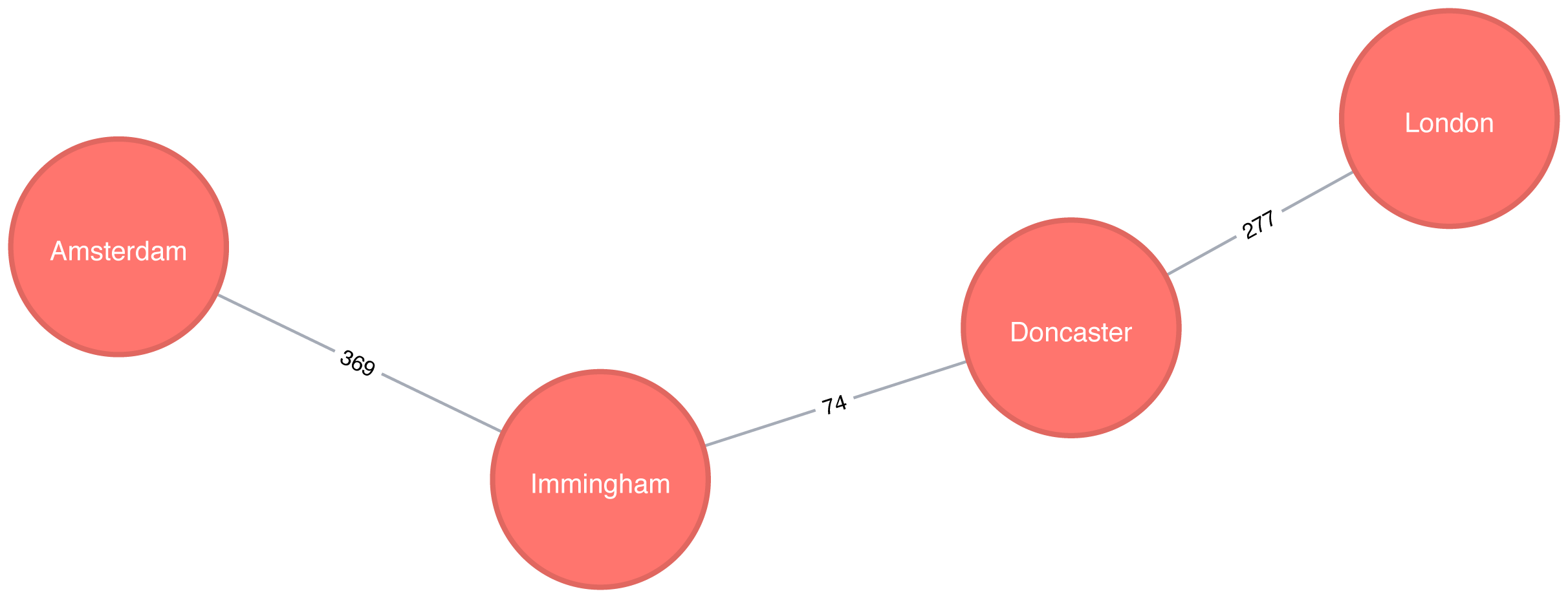
Figure 4-6. The unweighted shortest path between Amsterdam and London
Figure 4-6 shows the unweighted shortest path from Amsterdam to London. It has a total cost of 720 km, routing us through the fewest number of cities. The weighted shortest path, however, had a total cost of 453 km even though we visited more towns.
Shortest Path Variation: A*
The A* algorithm improves on Dijkstra’s algorithm, by finding shortest paths more quickly. It does this by allowing the inclusion of extra information that the algorithm can use, as part of a heuristic function, when determining which paths to explore next.
The algorithm was invented by Peter Hart, Nils Nilsson, and Bertram Raphael and described in their 1968 paper “A Formal Basis for the Heuristic Determination of Minimum Cost Paths” 11.
The A* algorithm operates by determining which of its partial paths to expand at each iteration of its main loop. It does so based on an estimate of the cost still to go to the goal node.
A* selects the path that minimizes the following function:
f(n) = g(n) + h(n)
where :
-
g(n)- the cost of the path from the starting point to noden. -
h(n)- the estimated cost of the path from nodento the destination node, as computed by a heuristic.
Note
In Neo4j’s implementation, geospatial distance is used as the heuristic. In our example transportation dataset we use the latitude and longitude of each location as part of the heuristic function.
A* with Neo4j
The following query executes the A* algorithm to find the shortest path between Den Haag and London:
MATCH(source:Place {id:"Den Haag"}),(destination:Place {id:"London"})CALL algo.shortestPath.astar.stream(source, destination,"distance","latitude","longitude")YIELD nodeId, costRETURNalgo.getNodeById(nodeId).idASplace, cost
The parameters passed to this algorithm are:
-
source-the node where our shortest path search begins -
destination-the node where our shortest path search ends -
distance-the name of the relationship property that indicates the cost of traversing between a pair of nodes. The cost is the number of kilometers between two locations. -
latitude-the name of the node property used to represent the latitude of each node as part of the geospatial heuristic calculation -
longitude-the name of the node property used to represent the longitude of each node as part of the geospatial heuristic calculation
Running this procedure gives the following result:
| place | cost |
|---|---|
Den Haag |
0.0 |
Hoek van Holland |
27.0 |
Felixstowe |
234.0 |
Ipswich |
256.0 |
Colchester |
288.0 |
London |
394.0 |
We’d get the same result using the Shortest Path algorithm, but on more complex datasets the A* algorithm will be faster as it evaluates fewer paths.
Shortest Path Variation: Yen’s K-shortest paths
Yen’s algorithm is similar to the shortest path algorithm, but rather than finding just the shortest path between two pairs of nodes, it also calculates the 2nd shortest path, 3rd shortest path, up to k-1 deviations of shortest paths.
Jin Y. Yen invented the algorithm in 1971 and described it in “Finding the K Shortest Loopless Paths in a Network” 12. This algorithm is useful for getting alternative paths when finding the absolute shortest path isn’t our only goal.
Yen’s with Neo4j
The following query executes the Yen’s algorithm to find the shortest paths between Gouda and Felixstowe.
MATCH(start:Place {id:"Gouda"}),(end:Place {id:"Felixstowe"})CALL algo.kShortestPaths.stream(start, end, 5,'distance')YIELD index, nodeIds, path, costsRETURNindex,[node inalgo.getNodesById(nodeIds[1..-1]) |node.id]ASvia,reduce(acc=0.0, costincosts | acc + cost)AStotalCost
The parameters passed to this algorithm are:
-
start-the node where our shortest path search begins -
end-the node where our shortest path search ends -
5-the maximum number of shortest paths to find -
distance-the name of the relationship property that indicates the cost of traversing between a pair of nodes. The cost is the number of kilometers between two locations.
After we get back the shortest paths we look up the associated node for each node id and then we filter out the start and end nodes from the collection.
Running this procedure gives the following result:
| index | via | totalCost |
|---|---|---|
0 |
[Rotterdam, Hoek van Holland] |
265.0 |
1 |
[Den Haag, Hoek van Holland] |
266.0 |
2 |
[Rotterdam, Den Haag, Hoek van Holland] |
285.0 |
3 |
[Den Haag, Rotterdam, Hoek van Holland] |
298.0 |
4 |
[Utrecht, Amsterdam, Den Haag, Hoek van Holland] |
374.0 |
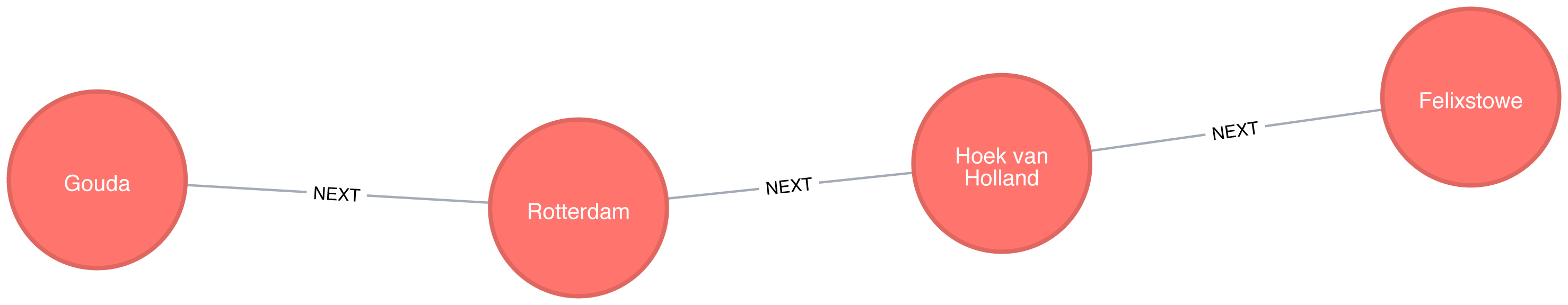
Figure 4-7. Shortest path between Gouda and Felixstowe
The shortest path between Gouda and Felixstowe in Figure 4-7 is interesting in comparison to the results ordered by total cost. It illustrates that sometimes you may want to consider several shortest paths or other parameters. In this example, the second shortest route is only 1 km longer than the shortest one. If we prefer the scenery, we might choose the slightly longer route.
All Pairs Shortest Paths
The All Pairs Shortest Path (APSP) calculates the shortest (weighted) path between all pairs of nodes. The algorithm can do this more quickly than calling the Single Source Shortest Path algorithm for every pair of nodes in the graph.
It optimizes operations by keeping track of the distances calculated so far and running on nodes in parallel. Those known distances can then be reused when calculating the shortest path to an unseen node. You can follow the example in the next section to get a better understanding of how the algorithm works.
Note
Some pairs of nodes might not be reachable from each other, which means that there is no shortest path between these nodes. The algorithm doesn’t return distances for these pairs of nodes.
A Closer Look at All Pairs Shortest Paths
The calculations for All Pairs Shortest Paths is easiest to understand when you follow a sequence of operations. The diagram in Figure 4-8 walks through the steps for A node calculations.
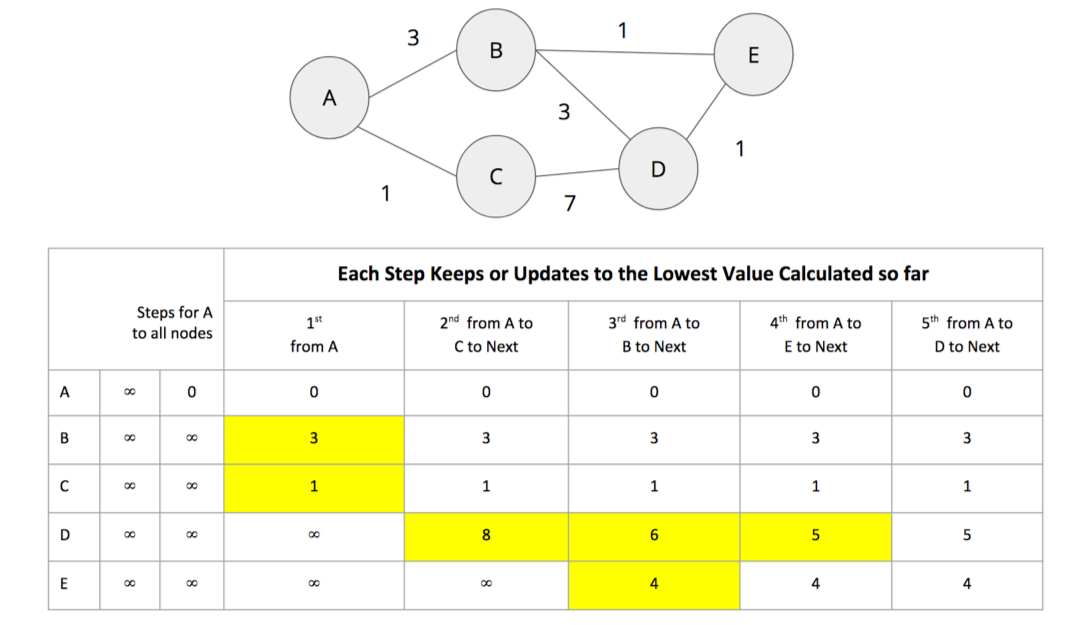
Figure 4-8. Calculating the shortest path from node A to everybody else
Initially the algorithm assumes an infinite distance to all nodes. When a start node is selected, then the distance to that node is set to 0.
From start node A we evaluate the cost of moving to the nodes we can reach and update those values. Looking for the smallest value, we have a choice of B (cost of 3) or C (cost of 1). C is selected for the next phase of traversal.
Now from node C, the algorithm updates the cumulative distances from A to nodes that can be reached directly from C. Values are only updated when a lower cost has been found:
A=0, B=3, C=1, D=8, E=∞
B is selected as the next closest node that hasn’t already been visited. B has relationships to nodes A, D, and E. The algorithm works out the distance to A, D, and E by summing the distance from A to B with the distance from B to those nodes. Note that the lowest cost from the start node (A) to the current node is always preserved as a sunk cost. The distance calculation results:
d(A,A) = d(A,B) + d(B,A) = 3 + 3 = 6
d(A,D) = d(A,B) + d(B,D) = 3 + 3 = 6
d(A,E) = d(A,B) + d(B,E) = 3 + 1 = 4
The distance for node A (6) – from node A to B and back – in this step is greater than the shortest distance already computed (0), so its value is not updated.
The distances for nodes D (6) and E (4) are less then the previously calculated distances, so their values are updated.
E is selected next and only the cumulative total for reaching D (5) is now lower and therefore is the only one updated. When D is finally evaluated, there are no new minimum path weights, nothign is updated, and the algorithm terminates.
Tip
Even though the All Pairs Shortest Paths algorithm is optimized to run calculations in parallel for each node, this can still add up for a very large graph. Consider using a subgraph if you only need to evaluate paths between a sub-category of nodes.
When should I use All Pairs Shortest Path?
All Pairs Shortest Path is commonly used for understanding alternate routing when the shortest route is blocked or becomes suboptimal. For example, this algorithm is used in logical route planning to ensure the best multiple paths for diversity routing. Use All Pairs Shortest Path when you need to consider all possible routes between all or most of your nodes.
Example use cases include:
-
Urban service problems, such as the location of urban facilities and the distribution of goods. One example of this is determining the traffic load expected on different segments of a transportation grid. For more information, see Urban Operations Research 13.
-
Finding a network with maximum bandwidth and minimal latency as part of a data center design algorithm. There are more details about this approach in the following academic paper: REWIRE: An Optimization-based Framework for Data Center Network Design 14.
All Pairs Shortest Paths with Apache Spark
Apache Spark’s shortestPaths function is designed for finding the path from all nodes to a set of nodes they call landmarks.
If we want to find the shortest path from every location to Colchester, Berlin, and Hoek van Holland, we write the following query:
result=g.shortestPaths(["Colchester","Immingham","Hoek van Holland"])result.sort(["id"]).select("id","distances").show(truncate=False)
If we run that code in pyspark we’ll see this output:
| id | distances |
|---|---|
Amsterdam |
[Immingham → 1, Hoek van Holland → 2, Colchester → 4] |
Colchester |
[Colchester → 0, Hoek van Holland → 3, Immingham → 3] |
Den Haag |
[Hoek van Holland → 1, Immingham → 2, Colchester → 4] |
Doncaster |
[Immingham → 1, Colchester → 2, Hoek van Holland → 4] |
Felixstowe |
[Hoek van Holland → 1, Colchester → 2, Immingham → 4] |
Gouda |
[Hoek van Holland → 2, Immingham → 3, Colchester → 5] |
Hoek van Holland |
[Hoek van Holland → 0, Immingham → 3, Colchester → 3] |
Immingham |
[Immingham → 0, Colchester → 3, Hoek van Holland → 3] |
Ipswich |
[Colchester → 1, Hoek van Holland → 2, Immingham → 4] |
London |
[Colchester → 1, Immingham → 2, Hoek van Holland → 4] |
Rotterdam |
[Hoek van Holland → 1, Immingham → 3, Colchester → 4] |
Utrecht |
[Immingham → 2, Hoek van Holland → 3, Colchester → 5] |
The number next to each location in the distances column is the number of relationships (roads) between cities we need to traverse to get there from the source node. In our example, Colchester is one of our destination cities and you can see it has 0 roads to traverse to get to itself but 3 hops to make from Immigham and Hoek van Holland.
All Pairs Shortest Paths with Neo4j
Neo4j has an implementation of All Pairs Shortest path which returns the distance between every pairs of nodes.
The first parameter to this procedure is the property to use to work out the shortest weighted path.
If we set this to null then the algorithm will calculate the non-weighted shortest path between all pairs of nodes.
The following query does this:
CALL algo.allShortestPaths.stream(null)YIELD sourceNodeId, targetNodeId, distanceWHEREsourceNodeId < targetNodeIdRETURNalgo.getNodeById(sourceNodeId).idASsource,algo.getNodeById(targetNodeId).idAStarget,distanceORDER BYdistanceDESCLIMIT10
This algorithm returns the shortest path between every pair of nodes twice - once with each of the nodes as the source node. This would be helpful if you were evaluting a directed graph of one way streets.
However, we don’t need to see each path twice so we filter the results to only keep one of them by using the sourceNodeId < targetNodeId predicate.
The query returns the following result:
| source | target | distance |
|---|---|---|
Colchester |
Utrecht |
5.0 |
London |
Rotterdam |
5.0 |
London |
Gouda |
5.0 |
Ipswich |
Utrecht |
5.0 |
Colchester |
Gouda |
5.0 |
Colchester |
Den Haag |
4.0 |
London |
Utrecht |
4.0 |
London |
Den Haag |
4.0 |
Colchester |
Amsterdam |
4.0 |
Ipswich |
Gouda |
4.0 |
This output shows the 10 pairs of locations that have the most relationships between them because we asked for results in descending order.
If we want to calculate the shortest weighted path, rather than passing in null as the first parameter, we can pass in the property name that contains the cost to be used in the shortest path calculation.
This property will then be evaluated to work out the shortest weighted path.
The following query does this:
CALL algo.allShortestPaths.stream("distance")YIELD sourceNodeId, targetNodeId, distanceWHEREsourceNodeId < targetNodeIdRETURNalgo.getNodeById(sourceNodeId).idASsource,algo.getNodeById(targetNodeId).idAStarget,distanceORDER BYdistanceDESCLIMIT10
The query returns the following result:
| source | target | distance |
|---|---|---|
Doncaster |
Hoek van Holland |
529.0 |
Rotterdam |
Doncaster |
528.0 |
Gouda |
Doncaster |
524.0 |
Felixstowe |
Immingham |
511.0 |
Den Haag |
Doncaster |
502.0 |
Ipswich |
Immingham |
489.0 |
Utrecht |
Doncaster |
489.0 |
London |
Utrecht |
460.0 |
Colchester |
Immingham |
457.0 |
Immingham |
Hoek van Holland |
455.0 |
Now we’re seeing the 10 pairs of locations furthest from each other in terms of the total distance between them.
Single Source Shortest Path
Single Source Shortest Path (SSSP), which came into prominence at the same time as the Shortest Path algorithm and Dijkstra’s algorithm, acts as an implementation for both problems.
The SSSP algorithm calculates the shortest (weighted) path from a root node to all other nodes in the graph, by executing the following steps:
-
It begins with a root node from which all paths will be measured.
-
Then the relationship with smallest weight coming from that root node is selected and added to the tree (along with its connected node).
-
Then the next relationship with smallest cumulative weight from your root node to any unvisited node is selected and added to the tree in the same way.
-
When there are no more nodes to add, you have your single source shortest path.
Figure 4-9 provides an example sequence.
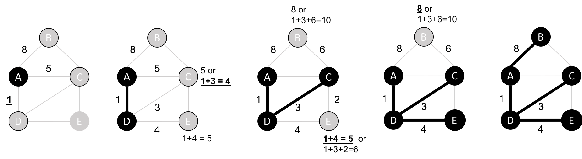
Figure 4-9. Single Source Shortest Path algorithm steps
When should I use Single Source Shortest Path?
Use Single Source Shortest Path when you need to evaluate the optimal route from a fixed start point to all other individual nodes. Because the route is chosen based on the total path weight from the root, it’s useful for finding the best path to each nodes but not necessarily when all nodes need to be visited in a single trip.
For example, identifying the main routes used for emergency services where you don’t visit every location on each incident versus a single route for garbage collection where you need to visit each house. (In the latter case, you’d use the Minimum Spanning Tree algorithm covered later.)
Example use case:
Single Source Shortest Path with Apache Spark
We can adapt the shortest path function that we wrote to calculate the shortest path between two locations to instead return us the shortest path from one location to all others.
We’ll first import the same libraries as before:
fromscripts.aggregate_messagesimportAggregateMessagesasAMfrompyspark.sqlimportfunctionsasF
And we’ll use the same User Defined function to construct paths:
add_path_udf=F.udf(lambdapath,id:path+[id],ArrayType(StringType()))
Now for the main function which calculates the shortest path starting from an origin:
defsssp(g,origin,column_name="cost"):vertices=g.vertices\.withColumn("visited",F.lit(False))\.withColumn("distance",F.when(g.vertices["id"]==origin,0).otherwise(float("inf")))\.withColumn("path",F.array())cached_vertices=AM.getCachedDataFrame(vertices)g2=GraphFrame(cached_vertices,g.edges)whileg2.vertices.filter('visited == False').first():current_node_id=g2.vertices.filter('visited == False').sort("distance").first().idmsg_distance=AM.edge[column_name]+AM.src['distance']msg_path=add_path_udf(AM.src["path"],AM.src["id"])msg_for_dst=F.when(AM.src['id']==current_node_id,F.struct(msg_distance,msg_path))new_distances=g2.aggregateMessages(F.min(AM.msg).alias("aggMess"),sendToDst=msg_for_dst)new_visited_col=F.when(g2.vertices.visited|(g2.vertices.id==current_node_id),True).otherwise(False)new_distance_col=F.when(new_distances["aggMess"].isNotNull()&(new_distances.aggMess["col1"]<g2.vertices.distance),new_distances.aggMess["col1"])\.otherwise(g2.vertices.distance)new_path_col=F.when(new_distances["aggMess"].isNotNull()&(new_distances.aggMess["col1"]<g2.vertices.distance),new_distances.aggMess["col2"].cast("array<string>"))\.otherwise(g2.vertices.path)new_vertices=g2.vertices.join(new_distances,on="id",how="left_outer")\.drop(new_distances["id"])\.withColumn("visited",new_visited_col)\.withColumn("newDistance",new_distance_col)\.withColumn("newPath",new_path_col)\.drop("aggMess","distance","path")\.withColumnRenamed('newDistance','distance')\.withColumnRenamed('newPath','path')cached_new_vertices=AM.getCachedDataFrame(new_vertices)g2=GraphFrame(cached_new_vertices,g2.edges)returng2.vertices\.withColumn("newPath",add_path_udf("path","id"))\.drop("visited","path")\.withColumnRenamed("newPath","path")
If we want to find the shortest path from Amsterdam to all other locations we can call the function like this:
via_udf=F.udf(lambdapath:path[1:-1],ArrayType(StringType()))
result=sssp(g,"Amsterdam","cost")(result.withColumn("via",via_udf("path")).select("id","distance","via").sort("distance").show(truncate=False))
We define another User Defined Function to filter out the start and end nodes from the resulting path. If we run that code we’ll see the following output:
| id | distance | via |
|---|---|---|
Amsterdam |
0.0 |
[] |
Utrecht |
46.0 |
[] |
Den Haag |
59.0 |
[] |
Gouda |
81.0 |
[Utrecht] |
Rotterdam |
85.0 |
[Den Haag] |
Hoek van Holland |
86.0 |
[Den Haag] |
Felixstowe |
293.0 |
[Den Haag, Hoek van Holland] |
Ipswich |
315.0 |
[Den Haag, Hoek van Holland, Felixstowe] |
Colchester |
347.0 |
[Den Haag, Hoek van Holland, Felixstowe, Ipswich] |
Immingham |
369.0 |
[] |
Doncaster |
443.0 |
[Immingham] |
London |
453.0 |
[Den Haag, Hoek van Holland, Felixstowe, Ipswich, Colchester] |
In these results we see the physical distances in kilometers from the root node, Amsterdam, to all other cities in the graph, ordered by shortest distance.
Single Source Shortest Path with Neo4j
Neo4j implements a variation of SSSP, the delta-stepping algorithm. The delta-stepping algorithm 17 divides Dijkstra’s algorithm into a number of phases that can be executed in parallel.
The following query executes the delta-stepping algorithm:
MATCH(n:Place {id:"London"})CALL algo.shortestPath.deltaStepping.stream(n,"distance", 1.0)YIELD nodeId, distanceWHEREalgo.isFinite(distance)RETURNalgo.getNodeById(nodeId).idASdestination, distanceORDER BYdistance
The query returns the following result:
| destination | distance |
|---|---|
London |
0.0 |
Colchester |
106.0 |
Ipswich |
138.0 |
Felixstowe |
160.0 |
Doncaster |
277.0 |
Immingham |
351.0 |
Hoek van Holland |
367.0 |
Den Haag |
394.0 |
Rotterdam |
400.0 |
Gouda |
425.0 |
Amsterdam |
453.0 |
Utrecht |
460.0 |
In these results we see the physical distances in kilometers from the root node, London, to all other cities in the graph, ordered by shortest distance.
Minimum Spanning Tree
The Minimum (Weight) Spanning Tree starts from a given node, and finds all its reachable nodes and the set of relationships that connect the nodes together with the minimum possible weight. It traverses to the next unvisited node with the lowest weight from any visited node, avoiding cycles.
The first known minimum weight spanning tree algorithm was developed by the Czech scientist Otakar Borůvka in 1926. tPrim’s algorithm, invented in 1957, is the simplest and best known.
Prim’s algorithm is similar to Dijkstra’s Shortest Path algorithm, but rather than minimizing the total length of a path ending at each relationship, it minimizes the length of each relationship individually. Unlike Dijkstra’s algorithm, it tolerates negative-weight relationships.
The Minimum Spanning Tree algorithm operates as demonstrated in Figure 4-10.
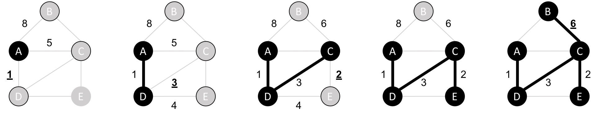
Figure 4-10. Minimum Spanning Tree algorithm steps
-
It begins with a tree containing only one node.
-
Then the relationship with smallest weight coming from that node is selected and added to the tree (along with its connected node).
-
This process is repeated, always choosing the minimal-weight relationship that joins any node not already in the tree
-
When there are no more nodes to add, the tree is a minimum spanning tree.
There are also variants of this algorithm that find the maximum weight spanning tree, where we find the highest cost tree, or k-spanning tree, where we limit the size of the resulting tree.
When should I use Minimum Spanning Tree?
Use Minimum Spanning Tree when you need the best route to visit all nodes. Because the route is chosen based on the cost of each next step, it’s useful when you must visit all nodes in a single walk. (Review the previous section on Single Source Shortest Path if you don’t need a path for a single trip.)
You can use this algorithm for optimizing paths for connected systems like water pipes and circuit design. It’s also employed to approximate some problems with unknown compute times such as the traveling salesman problem and certain types of rounding.
Example use cases include:
-
Minimizing the travel cost of exploring a country. “An Application of Minimum Spanning Trees to Travel Planning” 18 describes how the algorithm analyzed airline and sea connections to do this.
-
Visualizing correlations between currency returns. This is described in “Minimum Spanning Tree Application in the Currency Market” 19.
-
Tracing the history of infection transmission in an outbreak. For more information, see “Use of the Minimum Spanning Tree Model for Molecular Epidemiological Investigation of a Nosocomial Outbreak of Hepatitis C Virus Infection” 20.
Warning
The Minimum Spanning Tree algorithm only gives meaningful results when run on a graph where the relationships have different weights. If the graph has no weights, or all relationships have the same weight, then any spanning tree is a minimum spanning tree.
Minimum Spanning Tree with Neo4j
Let’s see the Minimum Spanning Tree algorithm in action. The following query finds a spanning tree starting from Amsterdam:
MATCH(n:Place {id:"Amsterdam"})CALL algo.spanningTree.minimum("Place","EROAD","distance",id(n),{write:true, writeProperty:"MINST"})YIELD loadMillis, computeMillis, writeMillis, effectiveNodeCountRETURNloadMillis, computeMillis, writeMillis, effectiveNodeCount
The parameters passed to this algorithm are:
-
Place-the node labels to consider when computing the spanning tree -
EROAD-the relationship types to consider when computing the spanning tree -
distance-the name of the relationship property that indicates the cost of traversing between a pair of nodes -
id(n)-the internal node id of the node from which the spanning tree should begin
This query stores its results in the graph. If we want to return the minimum weight spanning tree we can run the following query:
MATCHpath = (n:Place {id:"Amsterdam"})-[:MINST*]-()WITHrelationships(path)ASrelsUNWIND relsAS relWITH DISTINCT rel AS relRETURNstartNode(rel).idASsource, endNode(rel).idASdestination,rel.distanceAScost
And this is the output of the query:
| source | destination | cost |
|---|---|---|
Amsterdam |
Utrecht |
46.0 |
Utrecht |
Gouda |
35.0 |
Gouda |
Rotterdam |
25.0 |
Rotterdam |
Den Haag |
26.0 |
Den Haag |
Hoek van Holland |
27.0 |
Hoek van Holland |
Felixstowe |
207.0 |
Felixstowe |
Ipswich |
22.0 |
Ipswich |
Colchester |
32.0 |
Colchester |
London |
106.0 |
London |
Doncaster |
277.0 |
Doncaster |
Immingham |
74.0 |
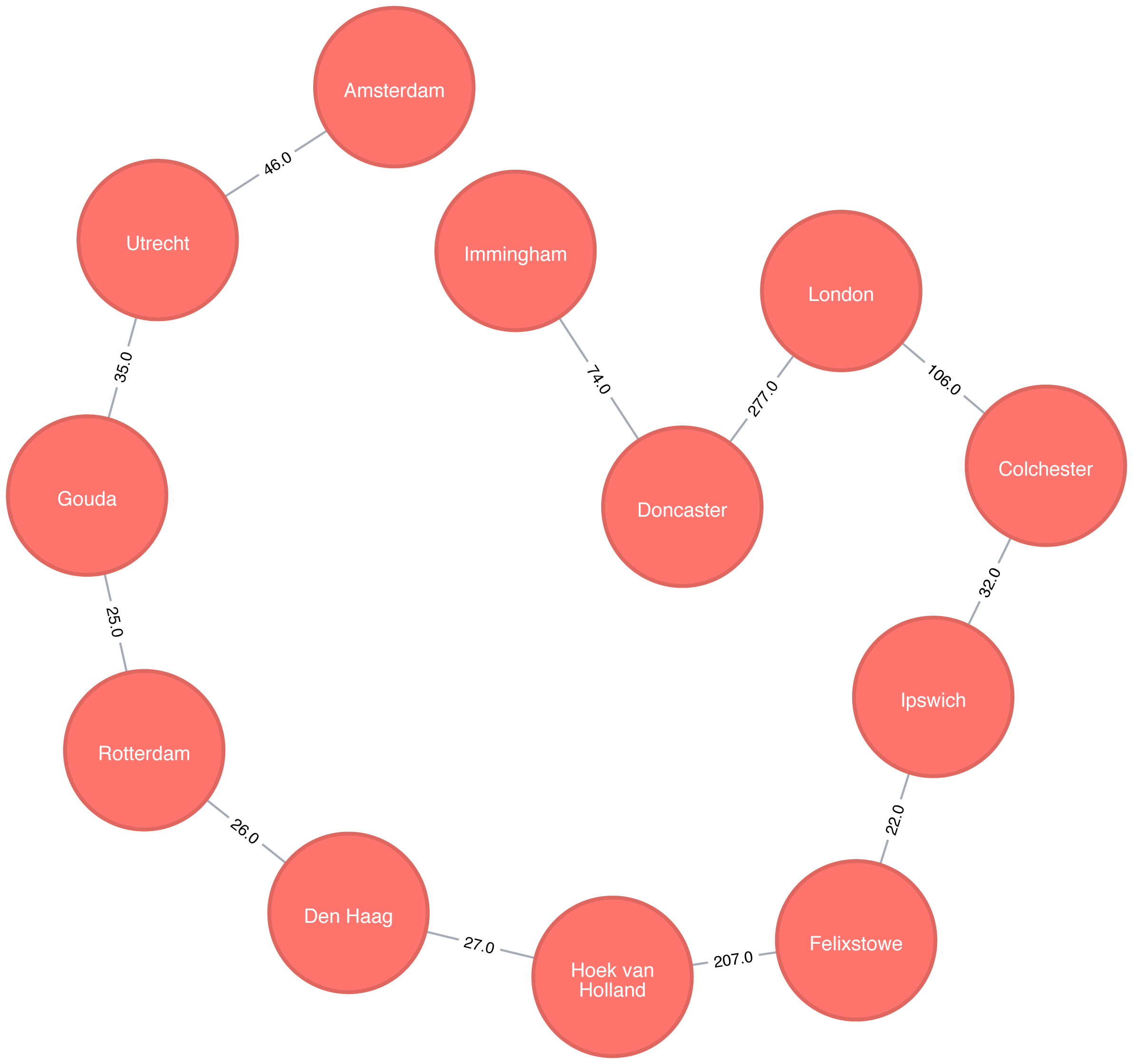
Figure 4-11. A minimum weight spanning tree from Amsterdam
If we were in Amsterdam and wanted to visit every other place in our dataset, Figure 4-11 demonstrates the shortest continuous route to do so.
Random Walk
The Random Walk algorithm that provides a set of nodes on a random path in a graph. The term was first mentioned by Karl Pearson in 1905 in a letter to Nature magazine titled “The Problem of the Random Walk” 21. Although the concept goes back even further, it’s only more recently that random walks have been applied to network science.
A random walk, in general, is sometimes described as being similar to how a drunk person traverses a city. They know what direction or end point they want to reach but may take a very circuitous route to get there.
The algorithm starts at one node and somewhat randomly follows one of the relationships forward or back to a neighbor node. It then does the same from that node and so on, until it reaches the set path length. (We say somewhat randomly because the number of relationships a node has, and its neighbors have, influences the probability a node will be walked through.)
When should I use Random Walk?
Use the Random Walk algorithm as part of other algorithms or data pipelines when you need to generate a mostly random set of connected nodes.
Example use cases include:
-
It can be used as part of the node2vec and graph2vec algorithms, that create node embeddings. These node embeddings could then be used as the input to a neural network.
-
It can be used as part of the Walktrap and Infomap community detection* algorithms. If a random walk returns a small set of nodes repeatedly, then it indicates that those set of nodes may have a community structure.
-
The training process of machine learning models. This is described further in David Mack’s article “Review Prediction with Neo4j and TensorFlow” 22.
You can read about more use cases in Random walks and diffusion on networks 23.
Random Walk with Neo4j
Neo4j has an implementation of the Random Walk algorithm. It supports two modes for choosing the next relationship to follow at each stage of the algorithm:
-
random-randomly chooses a relationship to follow -
node2vec-chooses relationship to follow based on computing a probability distribution of the previous neighbours
The following query does this:
MATCH(source:Place {id:"London"})CALL algo.randomWalk.stream(id(source), 5, 1)YIELD nodeIdsUNWIND algo.getNodesById(nodeIds)ASplaceRETURNplace.idASplace
The parameters passed to this algorithm are:
-
id(source)-the internal node id of the starting point for our random walk -
5-the number of hops our random walk should take -
1-the number of random walks we want to compute
It returns the following result:
| place |
|---|
London |
Doncaster |
Immingham |
Amsterdam |
Utrecht |
Amsterdam |
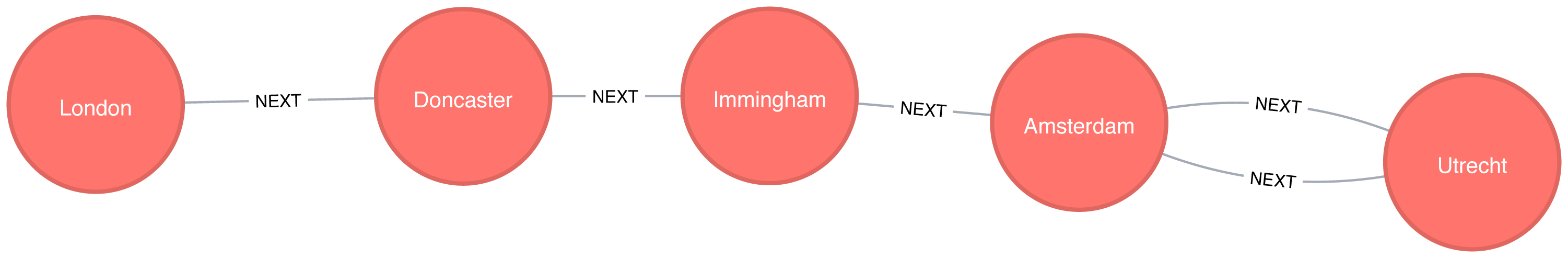
Figure 4-12. A random walk starting from London
At each stage of the random walk the next relationship to follow is chosen randomly. This means that if we run the alogrithm again, even with the same parameters, we likely won’t get the exact same result. It’s also possible for a walk to go back on itself as we can see in Figure 4-12 where we go from Amsterdam to Den Haag and back again.
Summary
Pathfinding algorithms are useful for understanding the way that our data is connected. In this chapter we started out with the fundamental Breadth- and Depth-First algorithms, before moving onto Dijkstra and other shortest path algorithms.
We’ve also learnt about variants of the shortest path algorithms that are optimised for finding the shortest path from one node to all other nodes or between all pairs of nodes in a graph. We finished by learning about the random walk algorithm which can be used to find arbitrary sets of paths.
Next we’ll learn about Centrality algorithms that can be used to find influential nodes in a graph.
1 http://www.elbruz.org/e-roads/
2 https://github.com/neo4j-graph-analytics/book/blob/master/data/transport-nodes.csv
3 https://github.com/neo4j-graph-analytics/book/blob/master/data/transport-relationships.csv
4 https://github.com/neo4j-graph-analytics/book
5 https://ieeexplore.ieee.org/document/5219222/?arnumber=5219222
7 https://www.oakland.edu/enp/
8 https://github.com/graphframes/graphframes/issues/185
9 https://graphframes.github.io/user-guide.html#message-passing-via-aggregatemessages
10 https://github.com/neo4j-graph-analytics/book/blob/master/scripts/aggregate_messages/aggregate_messages.py
11 https://ieeexplore.ieee.org/document/4082128/
12 https://pubsonline.informs.org/doi/abs/10.1287/mnsc.17.11.712
13 http://web.mit.edu/urban_or_book/www/book/
14 https://cs.uwaterloo.ca/research/tr/2011/CS-2011-21.pdf
15 https://routing-bits.com/2009/08/06/ospf-convergence/
16 https://en.wikipedia.org/wiki/Open_Shortest_Path_First
17 https://arxiv.org/pdf/1604.02113v1.pdf
18 http://www.dwu.ac.pg/en/images/Research_Journal/2010_Vol_12/1_Fitina_et_al_spanning_trees_for_travel_planning.pdf
19 https://www.nbs.sk/_img/Documents/_PUBLIK_NBS_FSR/Biatec/Rok2013/07-2013/05_biatec13-7_resovsky_EN.pdf
20 https://www.ncbi.nlm.nih.gov/pmc/articles/PMC516344/
21 https://www.nature.com/physics/looking-back/pearson/index.html
22 https://medium.com/octavian-ai/review-prediction-with-neo4j-and-tensorflow-1cd33996632a