Table of Contents for
Graph Algorithms
 Graph Algorithms
Published by
O'Reilly Media, Inc., 2019
Graph Algorithms
Published by
O'Reilly Media, Inc., 2019
- Cover
- nav
- Graph Algorithms
- Graph Algorithms
- Preface
- 1. Introduction
- 2. Graph Theory and Concepts
- 3. Graph Platforms and Processing
- 4. Pathfinding and Graph Search Algorithms
- 5. Centrality Algorithms
- 6. Community Detection Algorithms
- 7. Graph Algorithms in Practice
- 8. Using Graph Algorithms to Enhance Machine Learning
- About the Authors
Chapter 2. Graph Theory and Concepts
In this chapter, we go into more detail on the terminology of graph algorithms. The basics of graph theory are explained with a focus on the concepts that are most relevant to a practitioner.
We’ll describe how graphs are represented and then explain the different types of graphs and their attributes. This will be important later as our graph’s characteristics will inform our algorithm choices and help interpret results. We’ll finish the chapter with the types of graph algorithms available to us.
Terminology
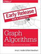
The labeled property graph is the dominant way of modeling graph data. An example can be seen in Figure 2-1.
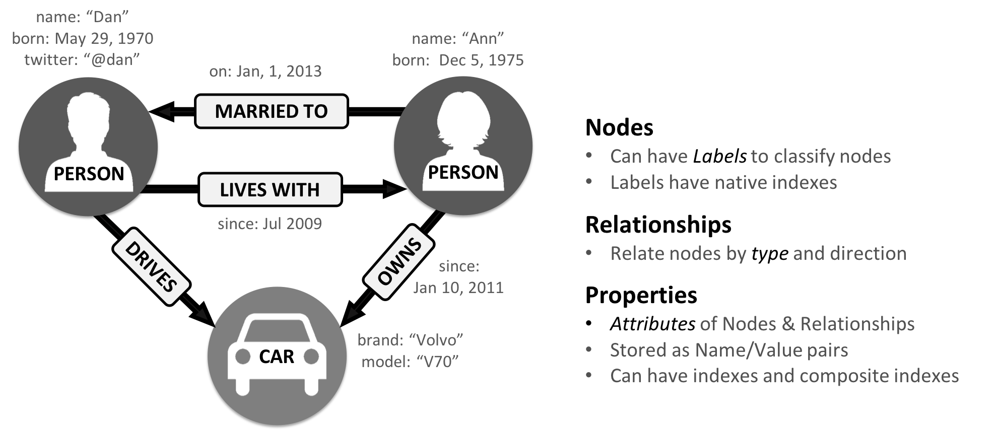
Figure 2-1. Labeled Property Graph Model
A label marks a node as part of a group. Here we have two groups of nodes: Person and Car. (Although in classic graph theory, a label applies to a single node, it’s now commonly used to mean a node group.)
Relationships are classified based on relationship-type. Our example includes the relationship types of DRIVES, OWNS, LIVES_WITH, and MARRIED_TO.
Properties are synonymous with attributes and can contain a variety of data types from numbers and strings to spatial and temporal data. In Figure 2-1 , we assigned the properties as named value pairs where the name of the property comes first and then its value. For example, the Person node on the left has a property name: Dan and the MARRIED_TO relationship as a property of on: Jan, 1, 2013 .
A subgraph is a graph within a larger graph. Subgraphs are useful as a filter for our graph such as when we need a subset with particular characteristics for focused analysis.
A path is a group of nodes and their connecting relationships. An example of a simple path, based on Figure 2-1, could contain the nodes Dan, Ann and Car and the LIVES_WITH and OWNS relationships.
Graphs vary in type, shape and size as well the kind of attributes that can be used for analysis. In the next section, we’ll describe the kinds of graphs most suited for graph algorithms. Keep in mind that these explanations apply to graphs as well as subgraphs.
Basic Graph Types and Structures
In classic graph theory, the term graph is equated with a simple (or strict) graph where nodes only have one relationship between them, as shown on the left side of Figure 2-2. Most real-world graphs, however, has many relationships between nodes and even self-referencing relationships. Today, the term graph is commonly used for all three graph types in Figure 2-2 and so we also use the term inclusively.

Figure 2-2. In this book, we use the term “graph” to include any of these classic types of graphs.
Random, Small-World, Scale-Free Structures
Graphs take on a variety of shapes. Figure 2-3 illustrates three representative network types:
- random networks
- small-world networks
- scale-free networks
These network types produce graphs with distinctive structures, distributions, and behaviors.
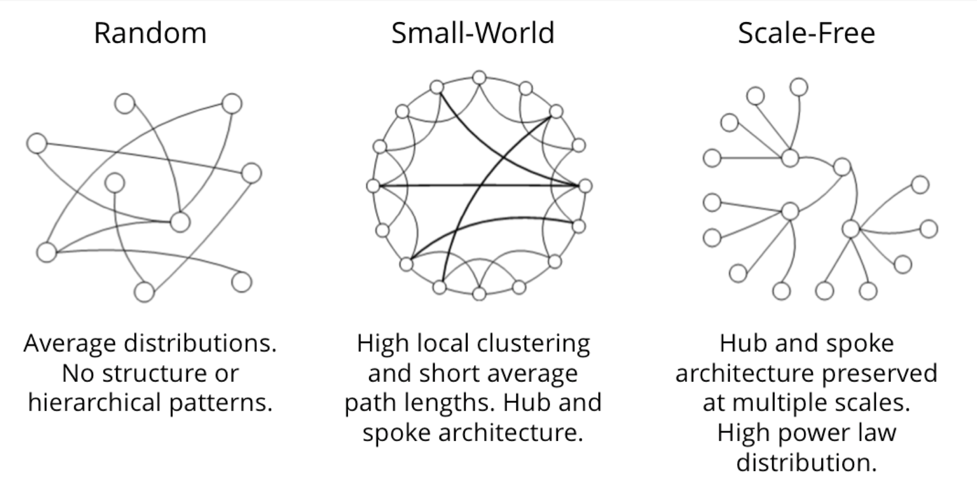
Figure 2-3. Three network structures with distinctive graphs and behavior.
- In a completely average distribution of connections, a random network is formed with no hierarchies. This type of shapeless graph is “flat” with no discernible patterns. All nodes have the same probability of being attached to any other node.
- A small-world network is extremely common in social networks and shows localized connections and some hub-spoke pattern. The "Six Degrees of Kevin Bacon" game might be the best-known example of the small-world effect. Although you associate mostly with a small group of friends, you’re never many hops away from anyone else—even if they are a famous actor or on the other side of the planet.
- A scale-free network is produced when there are power-law distributions and a hub and spoke architecture is preserved regardless of scale, such as the World Wide Web.
Flavors of Graphs
To get the most out of graph algorithms, it’s important to familiarize ourselves with the most characteristic graphs we’ll encounter.
| Graph Attributes | Key Factor | Algorithm Consideration |
|---|---|---|
| Connected versus Disconnected | Whether or not there is a path between any two nodes in the graph, irrespective of distance. | Islands of nodes can cause unexpected behavior such as getting stuck in or failing to process disconnected components. |
| Weighted versus Unweighted | Whether there are (domain-specific) values on relationships or nodes. | Many algorithms expect weights and we’ll see significant differences in performance and results when ignored. |
| Directed versus Undirected | Whether or not relationships explicitly define a start and end node. |
Adds rich context to infer additional meaning. In some algorithms, you can explicitly set the use of one, both, or no direction. |
| Cyclic versus Acyclic | Paths start and end at the same node | Cyclic is common but algorithms must be careful (typically by storing traversal state) or cycles may prevent termination. Acyclic graphs (or spanning trees) are the basis for many graph algorithms. |
| Sparse versus Dense | Relationship to node ratio | Extremely dense or extremely sparsely connected graphs can cause divergent results. Data modeling may help, assuming the domain is not inherently dense or sparse. |
| Monopartite, Bipartite, and K-Partite | Nodes connect to only one other node type (users like movies) versus many other node types (users like users who like movies) | Helpful for creating relationships to analyze and projecting more useful graphs. |
Connected versus Disconnected Graphs
A graph is connected if there is a path from any node to every node and disconnected if there is not. If we have islands in our graph, it’s disconnected. If the nodes in those islands are connected, they are called components (or sometimes clusters) as shown in Figure 2-4.

Figure 2-4. If we have islands in our graph, it’s a disconnected graph.
Some algorithms struggle with disconnected graphs and can produce misleading results. If we have unexpected results, checking the structure of our graph is a good first step.
Unweighted Graphs versus Weighted Graphs
Unweighted graphs have no weight values assigned to their nodes or relationships. For weighted graphs, these values can represent a variety of measures such as cost, time, distance, capacity, or even a domain-specific prioritization. Figure 2-5 visualizes the difference.
Figure 2-5. Weighted graphs can hold values on relationships or nodes.
Basic graph algorithms can use weights for processing as a representation for the strength or value of relationships. Many algorithms compute metrics which then can be used as weights for follow-up processing. Some algorithms update weight values as they proceed to find cumulative totals, lowest values, or optimums.
The classic use for weighted graphs is in pathfinding algorithms. Such algorithms underpin the mapping applications on our phones and compute the shortest/cheapest/fastest transport routes between locations. For example, Figure 2-6 uses two different methods of computing the shortest route.
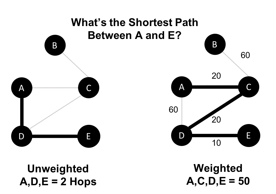
Figure 2-6. The shortest paths can vary for an otherwise identical unweighted and weighted graph.
Without weights, our shortest route is calculated in terms of the number of relationships (commonly called hops). A and E have a 2 hop shortest path, which indicates only 1 city (D) between them. However, the shortest weighted path from A to E takes us from A to C to D to E. If weights represent a physical distance in kilometers the total distance would be 50 km. In this case, the shortest path in terms of the number of hops would equate to a longer physical route of 70 km.
Undirected Graphs versus Directed Graphs
In an undirected graph, relationships are considered bi-directional, such as commonly used for friendships. In a directed graph, relationships have a specific direction. Relationships pointing to a node are referred to as in-links and, unsurprisingly, out-links are those originating from a node.
Direction adds another dimension of information. Relationships of the same type but in opposing directions carry different semantic meaning, as it expresses a dependency or indicates a flow. This may then be used as an indicator of credibility or group strength. Personal preferences and social relations are expressed very well with direction.
For example, if we assumed in Figure 2-7 that the directed graph was a network of students and the relationships were “likes” then we’d calculate that A and C are more popular.
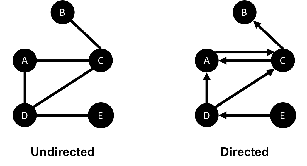
Figure 2-7. Many algorithms allow us to compute on the basis of only inbound or outbound connections, both directions, or without direction.
Road networks illustrate why we might want to use both types of graphs. For example, highways between cities are often traveled in both directions. However, within cities, some roads are one-way streets. (The same is true for some information flows!)
We get different results running algorithms in an undirected fashion compared to directed. If we want an undirected graph, for example, we would assume highways or friendship always go both ways.
If we reimagine Figure 2-7 as a directed road network, you can drive to A from C and D but you can only leave through C. Furthermore if there were no relationships from A to C, that would indicate a dead-end. Perhaps that’s less likely for a one-way road network but not for a process or a webpage.
Acyclic Graphs versus Cyclic Graphs
In graph theory, cycles are paths through relationships and nodes which start and end at the same node. An acyclic graph has no such cycles. As shown in Figure 2-8, directed and undirected graphs can have cycles but when directed, paths follow the relationship direction. A directed acyclic graph (DAG), shown in Graph 1, will by definition always have dead ends (leaf nodes).
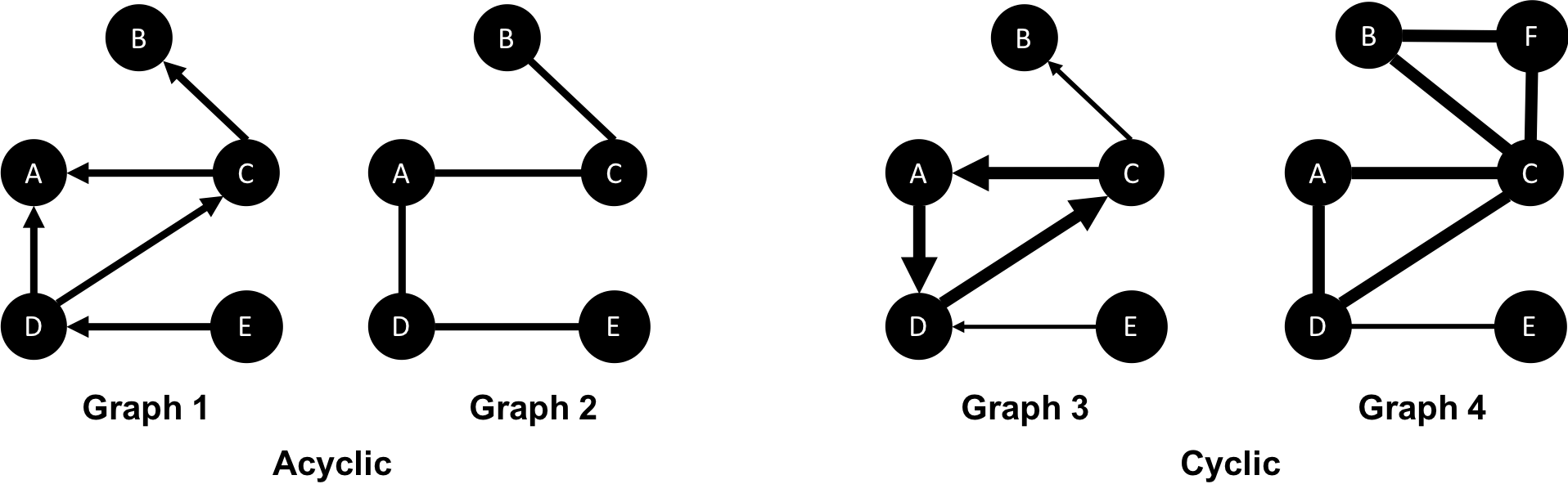
Figure 2-8. In acyclic graphs, it’s impossible to start and end on the same node without retracing our steps.
Graphs 1 and 2 have no cycles as there’s no way to start and end on the same node without repeating a relationship. You might remember from chapter 1 that not repeating relationships was the Königsberg bridges problem that started graph theory! Graph 3 in Figure 2-8 shows a simple cycle with no repeated nodes of A-D-C-A. In graph 4, the undirected cyclic graph has been made more interesting by adding a node and relationship. There’s now a closed cycle with a repeated node (C), following B-F-C-D-A-C-B. There are actually multiple cycles in graph 4.
Cycles are common and we sometimes need to convert cyclic graphs to acyclic graphs (by cutting relationships) to eliminate processing problems. Directed acyclic graphs naturally arise in scheduling, genealogy, and version histories.
Trees
In classic graph theory, an acyclic graph that is undirected is called a tree. While, in computer science, trees can also be directed. A more inclusive definition would be a graph where any two nodes are connected by only one path. Trees are significant for understanding graph structures and many algorithms. They play a key role in designing networks, data structures, and search optimizations to improve categorization or organizational hierarchies.
Much has been written about trees and their variations, Figure 2-9 illustrates the common trees that we’re likely to encounter.
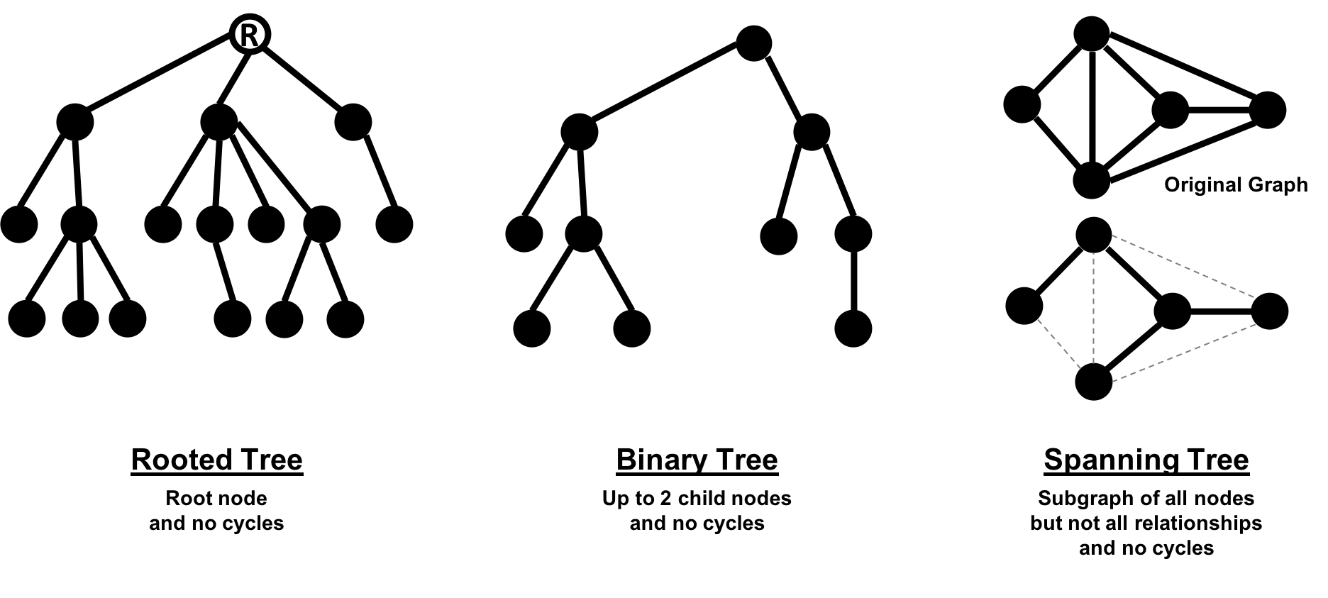
Figure 2-9. Of these prototypical tree graphs, spanning trees are most often used for graph algorithms.
Of these variations, spanning trees are the most relevant for this book. A spanning tree is a subgraph, that includes all the nodes of a larger acyclic graph but not all the relationships. A minimum spanning tree connects all the nodes of a graph with the either the least number of hops or least weighted paths.
Sparse Graphs versus Dense Graphs
The sparsity of a graph is based on the number of relationships it has compared to the maximum possible number of relationships, which would occur if there was a relationship between every pair of nodes. A graph where every node has a relationship with every other node is called a complete graph, or a clique for components. For instance, if all my friends knew each other, that would be a clique.
The maximum density of a graph is calculated with the formula,[ where N is the number of nodes. Any graph that approaches the maximum density is considered dense, although there is no strict definition. In Figure 2-10 we can see three measures of density for undirected graphs which uses the formula, where R is the number of relationships.
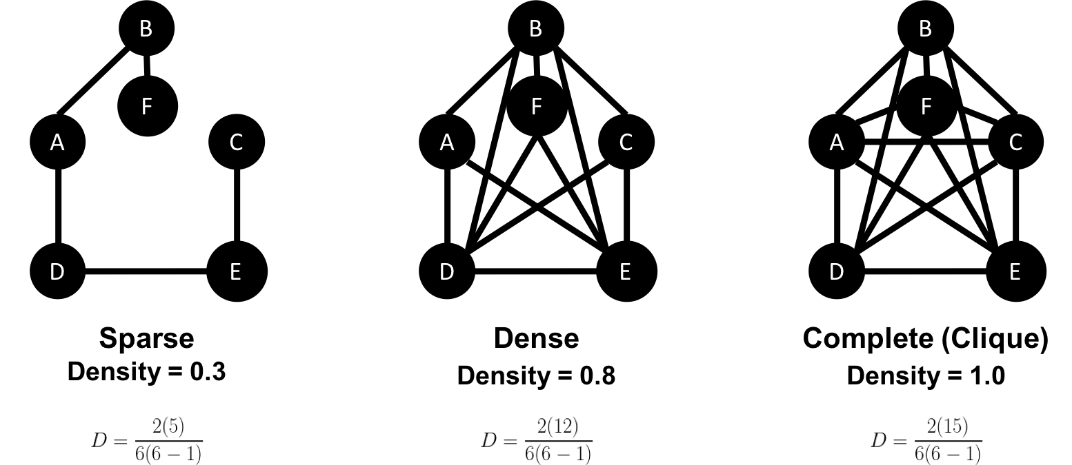
Figure 2-10. Checking the density of a graph can help evaluate unexpected results.
Most graphs based on real networks tend toward sparseness with an approximately linear correlation of total nodes to total relationships. This is especially the case where physical elements come into play such as the practical limitations to how many wires, pipes, roads, or friendships you can join at one point.
Some algorithms will return nonsensical results when executed on very sparse or dense graphs. If a graph is very sparse there may not be enough relationships for algorithms to compute useful results. Alternatively, very densely connected nodes don’t add much additional information since they are so highly connected. Dense nodes may also skew some results or add computational complexity.
Monopartite, Bipartite, and K-Partite Graphs
Most networks contain data with multiple node and relationship types. Graph algorithms, however, frequently consider only one node type and one relationship type. Graphs with one one node type and relationship type are sometimes referred to as monopartite
A bipartite graph is a graph whose nodes can be divided into two sets, such that relationships only connect a node from one set to a node from a different set. Figure 2-11 shows an example of such a graph. It has 2 sets of nodes: a viewer set and a TV-show set. There are only relationships between the two sets and no intra-set connections. In other words in Graph 1, TV shows are only related to viewers, not other TV shows and viewers are likewise not directly linked to other viewers.
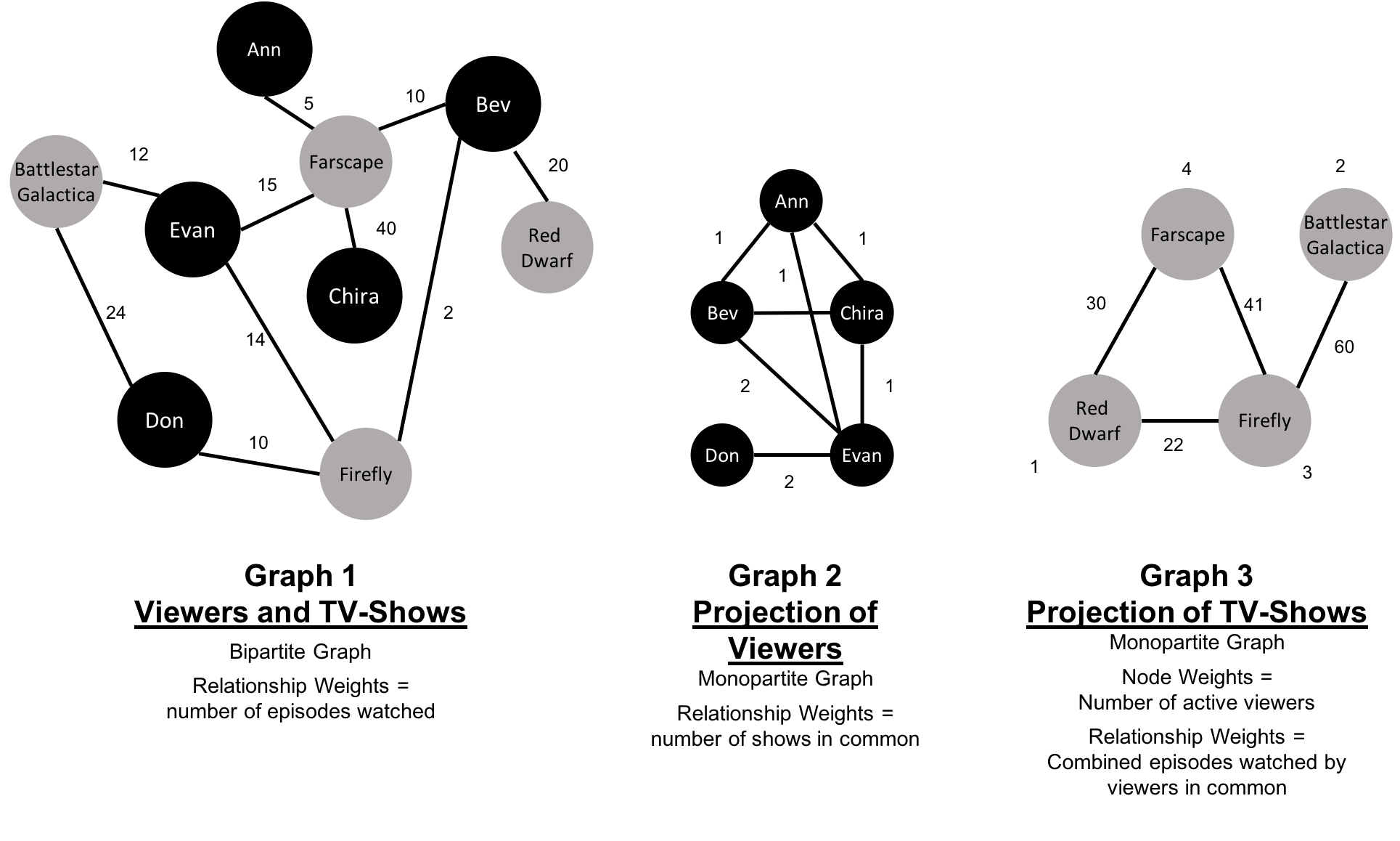
Figure 2-11. Bipartite graphs are often projected to monopartite graphs for more specific analysis.
Starting from our bipartite graph of viewers and TV-shows we created two monopartite projections: Graph 2 of viewer connections based on movies in common and Graph 3 of TV shows based on viewers in common. We can also filter based on relationship type such as watched, rated, or reviewed.
Projecting monopartite graphs with inferred connections is an important part of graph analysis. These type of projections help uncover indirect relationships and qualities. For example, in Figure 2-11 Graph 2, we’ve weighted relationship in the TV show graph by the aggregated views by viewers common. In this case, Bev and Ann have watched only one TV show in common whereas Bev and Evan have two shows in common. This, or other metrics such as similarity, can be used to infer meaning between activities like watching Battlestar Galactica and Firefly. That can inform our recommendation for someone similar to Evan who, in Figure 2-11, just finished watching the last episode of Firefly.
K-partite graphs reference the number of node-types our data has (k). For example, if we have 3 node types, we’d have a tripartite graph. This just extends bipartite and monopartite concepts to account for more node types. Many real-world graphs, especially knowledge graphs, have a large value for k, as they combine many different concepts and types of information. An example of using a larger number of node-types is creating new recipes by mapping a recipe set to an ingredient set to a chemical compound—and then deducing new mixes that connect popular preferences. We could also reduce the number of nodes-types by generalization such as treating many forms of a node, like spinach or collards, as just as a “leafy green.”
Now that we’ve reviewed the types of graphs we’re most likely to work with, let’s learn about the types of graph algorithms we can execute on those graphs.
Types of Graph Algorithms
Let’s look into the three areas of analysis that are at the heart of graph algorithms. These categories correspond to the chapters on algorithms for pathfinding and search, centrality computation and community detection.
Pathfinding
Paths are fundamental to graph analytics and algorithms. Finding shortest paths is probably the most frequent task performed with graph algorithms and is a precursor for several different types of analysis. The shortest path is the traversal route with the fewest hops or lowest weight. If the graph is directed, then it’s the shortest path between two nodes as allowed by the relationship directions.
Centrality
Centrality is all about understanding which nodes are more important in a network. But what do we mean by importance? There are different types of centrality algorithms created to measure different things such as the ability to quickly spread information versus bridge between distinct groups. In this book, we are mostly focused on topological analysis: looking at how nodes and relationships are structured.
Community Detection
Connectedness is a core concept of graph theory that enables a sophisticated network analysis such as finding communities. Most real-world networks exhibit sub-structures (often quasi-fractal) of more or less independent subgraphs.
Connectivity is used to find communities and quantify the quality of groupings. Evaluating different types of communities within a graph can uncover structures, like hubs and hierarchies, and tendencies of groups to attract or repel others. These techniques are used to study the phenomenon in modern social networks that lead to echo chambers and filter-bubble effects, which are prevalent in modern political science.
Summary
Graphs are intuitive. They align with how we think about and draw systems. The primary tenets of working with graphs can be quickly assimilated once we’ve unraveled some of the terminology and layers. In this chapter we’ve explained the ideas and expressions used later in this book and described flavors of graphs you’ll come across.
Next, we’ll look at graph processing and types of analysis before diving into how to use graph algorithms in Apache Spark and Neo4j.