Table of Contents for
Graph Algorithms
 Graph Algorithms
Published by
O'Reilly Media, Inc., 2019
Graph Algorithms
Published by
O'Reilly Media, Inc., 2019
- Cover
- nav
- Graph Algorithms
- Graph Algorithms
- Preface
- 1. Introduction
- 2. Graph Theory and Concepts
- 3. Graph Platforms and Processing
- 4. Pathfinding and Graph Search Algorithms
- 5. Centrality Algorithms
- 6. Community Detection Algorithms
- 7. Graph Algorithms in Practice
- 8. Using Graph Algorithms to Enhance Machine Learning
- About the Authors
Chapter 5. Centrality Algorithms
Centrality algorithms are used to understand the roles of particular nodes in a graph and their impact on that network. Centrality algorithms are useful because they identify the most important nodes and help us understand group dynamics such as credibility, accessibility, the speed at which things spread, and bridges between groups. Although many of these algorithms were invented for social network analysis, they have since found uses in many industries and fields.
We’ll cover the following algorithms:
-
Degree Centrality as a baseline metric of connectedness
-
Closeness Centrality for measuring how central a node is to the group, including two variations for disconnected groups
-
Betweenness Centrality for finding control points, including an alternative for approximation
-
PageRank for understanding the overall influence, including a popular option for personalization
Tip
Different centrality algorithms can produce significantly different results based on what they were created to measure. When we see sub-optimal answers, it’s best to check our algorithm use is in alignment with its intended purpose.
We’ll explain how these algorithms work and show examples in Spark and Neo4j. Where an algorithm is unavailable on one platform or where the differences are unimportant, we’ll provide just one platform example.
| Algorithm Type | What It Does | Example Uses | Spark Example | Neo4j Example |
|---|---|---|---|---|
Measures the number of relationships a node has. |
Estimate a person’s popularity by looking at their in-degree and use their out-degree for gregariousness. |
Yes |
No |
|
Variations: Wasserman and Faust, Harmonic Centrality |
Calculates which nodes have the shortest paths to all other nodes. |
Find the optimal location of new public services for maximum accessibility. |
Yes |
Yes |
Measures the number of shortest paths that pass through a node. |
Improve drug targeting by finding the control genes for specific diseases. |
No |
Yes |
|
Variation: Personalized PageRank |
Estimates a current node’s importance from its linked neighbors and their neighbors. Popularized by Google. |
Find the most influential features for extraction in machine learning and rank text for entity relevance in natural language processing. |
Yes |
Yes |
Figure 5-1 illustrates the graph that we want to construct:
We have one larger set of users with connections between them and a smaller set with no connections to that larger group.
Let’s create graphs in Apache Spark and Neo4j based on the contents of those CSV files.
Importing the data into Apache Spark
First, we’ll import the required packages from Apache Spark and the GraphFrames package.
fromgraphframesimport*frompysparkimportSparkContext
We can write the following code to create a GraphFrame based on the contents of the above CSV files.
v=spark.read.csv("data/social-nodes.csv",header=True)e=spark.read.csv("data/social-relationships.csv",header=True)g=GraphFrame(v,e)
Importing the data into Neo4j
Next, we’ll load the data for Neo4j. The following query imports nodes:
WITH"https://github.com/neo4j-graph-analytics/book/raw/master/data/social-nodes.csv"ASuriLOAD CSVWITHHEADERS FROM uriASrowMERGE (:User {id: row.id})
And this query imports relationships:
WITH"https://github.com/neo4j-graph-analytics/book/raw/master/data/social-relationships.csv"ASuriLOAD CSVWITHHEADERS FROM uriASrowMATCH(source:User {id: row.src})MATCH(destination:User {id: row.dst})MERGE (source)-[:FOLLOWS]->(destination)
Now that our graphs are loaded, it’s onto the algorithms!
Degree Centrality
Degree Centrality is the simplest of the algorithms that we’ll cover in this book. It counts the number of incoming and outgoing relationships from a node, and is used to find popular nodes in a graph.
Degree Centrality was proposed by Linton C. Freeman in his 1979 paper Centrality in Social Networks Conceptual Clarification 1.
Reach
Understanding the reach of a node is a fair measure of importance. How many other nodes can it touch right now? The degree of a node is the number of direct relationships it has, calculated for in- degree and out-degree. You can think of this as the immediate reach of node. For example, a person with a high degree in an active social network would have a lot of immediate contacts and be more likely to catch a cold circulating in their network.
The average degree of a network is simply the total number of relationships divided by the total number of nodes; it can be heavily skewed by high degree nodes. Alternatively, the degree distribution is the probability that a randomly selected node will have a certain number of relationships.
Figure 5-2 illustrates the difference looking at the actual distribution of connections among subreddit topics. If you simply took the average, you’d assume most topics have 10 connections whereas, in fact, most topics only have 2 connections.
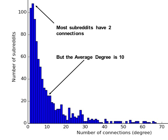
Figure 5-2. Mapping of subreddit degree distribution by Jacob Silterra provides an example of how the average does not often reflect the actual distribution in networks
These measures are used to categorize network types such as the scale-free or small-world networks that were discussed in chapter 2. They also provide a quick measure to help estimate the potential for things to spread or ripple throughout a network.
When Should I Use Degree Centrality?
Use Degree Centrality if you’re attempting to analyze influence by looking at the number of incoming and outgoing relationships, or find the “popularity” of individual nodes. It works well when you’re concerned with immediate connectedness or near-term probabilities. However, Degree Centrality is also applied to global analysis when you want to evaluate the minimum degree, maximum degree, mean degree, and standard deviation across the entire graph.
Example use cases include:
-
Degree Centrality is used to identify powerful individuals though their relationships, such as connections of people on a social network. For example, in BrandWatch’s most influential men and women on Twitter 2017 2, the top five people in each category have over 40 million followers each.
-
Weighted Degree Centrality has been applied to help separate fraudsters from legitimate users of an online auction. The weighted centrality of fraudsters tends to be significantly higher due collusion aimed at artificially increasing prices. Read more in Two Step graph-based semi-supervised Learning for Online Auction Fraud Detection. 3
Degree Centrality with Apache Spark
Now we’ll execute the Degree Centrality algorithm with the following code:
total_degree=g.degreesin_degree=g.inDegreesout_degree=g.outDegreestotal_degree.join(in_degree,"id",how="left")\.join(out_degree,"id",how="left")\.fillna(0)\.sort("inDegree",ascending=False)\.show()
We first calculated the total, in, and out degrees. Then we joined those DataFrames together, using a left join to retain any nodes that don’t have incoming or outgoing relationships.
If nodes don’t have relationships we set that value to 0 using the fillna function.
Let’s run the code in pyspark:
| id | degree | inDegree | outDegree |
|---|---|---|---|
Doug |
6 |
5 |
1 |
Alice |
7 |
3 |
4 |
Michael |
5 |
2 |
3 |
Bridget |
5 |
2 |
3 |
Charles |
2 |
1 |
1 |
Mark |
3 |
1 |
2 |
David |
2 |
1 |
1 |
Amy |
1 |
1 |
0 |
James |
1 |
0 |
1 |
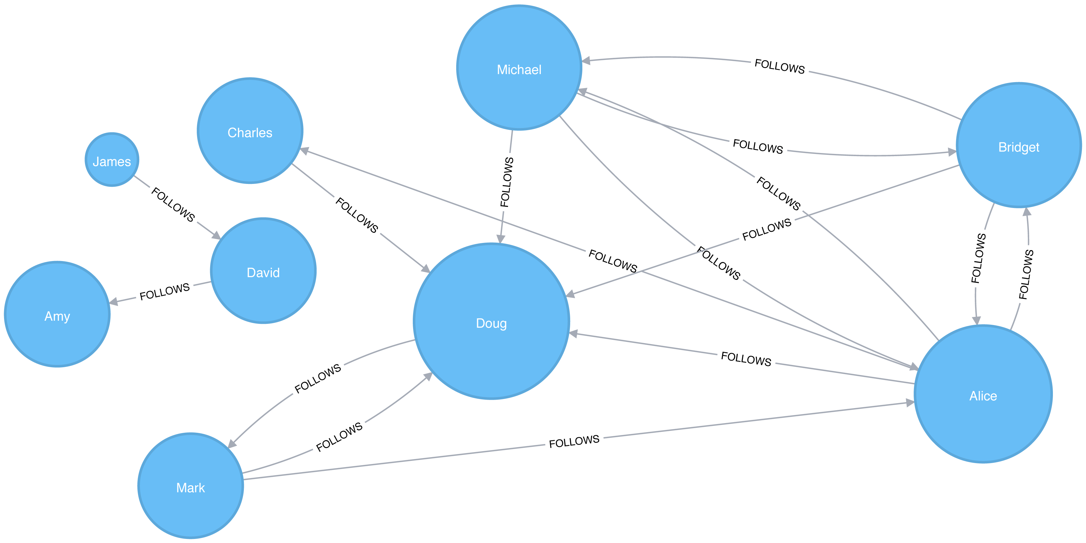
Figure 5-3. Visualization of Degree Centrality
We can see in Figure 5-3 that Doug is the most popular user in our Twitter graph with five followers (in-links). All other users in that part of the graph follow him and he only follows one person back. In the real Twitter network, celebrities have high follower counts but tend to follow few people. We could therefore consider Doug a celebrity!
If we were creating a page showing the most followed users or wanted to suggest people to follow we would use this algorithm to identify those people.
Tip
Some data may contain very dense nodes with lots of relationships. These don’t add much additional information and can skew some results or add computational complexity. We may want to filter them with a subgraph or project the graph summarizes the relationships as a weight.
Closeness Centrality
Closeness Centrality is a way of detecting nodes that are able to spread information efficiently through a subgraph.
The closeness centrality of a node measures its average farness (inverse distance) to all other nodes. Nodes with a high closeness score have the shortest distances to all other nodes.
For each node, the Closeness Centrality algorithm calculates the sum of its distances to all other nodes, based on calculating the shortest paths between all pairs of nodes. The resulting sum is then inverted to determine the closeness centrality score for that node.
The closeness centrality of a node is calculated using the formula:
where:
-
uis a node -
nis the number of nodes in the graph -
d(u,v)is the shortest-path distance between another nodevandu
It is more common to normalize this score so that it represents the average length of the shortest paths rather than their sum. This adjustment allows comparisons of the closeness centrality of nodes of graphs of different sizes.
The formula for normalized closeness centrality is as follows:
When Should I Use Closeness Centrality?
Apply Closeness Centrality when you need to know which nodes disseminate things the fastest. Using weighted relationships can be especially helpful in evaluating interaction speeds in communication and behavioural analyses.
Example use cases include:
-
Closeness Centrality is used to uncover individuals in very favorable positions to control and acquire vital information and resources within an organization. One such study is Mapping Networks of Terrorist Cells 4 by Valdis E. Krebs.
-
Closeness Centrality is applied as a heuristic for estimating arrival time in telecommunications and package delivery where content flows through shortest paths to a predefined target. It is also used to shed light on propagation through all shortest paths simultaneously, such as infections spreading through a local community. Find more details in Centrality and Network Flow 5 by Stephen P. Borgatti.
-
Closeness Centrality also identifies the importance of words in a document, based on a graph-based keyphrase extraction process. This process is described by Florian Boudin in A Comparison of Centrality Measures for Graph-Based Keyphrase Extraction. 6
Warning
Closeness Centrality works best on connected graphs. When the original formula is applied to an unconnected graph, we end up with an infinite distance between two nodes where there is no path between them. This means that we’ll end up with an infinite closeness centrality score when we sum up all the distances from that node. To avoid this issue, a variation on the original formula will be shown after the next example.
Closeness Centrality with Apache Spark
Apache Spark doesn’t have a built in algorithm for Closeness Centrality, but we can write our own using the aggregateMessages framework that we introduced in the shortest weighted path section in the previous chapter.
Before we create our function, we’ll import some libraries that we’ll use:
fromscripts.aggregate_messagesimportAggregateMessagesasAMfrompyspark.sqlimportfunctionsasFfrompyspark.sql.typesimport*fromoperatorimportitemgetter
We’ll also create a few User Defined functions that we’ll need later:
defcollect_paths(paths):returnF.collect_set(paths)collect_paths_udf=F.udf(collect_paths,ArrayType(StringType()))paths_type=ArrayType(StructType([StructField("id",StringType()),StructField("distance",IntegerType())]))defflatten(ids):flat_list=[itemforsublistinidsforiteminsublist]returnlist(dict(sorted(flat_list,key=itemgetter(0))).items())flatten_udf=F.udf(flatten,paths_type)defnew_paths(paths,id):paths=[{"id":col1,"distance":col2+1}forcol1,col2inpathsifcol1!=id]paths.append({"id":id,"distance":1})returnpathsnew_paths_udf=F.udf(new_paths,paths_type)defmerge_paths(ids,new_ids,id):joined_ids=ids+(new_idsifnew_idselse[])merged_ids=[(col1,col2)forcol1,col2injoined_idsifcol1!=id]best_ids=dict(sorted(merged_ids,key=itemgetter(1),reverse=True))return[{"id":col1,"distance":col2}forcol1,col2inbest_ids.items()]merge_paths_udf=F.udf(merge_paths,paths_type)defcalculate_closeness(ids):nodes=len(ids)total_distance=sum([col2forcol1,col2inids])return0iftotal_distance==0elsenodes*1.0/total_distancecloseness_udf=F.udf(calculate_closeness,DoubleType())
And now for the main body that calculates the closeness centrality for each node:
vertices=g.vertices.withColumn("ids",F.array())cached_vertices=AM.getCachedDataFrame(vertices)g2=GraphFrame(cached_vertices,g.edges)foriinrange(0,g2.vertices.count()):msg_dst=new_paths_udf(AM.src["ids"],AM.src["id"])msg_src=new_paths_udf(AM.dst["ids"],AM.dst["id"])agg=g2.aggregateMessages(F.collect_set(AM.msg).alias("agg"),sendToSrc=msg_src,sendToDst=msg_dst)res=agg.withColumn("newIds",flatten_udf("agg")).drop("agg")new_vertices=g2.vertices.join(res,on="id",how="left_outer")\.withColumn("mergedIds",merge_paths_udf("ids","newIds","id"))\.drop("ids","newIds")\.withColumnRenamed("mergedIds","ids")cached_new_vertices=AM.getCachedDataFrame(new_vertices)g2=GraphFrame(cached_new_vertices,g2.edges)g2.vertices\.withColumn("closeness",closeness_udf("ids"))\.sort("closeness",ascending=False)\.show(truncate=False)
If we run that we’ll see the following output:
| id | ids | closeness |
|---|---|---|
Doug |
[[Charles, 1], [Mark, 1], [Alice, 1], [Bridget, 1], [Michael, 1]] |
1.0 |
Alice |
[[Charles, 1], [Mark, 1], [Bridget, 1], [Doug, 1], [Michael, 1]] |
1.0 |
David |
[[James, 1], [Amy, 1]] |
1.0 |
Bridget |
[[Charles, 2], [Mark, 2], [Alice, 1], [Doug, 1], [Michael, 1]] |
0.7142857142857143 |
Michael |
[[Charles, 2], [Mark, 2], [Alice, 1], [Doug, 1], [Bridget, 1]] |
0.7142857142857143 |
James |
[[Amy, 2], [David, 1]] |
0.6666666666666666 |
Amy |
[[James, 2], [David, 1]] |
0.6666666666666666 |
Mark |
[[Bridget, 2], [Charles, 2], [Michael, 2], [Doug, 1], [Alice, 1]] |
0.625 |
Charles |
[[Bridget, 2], [Mark, 2], [Michael, 2], [Doug, 1], [Alice, 1]] |
0.625 |
Alice, Doug, and David are the most closely connected nodes in the graph with a 1.0 score, which means each directly connects to all nodes in their part of the graph. Figure 5-4 illustrates that even though David has only a few connections, that’s significant within group of friends. In other words, this score represents their closeness to others within their subgraph but not the entire graph.
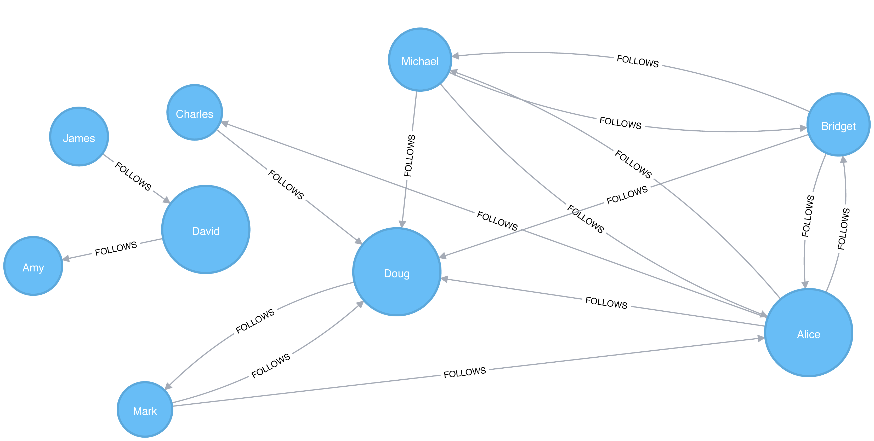
Figure 5-4. Visualization of Closeness Centrality
Closeness Centrality with Neo4j
Neo4j’s implementation of Closeness Centrality uses the following formula:
where:
-
uis a node -
nis the number of nodes in the same component (subgraph or group) asu -
d(u,v)is the shortest-path distance between another nodevandu
A call to the following procedure will calculate the closeness centrality for each of the nodes in our graph:
CALL algo.closeness.stream("User","FOLLOWS")YIELD nodeId, centralityRETURNalgo.getNodeById(nodeId).id, centralityORDER BYcentralityDESC
Running this procedure gives the following result:
| user | centrality |
|---|---|
Alice |
1.0 |
Doug |
1.0 |
David |
1.0 |
Bridget |
0.7142857142857143 |
Michael |
0.7142857142857143 |
Amy |
0.6666666666666666 |
James |
0.6666666666666666 |
Charles |
0.625 |
Mark |
0.625 |
We get the same results as with the Apache Spark algorithm but, as before, the score represents their closeness to others within their subgraph but not the entire graph.
Note
In the strict interpretation of the Closeness Centrality algorithm all the nodes in our graph would have a score of ∞ because every node has at least one other node that it’s unable to reach.
Ideally we’d like to get an indication of closeness across the whole graph, and in the next two sections we’ll learn about a few variations of the Closeness Centrality algorithm that do this.
Closeness Centrality Variation: Wasserman and Faust
Stanley Wasserman and Katherine Faust came up with 7 an improved formula for calculating closeness for graphs with multiple subgraphs without connections between those groups. The result of this formula is a ratio of the fraction of nodes in the group that are reachable, to the average distance from the reachable nodes.
The formula is as follows:
where:
-
uis a node -
Nis the total node count -
nis the number of nodes in the same component asu -
d(u,v)is the shortest-path distance between another nodevandu
We can tell the Closeness Centrality procedure to use this formula by passing the parameter improved: true.
The following query executes Closeness Centrality using the Wasserman Faust formula:
CALL algo.closeness.stream("User","FOLLOWS", {improved:true})YIELD nodeId, centralityRETURNalgo.getNodeById(nodeId).idASuser, centralityORDER BYcentralityDESC
The procedure gives the following result:
| user | centrality |
|---|---|
Alice |
0.5 |
Doug |
0.5 |
Bridget |
0.35714285714285715 |
Michael |
0.35714285714285715 |
Charles |
0.3125 |
Mark |
0.3125 |
David |
0.125 |
Amy |
0.08333333333333333 |
James |
0.08333333333333333 |
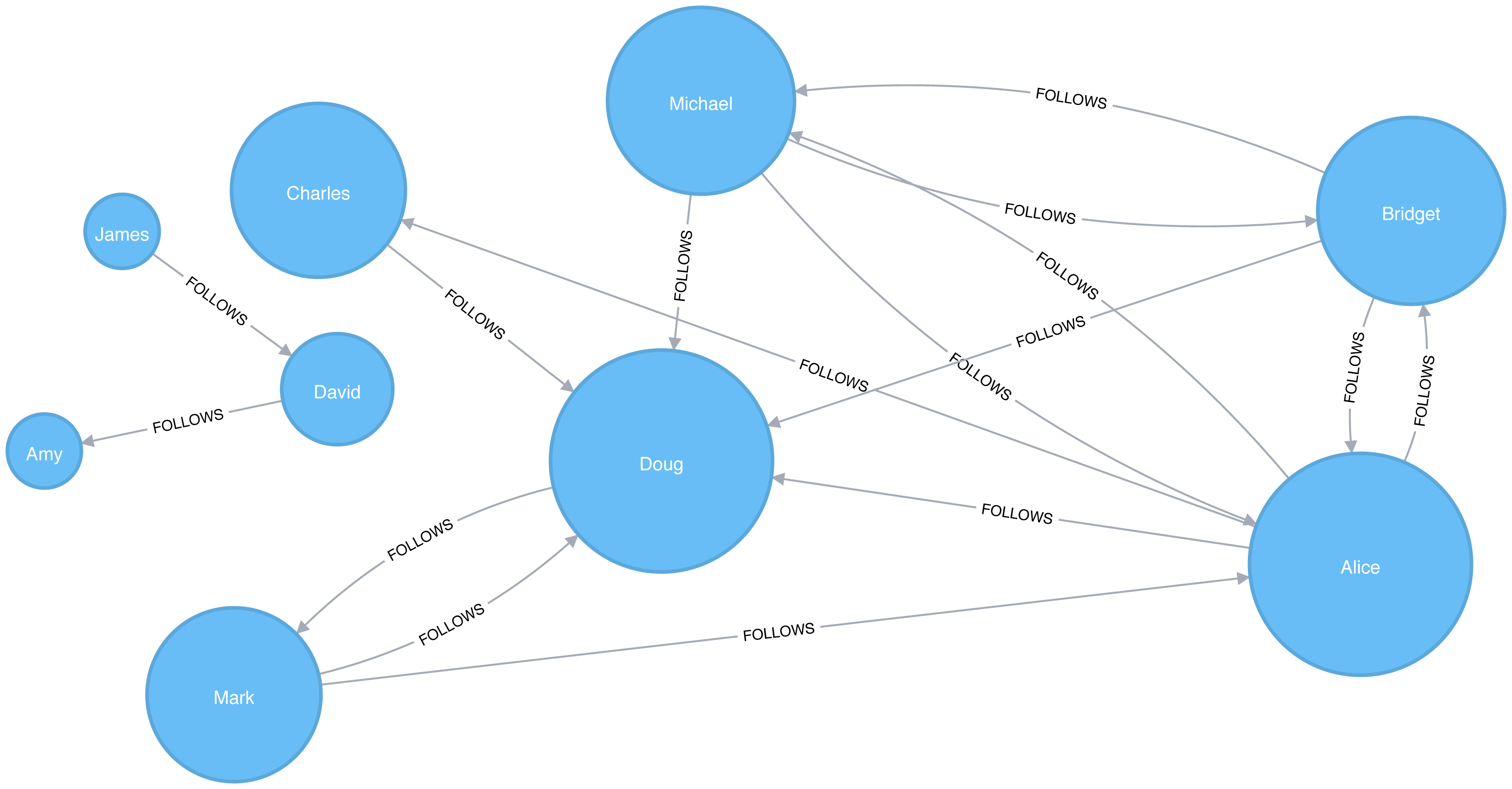
Figure 5-5. Visualization of Closeness Centrality
Now Figure 5-5 shows the results are more representative of the closeness of nodes to the entire graph. The scores for the members of the smaller subgraph (David, Amy, and James) have been dampened and now have the lowest scores of all users. This makes sense as they are the most isolated nodes. This formula is more useful for detecting the importance of a node across the entire graph rather than within their own subgraph.
In the next section we’ll learn about the Harmonic Centrality algorithm, which achieves similar results using another formula to calculate closeness.
Closeness Centrality Variation: Harmonic Centrality
Harmonic Centrality (also known as valued centrality) is a variant of Closeness Centrality, invented to solve the original problem with unconnected graphs. In “Harmony in a Small World” 8 Marchiori and Latora proposed this concept as a practical representation of an average shortest path.
When calculating the closeness score for each node, rather than summing the distances of a node to all other nodes, it sums the inverse of those distances. This means that infinite values become irrelevant.
The raw harmonic centrality for a node is calculated using the following formula:
where:
-
uis a node -
nis the number of nodes in the graph -
d(u,v)is the shortest-path distance between another nodevandu
As with closeness centrality we also calculate a normalized harmonic centrality with the following formula:
In this formula, ∞ values are handled cleanly.
Harmonic Centrality with Neo4j
The following query executes the Harmonic Centrality algorithm:
CALL algo.closeness.harmonic.stream("User","FOLLOWS")YIELD nodeId, centralityRETURNalgo.getNodeById(nodeId).idASuser, centralityORDER BYcentralityDESC
Running this procedure gives the following result:
| user | centrality |
|---|---|
Alice |
0.625 |
Doug |
0.625 |
Bridget |
0.5 |
Michael |
0.5 |
Charles |
0.4375 |
Mark |
0.4375 |
David |
0.25 |
Amy |
0.1875 |
James |
0.1875 |
The results from this algorithm differ from the original Closeness Centrality but are similar to those from the Wasserman and Faust improvement. Either algorithm can be used when working with graphs with more than one connected component.
Betweenness Centrality
Sometimes the most important cog in the system is not the one with the most overt power or the highest status. Sometimes it’s the middlemen that connect groups or the brokers with the most control over resources or the flow of information. Betweenness Centrality is a way of detecting the amount of influence a node has over the flow of information in a graph. It is typically used to find nodes that serve as a bridge from one part of a graph to another.
The Betweenness Centrality algorithm first calculates the shortest (weighted) path between every pair of nodes in a connected graph. Each node receives a score, based on the number of these shortest paths that pass through the node. The more shortest paths that a node lies on, the higher its score.
Betweenness Centrality was considered one of the “three distinct intuitive conceptions of centrality” when it was introduced by Linton Freeman in his 1971 paper A Set of Measures of Centrality Based on Betweenness. 9
Bridges and Control Points
A bridge in a network can be a node or a relationship. In a very simple graph, you can find them by looking for the node or relationship that if removed, would cause a section of the graph to become disconnected. However, as that’s not practical in a typical graph, we use a betweenness centrality algorithm. We can also measure the betweenness of a cluster by treating the group as a node.
A node is considered pivotal for two other nodes if it lies on every shortest path between those nodes as shown in Figure 5-6.
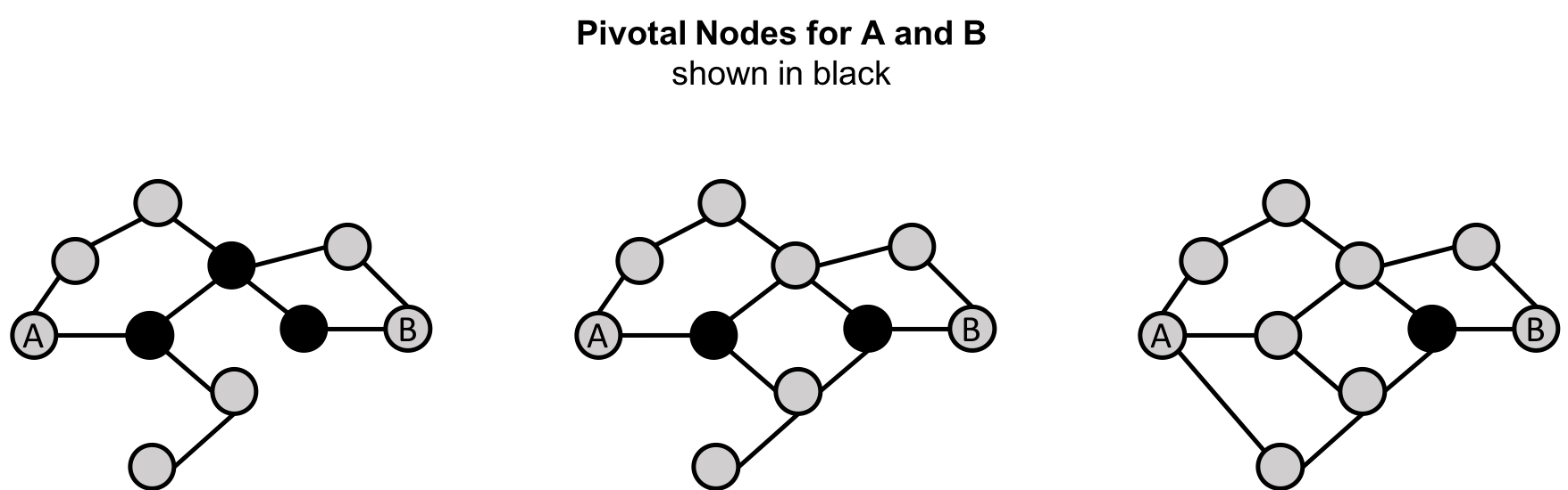
Figure 5-6. Pivotal nodes lie on the every shortest path between two nodes. Creating more shortest paths, can reduce the number of pivotal nodes for uses such as risk mitigation.
Pivotal nodes play an important role in connecting other nodes - if you remove a pivotal node, the new shortest path for the original node pairs will be longer or more costly. This can be a consideration for evaluating single points of vulnerability.
Calculating Betweenness Centrality
The Betweenness Centrality of a node is calculated by adding the results of the below formula for all shortest-paths:
where:
-
uis a node -
pis the total number of shortest-path between nodessandt -
p(u)is the number shortest-path between nodessandtthat pass through nodeu
Figure 5-7 describes the steps for working out Betweenness Centrality.
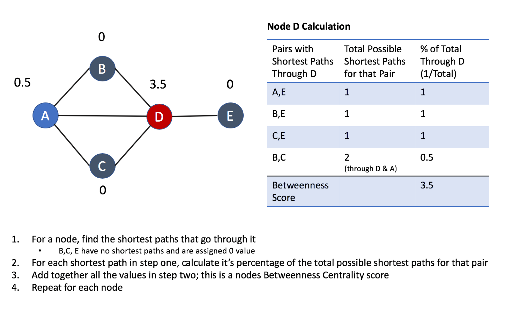
Figure 5-7. Basic Concepts for Calculating Betweenness Centrality
When Should I Use Betweenness Centrality?
Betweenness Centrality applies to a wide range of problems in real-world networks. We use it to find bottlenecks, control points, and vulnerabilities.
Example use cases include:
-
Betweenness Centrality is used to identify influencers in various organizations. Powerful individuals are not necessarily in management positions, but can be found in “brokerage positions” using Betweenness Centrality. Removal of such influencers seriously destabilize the organization. This might be a welcome disruption by law enforcement if the organization is criminal, or may be a disaster if a business loses key staff it never knew about. More details are found in Brokerage qualifications in ringing operations 10 by Carlo Morselli and Julie Roy.
-
Betweenness Centrality uncovers key transfer points in networks such electrical grids. Counterintuitively, removal of specific bridges can actually improve overall robustness by “islanding” disturbances. Research details are included in Robustness of the European power grids under intentional attack 11 by Sol´e R., Rosas-Casals M., Corominas-Murtral B., and Valverde S.
-
Betweenness Centrality is also used to help microbloggers spread their reach on Twitter, with a recommendation engine for targeting influencers. This approach is described in Making Recommendations in a Microblog to Improve the Impact of a Focal User. 12
Tip
Betweenness Centrality makes the assumption that all communication between nodes happens along the shortest path and with the same frequency, which isn’t always the case in real life. Therefore, it doesn’t give us a perfect view of the most influential nodes in a graph, but rather a good representation. Newman explains in more detail on page 186 of Networks: An Introduction. 13
Betweenness Centrality with Neo4j
Apache Spark doesn’t have a built in algorithm for Betweenness Centrality so we’ll demonstrate this algorithm using Neo4j. A call to the following procedure will calculate the Betweenness Centrality for each of the nodes in our graph:
CALL algo.betweenness.stream("User","FOLLOWS")YIELD nodeId, centralityRETURNalgo.getNodeById(nodeId).idASuser, centralityORDER BYcentralityDESC
Running this procedure gives the following result:
| user | centrality |
|---|---|
Alice |
10.0 |
Doug |
7.0 |
Mark |
7.0 |
David |
1.0 |
Bridget |
0.0 |
Charles |
0.0 |
Michael |
0.0 |
Amy |
0.0 |
James |
0.0 |
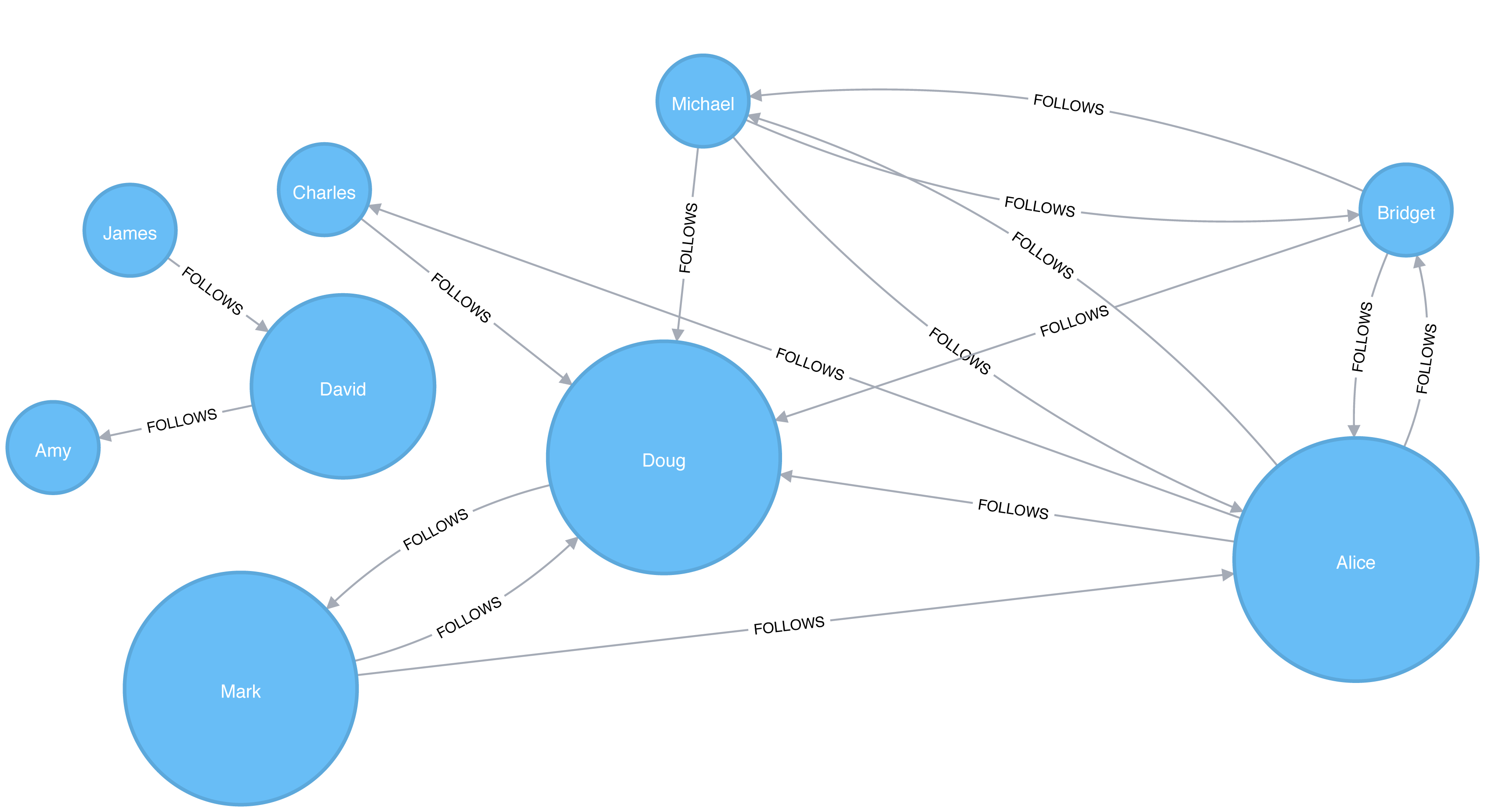
Figure 5-8. Visualization of Betweenness Centrality
As we can see in Figure 5-8, Alice is the main broker in this network, but Mark and Doug aren’t far behind. In the smaller sub graph all shortest paths go between David so he is important for information flow amongst those nodes.
Warning
For large graphs, exact centrality computation isn’t practical. The fastest known algorithm for exactly computing betweenness of all the nodes has a run time proportional to the product of the number of nodes and the number of relationships.
We may want to filter down to a subgraph first or use an approximation algorithm (shown later) that works with a subset of nodes.
We can now join our two disconnected components together by introducing a new user called Jason. Jason follows and is followed by people from both groups of users.
WITH["James","Michael","Alice","Doug","Amy"]ASexistingUsersMATCH(existing:User)WHEREexisting.idINexistingUsersMERGE (newUser:User {id:"Jason"})MERGE (newUser)<-[:FOLLOWS]-(existing)MERGE (newUser)-[:FOLLOWS]->(existing)
If we re-run the algorithm we’ll see this output:
| user | centrality |
|---|---|
Jason |
44.33333333333333 |
Doug |
18.333333333333332 |
Alice |
16.666666666666664 |
Amy |
8.0 |
James |
8.0 |
Michael |
4.0 |
Mark |
2.1666666666666665 |
David |
0.5 |
Bridget |
0.0 |
Charles |
0.0 |
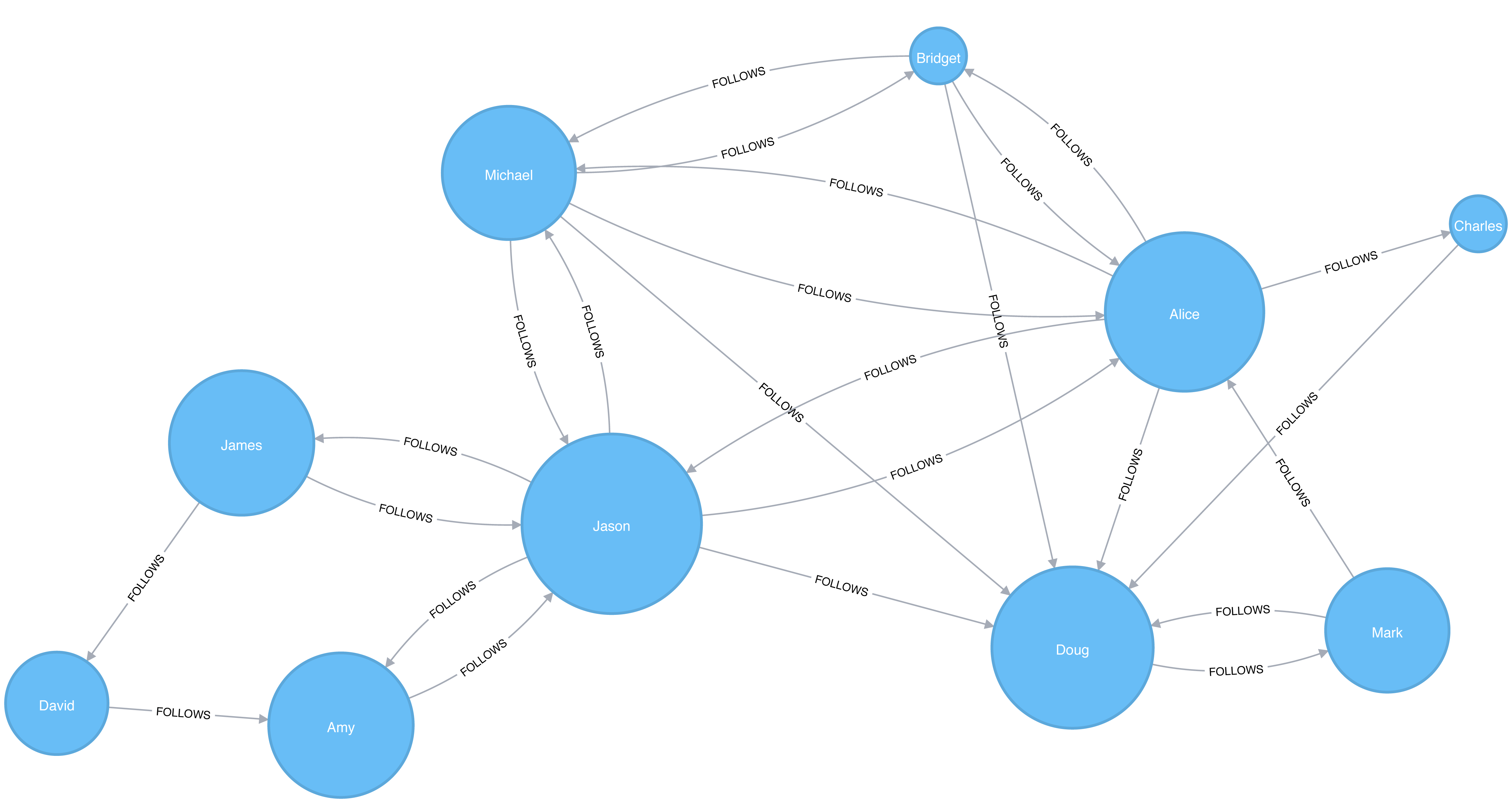
Figure 5-9. Visualization of Betweenness Centrality with Jason
Jason has the highest score because communication between the two sets of users will pass through him. Jason can be said to act as a local bridge between the two sets of users, which is illustrated in Figure 5-9.
Before we move onto the next section reset our graph by deleting Jason and his relationships:
MATCH(user:User {id:"Jason"})DETACHDELETEuser
Betweenness Centrality Variation: Randomized-Approximate Brandes
Recall that calculating the exact betweenness centrality on large graphs can be very expensive. We could therefore choose to use an approximation algorithm that runs much quicker and still provides useful (albeit imprecise) information.
The Randomized-Approximate Brandes, or in short RA-Brandes, algorithm is the best-known algorithm for calculating an approximate score for betweenness centrality. Rather than calculating the shortest path between every pair of nodes, the RA-Brandes algorithm considers only a subset of nodes. Two common strategies for selecting the subset of nodes are:
Random
Nodes are selected uniformly, at random, with defined probability of selection. The default probability is . If the probability is 1, the algorithm works the same way as the normal Betweenness Centrality algorithm, where all nodes are loaded.
Degree
Nodes are selected randomly, but those whose degree is lower than the mean are automatically excluded. (i.e. only nodes with a lot of relationships have a chance of being visited).
As a further optimization, you could limit the depth used by the Shortest Path algorithm, which will then provide a subset of all shortest paths.
Approximation of Betweenness Centrality with Neo4j
The following query executes the RA-Brandes algorithm using the random selection method.
CALL algo.betweenness.sampled.stream("User","FOLLOWS", {strategy:"degree"})YIELD nodeId, centralityRETURNalgo.getNodeById(nodeId).idASuser, centralityORDER BYcentralityDESC
Running this procedure gives the following result:
| user | centrality |
|---|---|
Alice |
9.0 |
Mark |
9.0 |
Doug |
4.5 |
David |
2.25 |
Bridget |
0.0 |
Charles |
0.0 |
Michael |
0.0 |
Amy |
0.0 |
James |
0.0 |
Our top influencers are similar to before although Mark now has a higher ranking than Doug.
Due to the random nature of this algorithm we will see different results each time that we run it. On larger graphs this randomness will have less of an impact than it does on our small sample graph.
PageRank
PageRank is the best known of the Centrality algorithms and measures the transitive (or directional) influence of nodes. All the other Centrality algorithms we discuss measure the direct influence of a node, whereas PageRank considers the influence of your neighbors and their neighbors. For example, having a few powerful friends can make you more influential than just having a lot of less powerful friends. PageRank is computed by either iteratively distributing one node’s rank over its neighbors or by randomly traversing the graph and counting the frequency of hitting each node during these walks.
PageRank is named after Google co-founder Larry Page, who created it to rank websites in Google’s search results. The basic assumption is that a page with more incoming and influential incoming links is a more likely a credible source. PageRank counts the number, and quality, of incoming relationships to a node, which determines an estimation of how important that node is. Nodes with more sway over a network are presumed to have more incoming relationships from other influential nodes.
Influence
The intuition behind influence is that relationships to more important nodes contribute more to the influence of the node in question than equivalent connections to less important nodes. Measuring influence usually involves scoring nodes, often with weighted relationships, and then updating scores over many iterations. Sometimes all nodes are scored and sometimes a random selection is used as a representative distribution.
Keep in mind that centrality measures the importance of a node in comparison to other nodes. It is a ranking among the potential impact of nodes, not a measure of actual impact. For example, you might identify the 2 people with the highest centrality in a network but perhaps set policies or cultural norms actually have more effect. Quantifying actual impact is an active research area to develop more node influence metrics.
The PageRank Formula
PageRank is defined in the original Google paper as follows:
where:
-
we assume that a page u has citations from pages T1 to Tn
-
dis a damping factor which is set between 0 and 1. It is usually set to 0.85. You can think of this as the probability that a user will continue clicking. This helps minimize Rank Sink, explained below. -
1-dis the probability that a node is reached directly without following any relationships -
C(T)is defined as out-degree of a node T.
Figure 5-10 walks through a small example of how PageRank would continue to update the rank of a node until it converges or meets the set number of iterations.
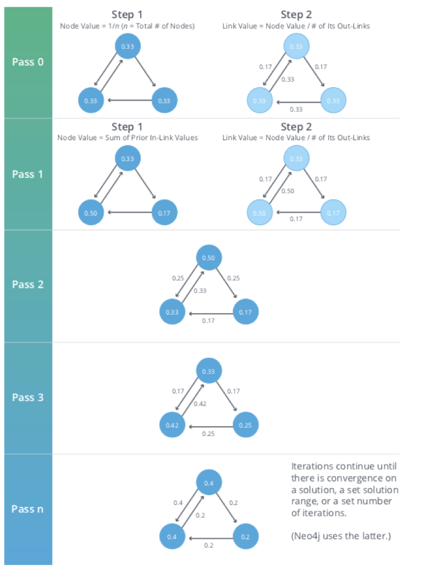
Figure 5-10. Each iteration of PageRank has two calculation steps: one to update node values and one to update link values.
Iteration, Random Surfers and Rank Sinks
PageRank is an iterative algorithm that runs either until scores converge or a simply for a set number of iterations.
Conceptually, PageRank assumes there is a web surfer visiting pages by following links or by using a random URL.
A damping factor d defines the probability that the next click will be through a link.
You can think of it as the probability that a surfer will become bored and randomly switches to a page.
A PageRank score represents the likelihood that a page is visited through an incoming link and not randomly.
A node, or group of nodes, without outgoing relationships (also called dangling nodes), can monopolize the PageRank score. This is a rank sink. You can imagine this as a surfer that gets stuck on a page, or a subset of pages, with no way out. Another difficulty is created by nodes that point only to each other in a group. Circular references cause the increase in their ranks as the surfer bounces back and forth among nodes. These situations are protrayed in Figure 5-11.
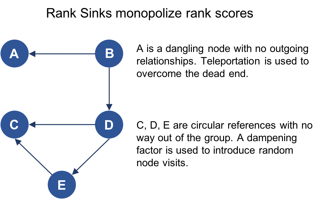
Figure 5-11. Rank Sink
There are two strategies used to avoid rank sink.
First, when a node is reached with no outgoing relationships, PageRank assumes outgoing relationships to all nodes.
Traversing these invisible links is sometimes called teleportation.
Second, the dampening factor provides another opportunity to avoid sinks by introducing a probability for direct link versus random node visitation.
When you set d to 0.85, a completely random node is visited 15% of the time.
Although the original formula recommends a dampening factor of 0.85, its initial use was on the World Wide Web with a power law distribution of links where most pages have very few links and a few pages have many. Lowering our damping factor decreases the likelihood of following long relationship paths before taking a random jump. In turn this increases the contribution of immediate neighbors to a node’s score and rank.
If you see unexpected results from running the algorithm, it is worth doing some exploratory analysis of the graph to see if any of these problems are the cause. You can read “The Google PageRank Algorithm and How It Works”14 to learn more.
When should I use PageRank?
PageRank is now used in many domains outside Web indexing. Use this algorithm anytime you’re looking for broad influence over a network. For instance, if you’re looking to target a gene that has the highest overall impact to a biological function, it may not be the most connected one. It may, in fact, be the gene with relationships with other, more significant functions.
Example use cases include:
-
Twitter uses Personalized PageRank to present users with recommendations of other accounts that they may wish to follow. The algorithm is run over a graph that contains shared interests and common connections. Their approach is described in more detail in WTF: The Who to Follow Service at Twitter. 15
-
PageRank has been used to rank public spaces or streets, predicting traffic flow and human movement in these areas. The algorithm is run over a graph of road intersections, where the PageRank score reflects the tendency of people to park, or end their journey, on each street. This is described in more detail in Self-organized Natural Roads for Predicting Traffic Flow: A Sensitivity Study. 16
-
PageRank is also used as part of an anomaly and fraud detection system in the healthcare and insurance industries. It helps reveal doctors or providers that are behaving in an unusual manner and then feeds the score into a machine learning algorithm.
David Gleich describes many more uses for the algorithm in his paper, PageRank Beyond the Web. 17
PageRank with Apache Spark
Now we’re ready to execute the PageRank algorithm.
GraphFrames supports two implementations of PageRank:
-
The first implementation runs PageRank for a fixed number of iterations. This can be run by setting the
maxIterparameter. -
The second implementation runs PageRank until convergence. This can be run by setting the
tolparameter.
PageRank with fixed number of iterations
Let’s see an example of the fixed iterations approach:
results=g.pageRank(resetProbability=0.15,maxIter=20)results.vertices.sort("pagerank",ascending=False).show()
Tip
Notice in Apache Spark, that the dampening factor is more intuitively called the reset probability with the inverse value.
In other words, resetProbability=0.15 in this example is equivalent to dampingFactor:0.85 in Neo4j.
If we run that code in pyspark we’ll see this output:
| id | pagerank |
|---|---|
Doug |
2.2865372087512252 |
Mark |
2.1424484186137263 |
Alice |
1.520330830262095 |
Michael |
0.7274429252585624 |
Bridget |
0.7274429252585624 |
Charles |
0.5213852310709753 |
Amy |
0.5097143486157744 |
David |
0.36655842368870073 |
James |
0.1981396884803788 |
As we might expect, Doug has the highest PageRank because he is followed by all other users in his sub graph. Although Mark only has one follower, that follower is Doug, so Mark is also considered important in this graph. It’s not only the number of followers that is important, but also the importance of those followers.
PageRank until convergence
And now let’s try the convergence implementation which will run PageRank until it closes in on a solution within the set tolerance:
results=g.pageRank(resetProbability=0.15,tol=0.01)results.vertices.sort("pagerank",ascending=False).show()
If we run that code in pyspark we’ll see this output:
| id | pagerank |
|---|---|
Doug |
2.2233188859989745 |
Mark |
2.090451188336932 |
Alice |
1.5056291439101062 |
Michael |
0.733738785109624 |
Bridget |
0.733738785109624 |
Amy |
0.559446807245026 |
Charles |
0.5338811076334145 |
David |
0.40232326274180685 |
James |
0.21747203391449021 |
Tip
Although convergence on a perfect solution may sound ideal, in some scenarios PageRank cannot mathematically converge. For larger graphs, PageRank execution may be prohibitively long. A tolerance limit helps set an acceptable range for a converged result, but many choose to use or combine with the maximum iteration option instead. The maximum iteration setting will generally provide more performance consistency. Regardless of which option you choose, you may need to test several different limits to find what works for your dataset. Larger graphs typcially require more iterations or smaller tolerance than medium sized graphs for better accuracy.
PageRank with Neo4j
We also can run PageRank in Neo4j. A call to the following procedure will calculate the PageRank for each of the nodes in our graph:
CALL algo.pageRank.stream('User','FOLLOWS', {iterations:20, dampingFactor:0.85})YIELD nodeId, scoreRETURNalgo.getNodeById(nodeId).idASpage, scoreORDER BYscoreDESC
Running this procedure gives the following result:
| page | score |
|---|---|
Doug |
1.6704119999999998 |
Mark |
1.5610085 |
Alice |
1.1106700000000003 |
Bridget |
0.535373 |
Michael |
0.535373 |
Amy |
0.385875 |
Charles |
0.3844895 |
David |
0.2775 |
James |
0.15000000000000002 |
As with the Apache Spark example, Doug is the most influential user and Mark follows closely after as the only user that Doug follows. We can see the importance of nodes relative to each other in Figure 5-12.
Note
PageRank implementations vary.
This can produce different scoring even when ordering is the same.
Neo4j initializes nodes using a value of 1-the dampening factor whereas Spark uses a value of 1.
In this case, the relative rankings (the goal of PageRank) are identical but the underlying score values used to reach those results are different.
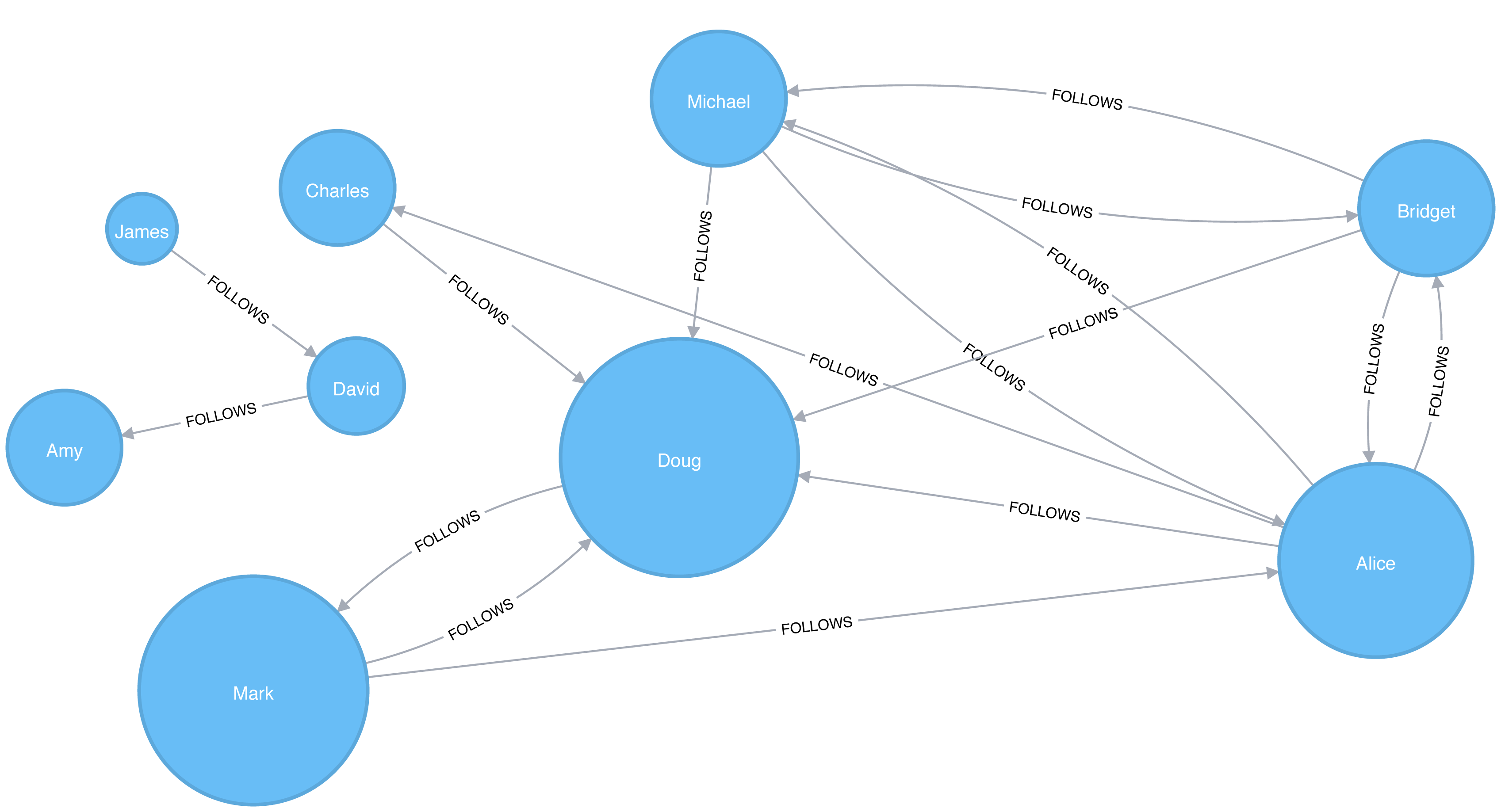
Figure 5-12. Visualization of PageRank
PageRank Variation: Personalized PageRank
Personalized PageRank (PPR) is a variant of the PageRank algorithm which calculates the importance of nodes in a graph from the perspective of a specific node. For PPR, random jumps refer back to a given set of starting nodes. This biases results towards, or personalizes for, the start node. This bias and localization make it useful for hihgly targeted recommendations.
Personalized PageRank with Apache Spark
We can calculate the Personalized PageRank for a given node by passing in the sourceId parameter.
The following code calculates the Personalized PageRank for Doug:
me="Doug"results=g.pageRank(resetProbability=0.15,maxIter=20,sourceId=me)people_to_follow=results.vertices.sort("pagerank",ascending=False)already_follows=list(g.edges.filter(f"src = '{me}'").toPandas()["dst"])people_to_exclude=already_follows+[me]people_to_follow[~people_to_follow.id.isin(people_to_exclude)].show()
The results of this query could be used to make recommendations for people that Doug should follow. Notice that we’re also making sure that we exclude people that Doug already follows as well as himself from our final result.
If we run that code in pyspark we’ll see this output:
| id | pagerank |
|---|---|
Alice |
0.1650183746272782 |
Michael |
0.048842467744891996 |
Bridget |
0.048842467744891996 |
Charles |
0.03497796119878669 |
David |
0.0 |
James |
0.0 |
Amy |
0.0 |
Alice is the best suggestion for somebody that Doug should follow, but we might suggest Michael and Bridget as well.
Summary
Centrality algorithms are an excellent tool for identifying influencers in a network. In this chapter we’ve learned about the prototypical Centrality algorithms: Degree Centrality, Closeness Centrality, Betweenness Centrality, and PageRank. We’ve also covered several variations to deal with issues such as long run times and isolated components, as well as options for alternative uses.
There are many, wide-ranging uses for Centrality algorithms and we encourage you to put them to work in your analyses. Apply what you’ve learned to locate optimal touch points for disseminating information, find the hidden brokers that control the flow of resources, and uncover the indirect power players lurking in the shadows.
Next, we’ll turn to turn Community Detection algorithms that look at groups and partitions.
1 http://leonidzhukov.net/hse/2014/socialnetworks/papers/freeman79-centrality.pdf
2 https://www.brandwatch.com/blog/react-influential-men-and-women-2017/
3 https://link.springer.com/chapter/10.1007/978-3-319-23461-8_11
4 http://www.orgnet.com/MappingTerroristNetworks.pdf
5 http://www.analytictech.com/borgatti/papers/centflow.pdf
6 https://www.aclweb.org/anthology/I/I13/I13-1102.pdf
7 pg. 201 of Wasserman, S. and Faust, K., Social Network Analysis: Methods and Applications, 1994, Cambridge University Press.
8 https://arxiv.org/pdf/cond-mat/0008357.pdf
9 http://moreno.ss.uci.edu/23.pdf
10 http://archives.cerium.ca/IMG/pdf/Morselli_and_Roy_2008_.pdf
11 More https://arxiv.org/pdf/0711.3710.pdf
12 ftp://ftp.umiacs.umd.edu/incoming/louiqa/PUB2012/RecMB.pdf
13 https://global.oup.com/academic/product/networks-9780199206650?cc=us&lang=en&
14 http://www.cs.princeton.edu/~chazelle/courses/BIB/pagerank.htm
15 https://web.stanford.edu/~rezab/papers/wtf_overview.pdf
Figure 5-1. Graph model