Summarizing Data

In Chapter 8, you looked at breaking up text content into n-grams, or sets of phrases that are n words in length. At a basic level, this can be used to determine which sets of words and phrases tend to be most commonly used in a section of text. In addition, it can be used to create natural-sounding data summaries by going back to the original text and extracting sentences around some of these most popular phrases.

One piece of sample text you’ll be using to do this is the inauguration speech of the ninth president of the United States, William Henry Harrison. Harrison’s presidency sets two records in the history of the office: one for the longest inauguration speech, and another for the shortest time in office, 32 days.

You’ll use the full text of this speech as the source for many of the code samples in this chapter.

Slightly modifying the n-gram used to find code in Chapter 8, you can produce code that looks for sets of 2-grams and returns a Counter object with all 2-grams:

from urllib.request import urlopen
from bs4 import BeautifulSoup
import re
import string
from collections import Counter

def cleanSentence(sentence):
    sentence = sentence.split(' ')
    sentence = [word.strip(string.punctuation+string.whitespace)
        for word in sentence]
    sentence = [word for word in sentence if len(word) > 1
        or (word.lower() == 'a' or word.lower() == 'i')]
    return sentence

def cleanInput(content):
    content = content.upper()
    content = re.sub('\n', ' ', content)
    content = bytes(content, "UTF-8")
    content = content.decode("ascii", "ignore")
    sentences = content.split('. ')
    return [cleanSentence(sentence) for sentence in sentences]

def getNgramsFromSentence(content, n):
    output = []
    for i in range(len(content)-n+1):
        output.append(content[i:i+n])
    return output

def getNgrams(content, n):
    content = cleanInput(content)
    ngrams = Counter()
    ngrams_list = []
    for sentence in content:
        newNgrams = [' '.join(ngram) for ngram in
            getNgramsFromSentence(sentence, 2)]
        ngrams_list.extend(newNgrams)
        ngrams.update(newNgrams)
    return(ngrams)


content = str(
      urlopen('http://pythonscraping.com/files/inaugurationSpeech.txt')
        .read(), 'utf-8')
ngrams = getNgrams(content, 2)
print(ngrams)

The output produces, in part:

Counter({'OF THE': 213, 'IN THE': 65, 'TO THE': 61, 'BY THE': 41,
'THE CONSTITUTION': 34, 'OF OUR': 29, 'TO BE': 26, 'THE PEOPLE': 24,
'FROM THE': 24, 'THAT THE': 23,...

Of these 2-grams, “the constitution” seems like a reasonably popular subject in the speech, but “of the,” “in the,” and “to the” don’t seem especially noteworthy. How can you automatically get rid of unwanted words in an accurate way?

Fortunately, there are people out there who carefully study the differences between “interesting” words and “uninteresting” words, and their work can help us do just that. Mark Davies, a linguistics professor at Brigham Young University, maintains the Corpus of Contemporary American English, a collection of over 450 million words from the last decade or so of popular American publications.

The list of 5,000 most frequently found words is available for free, and fortunately, this is far more than enough to act as a basic filter to weed out the most common 2-grams. Just the first 100 words vastly improves the results, with the addition of an isCommon function:

def isCommon(ngram):
    commonWords = ['THE', 'BE', 'AND', 'OF', 'A', 'IN', 'TO', 'HAVE', 'IT', 'I',
        'THAT', 'FOR', 'YOU', 'HE', 'WITH', 'ON', 'DO', 'SAY', 'THIS', 'THEY',
        'IS', 'AN', 'AT', 'BUT', 'WE', 'HIS', 'FROM', 'THAT', 'NOT', 'BY',
        'SHE', 'OR', 'AS', 'WHAT', 'GO', 'THEIR', 'CAN', 'WHO', 'GET', 'IF',
        'WOULD', 'HER', 'ALL', 'MY', 'MAKE', 'ABOUT', 'KNOW', 'WILL', 'AS',
        'UP', 'ONE', 'TIME', 'HAS', 'BEEN', 'THERE', 'YEAR', 'SO', 'THINK',
        'WHEN', 'WHICH', 'THEM', 'SOME', 'ME', 'PEOPLE', 'TAKE', 'OUT', 'INTO',
        'JUST', 'SEE', 'HIM', 'YOUR', 'COME', 'COULD', 'NOW', 'THAN', 'LIKE',
        'OTHER', 'HOW', 'THEN', 'ITS', 'OUR', 'TWO', 'MORE', 'THESE', 'WANT',
        'WAY', 'LOOK', 'FIRST', 'ALSO', 'NEW', 'BECAUSE', 'DAY', 'MORE', 'USE',
        'NO', 'MAN', 'FIND', 'HERE', 'THING', 'GIVE', 'MANY', 'WELL']
    for word in ngram:
        if word in commonWords:
            return True
    return False

This produces the following 2-grams that were found more than twice in the text body:

Counter({'UNITED STATES': 10, 'EXECUTIVE DEPARTMENT': 4, 
'GENERAL GOVERNMENT': 4, 'CALLED UPON': 3, 'CHIEF MAGISTRATE': 3,
'LEGISLATIVE BODY': 3, 'SAME CAUSES': 3, 'GOVERNMENT SHOULD': 3,
'WHOLE COUNTRY': 3,...

Appropriately enough, the first two items in the list are “United States” and “executive department,” which you would expect for a presidential inauguration speech.

It’s important to note that you are using a list of common words from relatively modern times to filter the results, which might not be appropriate given that the text was written in 1841. However, because you’re using only the first 100 or so words on the list—which you can assume are more stable over time than, say, the last 100 words—and you appear to be getting satisfactory results, you can likely save yourself the effort of tracking down or creating a list of the most common words from 1841 (although such an effort might be interesting).

Now that some key topics have been extracted from the text, how does this help you write text summaries? One way is to search for the first sentence that contains each “popular” n-gram, the theory being that the first instance will yield a satisfactory overview of the body of the content. The first five most popular 2-grams yield these bullet points:

• The Constitution of the United States is the instrument containing this grant of power to the several departments composing the Government.

• Such a one was afforded by the executive department constituted by the Constitution.

• The General Government has seized upon none of the reserved rights of the States.

• Called from a retirement which I had supposed was to continue for the residue of my life to fill the chief executive office of this great and free nation, I appear before you, fellow-citizens, to take the oaths which the constitution prescribes as a necessary qualification for the performance of its duties; and in obedience to a custom coeval with our government and what I believe to be your expectations I proceed to present to you a summary of the principles which will govern me in the discharge of the duties which I shall be called upon to perform.

• The presses in the necessary employment of the Government should never be used to “clear the guilty or to varnish crime.”

Sure, it might not be published in CliffsNotes any time soon, but considering that the original document was 217 sentences in length, and the fourth sentence (“Called from a retirement...”) condenses the main subject down fairly well, it’s not too bad for a first pass.

With longer blocks of text, or more varied text, it may be worth looking at 3-grams or even 4-grams when retrieving the “most important” sentences of a passage. In this case, only one 3-gram is used multiple times and that is “exclusive metallic currency”—hardly a defining phrase for a presidential inauguration speech. With longer passages, using 3-grams may be appropriate.

Another approach is to look for sentences that contain the most popular n-grams. These will, of course, tend to be longer sentences, so if that becomes a problem, you can look for sentences with the highest percentage of words that are popular n-grams, or create a scoring metric of your own, combining several techniques.

Markov Models

You might have heard of Markov text generators. They’ve become popular for entertainment purposes, as in the “That can be my next tweet!” app, as well as their use for generating real-sounding spam emails to fool detection systems.

All of these text generators are based on the Markov model, which is often used to analyze large sets of random events, where one discrete event is followed by another discrete event with a certain probability.

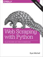
For example, you might build a Markov model of a weather system, as illustrated in Figure 9-1.

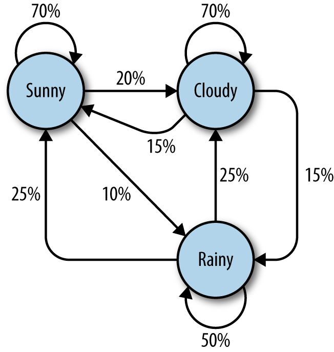
Figure 9-1. Markov model describing a theoretical weather system

In this model, each sunny day has a 70% chance of the following day also being sunny, with a 20% chance of the following day being cloudy with a mere 10% chance of rain. If the day is rainy, there is a 50% chance of rain the following day, a 25% chance of sun, and a 25% chance of clouds.

You might note several properties in this Markov model:

• All percentages leading away from any one node must add up to exactly 100%. No matter how complicated the system, there must always be a 100% chance that it can lead somewhere else in the next step.

• Although there are only three possibilities for the weather at any given time, you can use this model to generate an infinite list of weather states.

• Only the state of the current node you are on influences where you will go to next. If you’re on the Sunny node, it doesn’t matter if the preceding 100 days were sunny or rainy—the chances of sun the next day are exactly the same: 70%.

• It might be more difficult to reach some nodes than others. The math behind this is reasonably complicated, but it should be fairly easy to see that Rainy (with less than “100%” worth of arrows pointing toward it) is a much less likely state to reach in this system, at any given point in time, than Sunny or Cloudy.

Obviously, this is a simple system, and Markov models can grow arbitrarily large. Google’s page-rank algorithm is based partly on a Markov model, with websites represented as nodes and inbound/outbound links represented as connections between nodes. The “likelihood” of landing on a particular node represents the relative popularity of the site. That is, if our weather system represented an extremely small internet, “rainy” would have a low page rank, while “cloudy” would have a high page rank.

With all of this in mind, let’s bring it back down to a more concrete example: analyzing and writing text.

Again using the inauguration speech of William Henry Harrison analyzed in the previous example, you can write the following code that generates arbitrarily long Markov chains (with the chain length set to 100) based on the structure of its text:

from urllib.request import urlopen
from random import randint

def wordListSum(wordList):
    sum = 0
    for word, value in wordList.items():
        sum += value
    return sum

def retrieveRandomWord(wordList):
    randIndex = randint(1, wordListSum(wordList))
    for word, value in wordList.items():
        randIndex -= value
        if randIndex <= 0:
            return word

def buildWordDict(text):
    # Remove newlines and quotes
    text = text.replace('\n', ' ');
    text = text.replace('"', '');

    # Make sure punctuation marks are treated as their own "words,"
    # so that they will be included in the Markov chain
    punctuation = [',','.',';',':']
    for symbol in punctuation:
        text = text.replace(symbol, ' {} '.format(symbol));

    words = text.split(' ')
    # Filter out empty words
    words = [word for word in words if word != '']

    wordDict = {}
    for i in range(1, len(words)):
        if words[i-1] not in wordDict:
                # Create a new dictionary for this word
            wordDict[words[i-1]] = {}
        if words[i] not in wordDict[words[i-1]]:
            wordDict[words[i-1]][words[i]] = 0
        wordDict[words[i-1]][words[i]] += 1
    return wordDict

text = str(urlopen('http://pythonscraping.com/files/inaugurationSpeech.txt')
          .read(), 'utf-8')
wordDict = buildWordDict(text)

#Generate a Markov chain of length 100
length = 100
chain = ['I']
for i in range(0, length):
    newWord = retrieveRandomWord(wordDict[chain[-1]])
    chain.append(newWord)

print(' '.join(chain))

The output of this code changes every time it is run, but here’s an example of the uncannily nonsensical text it will generate:

I sincerely believe in Chief Magistrate to make all necessary sacrifices and
oppression of the remedies which we may have occurred to me in the arrangement 
and disbursement of the democratic claims them , consolatory to have been best 
political power in fervently commending every other addition of legislation , by
the interests which violate that the Government would compare our aboriginal 
neighbors the people to its accomplishment . The latter also susceptible of the 
Constitution not much mischief , disputes have left to betray . The maxim which 
may sometimes be an impartial and to prevent the adoption or 

So what’s going on in the code?

The function buildWordDict takes in the string of text, which was retrieved from the internet. It then does some cleaning and formatting, removing quotes and putting spaces around other punctuation so it is effectively treated as a separate word. After this, it builds a two-dimensional dictionary—a dictionary of dictionaries—that has the following form:

{word_a : {word_b : 2, word_c : 1, word_d : 1},
 word_e : {word_b : 5, word_d : 2},...}

In this example dictionary, “word_a” was found four times, two instances of which were followed by “word_b,” one instance followed by “word_c,” and one instance followed by “word_d.” “Word_e” was followed seven times, five times by “word_b” and twice by “word_d.”

If we were to draw a node model of this result, the node representing word_a would have a 50% arrow pointing toward “word_b” (which followed it two out of four times), a 25% arrow pointing toward “word_c,” and a 25% arrow pointing toward “word_d.”

After this dictionary is built up, it can be used as a lookup table to see where to go next, no matter which word in the text you happen to be on.³ Using the sample dictionary of dictionaries, you might currently be on “word_e,” which means that you’ll pass the dictionary {word_b : 5, word_d: 2} to the retrieveRandomWord function. This function in turn retrieves a random word from the dictionary, weighted by the number of times it occurs.

By starting with a random starting word (in this case, the ubiquitous “I”), you can traverse through the Markov chain easily, generating as many words as you like.

These Markov chains tend to improve in their “realism” as more text is collected, especially from sources with similar writing styles. Although this example used 2-grams to create the chain (where the previous word predicts the next word) 3-grams or higher-order n-grams can be used, where two or more words predict the next word.

Although entertaining, and a great use for megabytes of text that you might have accumulated during web scraping, applications like these can make it difficult to see the practical side of Markov chains. As mentioned earlier in this section, Markov chains model how websites link from one page to the next. Large collections of these links as pointers can form weblike graphs that are useful to store, track, and analyze. In this way, Markov chains form the foundation for both how to think about web crawling, and how your web crawlers can think.

import pymysql

conn = pymysql.connect(host='127.0.0.1', unix_socket='/tmp/mysql.sock',
    user='', passwd='', db='mysql', charset='utf8')
cur = conn.cursor()
cur.execute('USE wikipedia')

def getUrl(pageId):
    cur.execute('SELECT url FROM pages WHERE id = %s', (int(pageId)))
    return cur.fetchone()[0]

def getLinks(fromPageId):
    cur.execute('SELECT toPageId FROM links WHERE fromPageId = %s',
        (int(fromPageId)))
    if cur.rowcount == 0:
        return []
    return [x[0] for x in cur.fetchall()]

def searchBreadth(targetPageId, paths=[[1]]):
    newPaths = []
    for path in paths:
        links = getLinks(path[-1])
        for link in links:
            if link == targetPageId:
                return path + [link]
            else:
                newPaths.append(path+[link])
    return searchBreadth(targetPageId, newPaths)
                
nodes = getLinks(1)
targetPageId = 28624
pageIds = searchBreadth(targetPageId)
for pageId in pageIds:
    print(getUrl(pageId))

/wiki/Kevin_Bacon
/wiki/Primetime_Emmy_Award_for_Outstanding_Lead_Actor_in_a_
Miniseries_or_a_Movie
/wiki/Gary_Gilmore
/wiki/Eric_Idle

Natural Language Toolkit

So far, this chapter has focused primarily on the statistical analysis of words in bodies of text. Which words are most popular? Which words are unusual? Which words are likely to come after which other words? How are they grouped together? What you are missing is understanding, to the extent that you can, what the words represent.

The Natural Language Toolkit (NLTK) is a suite of Python libraries designed to identify and tag parts of speech found in natural English text. Its development began in 2000, and over the past 15 years, dozens of developers around the world have contributed to the project. Although the functionality it provides is tremendous (entire books are devoted to NLTK), this section focuses on just a few of its uses.

Installation and Setup

The nltk module can be installed in the same way as other Python modules, either by downloading the package through the NLTK website directly or by using any number of third-party installers with the keyword “nltk.” For complete installation instructions, see the NLTK website.

After installing the module, it’s a good idea to download its preset text repositories so you can try the features more easily. Type this on the Python command line:

>>> import nltk
>>> nltk.download()

This opens the NLTK Downloader (Figure 9-2).

I recommend installing all of the available packages when first trying out the NLTK corpus. You can easily uninstall packages at any time.

Figure 9-2. The NLTK Downloader lets you browse and download optional packages and text libraries associated with the nltk module

from nltk import word_tokenize
from nltk import Text

tokens = word_tokenize('Here is some not very interesting text')
text = Text(tokens)

from nltk.book import *

*** Introductory Examples for the NLTK Book ***
Loading text1, ..., text9 and sent1, ..., sent9
Type the name of the text or sentence to view it.
Type: 'texts()' or 'sents()' to list the materials.
text1: Moby Dick by Herman Melville 1851
text2: Sense and Sensibility by Jane Austen 1811
text3: The Book of Genesis
text4: Inaugural Address Corpus
text5: Chat Corpus
text6: Monty Python and the Holy Grail
text7: Wall Street Journal
text8: Personals Corpus
text9: The Man Who Was Thursday by G . K . Chesterton 1908

>>> len(text6)/len(set(text6))
7.833333333333333

>>> from nltk import FreqDist
>>> fdist = FreqDist(text6)
>>> fdist.most_common(10)
[(':', 1197), ('.', 816), ('!', 801), (',', 731), ("'", 421), ('[', 3
19), (']', 312), ('the', 299), ('I', 255), ('ARTHUR', 225)]
>>> fdist["Grail"]
34

>>> from nltk import bigrams
>>> bigrams = bigrams(text6)
>>> bigramsDist = FreqDist(bigrams)
>>> bigramsDist[('Sir', 'Robin')]
18

>>> from nltk import ngrams
>>> fourgrams = ngrams(text6, 4)
>>> fourgramsDist = FreqDist(fourgrams)
>>> fourgramsDist[('father', 'smelt', 'of', 'elderberries')]
1

from nltk.book import *
from nltk import ngrams
fourgrams = ngrams(text6, 4)
for fourgram in fourgrams: 
    if fourgram[0] == 'coconut': 
        print(fourgram)

>>> from nltk.book import *
>>> from nltk import word_tokenize
>>> text = word_tokenize('Strange women lying in ponds distributing swords'\
'is no basis for a system of government.')
>>> from nltk import pos_tag
>>> pos_tag(text)
[('Strange', 'NNP'), ('women', 'NNS'), ('lying', 'VBG'), ('in', 'IN')
, ('ponds', 'NNS'), ('distributing', 'VBG'), ('swords', 'NNS'), ('is'
, 'VBZ'), ('no', 'DT'), ('basis', 'NN'), ('for', 'IN'), ('a', 'DT'), 
('system', 'NN'), ('of', 'IN'), ('government', 'NN'), ('.', '.')]

>>> text = word_tokenize('The dust was thick so he had to dust')
>>> pos_tag(text)
[('The', 'DT'), ('dust', 'NN'), ('was', 'VBD'), ('thick', 'JJ'), ('so', 'RB'), ('he', 'PRP'), ('had', 'VBD'), ('to', 'TO'), ('dust', 'VB')]

from nltk import word_tokenize, sent_tokenize, pos_tag
sentences = sent_tokenize('Google is one of the best companies in the world.'\
' I constantly google myself to see what I\'m up to.')
nouns = ['NN', 'NNS', 'NNP', 'NNPS']

for sentence in sentences: 
    if 'google' in sentence.lower(): 
        taggedWords = pos_tag(word_tokenize(sentence)) 
            for word in taggedWords: 
                if word[0].lower() == 'google' and word[1] in nouns: 
                    print(sentence)

Additional Resources

Processing, analyzing, and understanding natural language by machine is one of the most difficult tasks in computer science, and countless volumes and research papers have been written on the subject. I hope that the coverage here will inspire you to think beyond conventional web scraping, or at least give some initial direction about where to begin when undertaking a project that requires natural language analysis.

Many excellent resources are available on introductory language processing and Python’s Natural Language Toolkit. In particular, Steven Bird, Ewan Klein, and Edward Loper’s book Natural Language Processing with Python (O’Reilly) presents both a comprehensive and introductory approach to the topic.

In addition, James Pustejovsky and Amber Stubbs’ Natural Language Annotations for Machine Learning (O’Reilly) provides a slightly more advanced theoretical guide. You’ll need knowledge of Python to implement the lessons; the topics covered work perfectly with Python’s Natural Language Toolkit.