Keyes KY-040 Rotary Encoder

While the device is labeled an “Arduino Rotary Encoder,” it is also quite usable in non-Arduino contexts. A search on eBay for KY-040 shows that a PCB and switch can be purchased (assembled) from eBay for about $1.28. Figure 8-1 shows both sides of the PCB unit I purchased.

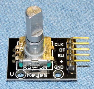
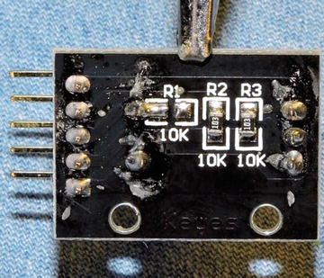
Figure 8-1. The Keyes YL-040 rotary encoder

It is also possible to buy the encoder switch by itself on eBay, but I don’t recommend it. The PCB adds considerable convenience for pennies more than the cost of the switch. But the main reason to buy the assembled PCB unit is to get a working switch. I have given up on buying good rotary switches by themselves from eBay. I suspect that many eBay rotary switch offerings, if not all, are factory rejects and floor sweepings.

The Switch

To help convince you of the need for buying quality, let’s take an inside look at how switches are constructed. Figure 8-2 illustrates the contact side of a switch assembly that I did an autopsy on.

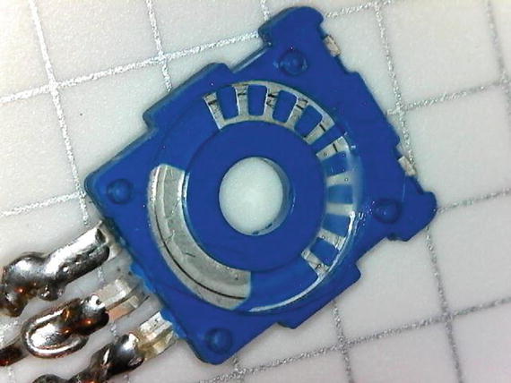
Figure 8-2. Contact side of the rotary encoder

Figure 8-2 shows that there is a contact pad (lower left) for the wiper arm. The top portion (right side of the figure) shows the other contact points. The smear seen there is some conductive grease. Figure 8-3 illustrates the wiper half of the assembly.

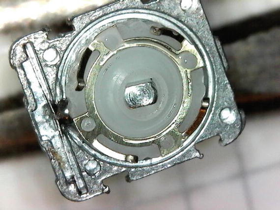
Figure 8-3. The wiper assembly of the rotary encoder

The photos illustrate the cheap nature of the rotary encoders’ construction. They must go through some sort of quality control at the factory, but it wouldn’t take much more than a bent wiper arm to render one faulty.

Figure 8-4 shows the KY-040 schematic without the optional push button switch. The units with the optional push switch have another connection labeled “SW” on the PCB. The return side of that switch connects to ground (GND).

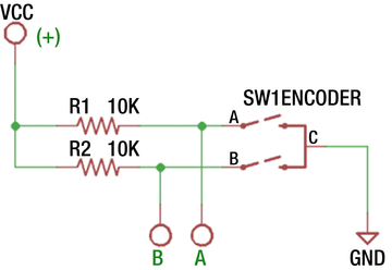
Figure 8-4. The KY-040 schematic (excluding optional push switch)

The schematic shown focuses on the rotary switches that connect switches A and B to the common point C. The KY-040 PCB includes two 10kΩ pull-up resistors so that when either switch is open, the host will read a high (1 bit). When the A or B switch is closed, this brings the signal level low (0 bit). Finally, note that the KY-040 PCB labels the connections as CLK and DT. According to reference [1], switch A is the CLK connection, while B is the DT connection. These specifics are unimportant to its operation.

Operation

The rotary encoder opens and closes switches A and B as you rotate the knob. As the shaft is turns, both switches alternate between on and off at the detents. The magic occurs in between the detents, however, allowing you to determine the direction of travel. Figure 8-5 illustrates this effect.

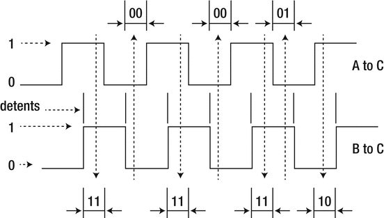
Figure 8-5. Rotary encoder signals

Starting from the first detent shown in Figure 8-5, switches A and B are open, reading 11 in bits (both read high). As the shaft is rotated toward the next detent, switches A and B become both closed (reading as 00). In between the detents however, you can see that switch A closes first (reading as 01), followed by switch B later (now reading 00). The timing of these changes allows you to determine the direction of travel. Had the shaft rotated in the reverse direction, switch B would close first (reading as 10), followed by A.

Voltage

As soon as you see the word Arduino, you should question whether the device is a 5V device because many Arduinos are 5V-based. For the KY-040 PCB, it doesn’t matter. Even though the reference [1] indicates that the supply voltage is 5 volts, it can be supplied the Raspberry Pi level of 3.3 volts instead. The rotary encoder is simply a pair of mechanical switches and has no voltage requirement.

Evaluation Circuit

The evaluation circuit can serve as an educational experiment and double as a test of the component. It is simple to wire up on a breadboard, and if the unit is working correctly, you will get a visual confirmation from the LEDs. Figure 8-6 illustrates the full circuit. The added components are shown at the left, consisting of resistors R ₃, R ₄ and the pair of LEDs.

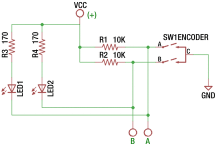
Figure 8-6. KY-040 evaluation circuit

The dropping resistors R ₃ and R ₄ are designed to limit the current flowing through the LEDs. Depending upon the LEDs you use, these should work fine at 3.3 or 5 volts. Assuming a forward voltage of about 1.8 volts for red LEDs and the circuit powered from 3.3 volts, this should result in approximately:

If you want to use less current for smaller LEDs, adjust the resistor higher than 170Ω.

Figure 8-7 illustrates my own simple breadboard test setup. You can see the dropping resistors R ₃ and R ₄ hiding behind the yellow LEDs that I had on hand at the moment. This test was performed using a power supply of 3.3 volts. The photo was taken with the shaft resting at a detent, which had both switches A and B closed, illuminating both LEDs.

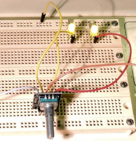
Figure 8-7. Evaluation test of the rotary encoder

When rotating the shaft, be sure to hold the shaft (a knob is recommended) securely so that you can see the individual LEDs turn on and off before the shaft snaps to the next detent. You should be able to see individual LED switching as you rotate.

If you see “skips” of LED on/off behavior for LED 1 and/or 2, this may indicate that you have a faulty switch. The only thing you can do for it is to replace it. But do check your wiring and connections carefully before you conclude that.

Interfacing to the Pi

Now it is time to interface this to the Raspberry Pi. Since the KY-040 PCB already provides the pull-up resistors, you only need to connect the + terminal to the Pi’s 3.3V supply and wire the A/CLK and B/DT connections to GPIO inputs. Don’t forget to connect GND to the Pi’s ground.

But before doing so, consider this: what kind of port are the GPIO pins you have selected at boot time? That is, what is their default configuration? If a particular GPIO is an output at boot time and if one or both of the rotary switches are closed, then you are short-circuiting the output until the port is reconfigured as an input. Given the amount of boot time, this could result in a damaged GPIO port.

Before hooking up GPIO ports to switches, you should do one of two things:

• Use GPIOs that are known to be inputs at boot time (and stay that way).

• Use isolation resistors to avoid damage when the GPIOs are outputs (best).

Using isolation resistors is highly recommended. By doing this, it won’t matter if the port is initially (or subsequently) configured as an output port. If your isolation resistor is chosen as 1kΩ (for example), the maximum output current will be limited to 3.3mA, which is too low to cause damage. Figure 8-8 illustrates the Pi hookup, using isolation resistors.

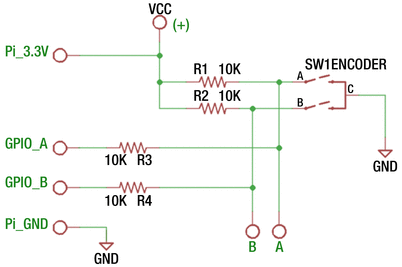
Figure 8-8. Safe hookup of the rotary switch to the Raspberry Pi

The schematic uses 10kΩ isolation resistors to hook up the rotary encoder to the Pi. If the selected GPIOs should ever be configured as outputs, the current will be limited to 0.33mA. Once the GPIOs are reconfigured by your application to be inputs, the readings will occur as if the resistors were not there. This happens because the CMOS inputs are driven mainly by voltage. The miniscule amount of current involved results in almost no voltage drop across the resistors.

Figure 8-9 shows a photo of the breadboard setup. An old knob was put onto the rotary controller to make it easier to rotate. In this experiment, the following GPIOs were used:

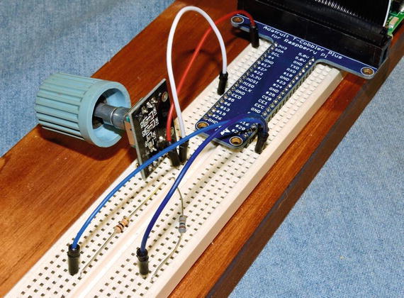
Figure 8-9. YL-040 rotary encoder hooked up to Raspberry Pi 3

• GPIO#20 was wired to CLK (via 10kΩ resistor)

• GPIO#21 was wired to DT (via 10kΩ resistor)

To verify that things are connected correctly, you can use the gp command to verify operation. Here you are testing GPIO #20 to see that it switches on and off:

$ gp -g20 -i -pu -m0
Monitoring..
000000 GPIO 20 = 1
000001 GPIO 20 = 0
000002 GPIO 20 = 1
000003 GPIO 20 = 0
000004 GPIO 20 = 1
000005 GPIO 20 = 0
...

Repeat the same test for GPIO #21.

$ gp -g21 -i -pu -m0
Monitoring..
000000 GPIO 21 = 0
000001 GPIO 21 = 1
000002 GPIO 21 = 0
000003 GPIO 21 = 1
000004 GPIO 21 = 0
000005 GPIO 21 = 1
000006 GPIO 21 = 0

Observe that the switch seems to change cleanly between 1 and 0 without any contact bounce. That may not always happen, however.

Experiment

As a simple programmed experiment, change to the software subdirectory YL-040. If you don’t see the executable yl040a, then type the make command to compile it now. With the circuit wired as in Figure 8-8, run the program yl040a and watch the session output as you turn the knob clockwise. Use Control-C to exit the program.

$ ./yl040a
00
10
11
01
00
^C

You should observe the general pattern shown in Table 8-1, perhaps starting at a different point. You should observe this sequence repeating as you rotate the control clockwise. If not, try counterclockwise. If the pattern shown here occurs in the reverse direction, simply exchange the connections for GPIO #20 and GPIO #21.

Note that the 00 and 11 patterns occur at the detents. The 10 and 01 patterns occur as you rotate from one detent position to the next. Rotating the knob in the reverse direction should yield a pattern like this:

$ ./yl040a
00
01
11
10
00
01
^C

Don’t worry if you see some upset in the sequence runs. There is likely to be some contact bounce that your next program will have to mitigate. The pattern however, should generally show what Table 8-2 illustrates.

From this, you see that rotation in one direction closes or opens a switch ahead of the other, offering information about rotational direction. There is still the problem of contact bounce, which you might have observed from your experiments. The next program will apply debouncing.

Experiment

Chapter 5 showed how software debouncing could be done. You’re going to apply that same technique in program yl040b for this experiment. Run the program and rotate the knob clockwise.

$ ./yl040b
00
10
11
01
00
10
11
01
00
10
11
01
00
10
11
01
00
10
11
^C

In this output, you can see the debounced sequence is faithful until the end. Despite this, it is possible that if you rotated the knob fast enough, there may have been discontinuities in the expected sequence. You’ll need to address this in the software.

Sequence Errors

Error handling in device driver software can be tricky. Let’s begin by looking at what can go wrong. Then let’s decide on an error recovery strategy. Here are events that could go astray:

• Debouncing was not effective enough, returning erratic events.

• The control was rotated faster than can be read and debounced.

• The control became defective or a connection was lost.

You’ll look at code at the end of the chapter, but program yl040b uses 4 bits of shift register to debounce the rotary input. Switch events from a rotary control can occur more rapidly than a push button, so a short debounce period is used, lasting about 68 μsec × 4 = 272 μsec. If you take too long, the control can advance to the next point before you stabilize a reading.

When the control is rotated rapidly, you can lose switch events because the Pi was too busy or because the events occurred too quickly. When this happens, you can have readings appear out of sequence. If you read 00 immediately followed by 11, you do not know the direction of the travel. Lost or mangled events also occur when the control becomes faulty.

So, what do you do when an event occurs out of sequence? Do you:

• Ignore the error and wait for the control to reach one of the expected two states?

• Reset your state to the currently read one?

The class RotarySwitch defined in files rotary.hpp and rotary.cpp has taken the first approach. If it encounters an invalid state, it simply returns a “no change” event. Eventually when the control is rotated far enough, it will match one of the two expected next states. The second approach would avoid further lost events but may register events in the wrong direction occasionally.

Experiment

Program yl040c was written to allow you to test-drive the rotary control with a counter. Run the program with the control ready.

$ ./yl040c
Monitoring rotary control:
Step +1, Count 1
Step +1, Count 2
Step +1, Count 3
Step +1, Count 4
Step +1, Count 5
Step -1, Count 4
Step -1, Count 3
Step -1, Count 2
Step -1, Count 1
Step -1, Count 0
Step -1, Count -1
Step -1, Count -2
Step -1, Count -3
Step +1, Count -2
Step +1, Count -1
Step +1, Count 0
^C

The program clearly states the direction of the step as clockwise (+1) or counterclockwise (-1) and reports the affected counter. The counter is taken up to 5 by a clockwise motion and taken back to -3 in a counterclockwise motion and then clockwise again to return to 0. When your control is working properly, this will be an effortless exercise.

FM Dial 1

While your rotary control seems to work nicely, it may not be convenient enough in its current form. To illustrate this, let’s simulate the FM stereo tuner knob with the rotary control. Run the program fm1 with the control ready. Try tuning from end to end of the FM dial (the program starts you in the middle).

$ ./fm1
FM Dial with NO Flywheel Effect.
100.0 MHz
100.1 MHz
100.2 MHz
100.3 MHz
100.4 MHz
100.5 MHz
100.6 MHz
100.7 MHz
100.8 MHz
100.9 MHz
101.0 MHz
101.1 MHz
101.2 MHz
101.3 MHz
101.2 MHz
101.1 MHz
101.0 MHz
100.9 MHz
100.8 MHz
100.7 MHz
100.6 MHz
100.5 MHz
100.4 MHz
100.3 MHz
100.2 MHz
100.1 MHz
100.0 MHz
 99.9 MHz
 99.8 MHz
 99.7 MHz
 99.6 MHz
 99.5 MHz
 99.4 MHz
 99.3 MHz
 99.2 MHz
 99.1 MHz
 99.0 MHz
 99.1 MHz
^C

How convenient was it to go from 100.0MHz down to 99.1MHz? Did you have to twist the knob a lot? To save rotational effort, many electronic controls simulate a “flywheel effect.”

The program fm1 uses the RotarySwitch class, which responds in a simple linear fashion to the rotary encoder. If the control clicks once to the right, it responds by incrementing the count by 1. If it clicks counterclockwise, the counter is decremented by 1 instead. You’ll look at code for this at the end of this chapter.

Spin a bicycle wheel, and it continues to rotate after you stop and watch. Friction causes the rotation to slow and eventually stop. This is flywheel action, and it is convenient to duplicate this in a control. Some high-end stereo and ham radio gear have heavy knobs in place so that they continue to rotate if you spin them fast enough.

FM Dial 2

Let’s repeat the last experiment with the program fm2. In the following example, the dial was turned clockwise slowly at first. Then a more rapid twist was given, and the dial shot up to about 102.0MHz. One more rapid counterclockwise twist took the frequency down to 98.8MHz.

$ ./fm2
FM Dial with Flywheel Effect.
100.0 MHz
100.1 MHz
100.2 MHz
100.3 MHz
100.4 MHz
100.5 MHz
100.6 MHz
100.8 MHz
101.0 MHz
101.2 MHz
101.4 MHz
101.6 MHz
101.7 MHz
101.8 MHz
101.9 MHz
102.0 MHz
101.9 MHz
101.8 MHz
101.7 MHz
101.6 MHz
101.5 MHz
101.3 MHz
101.0 MHz
100.8 MHz
100.6 MHz
100.2 MHz
 99.8 MHz
 99.5 MHz
 99.3 MHz
 99.1 MHz
 98.9 MHz
 98.8 MHz
 98.7 MHz
 98.6 MHz
 98.7 MHz
 98.8 MHz
 98.9 MHz
 99.0 MHz

With a more vigorous twist of the knob, you can quickly go from one end of the dial to the other. Yet, when rotation speeds are reduced, you have full control with fine adjustments. It is important to retain this later quality.

The following session output demonstrates some vigorous tuning changes:

$ ./fm2
FM Dial with Flywheel Effect.
100.0 MHz
100.1 MHz
100.2 MHz
100.3 MHz
100.4 MHz
100.5 MHz
100.8 MHz
101.4 MHz
102.3 MHz
103.4 MHz
104.6 MHz
105.8 MHz
107.2 MHz
107.9 MHz
107.9 MHz
107.9 MHz
107.9 MHz
107.9 MHz
107.9 MHz
107.8 MHz
107.7 MHz
107.6 MHz
107.5 MHz
107.4 MHz
107.2 MHz
106.7 MHz
105.8 MHz
104.3 MHz
102.2 MHz
 99.8 MHz
 97.2 MHz
 94.6 MHz
 91.9 MHz
 89.2 MHz
 88.1 MHz
 88.1 MHz
 88.1 MHz
 88.1 MHz

Class Switch

To keep the programs simple, I’ve built up the programs using C++ classes. The GPIO class is from the librpi2 library, which you should have installed already (see Chapter 1). This gives you convenient direct access to the GPIO ports.

Listing 8-1 illustrates the Switch class definition. This functions well as the contract between the end user and the implementation of the class. Aside from instantiating the Switch class in the user program, the only method call that is of interest is the read() method, which reads from the GPIO port and debounces the signal.

Listing 8-1. The Switch Class for Handling Rotary Encoder Contacts and Debouncing in switch.hpp

009 /*
010  * Class for a single switch
011  */
012 class Switch {
013     GPIO&          gpio;   // GPIO Access
014     int            gport;  // GPIO Port #
015     unsigned       mask;   // Debounce mask
016     unsigned       shiftr; // Debouncing shift register
017     unsigned       state;  // Current debounced state
018
019 public: Switch(GPIO& gpio,int port,unsigned mask=0xF);
020     unsigned read();       // Read debounced
021 };

Listing 8-2 shows the constructor for this class. The reference (argument agpio) to the caller’s instance of the GPIO class is saved in the Switch class for later use in line 010 (as gpio). The GPIO port chosen for this switch is indicated in aport and saved in gport. The value of amask defaults to the value of 0x0F, which specifies that 4 bits are to be used for debouncing. You can reduce the number of bits to 3 bits by specifying the value of 0x07.

Listing 8-2. The Switch Class Constructor Code in switch.cpp

006 /*
007  * Single switch class, with debounce:
008  */
009 Switch::Switch(GPIO& agpio,int aport,unsigned amask)
010 : gpio(agpio), gport(aport), mask(amask) {
011
012     shiftr = 0;
013     state = 0;
014
015     // Configure GPIO port as input
016     gpio.configure(gport,GPIO::Input);
017     assert(!gpio.get_error());
018
019     // Configure GPIO port with pull-up
020     gpio.configure(gport,GPIO::Up);
021     assert(!gpio.get_error());
022 }

The shift register for debouncing (shiftr) is initialized to 0 in line 012, and the variable state is initialized to 0 also. Line 016 configures the specified GPIO port as an input and activates its pull-up resistor in line 020.

The assert() macros used will cause an abort if the expressions provided ever evaluate as false. These give the programmer the assurance that nothing unexpected has happened. They can be disabled by defining the macro NDEBUG at compile time, if you like. The cost of these is low, so I usually leave them compiled in.

Listing 8-3 illustrates the code for reading the switch and debouncing the contacts. The algorithm used is the same procedure as described in Chapter 5.

Listing 8-3. The Switch::read() Method for Debouncing Contacts in switch.cpp

024 /*
025  * Read debounced switch state:
026  */
027 unsigned
028 Switch::read() {
029     unsigned b = gpio.read(gport);
030     unsigned s;
031
032     shiftr = (shiftr << 1) | (b & 1);
033     s = shiftr & mask;
034
035     if ( s != mask && s != 0x00 )
036            return state;   // Bouncing: return state
037     if ( s == state )
038             return state;  // No change
039     state = shiftr & 1;    // Set new state
040     return state;
041 }

The Switch class provides input and debouncing for only one contact. To make a rotary control, you need to debounce two switches. For that, you define the RotarySwitch class shown in Listing 8-4.

Listing 8-4. The RotarySwitch Class for Debouncing and Reading in rotary.hpp

008 /*
009  * Class for a (pair) rotary switch:
010  */
011 class RotarySwitch {
012     Switch         clk;    // CLK pin
013     Switch         dt;     // DT pin
014     unsigned       index;  // Index into states[]
015 protected:
016     unsigned read_pair();  // Read (CLK << 1) | DT
017
018 public: RotarySwitch(GPIO& gpio,int clk,int dt,unsigned mask=0xF);
019     int read();            // Returns +1, 0 or -1
020 };

In the RotarySwitch class, notice how the two switch contacts are handled by two Switch class instances named clk and dt (lines 012 and 013). Line 014 declares a variable index, which will be described shortly. The class method read_pair() is declared in the protected region so that when using class inheritance, you will have access to it (line 016). The constructor in line 018 is almost the same as Switch, except that you have two GPIO numbers provided for clk and dt.

Listing 8-5 shows the read_pair() method code. It reads a bit from switches clk and dt and returns them as a pair of bits for convenience. Lumping them together in this way provides some programming convenience.

Listing 8-5. RotarySwitch::read_pair() Method in rotary.cpp

029 /*
030  * Protected: Read switch pair
031  */
032 unsigned
033 RotarySwitch::read_pair() {
034   return (clk.read() << 1) | dt.read();
035 }

Listing 8-6 shows the more interesting code. To read the encoder, a small table is used, declared in lines 008 and 009. These identify the next bit pairs expected when rotation is progressing clockwise.

Listing 8-6. The RotarySwitch::read() Method for Interpreting the Rotary Encoder in rotary.cpp

05 /*
006  * State array for CLK & DT switch settings:
007  */
008 static unsigned states[4] =
009     { 0b00, 0b10, 0b11, 0b01 };
010
...
038 /*
039  * Read rotary switch:
040  *
041  * RETURNS:
042  * +1      Rotated clockwise
043  *  0      No change
044  * -1      Rotated counter-clockwise
045  */
046 int
047 RotarySwitch::read() {
048     unsigned pair = read_pair();
049     unsigned cw = (index + 1) % 4;
050     unsigned ccw = (index + 3) % 4;
051
052     if ( pair != states[index] ) {
053             // State has changed
054             if ( pair == states[cw] ) {
055                    index = cw;
056                    return (pair == 0b11 || pair == 0b00) ? +1 : 0;
057             } else if ( pair == states[ccw] ) {
058                    index = ccw;
059                    return (pair == 0b11 || pair == 0b00) ? -1 : 0;
060             }
061    }
062
063    return 0;        // No change
064 }

As the comments document (lines 041 to 044), the RotarySwitch::read() method returns a signed value.

• +1 when the control has rotated clockwise

• -1 if in the reverse

• 0 if there was no event to report

The first operation is to read from the pair of switches (line 048). This bit pair is debounced thanks to the work of the Switch class that was used to manage them. The values cw and ccw are the computed next index values into array states for clockwise and counterclockwise (lines 049 and 050).

Line 052 checks to see whether the value read (variable pair) has changed from the last time. If so, an event has happened, and line 054 tests to see whether you went clockwise. If so, the value of index is updated in line 055 and a +1 or 0 is returned. The +1 is returned, however, only if the control is now at one of the detent positions where pair reads as 0b00 or 0b11. Otherwise, you pretend that nothing happened by returning 0. Lines 057 to 059 perform the same function for counterclockwise. Failing all else, line 063 returns 0 to indicate that nothing interesting happened.

Listing 8-7 shows how the class Flywheel inherits from class RotarySwitch. This allows you to leverage what you’ve already built, while adding the flywheel effect on top. The constructor in line 019 for Flywheel is the same as for RotarySwitch. Like before, the Flywheel::read() method returns the same values.

Listing 8-7. Class Flywheel for Rotary Control with Flywheel Effect, in flywheel.hpp

011 /*
012  * Class for a (pair) Rotary switch:
013  */
014 class Flywheel : public RotarySwitch {
015     timespec       t0;     // Time of last motion
016     double         ival;   // Last interval time
017     int            lastr;  // Last returned value r
018
019 public: Flywheel(GPIO& gpio,int clk,int dt,unsigned mask=0xF);
020     int read();            // Returns +1, 0 or -1
021 };

To implement the Flywheel class, you need a fine set of timing functions. Listing 8-8 shows some local functions that are used by the class. The function get_time() is used to get time with nanosecond precision. It should be understood, however, that the time returned in the structure timespec may not be that accurate but is provided in seconds (member tv_sec) and nanoseconds (member tv_nsec).

Listing 8-8. The Local Static Functions Used by the Flywheel Implementation, in flywheel.cpp

009 static inline void
010 get_time(timespec& tv) {
011   int rc = clock_gettime(CLOCK_MONOTONIC,&tv);
012   assert(!rc);
013 }
014
015 static inline double
016 as_double(const timespec& tv) {
017   return double(tv.tv_sec) + double(tv.tv_nsec) / 1000000000.0;
018 }
019
020 static inline double
021 timediff(const timespec& t0,const timespec& t1) {
022   double d0 = as_double(t0), d1 = as_double(t1);
023
024   return d1 - d0;
025 }
026
027 Flywheel::Flywheel(GPIO& agpio,int aclk,int adt,unsigned amask)
028 : RotarySwitch(agpio,aclk,adt,amask) {
029
030   get_time(t0);
031   lastr = 0;
032 };

The function as_double() in lines 015 to 018 convert the timespec value into a double value, which is more convenient to compute with. The routine timediff() in lines 020 to 025 compute the time difference in seconds.

The constructor in lines 027 to 032 initializes the inherited RotarySwitch class (line 028) and initializes t0 with a start time.

Listing 8-9 is the main star of this chapter, illustrating the extra code used to implement the flywheel effect. Line 035 replaces the RotarySwitch::read() method for this class with new code and tricks.

Listing 8-9. The Meat of the Flywheel Class in flywheel.cpp

034 int
035 Flywheel::read() {
036     static const double speed = 15.0; // Lower values change faster
037     timespec t1;                   // Time now
038     double diff, rate;             // Difference, rate
039     int r, m = 1;                  // Return r, m multiple
040
041     r = RotarySwitch::read();       // Get reading (debounced)
042     get_time(t1);                   // Now
043     diff = timediff(t0,t1);         // Diff in seconds
044
045     if ( r != 0 ) {                // Got a click event
046             lastr = r;             // Save the event type
047             ival = ( ival * 0.75 + diff * 1.25 ) / 2.0 * 1.10;
048             if ( ival < 1.0 && ival > 0.00001 ) {
049                    rate = 1.0 / ival;
050             } else rate = 0.0;
051             t0 = t1;
052             if ( speed > 0.0 )
053                    m = rate / speed;
054    } else if ( diff > ival && ival >= 0.000001 ) {
055            rate = 1.0 / ival;      // Compute a rate
056            if ( rate > 15.0 ) {
057                    if ( speed > 0.0 )
058                            m = rate / speed;
059                    ival *= 1.2;    // Increase interval
060                    t0 = t1;
061                    r = lastr;      // Return last r
062            }
063     }
064
065     return m > 0 ? r * m : r;
066 }

Line 041 uses the original RotarySwitch::read() call to read the value of +1, 0, or -1 depending upon the rotary control. But the Flywheel version of read() will perform some additional processing.

Line 042 assigns the current time in nanoseconds to t1. Using the start time t0, the elapsed time from the last event is computed in line 043 (variable diff). This difference in time is a floating-point value in seconds but includes the fractional difference in nanoseconds. If the control has been sitting idle for a long time, this difference may be very long for the first time (perhaps minutes or hours). However, successive events will have time differences of perhaps of 10 milliseconds.

Line 045 tests to see whether you got an event in variable r. If there was rotation, r will be nonzero. The rotation event is recorded for later use in line 046 (variable lastr). Then a weighted average is computed from the prior interval and current difference in line 047 (stored in variable ival). An additional 10 percent is added to the value by multiplying by 1.10. The rationale for this adjustment will be revealed shortly, including why lines 048 to 053 compute a rate value and a multiple m.

Lines 045 to 053 just described operate when there is a rotational event—either the control has clicked over, clockwise or clockwise. But what happens after quickly rotating the knob and releasing it? Or slowing down?

When there is no rotational event in line 045, control passes to line 054 to test whether the current time difference (diff) is greater than the last computed interval ival. Recall that the weighted value of ival had 10 percent added to it (at the end of line 047). As the rotational rate increases, the time difference between events gets smaller (diff). So, as long as this time interval decreases or remains about the same, the generated flywheel events are suppressed. In fact, the rate of rotation would have to drop below 10 percent of the current weighted average before the flywheeling applies. By doing this, expected events that occur on time are handled normally. Only when expected next events are late do you consider synthesizing events in the flywheeling code.

Line 054 also insists that the last weighted interval time (ival) is greater than 0.000001. This is a rate-limiting action on the flywheeling effect. Line 055 computes a rate, which is the inverse of time interval (ival). Only when the rate rises above 15.0 do you synthesize more flywheel events (line 056). The variable speed is hard-coded with the value 15.0 (line 036). It is used to compute the multiple m from the rate using division (lines 053 and 058). If you change the value of speed to zero, there will be no multiplying effect.

The effect of the multiple of m is to increase the value returned from a simple +1 to, say, a +8, when the rotational rate is high. This applies to line 065. When the rotational rate slows, the multiple has less effect, and the control responds in smaller increments.

In the flywheeling section in line 059, you compute a next interval time (ival). Here the interval time has 20 percent added to it so that it slows and becomes less likely to synthesize another event. This reduces the next rate calculation in line 056. As ival is increased, eventually the rate value drops below 15.0 and then ceases to synthesize any more events. Lines 060 and 061 reset the timer t0 and set the returned r to the lastr value saved. Line 065 brings it all together by applying multiple m and r.

Main Routine

To knit this all together, let’s review the main program for fm2.cpp, which uses the Flywheel class. Because the tricky stuff is located inside the class implementation code, the main programs used in this chapter are essentially the same. Listing 8-10 presents fm2.cpp.

Listing 8-10. The Main Program for fm2.cpp

012 #include "flywheel.hpp"
013
014 /*
015  * Main test program:
016  */
017 int
018 main(int argc,char **argv) {
019     GPIO gpio;             // GPIO access object
020     int rc, counter = 1000;
021
022     // Check initialization of GPIO class:
023     if ( (rc = gpio.get_error()) != 0 ) {
024             fprintf(stderr,"%s: starting gpio (sudo?)\n",strerror(rc));
025            exit(1);
026     }
027
028     puts("FM Dial with Flywheel Effect.");
029     printf("%5.1lf MHz\n",double(counter)/10.0);
030
031     // Instantiate our rotary switch:
032     Flywheel rsw(gpio,20,21);
033
034     // Loop reading rotary switch for changes:
035     for (;;) {
036            rc = rsw.read();
037             if ( rc != 0 ) {
038                    // Position changed:
039                    counter += rc;
040                    if ( counter < 881 )
041                            counter = 881;
042                    else if ( counter > 1079 )
043                            counter = 1079;
044                    printf("%5.1lf MHz\n",double(counter)/10.0);
045              } else {
046                    // No position change
047                    usleep(1);
048              }
049     }
050
051     return 0;
052 }

The GPIO class is instantiated as gpio in line 019, and errors are checked in lines 023 to 026. The Flywheel class is instantiated in line 032, with the gpio class passed in as part of the constructor.

The main loop consists of lines 035 to 049. If you read a rotational event, then lines 038 to 044 are executed. Otherwise, a delay of usleep(1) is performed in line 047. On the Raspberry Pi 3 this takes about 68μsec and serves only to pass control to some other process needing the CPU. According to htop(1), this uses about 27 percent of one core. You can increase the sleep time to something above 68μsec to reduce this overhead. But if you overdo the delay, the control will become less responsive.

Summary

In this chapter you discovered rotary encoders and applied the principles of contact debouncing to a reliable read position. From this foundation, you saw code to sense rotary motion and apply flywheeling to make the control more effective. This refashions the humble rotary control as a powerful user input for the Raspberry Pi.

Bibliography

1. “Keyes KY-040 Arduino Rotary Encoder User Manual.” Henrys Bench. 2015. Accessed August 13, 2016. < http://henrysbench.capnfatz.com/henrys-bench/arduino-sensors-and-input/keyes-ky-040-arduino-rotary-encoder-user-manual/ >.