Table of Contents for
Machine Learning for Hackers
 Machine Learning for Hackers
Published by
O'Reilly Media, Inc., 2012
Machine Learning for Hackers
Published by
O'Reilly Media, Inc., 2012
- Cover
- O'Reilly Strata Conference
- Machine Learning for Hackers
- Preface
- 1. Using R
- 2. Data Exploration
- 3. Classification: Spam Filtering
- 4. Ranking: Priority Inbox
- 5. Regression: Predicting Page Views
- 6. Regularization: Text Regression
- 7. Optimization: Breaking Codes
- 8. PCA: Building a Market Index
- 9. MDS: Visually Exploring US Senator Similarity
- 10. kNN: Recommendation Systems
- 11. Analyzing Social Graphs
- 12. Model Comparison
- Works Cited
- Index
- About the Authors
- Colophon
- Copyright
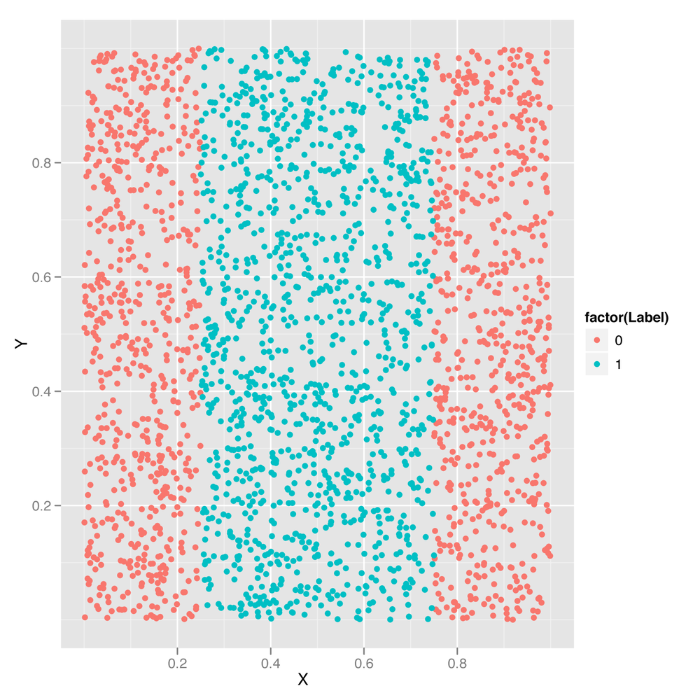
In Chapter 3, we introduced the idea of decision boundaries and noted that problems in which the decision boundary isn’t linear pose a problem for simple classification algorithms. In Chapter 6, we showed you how to perform logistic regression, a classification algorithm that works by constructing a linear decision boundary. And in both chapters, we promised to describe a technique called the kernel trick that could be used to solve problems with nonlinear decision boundaries. Let’s deliver on that promise by introducing a new classification algorithm called the support vector machine (SVM for short), which allows you to use multiple different kernels to find nonlinear decision boundaries. We’ll use an SVM to classify points from a data set with a nonlinear decision boundary. Specifically, we’ll work with the data set shown in Figure 12-1.
Looking at this data set, it should be clear that the points from
Class 0 are on the periphery, whereas points from Class 1 are in the
center of the plot. This sort of nonlinear decision boundary can’t be
discovered using a simple classification algorithm like the logistic
regression algorithm we described in Chapter 6. Let’s demonstrate that by trying to use logistic regression
through the glm function. We’ll then look into the reason
why logistic regression fails.
df <- read.csv('data/df.csv')

logit.fit <- glm(Label ~ X + Y,
                 family = binomial(link = 'logit'),
                 data = df)

logit.predictions <- ifelse(predict(logit.fit) > 0, 1, 0)

mean(with(df, logit.predictions == Label))
#[1] 0.5156
As you can see, we’ve correctly predicted the class of only 52% of the data. But we could do exactly this well by predicting that every data point belongs to Class 0:
mean(with(df, 0 == Label))
#[1] 0.5156
In short, the logistic regression model (and the linear decision boundary it finds) is completely useless. It makes the same predictions as a model with no information beyond the fact that Class 0 occurs more often than Class 1, and so should be used as a prediction in the absence of all other information.
So how can we do better? As you’ll see in a moment, the SVM
provides a trivial way to outperform logistic regression. Before we
describe how it does this, let’s just show you that it works as a
black-box algorithm that produces useful answers. To do so, we’ll use the e1071 package, which
provides a function svm that is just as easy to use as
glm:
library('e1071')

svm.fit <- svm(Label ~ X + Y, data = df)
svm.predictions <- ifelse(predict(svm.fit) > 0, 1, 0)
mean(with(df, svm.predictions == Label))
#[1] 0.7204
Here we’ve clearly done better than logistic regression just by switching to SVMs. How is the SVM doing this?
The first way to gain insight into the superior performance of the SVM is to plot its predictions versus those from a logistic regression:
df <- cbind(df,
            data.frame(Logit = ifelse(predict(logit.fit) > 0, 1, 0),
                       SVM = ifelse(predict(svm.fit) > 0, 1, 0)))

predictions <- melt(df, id.vars = c('X', 'Y'))

ggplot(predictions, aes(x = X, y = Y, color = factor(value))) +
  geom_point() +
  facet_grid(variable ~ .)
Here we’ve added the logistic regression predictions and the
SVM predictions to the raw data set. Then we use the melt
function to build up a data set that’s easier to work with for plotting
purposes, and we store this new data set in a data frame called predictions. We then plot the
ground truth labels along with the logit and SVM predictions in the
faceted plot shown in Figure 12-2.
Once we’ve done this, it becomes obvious that the logistic regression is useless because it puts the decision boundary outside of the data set, while the ground truth data in the top row clearly has a band of entries for Class 1 in the center. The SVM is able to capture this band structure, even though it makes odd predictions near the furthest boundaries of the data set.
So now we’ve seen that the SVM produces, as promised, a nonlinear decision boundary. But how does it do that? The answer is that the SVM uses the kernel trick. Using a mathematical transformation, it moves the original data set into a new mathematical space in which the decision boundary is easy to describe. Because this transformation depends only on a simple computation involving “kernels,” this technique is called the kernel trick.
Describing the mathematics of the kernel trick is nontrivial, but
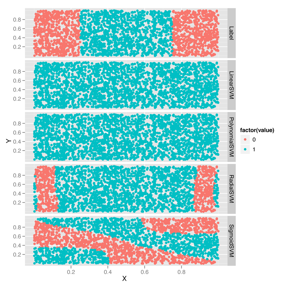
it’s easy to gain some intuition by testing out different kernels.
This is easy because the SVM function has a parameter called
kernel that can be set to one of four values: linear,
polynomial, radial, and sigmoid. To get a feel for how these kernels
work, let’s try using all of them to generate predictions and then plot
the predictions:
df <- df[, c('X', 'Y', 'Label')]

linear.svm.fit <- svm(Label ~ X + Y, data = df, kernel = 'linear')
with(df, mean(Label == ifelse(predict(linear.svm.fit) > 0, 1, 0)))

polynomial.svm.fit <- svm(Label ~ X + Y, data = df, kernel = 'polynomial')
with(df, mean(Label == ifelse(predict(polynomial.svm.fit) > 0, 1, 0)))

radial.svm.fit <- svm(Label ~ X + Y, data = df, kernel = 'radial')
with(df, mean(Label == ifelse(predict(radial.svm.fit) > 0, 1, 0)))

sigmoid.svm.fit <- svm(Label ~ X + Y, data = df, kernel = 'sigmoid')
with(df, mean(Label == ifelse(predict(sigmoid.svm.fit) > 0, 1, 0)))

df <- cbind(df,
            data.frame(LinearSVM = ifelse(predict(linear.svm.fit) > 0, 1, 0),
                       PolynomialSVM = ifelse(predict(polynomial.svm.fit) > 0, 1, 0),
                       RadialSVM = ifelse(predict(radial.svm.fit) > 0, 1, 0),
                       SigmoidSVM = ifelse(predict(sigmoid.svm.fit) > 0, 1, 0)))

predictions <- melt(df, id.vars = c('X', 'Y'))

ggplot(predictions, aes(x = X, y = Y, color = factor(value))) +
  geom_point() +
  facet_grid(variable ~ .)
As you can see from Figure 12-3, the linear and polynomial kernels look more or less like logistic regression. In contrast, the radial kernel gives us a decision boundary somewhat like the ground truth boundary. And the sigmoid kernel gives us a very complex and strange decision boundary.
You should generate some of your own data sets and play around with these four kernels to build up your intuition for how they work. After you’ve done that, you may suspect that the SVM could make much better predictions than it seems to do out of the box. This is true. The SVM comes with a set of hyperparameters that are not set to useful values by default, and getting the best predictions from the model requires tuning these hyperparameters. Let’s describe the major hyperparameters and see how tuning them improves our model’s performance.
The first hyperparameter you can work with is the degree of
the polynomial used by the polynomial kernel. You can change this by
setting the value of degree when calling svm.
Let’s see how this hyperparameter works with four simple
examples:
polynomial.degree3.svm.fit <- svm(Label ~ X + Y,
data = df,
kernel = 'polynomial',
degree = 3)
with(df, mean(Label != ifelse(predict(polynomial.degree3.svm.fit) > 0, 1, 0)))
#[1] 0.5156
polynomial.degree5.svm.fit <- svm(Label ~ X + Y,
data = df,
kernel = 'polynomial',
degree = 5)
with(df, mean(Label != ifelse(predict(polynomial.degree5.svm.fit) > 0, 1, 0)))
#[1] 0.5156
polynomial.degree10.svm.fit <- svm(Label ~ X + Y,
data = df,
kernel = 'polynomial',
degree = 10)
with(df, mean(Label != ifelse(predict(polynomial.degree10.svm.fit) > 0, 1, 0)))
#[1] 0.4388
polynomial.degree12.svm.fit <- svm(Label ~ X + Y,
data = df,
kernel = 'polynomial',
degree = 12)
with(df, mean(Label != ifelse(predict(polynomial.degree12.svm.fit) > 0, 1, 0)))
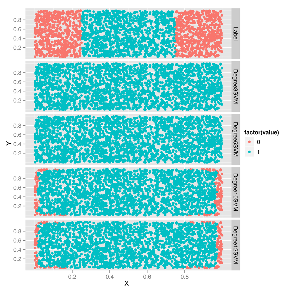
#[1] 0.4464Here we can see that setting degree to 3 or 5 doesn’t
have any effect on the quality of the model’s predictions. (It’s worth
noting that the default value of degree is 3.) But setting
degree to 10 or 12 does have an effect. To see what’s
happening, let’s plot out the decision boundaries again:
df <- df[, c('X', 'Y', 'Label')]

df <- cbind(df,
            data.frame(Degree3SVM = ifelse(predict(polynomial.degree3.svm.fit) > 0,
                                           1,
                                           0),
                       Degree5SVM = ifelse(predict(polynomial.degree5.svm.fit) > 0,
                                           1,
                                           0),
                       Degree10SVM = ifelse(predict(polynomial.degree10.svm.fit) > 0,
                                            1,
                                            0),
                       Degree12SVM = ifelse(predict(polynomial.degree12.svm.fit) > 0,
                                            1,
                                            0)))

predictions <- melt(df, id.vars = c('X', 'Y'))

ggplot(predictions, aes(x = X, y = Y, color = factor(value))) +
  geom_point() +
  facet_grid(variable ~ .)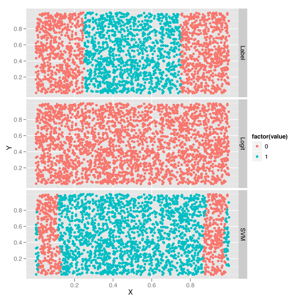
Looking at the predictions shown in Figure 12-4, it’s clear that using a
larger degree improves the quality of the predictions, though it does so
in a hackish way that’s not really mimicking the structure of the data.
And, as you’ll notice, the model-fitting step becomes slower and slower
as the degree increases. And finally, the same overfitting problems we
saw in Chapter 6 with polynomial
regression will creep up. For that reason, you should always use
cross-validation to experiment with setting the degree
hyperparameter in applications that use SVMs with polynomial kernels.
Although there’s no doubt that SVMs with polynomial kernels are a
valuable tool to have in your toolkit, they can’t be guaranteed to work
well without some effort and thinking on your part.
After playing with the degree hyperparameter for
the polynomial kernel, let’s try out the cost
hyperparameter, which is used with all of the possible SVM kernels. To
see the effect of changing cost, we’ll use a radial kernel
and try four different cost settings. To change things up,
we’ll also stop counting errors and start seeing how many data points we
predict correctly, as we’re ultimately interested in seeing how good the
best model is and not how bad the worst model is. The following shows
the code for this exploration of the cost parameter:
radial.cost1.svm.fit <- svm(Label ~ X + Y,
                            data = df,
                            kernel = 'radial',
                            cost = 1)
with(df, mean(Label == ifelse(predict(radial.cost1.svm.fit) > 0, 1, 0)))
#[1] 0.7204

radial.cost2.svm.fit <- svm(Label ~ X + Y,
                            data = df,
                            kernel = 'radial',
                            cost = 2)
with(df, mean(Label == ifelse(predict(radial.cost2.svm.fit) > 0, 1, 0)))
#[1] 0.7052

radial.cost3.svm.fit <- svm(Label ~ X + Y,
                            data = df,
                            kernel = 'radial',
                            cost = 3)
with(df, mean(Label == ifelse(predict(radial.cost3.svm.fit) > 0, 1, 0)))
#[1] 0.6996

radial.cost4.svm.fit <- svm(Label ~ X + Y,
                            data = df,
                            kernel = 'radial',
                            cost = 4)
with(df, mean(Label == ifelse(predict(radial.cost4.svm.fit) > 0, 1, 0)))
#[1] 0.694
As you can see, increasing the cost parameter makes
the model progressively fit more and more poorly. That’s because the cost is a regularization
hyperparameter like the lambda parameter we described in
Chapter 6, and increasing it
will always make the model fit the training data less tightly. Of
course, this increase in regularization can improve your model’s
performance on test data, so you should always see what value of
cost most improves your test performance using
cross-validation.
To get some insight into what’s happening in terms of the fitted model, let’s look at the predictions graphically in Figure 12-5:
df <- df[, c('X', 'Y', 'Label')]

df <- cbind(df,
            data.frame(Cost1SVM = ifelse(predict(radial.cost1.svm.fit) > 0, 1, 0),
                       Cost2SVM = ifelse(predict(radial.cost2.svm.fit) > 0, 1, 0),
                       Cost3SVM = ifelse(predict(radial.cost3.svm.fit) > 0, 1, 0),
                       Cost4SVM = ifelse(predict(radial.cost4.svm.fit) > 0, 1, 0)))

predictions <- melt(df, id.vars = c('X', 'Y'))

ggplot(predictions, aes(x = X, y = Y, color = factor(value))) +
  geom_point() +
  facet_grid(variable ~ .)
The changes induced by the cost parameter are quite
subtle, but can be seen on the periphery of the data set shown in Figure 12-5. As the cost goes up,
the boundaries created by the radial kernel become more and
more linear.
Having looked at the cost parameter, we’ll conclude
our SVM hyperparameter experiments by playing around with the
gamma hyperparameter. For testing purposes, we’ll observe
its effects on a sigmoid kernel by testing out four different
gamma values:
sigmoid.gamma1.svm.fit <- svm(Label ~ X + Y,
                              data = df,
                              kernel = 'sigmoid',
                              gamma = 1)
with(df, mean(Label == ifelse(predict(sigmoid.gamma1.svm.fit) > 0, 1, 0)))
#[1] 0.478

sigmoid.gamma2.svm.fit <- svm(Label ~ X + Y,
                              data = df,
                              kernel = 'sigmoid',
                              gamma = 2)
with(df, mean(Label == ifelse(predict(sigmoid.gamma2.svm.fit) > 0, 1, 0)))
#[1] 0.4824

sigmoid.gamma3.svm.fit <- svm(Label ~ X + Y,
                              data = df,
                              kernel = 'sigmoid',
                              gamma = 3)
with(df, mean(Label == ifelse(predict(sigmoid.gamma3.svm.fit) > 0, 1, 0)))
#[1] 0.4816

sigmoid.gamma4.svm.fit <- svm(Label ~ X + Y,
                              data = df,
                              kernel = 'sigmoid',
                              gamma = 4)
with(df, mean(Label == ifelse(predict(sigmoid.gamma4.svm.fit) > 0, 1, 0)))
#[1] 0.4824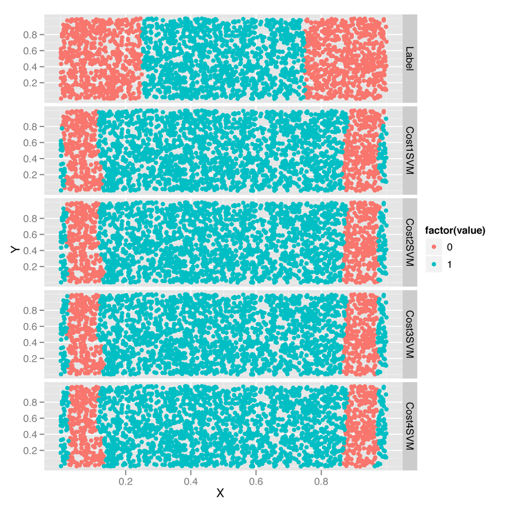
Every time we increase gamma, the model does a little
better. To get a sense for the source of that improvement, let’s turn to
graphical diagnostics of the predictions:
df <- df[, c('X', 'Y', 'Label')]

df <- cbind(df,
            data.frame(Gamma1SVM = ifelse(predict(sigmoid.gamma1.svm.fit) > 0, 1, 0),
                       Gamma2SVM = ifelse(predict(sigmoid.gamma2.svm.fit) > 0, 1, 0),
                       Gamma3SVM = ifelse(predict(sigmoid.gamma3.svm.fit) > 0, 1, 0),
                       Gamma4SVM = ifelse(predict(sigmoid.gamma4.svm.fit) > 0, 1, 0)))

predictions <- melt(df, id.vars = c('X', 'Y'))

ggplot(predictions, aes(x = X, y = Y, color = factor(value))) +
  geom_point() +
  facet_grid(variable ~ .)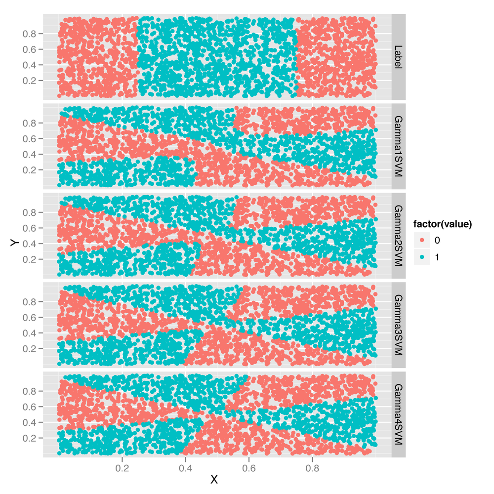
As you can see from looking at Figure 12-6, the rather complicated decision
boundary chosen by the sigmoid kernel warps around as we change the
value of gamma. To really get a better intuition for what’s
happening, we recommend that you experiment with many more values of
gamma than the four we’ve just shown you.
That ends our introduction to the SVM. We think it’s a valuable algorithm to have in your toolkit, but it’s time to stop building up your toolkit and instead start focusing on thinking critically about which tool is best for any given job. To do that, we’ll explore multiple models simultaneously on a single data set.
Since we know how to use to SVMs, logistic regression, and kNN, let’s compare their performance on the SpamAssassin data set we worked with in Chapters 3 and 4. Experimenting with multiple algorithms is a good habit to develop when working with real-world data because often you won’t be able to know in advance which algorithm will work best with your data set. Also, one of the major skills that separates the most experienced people in machine learning from those just starting to use it is the ability to know from the structure of a problem when a certain algorithm won’t work well. The best way to build up this intuition is to apply all of the standard algorithms to every problem you come across until you have a sense of when they’ll fail.
The first step is simply to load our data and preprocess it
appropriately. Because this was done in detail before, we’re going to skip
several steps and simply load a document-term matrix from disk using the
load function in R, which reads in a binary format that can
be used to write R objects to disk for long-term storage. Then we’ll do a training set/test set split and discard the
raw data set using the rm function, which allows us to
delete an object from memory:
load('data/dtm.RData')

set.seed(1)

training.indices <- sort(sample(1:nrow(dtm), round(0.5 * nrow(dtm))))
test.indices <- which(! 1:nrow(dtm) %in% training.indices)
train.x <- dtm[training.indices, 3:ncol(dtm)]
train.y <- dtm[training.indices, 1]
test.x <- dtm[test.indices, 3:ncol(dtm)]
test.y <- dtm[test.indices, 1]

rm(dtm)
Now that we have a data set in memory, we can immediately
move forward and fit a regularized logistic regression using
glmnet:
library('glmnet')
regularized.logit.fit <- glmnet(train.x, train.y, family = c('binomial'))
Of course, that still leaves us with a great deal of flexibility,
so we’d like to compare various settings for the lambda hyperparameter to see which gives us
the best performance. To push through this example quickly, we’ll cheat
a bit and test the hyperparameter settings on the test set rather than
do repeated splits of the training data. If you’re rigorously testing
models, you shouldn’t make this sort of simplification, but we’ll leave
the clean tuning of lambda as an
exercise for you to do on your own. For now, we’ll just try all of the
values that glmnet proposed and see which performs best on
the test set:
lambdas <- regularized.logit.fit$lambda
performance <- data.frame()

for (lambda in lambdas)
{
  predictions <- predict(regularized.logit.fit, test.x, s = lambda)
  predictions <- as.numeric(predictions > 0)
  mse <- mean(predictions != test.y)

  performance <- rbind(performance, data.frame(Lambda = lambda, MSE = mse))
}

ggplot(performance, aes(x = Lambda, y = MSE)) +
  geom_point() +
  scale_x_log10()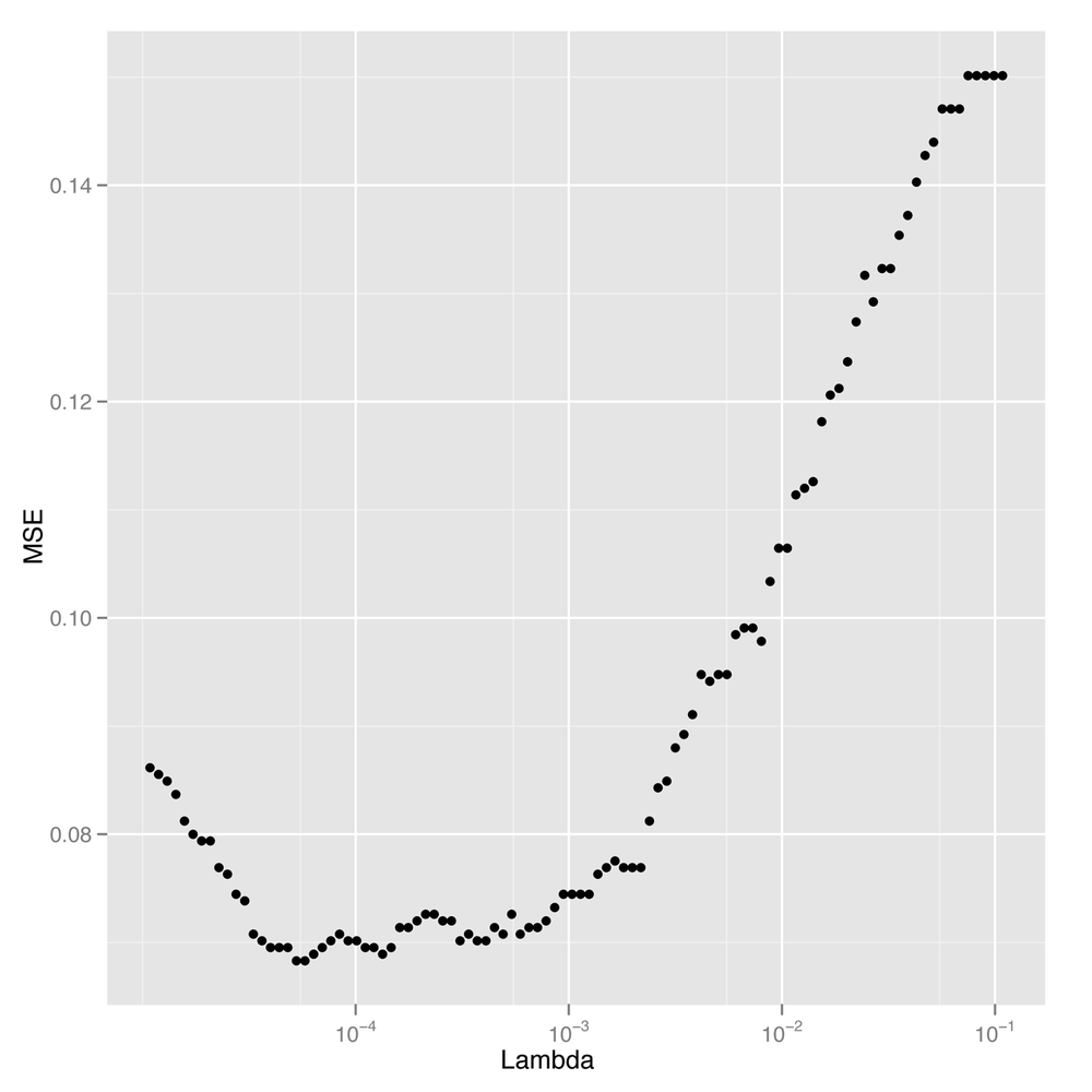
Looking at Figure 12-7,
we see a pretty clear region of values for lambda that gives the lowest possible error
rate. To find the best value for our final analysis, we can then use
simple indexing and the min function:
best.lambda <- with(performance, max(Lambda[which(MSE == min(MSE))]))
In this case, there are actually two different values of
lambda that give identical
performance, so we extract the larger of the two using the
max function. We choose the larger value because it is the
one with greater regularization applied. We can then calculate the MSE
for our logistic model using this best value for
lambda:
mse <- with(subset(performance, Lambda == best.lambda), MSE)
mse
#[1] 0.06830769
We can see that using regularized logistic regression, which requires only a trivial amount of hyperparameter tuning to implement, misclassifies only 6% of all emails in our test set. But we’d like to see how other methods do with similar amounts of work so that we can decide whether we should be using logistic regression, SVMs, or kNN.
For that reason, let’s start by fitting a linear kernel SVM to see how it compares with logistic regression:
library('e1071')
linear.svm.fit <- svm(train.x, train.y, kernel = 'linear')
Fitting the linear kernel SVM is a little bit slow with this large data set. For that reason, we’re going to be somewhat unfair to the SVM and simply use the default settings for the hyperparameters. As was the case with picking the ideal hyperparameter for logistic regression by assessing performance on our test set, this use of default hyperparameter values isn’t ideal, but it’s also a regular occurrence in the machine learning literature. When you compare models, you need to keep in mind that one of the things you see in your results is simply a measure of how hard you’ve worked to make each model fit the data. If you spend more time tuning one model than another, the differences in their performance can be partly attributable not to their differing structure, but to the different levels of effort you invested in them.
Knowing that, we’ll blindly forge ahead and assess the linear kernel SVM’s performance on our test data:
predictions <- predict(linear.svm.fit, test.x)
predictions <- as.numeric(predictions > 0)
mse <- mean(predictions != test.y)
mse
#0.128
We can see that we get a 12% error rate, which is double that of
the logistic regression model. To get a better sense of the real limits
of the linear kernel SVM, you should experiment with manipulating the
cost hyperparameter to find its ideal value before
estimating the error rate for the linear kernel SVM.
But for now we’ll just stick with the results we already have for the linear kernel SVM and move on to a radial kernel SVM to see how much the kernel changes the results we get in this practical problem that we can’t visualize in the same way we could visualize the toy problem at the start of this chapter:
radial.svm.fit <- svm(train.x, train.y, kernel = 'radial')

predictions <- predict(radial.svm.fit, test.x)
predictions <- as.numeric(predictions > 0)
mse <- mean(predictions != test.y)
mse
#[1] 0.1421538
Somewhat surprisingly, the radial kernel does a little worse on this data set than the linear kernel, which is the opposite of what we saw from our example of nonlinear data. And that’s an example of a broader lesson you’ll absorb with more experience working with data: the ideal model for your problem depends on the structure of your data. In this case, the inferior performance of the radial kernel SVM suggests that the ideal decision boundary for this problem might really be linear. That’s also supported by the fact that we’ve already seen that logistic regression is beating both the linear and the radial kernel SVMs. These sorts of observations are the most interesting ones we can make while comparing algorithms on a fixed data set because we learn something about the true structure of the data from the misfit of our models.
But before we stop fitting models and decide to stick with logistic regression, let’s try the method that works best with nonlinear data: kNN. Here we fit kNN using 50 neighbors for each prediction:
library('class')
knn.fit <- knn(train.x, test.x, train.y, k = 50)

predictions <- as.numeric(as.character(knn.fit))
mse <- mean(predictions != test.y)
mse
#[1] 0.1396923
As we can see, we get a 14% error from kNN, which is further
evidence that linear models are better for classifying spam than
nonlinear models. And because kNN doesn’t take so long to fit on this
data set, we’ll also try several values for k to see which
performs best:
performance <- data.frame()

for (k in seq(5, 50, by = 5))
{
  knn.fit <- knn(train.x, test.x, train.y, k = k)

  predictions <- as.numeric(as.character(knn.fit))
  mse <- mean(predictions != test.y)

  performance <- rbind(performance, data.frame(K = k, MSE = mse))
}

best.k <- with(performance, K[which(MSE == min(MSE))])
best.mse <- with(subset(performance, K == best.k), MSE)
best.mse
#[1] 0.09169231
With tuning, we see that we can get a 9% error rate from kNN. This is halfway between the performance we’ve seen for SVMs and logistic regression, as you can confirm by looking at Table 12-1, which collates the error rates we obtained with each of the four algorithms we’ve used on this spam data set.
Table 12-1. Model comparison results
| Model | MSE |
|---|---|
| Regularized logistic regression | 0.06830769 |
| Linear kernel SVM | 0.128 |
| Radial kernel SVM | 0.1421538 |
| kNN | 0.09169231 |
In the end, it seems that the best approach for this problem is to use logistic regression with a tuned hyperparameter for regularization. And that’s actually a reasonable conclusion because industrial-strength spam filters have all switched over to logistic regression and left the Naive Bayes approach we described in Chapter 3 behind. For reasons that aren’t entirely clear to us, logistic regression simply works better for this sort of problem.
What broader lessons should you take away from this example? We hope you’ll walk away with several lessons in mind: (1) you should always try multiple algorithms on any practical data set, especially because they’re so easy to experiment with in R; (2) the types of algorithms that work best are problem-specific; and (3) the quality of the results you get from a model are influenced by the structure of the data and also by the amount of work you’re willing to put into setting hyperparameters, so don’t shirk the hyperparameter tuning step if you want to get strong results.
To hammer those lessons home, we encourage you to go back through the four models we’ve fit in this chapter and set the hyperparameters systematically using repeated splits of the training data. After that, we encourage you to try the polynomial and sigmoid kernels that we neglected while working with the spam data. If you do both of these things, you’ll get a lot of experience with the nuts and bolts of fitting complicated models to real-world data, and you’ll learn to appreciate how differently the models we’ve shown you in this book can perform on a fixed data set.
On that note, we’ve come to the end of our final chapter and the book as a whole. We hope you’ve discovered the beauty of machine learning and gained an appreciation for the broad ideas that come up again and again when trying to build predictive models of data. We hope you’ll go on to study machine learning from the classic mathematical textbooks such as Hastie et al. HTF09 or Bishop Bis06, which cover the material we’ve described in a practical fashion from a theoretical bent. The best machine learning practitioners are those with both practical and theoretical experience, so we encourage you to go out and develop both.
Along the way, have fun hacking data. You have a lot of powerful tools, so go apply them to questions you’re interested in!