Table of Contents for
Machine Learning for Hackers
 Machine Learning for Hackers
Published by
O'Reilly Media, Inc., 2012
Machine Learning for Hackers
Published by
O'Reilly Media, Inc., 2012
- Cover
- O'Reilly Strata Conference
- Machine Learning for Hackers
- Preface
- 1. Using R
- 2. Data Exploration
- 3. Classification: Spam Filtering
- 4. Ranking: Priority Inbox
- 5. Regression: Predicting Page Views
- 6. Regularization: Text Regression
- 7. Optimization: Breaking Codes
- 8. PCA: Building a Market Index
- 9. MDS: Visually Exploring US Senator Similarity
- 10. kNN: Recommendation Systems
- 11. Analyzing Social Graphs
- 12. Model Comparison
- Works Cited
- Index
- About the Authors
- Colophon
- Copyright
So far we’ve treated most of the algorithms in this book as partial black boxes, in that we’ve focused on understanding the inputs you’re expected to use and the outputs you’ll get. Essentially, we’ve treated machine learning algorithms as a library of functions for performing prediction tasks.
In this chapter, we’re going to examine some of the techniques that are used to implement the most basic machine learning algorithms. As a starting point, we’re going to put together a function for fitting simple linear regression models with only one predictor. That example will allow us to motivate the idea of viewing the act of fitting a model to data as an optimization problem. An optimization problem is one in which we have a machine with some knobs that we can turn to change the machine’s settings and a way to measure how well the machine is performing with the current settings. We want to find the best possible settings, which will be those that maximize some simple measure of how well the machine is performing. That point will be called the optimum. Reaching it will be called optimization.
Once we have a basic understanding of how optimization works, we’ll embark on our major task: building a very simple code-breaking system that treats deciphering an encrypted text as an optimization problem.
Because we’re going to build our own linear regression function, let’s go back to our standard example data set: people’s heights and weights. As we’ve already done, we’re going to assume that we can predict weights by computing a function of their heights. Specifically, we’ll assume that a linear function works, which looks like this in R:
height.to.weight <- function(height, a, b)
{
  return(a + b * height)
}
In Chapter 5
we went through the details of computing the slope and
intercept of this line using the lm function. In this
example, the a parameter is the slope of the line and the
b parameter is the intercept, which tells us how much a
person whose height is zero should weigh.
With this function in hand, how can we decide which values of
a and b are best? This is where optimization
comes in: we want to first define a measure of how well our function
predicts weights from heights and then change the values of
a and b until we predict as well as we
possibly can.
How do we do this? Well, lm already does all of this
for us. It has a simple error function that it tries to optimize, and it
finds the best values for a and b using a very
specific algorithm that works only for ordinary linear
regression.
Let’s just run lm to see its preferred values for
a and b:
heights.weights <- read.csv('data/01_heights_weights_genders.csv')

coef(lm(Weight ~ Height, data = heights.weights))
#(Intercept)      Height
#-350.737192    7.717288
Why are these reasonable choices for a and
b? To answer that, we need to know what error function
lm is using. As we said briefly in Chapter 5, lm
is based on an error measure called “squared error,” which
works in the following way:
Fix values for
aandb.Given a value for height, make a guess at the associated weight.
Take the true weight, and subtract the predicted weight. Call this the error.
Square the error.
Sum the squared errors over all of your examples to get your sum of squared errors.
Note
For interpretation, we usually take the mean rather than the sum, and compute square roots. But for optimization, none of that is truly necessary, so we can save some small amount of computational time by just calculating the sum of squared errors.
The last two steps are closely related; if we weren’t summing the errors for each data point together, squaring wouldn’t be helpful. Squaring is essential precisely because summing all of the raw errors together would give us zero total error.
Note
Showing that this is always true isn’t hard, but requires the sort of algebra we’re trying to avoid in this book.
Let’s go through some code that implements this approach:
squared.error <- function(heights.weights, a, b)
{
  predictions <- with(heights.weights, height.to.weight(Height, a, b))
  errors <- with(heights.weights, Weight - predictions)
  return(sum(errors ^ 2))
}
Let’s evaluate squared.error at some specific values
of a and b to get a sense of how this works
(the results are in Table 7-1):
for (a in seq(-1, 1, by = 1))
{
  for (b in seq(-1, 1, by = 1))
  {
    print(squared.error(heights.weights, a, b))
  }
}
Table 7-1. Squared error over a grid
| a | b | Squared error |
|---|---|---|
| -1 | -1 | 536271759 |
| -1 | 0 | 274177183 |
| -1 | 1 | 100471706 |
| 0 | -1 | 531705601 |
| 0 | 0 | 270938376 |
| 0 | 1 | 98560250 |
| 1 | -1 | 527159442 |
| 1 | 0 | 267719569 |
| 1 | 1 | 96668794 |
As you can see, some values of a and b
give much lower values for squared.error than others. That means we really want to find the best values
for a and b now that we have a meaningful
error function that tells us something about our ability to make
predictions. That’s the first part of our optimization problem: set up a
metric that we can then try to minimize or maximize. That metric is usually called our objective
function. The problem of optimization then becomes the
problem of finding the best values for a and b
to make that objective function as small or as big as possible.
One obvious approach is called grid search: compute a table
like the one we just showed you for a large enough range of values of
a and b, and then pick the row with the lowest
value of squared.error. This approach will always give you
the best value in the grid you’ve searched, so it’s not an unreasonable
approach. But there are some serious problems with it:
How close should the values you use to define the grid be to each other? Should
abe the values 0, 1, 2, 3? Or shouldabe the values 0, 0.001, 0.002, 0.003? In other words, what is the right resolution at which we should perform our search? Answering this question requires that you evaluate both grids and see which is more informative, an evaluation that is computationally costly and effectively introduces another a second optimization problem in which you’re optimizing the size of the grid you use. Down that road lies infinite loop madness.If you want to evaluate this grid at 10 points per parameter for 2 parameters, you need to build a table with 100 entries. But if you want this evaluate this grid at 10 points per parameter for 100 parameters, you need to build a table with 10^100 entries. This problem of exponential growth is so widespread in machine learning that it’s called the Curse of Dimensionality.
Because we want to be able to use linear regression with hundreds
or even thousands of inputs, grid search is out for good as an
optimization algorithm. So what can we do? Thankfully for us, computer
scientists and mathematicians have been thinking about the problem of
optimization for a long time and have built a large set of off-the-shelf
optimization algorithms that you can use. In R, you should usually make a first pass at an
optimization problem using the optim function, which
provides a black box that implements many of the most popular
optimization algorithms.
To show you how optim works, we’re going to use it to
fit our linear regression model. We hope that it produces values for
a and b that are similar to those produced by
lm:
optim(c(0, 0),
      function (x)
      {
        squared.error(heights.weights, x[1], x[2])
      })
#$par
#[1] -350.786736    7.718158
#
#$value
#[1] 1492936
#
#$counts
#function gradient
#     111       NA
#
#$convergence
#[1] 0
#
#$message
#NULL
As the example shows, optim takes a few different
arguments. First, you have to pass a numeric vector of starting points
for the parameters you’re trying to optimize; in this case, we say that
a and b should default to the vector
c(0, 0). After that, you have to pass a function to
optim that expects to receive a vector, which we’ve called
x, that contains all of the parameters you want to
optimize. Because we usually prefer writing functions with multiple
named parameters, we like wrapping our error function in an anonymous
function that takes only the argument x, which we then
partition out to our primary error function. In this example, you can
see how we’ve wrapped squared.error.
Running this call to optim gives us values for
a and b, respectively, as the values of
par. And these values are very close to those produced by
lm, which suggests that optim is working.[12] In practice, lm uses an algorithm
that’s much more specific to linear regression than our call to
optim, which makes the results more precise than those
produced by optim. If you’re going to work through your own
problems, though, optim is much better to work with because
it can be used with models other than linear regression.
The other outputs we get from optim are sometimes
less interesting. The first we’ve shown is value, which
tells us the value of the squared error evaluated at the parameters that
optim claims are best. After that, the counts
value tells us how many times optim evaluated the main
function (here called function) and the gradient (here called gradient), which is an
optional argument that can be passed if you know enough calculus to
compute the gradient of the main function.
Note
If the term “gradient” doesn’t mean anything to you, don’t
worry. We dislike calculating gradients by hand, and so we usually
let optim do its magic without specifying any value for
the optional gradient argument. Things have worked out pretty well
so far for us, though your mileage may vary.
The next value is convergence, which tells us
whether or not optim found a set of parameters it’s
confident are the best possible. If everything went well, you’ll see a
0. Check the documentation for optim for an interpretation
of the different error codes you can get when your result isn’t 0.
Finally, the message value tells us whether anything
happened that we need to know about.
In general, optim is based on a lot of clever ideas
from calculus that help us perform optimization. Because it’s quite
mathematically complex, we won’t get into the inner workings of
optim at all. But the general spirit of what
optim is doing is very simple to express graphically.
Imagine that you only wanted to find the best value of a
after you decided that b had to be 0. You could calculate
the squared error when you vary only a using the following
code:
a.error <- function(a)
{
return(squared.error(heights.weights, a, 0))
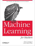
}To get a sense of where the best value of a is,
you can graph the squared error as a function of a using
the curve function in R, which will evaluate a function or
expression at a set of many values of a variable x and then
plot the output of that function or the value of the expression.
In the following example, we’ve evaluated
a.error at many values of x, and because of a
quirk in R’s evaluation of expressions, we’ve had to use
sapply to get things to work.
curve(sapply(x, function (a) {a.error(a)}), from = -1000, to = 1000)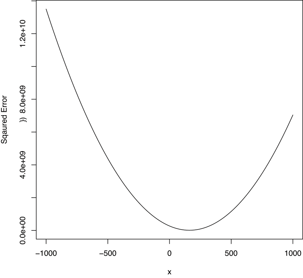
Looking at Figure 7-1, there
seems to be a single value for a that’s best, and every
value that moves further away from that value for a is
worse. When this happens, we say that there’s a global optimum. In cases like that,
optim can use the shape of the squared error function to
figure out in which direction to head after evaluating the error
function at a single value of a; using this local
information to learn something about the global structure of your
problem lets optim hit the optimum very quickly.
To get a better sense of the full regression problem, we also need
to look at how the error function responds when we change
b:
b.error <- function(b)
{
  return(squared.error(heights.weights, 0, b))
}

curve(sapply(x, function (b) {b.error(b)}), from = -1000, to = 1000)
Looking at Figure 7-2, the
error function looks like it also has a global optimum for
b. Taken together with evidence that there’s a global
optimum for a, this suggests that it should be possible for
optim to find a single best value for both a
and b that minimizes our error function.
More generally, we can say that optim works because
it can search for the troughs of these graphs in all of the parameters
at once by using calculus. It works faster than grid search because it
can use information about the point it’s currently considering to infer
something about nearby points. That lets it decide which direction it
should move in to improve its performance. This adaptive behavior makes
it much more efficient than grid search.
Now that we know a little bit about how to use
optim, we can start to use optimization algorithms to
implement our own version of ridge regression. Ridge regression is a specific kind of regression that
incorporates regularization, which we discussed in Chapter 6. The only difference between
ordinary least squares regression and ridge regression is the error
function: ridge regression considers the size of the regression
coefficients to be part of the error term, which encourages the
coefficients to be small. In this example, this pushes the slope and
intercept toward zero.
Other than changing our error function, the only added
complexity to running ridge regression is that we now have to include an
extra parameter, lambda, that adjudicates between the
importance of minimizing the squared error of our predictions and
minimizing the values of a and b so that we
don’t overfit our data. The extra parameter for this regularized
algorithm is called a hyperparameter and was discussed in some detail in
Chapter 6. Once we’ve selected a
value of lambda, we can write the ridge error function as
follows:
ridge.error <- function(heights.weights, a, b, lambda)
{
  predictions <- with(heights.weights, height.to.weight(Height, a, b))
  errors <- with(heights.weights, Weight - predictions)
  return(sum(errors ^ 2) + lambda * (a ^ 2 + b ^ 2))
}
As we discussed in Chapter 6, we can select a value of
lambda using cross-validation. For the rest of this
chapter, we’re simply going to assume that you’ve already done this and
that the proper value of lambda is 1.
With the ridge error function defined in R, a new call to
optim solves the ridge regression problem as easily as the
original ordinary least squares problem was solved:
lambda <- 1

optim(c(0, 0),
      function (x)
      {
        ridge.error(heights.weights, x[1], x[2], lambda)
      })
#$par
#[1] -340.434108    7.562524
#
#$value
#[1] 1612443
#
#$counts
#function gradient
#     115       NA
#
#$convergence
#[1] 0
#
#$message
#NULL
Looking at the output of optim, we can see that we’ve
produced a slightly smaller intercept and slope for our line than we had
when using lm, which gave an intercept of -350
and a slope of 7.7. In this toy example that’s not really
helpful, but in the large-scale regressions we ran in Chapter 6, including a penalty for
large coefficients was essential to getting meaningful results out of
our algorithm.
In addition to looking at the fitted coefficients, we can
also repeat the calls we were making to the curve function
to see why optim should be able work with ridge regression
in the same way that it worked for ordinary linear regression. The
results are shown in Figures 7-3 and 7-4.
a.ridge.error <- function(a, lambda)
{
  return(ridge.error(heights.weights, a, 0, lambda))
}

curve(sapply(x, function (a) {a.ridge.error(a, lambda)}), from = -1000, to = 1000)
b.ridge.error <- function(b, lambda)
{
return(ridge.error(heights.weights, 0, b, lambda))
}
curve(sapply(x, function (b) {b.ridge.error(b, lambda)}), from = -1000, to = 1000)Hopefully this example convinces you that you can get a lot done
in machine learning just by understanding how to use functions such as
optim to minimize some measure of prediction error. We
recommend working through a few examples on your own and then playing
around with different error functions that you’ve invented yourself.
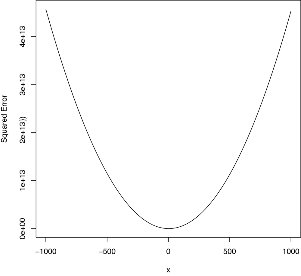
This is particularly helpful when you try an error function like the
absolute error function shown here:
absolute.error <- function
(heights.weights, a, b)
{
  predictions <- with(heights.weights, height.to.weight(Height, a, b))
  errors <- with(heights.weights, Weight - predictions)
  return(sum(abs(errors)))
}
For technical reasons related to calculus, this error term won’t
play nice with optim. Fully explaining why things break is
a little hard without calculus, but it’s actually possible to
communicate the big idea visually. We just repeat the calls to
curve that we’ve been making:
a.absolute.error <- function(a)
{
  return(absolute.error(heights.weights, a, 0))
}

curve(sapply(x, function (a) {a.absolute.error(a)}), from = -1000, to = 1000)

As you can see in Figure 7-5, the absolute error curve is
much sharper than the squared error curve or the ridge error curve.
Because the shape is so sharp, optim doesn’t get as much
information about the direction in which it should go from a single
point and won’t necessarily reach the global optimum, even though we can
clearly see that one exists from simple visual inspection.
Because some types of error metrics break otherwise powerful
algorithms, part of the art of doing machine learning well is learning
when simple tools like optim will work and learning when
you’ll need something more powerful. There are algorithms that work for
absolute error optimization, but they’re beyond the scope of this book.
If you’re interested in learning more about this, find your local math
guru and get him to talk to you about convex optimization.
Moving beyond regression models, almost every algorithm in
machine learning can be viewed as an optimization problem in which we
try to minimize some measure of prediction error. But sometimes our
parameters aren’t simple numbers, and so evaluating your error function
at a single point doesn’t give you enough information about nearby
points to use optim. For these problems, we could use grid
search, but there are other approaches that work better than grid
search. We’ll focus on one approach that’s fairly intuitive and very
powerful. The big idea behind this new approach, which we’ll call
stochastic optimization, is to move through the range of possible
parameters slightly randomly, but making sure to head in directions
where your error function tends to go down rather than up. This approach
is related to a lot of popular optimization algorithms that you may have
heard of, including simulated annealing, genetic algorithms, and Markov
chain Monte Carlo (MCMC). The specific algorithm we’ll use is called the Metropolis
method; versions of the Metropolis method power a lot of modern machine
learning algorithms.
To illustrate the Metropolis method, we’ll work through this
chapter’s case study: breaking secret codes. The algorithm we’re going
to define isn’t a very efficient decryption system and would never be
seriously used for production systems, but it’s a very clear example of
how to use the Metropolis method. Importantly, it’s also an example
where most out-of-the-box optimization algorithms such as
optim could never
work.
So let’s state our problem: given a string of letters that you know are encrypted using a substitution cipher, how do we decide on a decryption rule that gives us the original text? If you’re not familiar with substitution ciphers, they’re the simplest possible encryption system, in which you replace every letter in the unencrypted message with a fixed letter in the encrypted message. ROT13[13] is probably the most famous example, though the Caesar cipher might also be known to you. The Caesar cipher is one very simple substitution cipher in which you replace every letter with its neighbor in the alphabet: “a” becomes “b,” “b” becomes “c,” and “c” becomes “d.” (If you’re wondering about the edge case here: “z” becomes “a.”)
To make sure it’s clear how to work with ciphers in R, let’s create the Caesar cipher for now so that we can see how to implement it in R:
english.letters <- c('a', 'b', 'c', 'd', 'e', 'f', 'g', 'h', 'i', 'j', 'k',
                     'l', 'm', 'n', 'o', 'p', 'q', 'r', 's', 't', 'u', 'v',
                     'w', 'x', 'y', 'z')

caesar.cipher <- list()
inverse.caesar.cipher <- list()

for (index in 1:length(english.letters))
{
  caesar.cipher[[english.letters[index]]] <- english.letters[index %% 26 + 1]
  inverse.caesar.cipher[[english.letters[index %% 26 + 1]]] <- english.letters[index]
}

print(caesar.cipher)
Now that we have the cipher implemented, let’s build some functions so that we can translate a string using a cipher:
apply.cipher.to.string <- function(string, cipher)
{
  output <- ''

  for (i in 1:nchar(string))
  {
    output <- paste(output, cipher[[substr(string, i, i)]], sep = '')
  }

  return(output)
}

apply.cipher.to.text <- function(text, cipher)
{
  output <- c()

  for (string in text)
  {
    output <- c(output, apply.cipher.to.string(string, cipher))
  }

  return(output)
}

apply.cipher.to.text(c('sample', 'text'), caesar.cipher)
Now we have some basic tools for working with ciphers, so let’s start thinking about the problem of breaking the codes we might come across. Just as we did with linear regression, we’ll solve the problem of breaking substitution ciphers in several parts:
Define a measure of the quality of a proposed decryption rule.
Define an algorithm for proposing new potential decryption rules that randomly modifies versions of our current best rule.
Define an algorithm for moving progressively toward better decryption rules.
To start thinking about how to measure the quality of decryption rule, let’s suppose that you were given a piece of text that you knew had been encrypted using a substitution cipher. For example, if Julius Caesar had sent an encrypted message to you, it might look like this: “wfoj wjej wjdj.” After inverting the Caesar cipher, this text will turn out to be the famous phrase “veni vidi vici.”
Now imagine that you only had a piece of encrypted text and a guarantee that the original message was in standard English. How would you go about decoding it?
The approach we’re going to take here to solving that problem is to say that a rule is good if it turns the encrypted message into normal English. Given a proposed decryption rule, you’ll run the rule on our encrypted text and see whether the output is realistic English. For example, imagine that we had two proposed decryption rules, A and B, whose results are the following:
decrypt(T, A) = xgpk xkfk xkek
decrypt(T, B) = veni vidi vici
After seeing the outputs from the two proposed rules, you think it’s pretty clear that rule B is better than rule A. How are we making this intuitive decision? We can tell that B is better than A because the text from rule B looks like real language rather than nonsense, whereas rule A’s text looks completely nonsensical. To transform that human intuition into something automatic that we can program a computer to do, we’ll use a lexical database that provides the probability for any word we see. Real language will then be equivalent to text built out of words that have high probability, whereas fake language will be equivalent to text with words that have low probability. The only complexity with this approach is dealing with words that don’t exist at all. Because their probability is zero and we’re going to estimate the probability of a piece of text as a whole by multiplying the probability of the individual words together, we’ll need to replace zero with something really small, like our machine’s smallest distinguishable floating-point difference, which we’ll call epsilon, to use our algorithm. Once we’ve handled that edge case, we can use a lexical database to rank the quality of two pieces of translated text by finding the probability of each word and then multiplying these probabilities together to find an estimate of the probability of the text as a whole.
Using a lexical database to calculate the probability of the decrypted text will give us our error metric for evaluating a proposed decryption rule. Now that we have an error function, our code-breaking problem has turned entirely into a optimization problem, so we just need to find decryption rules that produce text with high probability.
Unfortunately, the problem of finding the rule with the highest
text probability isn’t close to being the sort of problem where
optim would work. Decryption rules can’t be graphed and
don’t have the smoothness that optim needs when it’s trying
to figure how to head toward better rules. So we need a totally new
optimization algorithm for solving our decryption problem. That
algorithm is going to be the Metropolis method that we already mentioned
at the start of this section. The Metropolis algorithm turns out to work
relatively well for our problem, though it’s very, very slow for any
reasonable length of text.[14]
The basic idea for the Metropolis method is that we’ll start with an arbitrary decryption rule and then iteratively improve it many times so that it becomes a rule that could feasibly be the right one. This may seem like magic at first, but it often works in practice, as you should convince yourself by experimentation. And once we have a potential decryption rule in hand, we can use our human intuition based on semantic coherence and grammar to decide whether we’ve correctly decrypted the text.
To generate a good rule, we start with a completely arbitrary rule and then repeat a single operation that improves our rule a large number of times—say, 50,000 times. Because each step tends to head in the direction of better rules, repeating this operation over and over again will get us somewhere reasonable in the end, though there’s no guarantee that we won’t need 50,000,000 steps rather than 50,000 to get where we’d like to be. That’s the reason this algorithm won’t work well for a serious code-breaking system: you have no guarantee that the algorithm will give you a solution in a reasonable amount of time, and it’s very hard to tell if you’re even moving in the right direction while you’re waiting. This case study is just a toy example that shows off how to use optimization algorithms to solve complex problems that might otherwise seem impossible to solve.
Let’s be specific about how we’re going to propose a new decryption rule. We’ll do it by randomly disturbing the current rule in just one place. That is, we’ll disturb our current rule by changing the rule’s effect on a single letter of the input alphabet. If “a” currently translates to “b” under our rule, we’ll propose a modification that has “a” translate to “q.” Because of the way substitution ciphers works, this will actually require another modification to the part of the rule that originally sent another letter—for example, “c”—to “q.” To keep our cipher working, “c” now has to translate to “b.” So our algorithm for proposing new rules boils down to making two swaps in our existing rule, one randomly selected and another one forced by the definition of a substitution cipher.
If we were naive, we would accept this new proposed rule only if it increased the probability of our decrypted text. That’s called greedy optimization. Unfortunately, greedy optimization in this case will tend to leave us stuck at bad rules, so we’ll use the following nongreedy rule to decide between our original rule A and our new rule B instead:
If the probability of the text decrypted with rule B is greater than the probability of the text decrypted with rule A, then we replace A with B.
If the probability of the text decrypted with rule B is less than the probability of the text decrypted with rule A, we’ll still replace A with B sometimes, just not every time. To be specific, if the probability of the text decrypted with rule B is
probability(T, B)and the probability of the text decrypted with rule A isprobability(T, A), we’ll switch over to rule Bprobability(T, B) / probability(T, A) percentof the time.Note
If this ratio seems to have come out of left field, don’t worry. For intuition’s sake, what really matters isn’t the specific ratio, but the fact that we accept rule B more than 0% of the time. That’s what helps us to avoid the traps that greedy optimization would have us fall into.
Before we can use the Metropolis method to sort through different ciphers, we need some tools for creating the perturbed ciphers we’ve just described. Here they are:
generate.random.cipher <- function()
{
  cipher <- list()

  inputs <- english.letters
  outputs <- english.letters[sample(1:length(english.letters),
  length(english.letters))]

  for (index in 1:length(english.letters))
  {
    cipher[[inputs[index]]] <- outputs[index]
  }

  return(cipher)
}

modify.cipher <- function(cipher, input, output)
{
  new.cipher <- cipher
  new.cipher[[input]] <- output
  old.output <- cipher[[input]]
  collateral.input <- names(which(sapply(names(cipher),
                      function (key) {cipher[[key]]}) == output))
  new.cipher[[collateral.input]] <- old.output
  return(new.cipher)
}

propose.modified.cipher <- function(cipher)
{
  input <- sample(names(cipher), 1)
  output <- sample(english.letters, 1)
  return(modify.cipher(cipher, input, output))
}
Combining this tool for proposing new rules and the rule-swapping
procedure we specified softens the greediness of our optimization
approach without making us waste too much time on obviously bad rules
that have much lower probability than our current rule. To do this
softening algorithmically, we just compute probability(T, B) /
probability(T , A) and compare it with a random number between 0
and 1. If the resulting random number is higher than
probability(T, B) / probability(T , A), we replace our
current rule. If not, we stick with our current rule.
In order to compute the probabilities that we keep mentioning, we’ve created a lexical database that tells you how often each of the words in /usr/share/dic/words occurs in text on Wikipedia. To load that into R, you would do the following:
load('data/lexical_database.Rdata')You can get a feel for the database by querying some simple words and seeing their frequencies in our sample text (see Table 7-2):
lexical.database[['a']]
lexical.database[['the']]
lexical.database[['he']]
lexical.database[['she']]
lexical.database[['data']]
Table 7-2. Lexical database
| Word | Probability |
|---|---|
| a | 0.01617576 |
| the | 0.05278924 |
| he | 0.003205034 |
| she | 0.0007412179 |
| data | 0.0002168354 |
Now that we have our lexical database, we need some methods to
calculate the probability of text. First, we’ll write a function to wrap
pulling the probability from the database. Writing a function makes it
easier to handle fake words that need to be assigned the lowest possible probability,
which is going to be your machine’s floating-point epsilon. To get access to
that value in R, you can use the variable
.Machine$double.eps.
one.gram.probability <- function(one.gram, lexical.database = list())
{
  lexical.probability <- lexical.database[[one.gram]]

  if (is.null(lexical.probability) || is.na(lexical.probability))
  {
    return(.Machine$double.eps)
  }
  else
  {
    return(lexical.probability)
  }
}
Now that we have this method for finding the probability of isolated words, we create a method for calculating the probability of a piece of text by pulling the text apart into separate words, calculating probabilities in isolation, and putting them back together again by multiplying them together. Unfortunately, it turns out that using raw probabilities is numerically unstable because of the finite precision arithmetic that floating-point numbers provide when you do multiplication. For that reason, we actually compute the log probability of the text, which is just the sum of the log probabilities of each word in the text. That value turns out to be not to be numerically unstable.
log.probability.of.text <- function(text, cipher, lexical.database = list())
{
  log.probability <- 0.0

  for (string in text)
  {
    decrypted.string <- apply.cipher.to.string(string, cipher)
    log.probability <- log.probability +
    log(one.gram.probability(decrypted.string, lexical.database))
  }

  return(log.probability)
}
Now that we have all the administrative components we need, we can write a single step of the Metropolis method as follows:
metropolis.step <- function(text, cipher, lexical.database = list())
{
  proposed.cipher <- propose.modified.cipher(cipher)

  lp1 <- log.probability.of.text(text, cipher, lexical.database)
  lp2 <- log.probability.of.text(text, proposed.cipher, lexical.database)

  if (lp2 > lp1)
  {
    return(proposed.cipher)
  }
  else
  {
    a <- exp(lp2 - lp1)
    x <- runif(1)
    if (x < a)
    {
      return(proposed.cipher)
    }
    else
    {
      return(cipher)
    }
  }
}
And now that we have the individual steps of our optimization algorithm working, let’s put them together in a single example program that shows how they work. First, we’ll set up some raw text as a character vector in R:
decrypted.text <- c('here', 'is', 'some', 'sample', 'text')Then we’ll encrypt this text using the Caesar cipher:
encrypted.text <- apply.cipher.to.text(decrypted.text, caesar.cipher)
From there, we’ll create a random decryption cipher, run 50,000
Metropolis steps, and store the results in a data.frame
called results. For each step, we’ll keep a record of the
log probability of the decrypted text, the current decryption of the
sample text, and a dummy variable indicating whether we’ve correctly
decrypted the input text.
Warning
Of course, if you were really trying to break a secret code, you wouldn’t be able to tell when you’d correctly decrypted the text, but it’s useful to keep a record of this for demo purposes.
set.seed(1)
cipher <- generate.random.cipher()

results <- data.frame()

number.of.iterations <- 50000

for (iteration in 1:number.of.iterations)
{
  log.probability <- log.probability.of.text(encrypted.text, cipher, lexical.database)
  current.decrypted.text <- paste(apply.cipher.to.text(encrypted.text, cipher),
                                  collapse = ' ')
  correct.text <- as.numeric(current.decrypted.text == paste(decrypted.text,
                                                             collapse = ' '))
  results <- rbind(results,
                   data.frame(Iteration = iteration,
                              LogProbability = log.probability,
                              CurrentDecryptedText = current.decrypted.text,
                              CorrectText = correct.text))
  cipher <- metropolis.step(encrypted.text, cipher, lexical.database)
}

write.table(results, file = 'data/results.csv', row.names = FALSE, sep = '\t')
It takes a while for this code to run, so while you’re waiting, let’s look at a sample of the results contained in Table 7-3.
Table 7-3. Progress of the Metropolis method
| Iteration | Log probability | Current decrypted text |
|---|---|---|
| 1 | -180.218266945586 | lsps bk kfvs kjvhys zsrz |
| 5000 | -67.6077693543898 | gene is same sfmpwe text |
| 10000 | -67.6077693543898 | gene is same spmzoe text |
| 15000 | -66.7799669880591 | gene is some scmhbe text |
| 20000 | -70.8114316132189 | dene as some scmire text |
| 25000 | -39.8590155606438 | gene as some simple text |
| 30000 | -39.8590155606438 | gene as some simple text |
| 35000 | -39.8590155606438 | gene as some simple text |
| 40000 | -35.784429416419 | were as some simple text |
| 45000 | -37.0128944882928 | were is some sample text |
| 50000 | -35.784429416419 | were as some simple text |
As you can see, we’re close to the correct decryption after the 45,000 step, but we’re not quite there. If you drill down into the results with greater detail, you’ll discover that we hit the correct text at row 45,609, but then we moved past the correct rule to a different rule. This is actually a problem with our objective function: it’s not really assessing whether the translation is English, but only whether the individual words are all normal English words. If changing the rule gives you a more probable word, you’ll tend to move in that direction, even if the result is grammatically broken or semantically incoherent. You could use more information about English, such as the probability of sequences of two words, to work around this. For now, we think it highlights the complexities of using optimization approaches with ad hoc objective functions: sometimes the solution you want isn’t the solution that your rule will decide is best. Humans need to be kept in the loop when you’re using optimization algorithms to solve your problems.
In truth, things are even more complicated than problems with our objective function not containing enough knowledge about how English works. First, the Metropolis method is always a random optimization method. Luckily we started off with a good seed value of 1, but a bad seed value could mean that it would take trillions of steps before we hit the right decryption rule. You can convince yourself of this by playing with the seed we’ve used and running only 1,000 iterations for each seed.
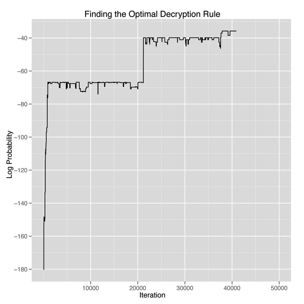
Second, the Metropolis method is always going to be willing to leave good translations. That’s what makes it a nongreedy algorithm, so you can often watch it abandon the solution you want it to find if you follow the trace of its progress long enough. In Figure 7-6, we show the log probability of the decrypted text at every step along the way. You can see how erratic the method’s movement is.
There are popular ways to deal with this random movement. One is to make the method progressively more greedy over time by accepting nongreedy proposed rules less often. That’s called simulated annealing, and it’s a very powerful approach to optimization that you can play with in our example simply by changing the way you accept new decryption rules.[15]
Another way to deal with this randomness is to embrace it and use it to produce a distribution of possible answers rather than a single right answer. In this problem that’s not very helpful, but in problems where the right answer is a number, it can be very helpful to produce of variety of possible answers.
In closing, we hope that you’ve gained some insight into how optimization works in general and how you can use it to solve complicated problems in machine learning. We’ll use some of those ideas again in later chapters, especially when talking about recommendation systems.
[12] Or at least that it’s doing the same wrong thing as
lm.
[13] ROT13 replaces every letter with the letter 13 positions further in the alphabet. “a” becomes “n,” “b’” becomes “o,” and so on.
[14] The slowness is considerably exacerbated by R’s slow text-processing tools, which are much less efficient than a language like Perl’s.
[15] In fact, there’s an argument to optim that will
force optim to use simulated annealing instead of its
standard optimization algorithm. In our example, we can’t use
optim’s implementation of simulated annealing because
it works only with numerical parameters and can’t handle the data
structure we’re using to represent ciphers.