Table of Contents for
Machine Learning for Hackers
 Machine Learning for Hackers
Published by
O'Reilly Media, Inc., 2012
Machine Learning for Hackers
Published by
O'Reilly Media, Inc., 2012
- Cover
- O'Reilly Strata Conference
- Machine Learning for Hackers
- Preface
- 1. Using R
- 2. Data Exploration
- 3. Classification: Spam Filtering
- 4. Ranking: Priority Inbox
- 5. Regression: Predicting Page Views
- 6. Regularization: Text Regression
- 7. Optimization: Breaking Codes
- 8. PCA: Building a Market Index
- 9. MDS: Visually Exploring US Senator Similarity
- 10. kNN: Recommendation Systems
- 11. Analyzing Social Graphs
- 12. Model Comparison
- Works Cited
- Index
- About the Authors
- Colophon
- Copyright
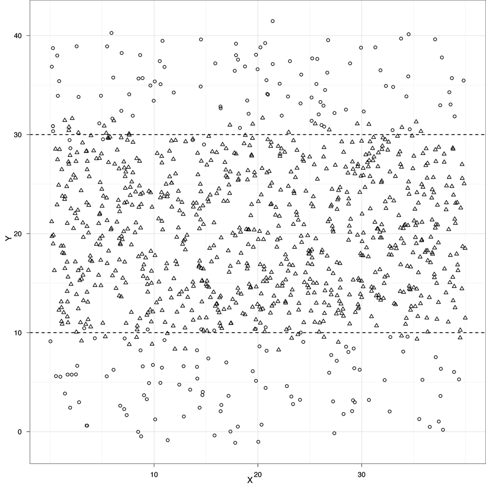
At the very end of Chapter 2, we quickly presented an example of classification. We used heights and weights to predict whether a person was a man or a woman. With our example graph, we were able to draw a line that split the data into two groups: one group where we would predict “male” and another group where we would predict “female.” This line was called a separating hyperplane, but from now on we’ll use the term “decision boundary,” because we’ll be working with data that can’t be classified properly using only straight lines. For example, imagine that your data looked like the data set shown in Example 3-1.
This plot might depict people who are at risk for a certain ailment and those who are not. Above and below the black horizontal lines we might predict that a person is at risk, but inside we would predict good health. These black lines are thus our decision boundary. Suppose that the blue dots represent healthy people and the red dots represent people who suffer from a disease. If that were the case, the two black lines would work quite well as a decision boundary for classifying people as either healthy or sick.
Producing general-purpose tools that let us handle problems where the decision boundary isn’t a single straight line has been one of the great achievements of machine learning. One approach in particular that we’ll focus on later is called the kernel trick, which has the remarkable property of allowing us to work with much more sophisticated decision boundaries at almost no additional computational cost.
But before we begin to understand how these decision boundaries are determined in practice, let’s review some of the big ideas in classification.
We’re going to assume that we have a set of labeled examples of the categories we want to learn how to identify. These examples consist of a label, which we’ll also call a class or type, and a series of measured variables that describe each example. We’ll call these measurements features or predictors. The height and weight columns we worked with earlier are examples of features that we could use to guess the “male” and “female” labels we were working with before.
Examples of classifications can be found anywhere you look for them:
Given the results of a mammogram, does a patient have breast cancer?
Do blood pressure measurements suggest that a patient has hypertension?
Does a political candidate’s platform suggest that she is a Republican candidate or a Democratic candidate?
Does a picture uploaded to a social network contain a face in it?
Was The Tempest written by William Shakespeare or Francis Bacon?
In this chapter, we’re going to focus on problems with text classification that are closely related to the tools you could use to answer the last question in our list. In our exercise, however, we’re going to build a system for deciding whether an email is spam or ham.
Our raw data comes from the SpamAssassin public corpus, available for free download at http://spamassassin.apache.org/publiccorpus/. Portions of this corpus are included in the code/data/ folder for this chapter and will be used throughout this chapter. At the unprocessed stage, the features are simply the contents of the raw email as plain text.
This raw text provides us with our first problem. We need to transform our raw text data into a set of features that describe qualitative concepts in a quantitative way. In our case, that will be a 0/1 coding strategy: spam or ham. For example, we may want to determine the following: “Does containing HTML tags make an email more likely to be spam?” To answer this, we will need a strategy for turning the text in our email into numbers. Fortunately, the general-purpose text-mining packages available in R will do much of this work for us.
For that reason, much of this chapter will focus on building up your intuition for the types of features that people have used in the past when working with text data. Feature generation is a major topic in current machine learning research and is still very far from being automated in a general-purpose way. At present, it’s best to think of the features being used as part of a vocabulary of machine learning that you become more familiar with as you perform more machine learning tasks.
Note
Just as learning the words of a new language builds up an intuition for what could realistically be a word, learning about the features people have used in the past builds up an intuition for what features could reasonably be helpful in the future.
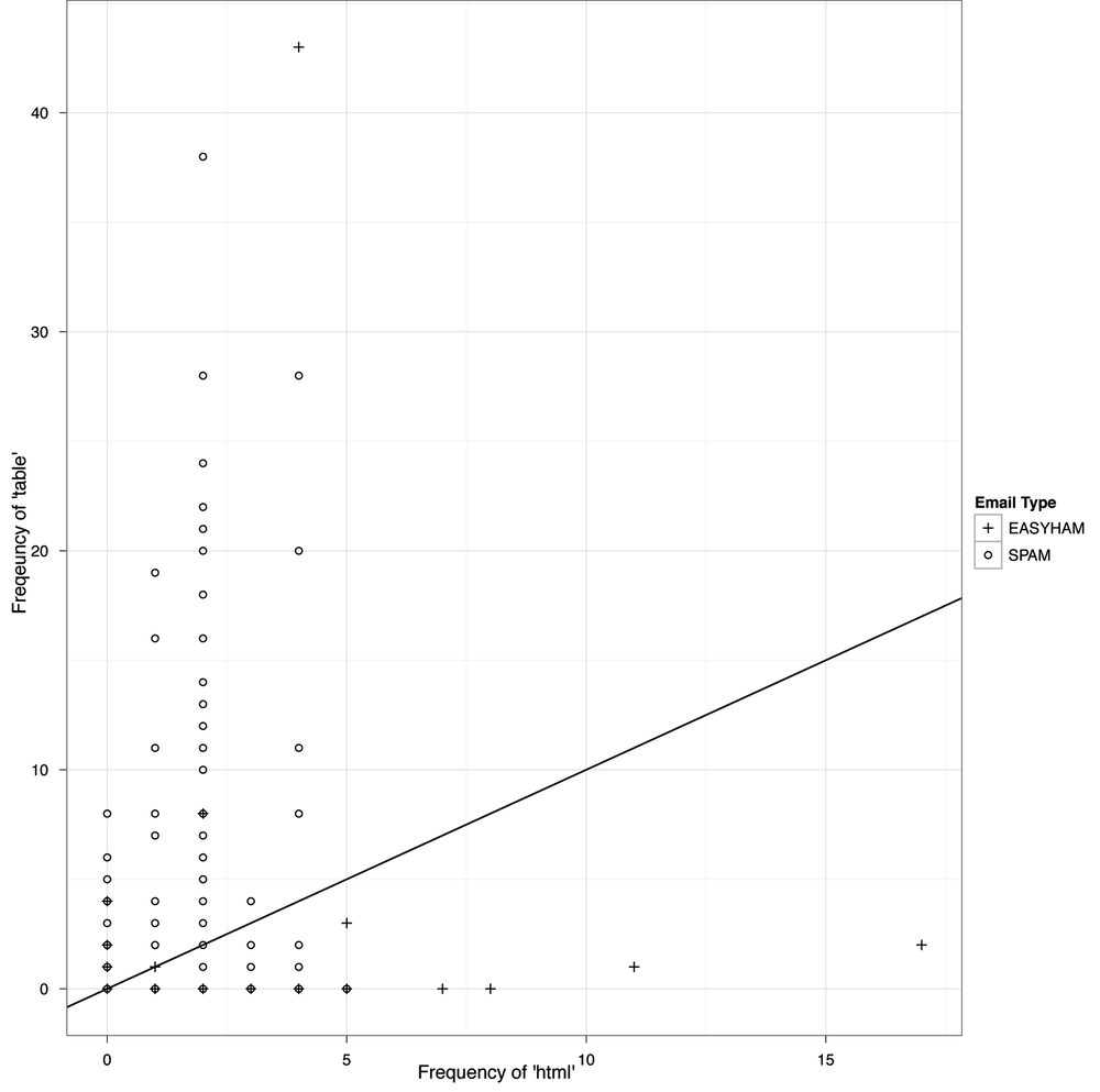
When working with text, historically the most important type of feature that’s been used is word count. If we think that the text of HTML tags are strong indicators of whether an email is spam, then we might pick terms like “html” and “table” and count how often they occur in one type of document versus the other. To show how this approach would work with the SpamAssassin public corpus, we’ve gone ahead and counted the number of times the terms “html” and “table” occurred. Table 3-1 shows the results.
For every email in our data set, we’ve also plotted the class
memberships in Figure 3-1. This plot isn’t
very informative, because too many of the data points in our data set
overlap. This sort of problem comes up quite often when you work with
data that contains only a few unique values for one or more of your
variables. As this is a recurring problem, there is a standard
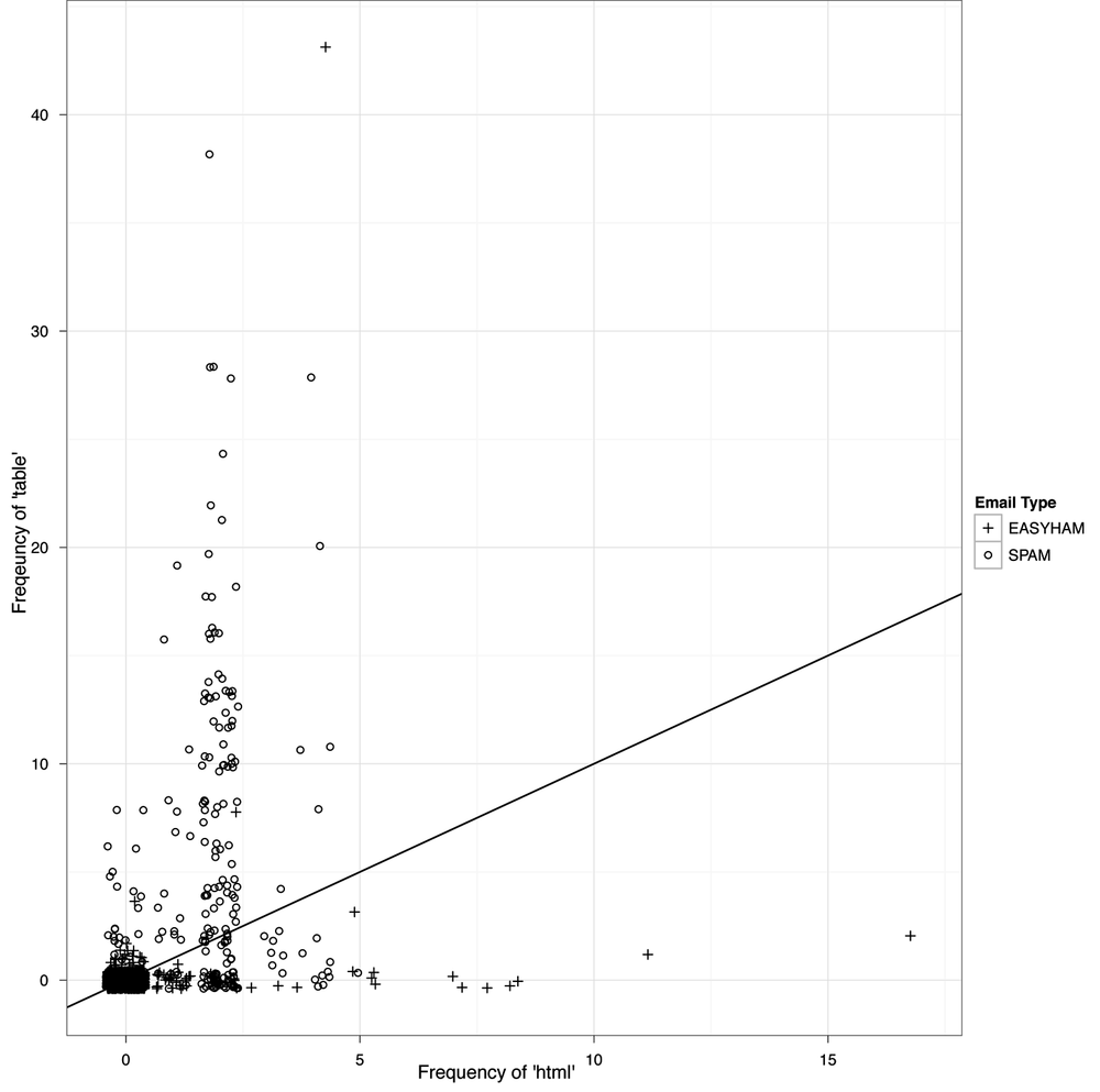
graphical solution: we simply add random noise to the values before we
plot. This noise will “separate out” the points to reduce the amount of
over-plotting. This addition of noise is called
jittering, and is very easy to produce in
ggplot2 (see Figure 3-2).
This last plot suggests that we could do a so-so job of deciding whether an email is spam simply by counting the number of times the terms “html” and “table” occur.
Note
The commands used to create the plots in Figures 3-1 and 3-2 begin at line 129 of the email_classify.R file in the code/ folder for this chapter.
In practice, we can do a much better job by using many more than just these two very obvious terms. In fact, for our final analysis we’ll use several thousand terms. Even though we’ll only use word-count data, we’ll still get a relatively accurate classification. In the real world, you’d want to use other features beyond word counts, such as falsified headers, IP or email black lists, etc., but here we only want to introduce the basics of text classification.
Before we can proceed, we should review some basic concepts of conditional probability and discuss how they relate to classifying a message based on its text.
At its core, text classification is a 20th-century application of the 18th-century concept of conditional probability. A conditional probability is the likelihood of observing one thing given some other thing that we already know about. For example, we might want to know the probability that a college student is female given that we already know the student’s major is computer science. This is something we can look up in survey results. According to a National Science Foundation survey in 2005, only 22% of undergraduate computer science majors were female SR08. But 51% of undergraduate science majors overall were female, so conditioning on being a computer science major lowers the chances of being a woman from 51% to 22%.
The text classification algorithm we’re going to use in this chapter, called the Naive Bayes classifier, looks for differences of this sort by searching through text for words that are either (a) noticeably more likely to occur in spam messages, or (b) noticeably more likely to occur in ham messages. When a word is noticeably more likely to occur in one context rather than the other, its occurrence can be diagnostic of whether a new message is spam or ham. The logic is simple: if you see a single word that’s more likely to occur in spam than ham, that’s evidence that the email as a whole is spam. If you see many words that are more likely to occur in spam than ham and very few words that are more likely to occur in ham than spam, that should be strong evidence that the email as a whole is spam.
Ultimately, our text classifier formalizes this intuition by computing (a) the probability of seeing the exact contents of an email conditioned on the email being assumed to be spam, and (b) the probability of seeing the same email’s contents conditioned on the email being assumed to be ham. If it’s much more likely that we would see the email in question if it were spam, we’ll declare it to be spam.
How much more likely a message needs to be to merit being labeled spam depends upon an additional piece of information: the base rate of seeing spam messages. This base rate information is usually called the prior. You can think of the prior in the following way: if most of the birds you see in the park are ducks and you hear a bird quacking one morning, it’s a pretty safe bet to assume that it’s a duck. But if you have never seen a duck in the park even once, it’s much riskier to assume that anything that quacks must be a duck. When working with email, the prior comes into play because the majority of email sent is spam, which means that even weak evidence that an email is spam can be sufficient to justify labeling it as spam.
In the following section we will elaborate on this logic in some detail as we write a spam classifier. To compute the probability of an email, we will assume that the occurrence counts for every word can be estimated in isolation from all of the other words. Formally, this amounts to an assumption often referred to as statistical independence. When we make this assumption without being certain that it’s correct, we say that our model is naive. Because we will also make use of base rate information about emails being spam, the model will be also called a Bayes model—in homage to the 18th-century mathematician who first described conditional probabilities. Taken together, these two traits make our model a Naive Bayes classifier.
As we mentioned earlier in this chapter, we will be using the SpamAssassin public corpus to both train and test our classifier. This data consists of labeled emails from three categories: “spam,” “easy ham,” and “hard ham.” As you’d expect, “hard ham” is more difficult to distinguish from spam than the easy stuff. For instance, hard ham messages often include HTML tags. Recall that one way to easily identify spam is by the presence of these tags. To more accurately classify hard ham, we will have to include more information from many more text features. Extracting these features requires some text mining of the email files and constitutes our initial step in creating a classifier.
All of our raw email files include the headers and the message text. A typical “easy ham” email looks like Example 3-1. You’ll note several features of this text that are of interest. First, the header contains a lot of information about where this email has come from. In fact, due to size constraints, we included only a portion of the total header in Example 3-1. And despite the fact that there is a lot of useful information contained in the headers, we will not be using any of this information in our classifier. Rather than focus on features contained in the transmission of the message, we are interested in how the contents of the messages themselves can help predict an email’s type. This is not to say that one should always ignore the header or any other information. In fact, all sophisticated modern spam filters utilize information contained in email message headers, such as whether portions of it appear to have been forged, whether the message is from a known spammer, or whether there are bits missing.
Because we are focusing on only the email message body, we need to extract this text from the message files. If you explore some of the message files contained in this exercise, you will notice that the email message always begins after the first full line break in the email file. In Example 3-1, we see that the sentence “Hello, have you seen and discussed this article and his approach?” comes directly after the first line break. To begin building our classifier, we must first create R functions that can access the files and extract the message text by taking advantage of this text convention.
Example 3-1. Typical “easy ham” email
........................................................
Received: from usw-sf-list1-b.sourceforge.net ([10.3.1.13]
helo=usw-sf-list1.sourceforge.net) by usw-sf-list2.sourceforge.net with
esmtp (Exim 3.31-VA-mm2 #1 (Debian)) id 17hsof-00042r-00; Thu,
22 Aug 2002 07:20:05 -0700
Received: from vivi.uptime.at ([62.116.87.11] helo=mail.uptime.at) by
usw-sf-list1.sourceforge.net with esmtp (Exim 3.31-VA-mm2 #1 (Debian)) id
17hsoM-0000Ge-00 for <spamassassin-devel@lists.sourceforge.net>;
Thu, 22 Aug 2002 07:19:47 -0700
Received: from [192.168.0.4] (chello062178142216.4.14.vie.surfer.at
[62.178.142.216]) (authenticated bits=0) by mail.uptime.at (8.12.5/8.12.5)
with ESMTP id g7MEI7Vp022036 for
<spamassassin-devel@lists.sourceforge.net>; Thu, 22 Aug 2002 16:18:07
+0200
From: David H=?ISO-8859-1?B?9g==?=hn <dh@uptime.at>
To: <spamassassin-devel@example.sourceforge.net>
Message-Id: <B98ABFA4.1F87%dh@uptime.at>
MIME-Version: 1.0
X-Trusted: YES
X-From-Laptop: YES
Content-Type: text/plain; charset="US-ASCII”
Content-Transfer-Encoding: 7bit
X-Mailscanner: Nothing found, baby
Subject: [SAdev] Interesting approach to Spam handling..
Sender: spamassassin-devel-admin@example.sourceforge.net
Errors-To: spamassassin-devel-admin@example.sourceforge.net
X-Beenthere: spamassassin-devel@example.sourceforge.net
X-Mailman-Version: 2.0.9-sf.net
Precedence: bulk
List-Help: <mailto:spamassassin-devel-request@example.sourceforge.net?subject=help>
List-Post: <mailto:spamassassin-devel@example.sourceforge.net>
List-Subscribe: <https://example.sourceforge.net/lists/listinfo/spamassassin-devel>,
<mailto:spamassassin-devel-request@lists.sourceforge.net?subject=subscribe>
List-Id: SpamAssassin Developers <spamassassin-devel.example.sourceforge.net>
List-Unsubscribe: <https://example.sourceforge.net/lists/listinfo/spamassassin-devel>,
<mailto:spamassassin-devel-request@lists.sourceforge.net?subject=unsubscribe>
List-Archive: <http://www.geocrawler.com/redir-sf.php3?list=spamassassin-devel>
X-Original-Date: Thu, 22 Aug 2002 16:19:48 +0200
Date: Thu, 22 Aug 2002 16:19:48 +0200
Hello, have you seen and discussed this article and his approach?
Thank you
http://www.paulgraham.com/spam.html
-- “Hell, there are no rules here-- we’re trying to accomplish something.”
-- Thomas Alva Edison
-------------------------------------------------------
This sf.net email is sponsored by: OSDN - Tired of that same old
cell phone? Get a new here for FREE!
https://www.inphonic.com/r.asp?r=sourceforge1&refcode1=vs3390
_______________________________________________
Spamassassin-devel mailing list
Spamassassin-devel@lists.sourceforge.net
https://lists.sourceforge.net/lists/listinfo/spamassassin-devel
Note
The “null line” separating the header from the body of an email is part of the protocol definition. For reference, see RFC822: http://tools.ietf.org/html/frc822.
As is always the case, the first thing to do is to load in
the libraries we will use for this exercise. For text classification, we
will be using the tm package, which
stands for text mining. Once we have built our
classifier and tested it, we will use the ggplot2 package to visually analyze the
results. Another important initial step is to set the path variables for
all of the email files. As mentioned, we have three types of messages:
easy ham, hard ham, and spam. In the data file directory for this
exercise, you will notice that there are two separate sets of file
folders for each type of message. We will use the first set of files to train the classifier
and the second set to test it.
library(tm)
library(ggplot2)

spam.path <- "data/spam/"
spam2.path <- "data/spam_2/"
easyham.path <- "data/easy_ham/"
easyham2.path <- "data/easy_ham_2/"
hardham.path <- "data/hard_ham/"
hardham2.path <- "data/hard_ham_2/"
With the requisite packages loaded and the path variables set, we can begin building up our knowledge about the type of terms used in spam and ham by creating text corpuses from both sets of files. To do this, we will write a function that opens each file, finds the first line break, and returns the text below that break as a character vector with a single text element.
get.msg <- function(path) {
    con <- file(path, open="rt", encoding="latin1")
    text <- readLines(con)
    # The message always begins after the first full line break
    msg <- text[seq(which(text=="")[1]+1,length(text),1)]
    close(con)
    return(paste(msg, collapse="\n"))
}
The R language performs file I/O in a very similar way to many
other programming languages. The function shown here takes a file path
as a string and opens that file in rt mode, which
stands for read as text. Also notice that the
coding is latin1. This is because many of the email
messages contain non-ASCII characters, and this encoding will allow us
to use these files. The readLines function
will return each line of text in the file connection as a separate
element of a character vector. As such, once we have read in all of the
lines, we want to locate the first empty element of the text and then
extract all the elements afterward. Once we have the email message as a
character vector, we’ll close the file connection and then collapse the
vector into a single character element using the paste function and
\n (new line) for the collapse argument.
To train our classifier, we will need to get the email messages
from all of our spam and ham emails. One approach is to create a vector
containing all of the messages, such that each element of the vector is
a single email. The most straightforward way to accomplish this in R is to
use an apply function with our newly
created get.msg function.
spam.docs <- dir(spam.path)
spam.docs <- spam.docs[which(spam.docs!="cmds")]
all.spam <- sapply(spam.docs, function(p) get.msg(paste(spam.path,p,sep="")))
For the spam email, we begin by getting a listing of all of
the filenames in the data/spam directory using the
dir function. This directory—and all
of the directories holding email data—also contain a cmds file, which is simply a long list of Unix
base commands to move files in these directories. This is not something
we want to include in our training data, so we ignore it by keeping only
those files that do not have cmds as
a filename. Now spam.docs is a
character vector containing all of the filenames for the spam messages
we will use to train our classifier.
To create our vector of spam messages, we use the sapply function, which will apply get.msg to all of the spam filenames and
construct a vector of messages from the returned text.
Note
Note that we have to pass an anonymous function to sapply in order to concatenate the
filename with the appropriate directory path using the paste function. This is a very common
construction in R.
Once you have executed this series of commands, you can use
head(all.spam) to inspect the
results. You will note that the name of each vector element corresponds
to the filename. This is one of the advantages of using sapply.
The next step is to create a text corpus from our vector of emails
using the functions provided by the tm package. Once we have the text represented
as a corpus, we can manipulate the terms in the messages to begin
building our feature set for the spam classifier. A huge advantage of
the tm package is that much of the
heavy lifting needed to clean and normalize the text is hidden from
view. What we will accomplish in a few lines of R code would take many
lines of string processing if we had to perform these operations
ourselves in a lower-level language.
One way of quantifying the frequency of terms in our spam
email is to construct a term document matrix (TDM).
As the name suggests, a TDM is an N×M matrix in which the terms found
among all of the documents in a given corpus define the rows and all of
the documents in the corpus define the columns. The [i, j]
cell of this matrix corresponds to the number of times term
i was found in document j.
As before, we will define a simple function, get.tdm, that will take a vector of email
messages and return a TDM:
get.tdm <- function(doc.vec) {
    doc.corpus <- Corpus(VectorSource(doc.vec))
    control <- list(stopwords=TRUE, removePunctuation=TRUE, removeNumbers=TRUE,
        minDocFreq=2)
    doc.dtm <- TermDocumentMatrix(doc.corpus, control)
    return(doc.dtm)
}

spam.tdm <- get.tdm(all.spam)
The tm package allows you to
construct a corpus in several ways. In our case, we will construct the corpus from a vector of
emails, so we will use the VectorSource function. To see the various
other source types that can be used, enter ?getSources at the R console. As is often the
case when working with tm, once we
have loaded our source text, we will use the Corpus
function in conjunction with VectorSource to create a corpus object. Before
we can proceed to creating the TDM, however, we must tell tm how we want it to clean and normalize the
text. To do this we use a control, which is a special list of options
specifying how to distill the text.
For this exercise we will use four options. First, we set stopwords=TRUE, which tells tm to remove 488 common English stop words
from all of the documents. To see the list, type stopwords() at the R console. Next, we set
removePunctuation and removeNumbers to TRUE, which are fairly self-explanatory and
are used to reduce the noise associated with these characters—especially
because many of our documents contain HTML tags. Finally, we set
minDocFreq=2, which will ensure that
only terms appearing more than once in the corpus will end up in the
rows of the TDM.
We now have processed the spam emails to the point where we can begin building our classifier. Specifically, we can use the TDM to build a set of training data for spam. Within the context of R, a good approach to doing this is to construct a data frame that contains all of the observed probabilities for each term, given that we know it is spam. Just as we did with our female computer science major example, we need to train our classifier to know the probability that an email is spam, given the observation of some term.
spam.matrix <- as.matrix(spam.tdm)
spam.counts <- rowSums(spam.matrix)
spam.df <- data.frame(cbind(names(spam.counts),
     as.numeric(spam.counts)), stringsAsFactors=FALSE)
names(spam.df) <- c("term","frequency")
spam.df$frequency <- as.numeric(spam.df$frequency)

spam.occurrence <- sapply(1:nrow(spam.matrix),
     function(i) {length(which(spam.matrix[i,] > 0))/ncol(spam.matrix)})
spam.density <- spam.df$frequency/sum(spam.df$frequency)

spam.df <- transform(spam.df, density=spam.density,
     occurrence=spam.occurrence)
To create this data frame, we must first convert the TDM
object to a standard R matrix using the as.matrix command. Then, using the rowSums
command, we can create a vector that contains the total frequency counts
for each term across all documents. Because we will use the data.frame function to
combine a character vector with a numeric vector, by
default R will convert these vectors to a common representation. The
frequency counts can be represented as characters, and so they will be
converted, which means we must be mindful to set stringsAsFactors=FALSE. Next, we will do some
housekeeping to set the column names and convert the frequency counts
back to a numeric vector.
With the next two steps, we will generate the critical
training data. First, we calculate the percentage of documents in which
a given term occurs. We do this by passing every row through an
anonymous function call via sapply,
which counts the number of cells with a positive element and then
divides the total by the number of columns in the TDM—i.e., by the
number of documents in the spam corpus. Second, we calculate the
frequency of each word within the entire corpus. (We will not use the
frequency information for classification, but it will be useful to see
how these numbers compare when we consider how certain words might be
affecting our results.)
In the final step, we add the spam.occurrence and spam.density vectors to the data frame using
the transform function. We have now
generated the training data for spam classification!
Let’s check the data and see which terms are the strongest
indicators of spam given our training data. To do this, we sort spam.df by the occurrence column and inspect its head:
head(spam.df[with(spam.df, order(-occurrence)),])
      term frequency     density occurrence
2122  html       377 0.005665595      0.338
538   body       324 0.004869105      0.298
4313 table      1182 0.017763217      0.284
1435 email       661 0.009933576      0.262
1736  font       867 0.013029365      0.262
1942  head       254 0.003817138      0.246
As we have mentioned repeatedly, HTML tags appear to be the
strongest text features associated with spam. Over 30% of the messages
in the spam training data contain the term html, as well as other common HTML-related
terms, such as body, table, font, and head. Note, however, that these terms are not
the most frequent by raw count. You can see this for yourself by
replacing -occurrence with -frequency in the preceding statement. This is
very important in terms of how we define our classifier. If we used raw
count data and the subsequent densities as our training data, we might
be over weighting certain kinds of spam—specifically, spam that contains
HTML tables. However, we know that not all spam messages are constructed
this way. As such, a better approach is to define the conditional
probability of a message being spam based on how many messages contain
the term.
Now that we have the spam training data, we need to balance it with the ham training data. As part of the exercise, we will build this training data using only the easy ham messages. Of course, it would be possible to incorporate the hard ham messages into the training set; in fact, that would be advisable if we were building a production system. But within the context of this exercise, it’s helpful to see how well a text classifier will work if trained using only a small corpus of easily classified documents.
We will construct the ham training data in exactly the same way we
did the spam, and therefore we will not reprint those commands here. The
only way this step differs from generating the spam training data is
that we use only the first 500 email messages in the data/easy_ham folder.
You may note that there are actually 2,500 ham emails in this directory. So why are we ignoring four-fifths of the data? When we construct our first classifier, we will assume that each message has an equal probability of being ham or spam. As such, it is good practice to ensure that our training data reflects our assumptions. We only have 500 spam messages, so we will limit or ham training set to 500 messages as well.
Note
To see how we limited the ham training data in this way, see line 102 in the email_classify.R file for this chapter.
Once the ham training data has been constructed, we can inspect it just as we did the spam for comparison:
head(easyham.df[with(easyham.df, order(-occurrence)),])
       term frequency     density occurrence
3553  yahoo       185 0.008712853      0.180
966    dont       141 0.006640607      0.090
2343 people       183 0.008618660      0.086
1871  linux       159 0.007488344      0.084
1876   list       103 0.004850940      0.078
3240   time        91 0.004285782      0.064
The first thing you will notice in the ham training data is that the terms are much more sparsely distributed among the emails. The term that occurs in the most documents, “yahoo,” does so in only 18% of them. The other terms all occur in less than 10% of the documents. Compare this to the top spam terms, which all occur in over 24% of the spam emails. Already we can begin to see how this variation will allow us to separate spam from ham. If a message contains just one or two terms strongly associated with spam, it will take a lot of nonspam words for the message to be classified as ham. With both training sets defined, we are now ready to complete our classifier and test it!
We want to define a classifier that will take an email message file and calculate the probability that it is spam or ham. Fortunately, we have already created most of the functions and generated the data needed to perform this calculation. Before we can proceed, however, there is one critical complication that we must consider.
We need to decide how to handle terms in new emails that match terms in our training set and how to handle terms that do not match terms in our training set (see Figure 3-3). To calculate the probability that an email message is spam or ham, we will need to find the terms that are common between the training data and the message in question. We can then use the probabilities associated with these terms to calculate the conditional probability that a message is of the training data’s type. This is fairly straightforward, but what do we do with the terms from the email being classified that are not in our training data?
To calculate the conditional probability of a message, we
combine the probabilities of each term in the training data by taking
their product. For example, if the frequency of seeing html in a spam message is 0.30 and the
frequency of seeing table in a spam
message is 0.10, then we’ll say that the probability of seeing both in
a spam message is 0.30 × 0.10 = 0.03. But for those terms in the email
that are not in our training data, we have no information about their
frequency in either spam or ham messages. One possible solution would
be to assume that because we have not seen a term yet, its probability
of occurring in a certain class is zero. This, however, is very
misguided. First, it is foolish to assume that we will never see a
term in the entire universe of spam and ham simply because we have not
yet seen it. Moreover, because we calculate conditional probabilities
using products, if we assigned a zero probability to terms not in our
training data, elementary arithmetic tells us that we would calculate
zero as the probability of most messages, because we would be
multiplying all the other probabilities by zero every time we
encountered an unknown term. This would cause catastrophic results for our classifier
because many, or even all, messages would be incorrectly assigned a zero probability
of being either spam or ham.
Researchers have come up with many clever ways of trying to get
around this problem, such as drawing a random probability from some
distribution or using natural language processing (NLP) techniques to
estimate the “spamminess” of a term given its context. For our
purposes, we will use a very simple rule: assign a very small
probability to terms that are not in the training set. This is, in
fact, a common way of dealing with missing terms in simple text
classifiers, and for our purposes it will serve just fine. In this
exercise, by default we will set this probability to 0.0001%, or
one-ten-thousandth of a percent, which is sufficiently small for this
data set. Finally, because we are assuming that all emails are equally
likely to be ham or spam, we set our default prior belief that an
email is of some type to 50%. In order to return to this problem
later, however, we construct the classify.email function such that the prior
can be varied.
Warning
Be wary of always using 0.0001% for terms not in a training set. We are using it in this example, but in others it may be too large or too small, in which case the system you build will not work at all!
classify.email <- function(path, training.df, prior=0.5, c=1e-6) {
    msg <- get.msg(path)
    msg.tdm <- get.tdm(msg)
    msg.freq <- rowSums(as.matrix(msg.tdm))
    # Find intersections of words
    msg.match <- intersect(names(msg.freq), training.df$term)
    if(length(msg.match) < 1) {
        return(prior*c^(length(msg.freq)))
    }
    else {
        match.probs <- training.df$occurrence[match(msg.match, training.df$term)]
        return(prior * prod(match.probs) * c^(length(msg.freq)-length(msg.match)))
    }
}
You will notice that the first three steps of the classify.email function proceed just as our
training phase did. We must extract the message text with get.msg, turn it into a TDM with get.tdm, and finally calculate the frequency
of terms with rowSums. Next, we
need to find how the terms in the email message intersect with the
terms in our training data, as depicted in Figure 3-3. To do so, we use the
intersect command, passing the
terms found in the email message and those in the training data. What
will be returned are those terms in the gray shaded area of Figure 3-3.
The final step of the classification is to determine whether any of the words in the email message are present in the training set, and if so, we use them to calculate the probability that this message is of the class in question.
Assume for now that we are attempting to determine if this email
message is spam. msg.match will
contain all of the terms from the email message in our spam training
data, spam.df. If that intersection
is empty, then the length of msg.match will be less than zero, and we can
update our prior only by multiplying it with the product of the number
of terms in the email with our tiny probability value: c. The result will be a tiny probability of
assigning the spam label to the email.
Conversely, if this intersection is not empty, we need to find
those terms from the email in our training data and look up their
occurrence probabilities. We use the match function to do the lookup, which will
return the term’s element position in the term column of our training data. We use
these element positions to return the corresponding probabilities from
the occurrence column, and return
those values to match.probs. We
then calculate the product of these values and
combine it with our prior belief about the email being spam with the
term probabilities and the probabilities of any missing terms. The
result is our Bayesian estimate for the probability that a message is
spam given the matching terms in our training data.
As an initial test, we will use our training data from the spam and easy ham messages to classify hard ham emails. We know that all of these emails are ham, so ideally our classifier will assign a higher probability of being ham to all of these messages. We also know, however, that hard ham messages are “hard” to classify because they contain terms that are also associated with spam. Now let’s see how our simple classifier does!
hardham.docs <- dir(hardham.path)
hardham.docs <- hardham.docs[which(hardham.docs != "cmds")]

hardham.spamtest <- sapply(hardham.docs,
    function(p) classify.email(paste(hardham.path, p, sep=""),
    training.df=spam.df))

hardham.hamtest <- sapply(hardham.docs,
    function(p) classify.email(paste(hardham.path, p, sep=""),
    training.df=easyham.df))

hardham.res <- ifelse(hardham.spamtest > hardham.hamtest, TRUE, FALSE)
summary(hardham.res)
Just as before, we need to get all of the file paths in order,
and then we can test the classifier for all hard ham messages by
wrapping both a spam test and ham test in sapply calls. The vectors hardham.spamtest and hardham.hamtest contain the conditional probability calculations for
each hard ham email of being either spam or ham given the appropriate
training data. We then use the ifelse command to compare the probabilities
in each vector. If the value in hardham.spamtest is greater than that in
hardham.hamtest, then the
classifier has classified the message as spam; otherwise, it is ham.
Finally, we use the summary command
to inspect the results, listed in Table 3-2.
Table 3-2. Testing our classifier against “hard ham”
| Email type | Number classified as ham | Number classified as spam |
|---|---|---|
| Hard ham | 184 | 65 |
Congratulations! You’ve written your first classifier, and it did fairly well at identifying hard ham as nonspam. In this case, we have approximately a 26% false-positive rate. That is, about one-quarter of the hard ham emails are incorrectly identified as spam. You may think this is poor performance, and in production we would not want to offer an email platform with these results, but considering how simple our classifier is, it is doing quite well. Of course, a better test is to see how the classifier performs against not only hard ham, but also easy ham and spam.
The first step is to build a simple function that will do the the probability comparison we did in the previous section all at once for all emails.
spam.classifier <- function(path) {
    pr.spam <- classify.email(path, spam.df)
    pr.ham <- classify.email(path, easyham.df)
    return(c(pr.spam, pr.ham, ifelse(pr.spam > pr.ham, 1, 0)))
}
For simplicity’s sake, the spam.classifier function will determine
whether an email is spam based on the spam.df and easyham.df training data. If the probability
that a message is spam is greater than its probability of being ham,
it returns one; otherwise, it returns zero.
As a final step in this exercise, we will test the second sets
of spam, easy ham, and hard ham using our simple classifier. These
steps proceed exactly as they did in previous sections: wrapping the
spam.classifier function in an
lapply function, passing email file
paths, and building a data frame. As such, we will not reproduce these
function calls here, but you are encouraged to reference the email_classifier.R file starting at line 158
to see how this is done.
The new data frame contains the likelihoods of being either spam
or ham, the classification, and the email type for each message in all
three data sets. The new data set is called class.df, and we can use the head command to inspect its contents:
head(class.df)
        Pr.SPAM        Pr.HAM Class    Type
1 2.712076e-307 1.248948e-282 FALSE EASYHAM
2  9.463296e-84  1.492094e-58 FALSE EASYHAM
3  1.276065e-59  3.264752e-36 FALSE EASYHAM
4  0.000000e+00 3.539486e-319 FALSE EASYHAM
5  2.342400e-26  3.294720e-17 FALSE EASYHAM
6 2.968972e-314 1.858238e-260 FALSE EASYHAM
From the first six entries, it seems the classifier has done well, but let’s calculate the false-positive and false-negative rates for the classifier across all data sets. To do this, we will construct an N × M matrix of our results, where the rows are the actual classification types and the columns are the predicted types. Because we have three types of email being classified into two types, our confusion matrix will have three rows and two columns (as shown in Table 3-3). The columns will be the percent predicted as ham or spam, and if our classifier works perfectly, the columns will read [1,1,0] and [0,0,1], respectively.
Table 3-3. Matrix for classifier results
| Email type | % Classified as ham | % Classified as spam |
|---|---|---|
| Easy ham | 0.78 | 0.22 |
| Hard ham | 0.73 | 0.27 |
| Spam | 0.15 | 0.85 |
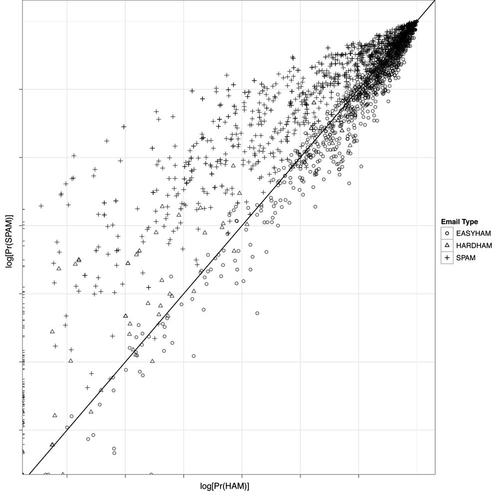
Unfortunately, we did not write a perfect classifier, but the results are still quite good. Similar to our initial test, we get about a 25% false-positive rate, with our classifier doing slightly better on easy ham than the hard stuff. On the other hand, the false-negative rate is much lower at only 15%. To get a better sense of how our classifier fared, we can plot the results using a scatterplot, with the predicted probabilities of being ham on the x-axis and spam on the y-axis.
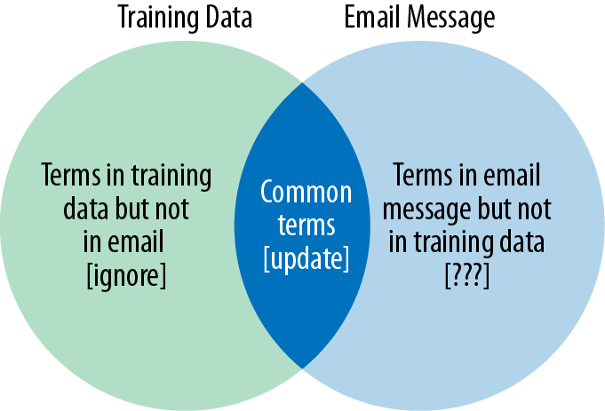
Figure 3-5 shows this scatterplot in log-log scale. A log transformation is done because many of the predicted probabilities are very tiny, while others are not. With this high degree of variance, it is difficult to compare the results directly. Taking logs is a simple way of altering the visual scale to more easily compare values.
We have also added a simple decision boundary to the plots where y = x, or a perfect linear relationship. This is done because our classifier compares the two predicted probabilities and determines the email’s type based on whether the probability of being spam is greater than that of ham. All dots above the black diagonal line, therefore, should be spam, and all those below should be ham. As you can see, this is not the case—but there is considerable clustering of message types.
Figure 3-5 also gives some intuition about how the classifier is underperforming with respect to false-positives. There appear to be two general ways it is failing. First, there are many hard ham messages that have a positive probability of being spam but a near-zero probability of being ham. These are the points pressed up against the y-axis. Second, there are both easy and hard ham messages that have a much higher relative probability of being ham. Both of these observations may indicate a weak training data set for ham emails, as there are clearly many more terms that should be associated with ham that currently are not.
In this chapter we have introduced the idea of text classification. To do this, we constructed a very simple Bayesian classifier using a minimal number of assumptions and features. At its core, this type of classification is an application of classic conditional probability theory in a contemporary context. Despite the fact that we trained our classifier with only a fraction of the total available data, this simple method performed reasonably well.
That said, the false-positive and false-negative rates found in the test data are far too high for any production spam filter. As we mentioned throughout this chapter, there are many simple tweaks we could apply to improve the results of the current model. For example, our approach assumes a priori that each email has an equal probability of being ham or spam. In practice, however, we know that this relationship is actually much closer to 80%–20% ham-to-spam. One way we might improve results, then, would be to simply alter our prior beliefs to reflect this fact and recalculate the predicted probabilities.
spam.classifier<-function(path) {
    pr.spam<-classify.email(path, spam.df, prior=0.2)
    pr.ham<-classify.email(path, easyham.df, prior=0.8)
    return(c(pr.spam, pr.ham, ifelse(pr.spam > pr.ham, 1, 0)))
}
You’ll remember that we left the prior parameter as something that could vary
in the classify.email function, so
we now only need to make the simple change to spam.classify
shown in the preceding example. We could rerun the classifier
now and compare the results, and we encourage you to do so. These new
assumptions, however, violate the distributions of ham and spam
messages in our training data. To be more accurate, we should go back
and retrain the classifier with the complete easy ham data set. Recall
that we limited our original ham training data to only the first 500
messages so that our training data would reflect the Bayesian
assumptions. In that vein, we must incorporate the full data set in
order to reflect our new assumptions.
When we rerun the classifier with the new easyham.df and classify.email parameterization, we see a
notable improvement in performance on false-positives (see Table 3-4).
Table 3-4. Matrix for improved classifier results
| Email type | % Classified as ham | % Classified as spam |
|---|---|---|
| Easy ham | 0.90 | 0.10 |
| Hard ham | 0.82 | 0.18 |
| Spam | 0.18 | 0.82 |
With these simple changes, we have reduced our false-positive rate by more than 50%! What is interesting, however, is that by improving performance in this way, our false-negative results suffer. In essence, what we are doing is moving the decision boundaries (recall Example 3-1). By doing so, we are explicitly trading off false positives for improvement in false negatives. This is an excellent example of why model specification is critical, and how each assumption and feature choice can affect all results.
In the following chapter we will expand our view of classification beyond the simple binary—this or that—example in this exercise. As we mentioned at the outset, often it is difficult or impossible to classify observations based on a single decision boundary. In the next chapter we will explore how to rank emails based on features that are associated with higher priority. What remain important as we increase the spectrum of classification tasks are the features we decide to include in our model. As you’ll see next, the data may limit feature selection, which can have a serious impact on our model design.