In the last chapter, we saw how we could use simple correlational techniques to create a measure of similarity between the members of Congress based on their voting records. In this chapter, we’re going to talk about how you can use those same sort of similarity metrics to recommend items to a website’s users.

The algorithm we’ll use is called k-nearest neighbors. It’s arguably the most intuitive of all the machine learning algorithms that we present in this book. Indeed, the simplest form of k-nearest neighbors is the sort of algorithm most people would spontaneously invent if asked to make recommendations using similarity data: they’d recommend the song that’s closest to the songs a user already likes, but not yet in that list. That intuition is essentially a 1-nearest neighbor algorithm. The full k-nearest neighbor algorithm amounts to a generalization of this intuition where you draw on more than one data point before making a recommendation.

The full k-nearest neighbors algorithm works much in the way some of us ask for recommendations from our friends. First, we start with people whose taste we feel we share, and then we ask a bunch of them to recommend something to us. If many of them recommend the same thing, we deduce that we’ll like it as well.

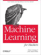
How can we take that intuition and transform it into something algorithmic? Before we work on making recommendations based on real data, let’s start with something simpler: classifying points into two categories. If you remember how we first motivated the problem of classifying spam back in Chapter 3, you’ll remember a picture like the one shown in Figure 10-1.

Figure 10-1. Classification problem with a linear decision boundary

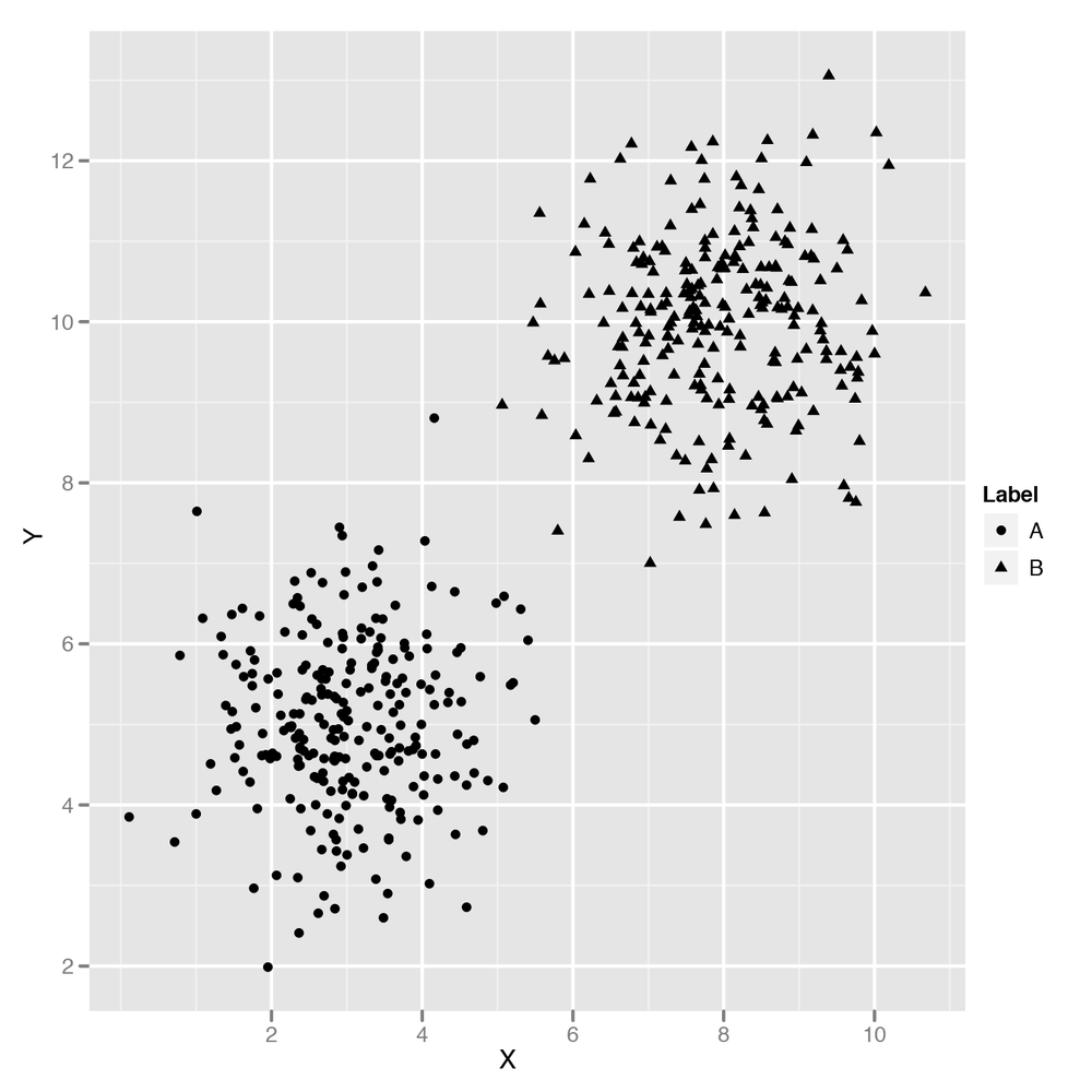
As we explained, you can use logistic regression through the glm function to split those points using a single line that we called the decision boundary. At the same time that we explained how to use logistic regression, we also said that there were problems like the one shown in Figure 10-2 that can’t be solved using a simple linear decision boundary.

Figure 10-2. Classification problem with a nonlinear decision boundary

How could you try to build a classifier that would match a more complicated decision boundary like the one shown in Figure 10-2? You could try coming up with a nonlinear method; the kernel trick, which we’ll discuss in Chapter 12, is an example of this approach.

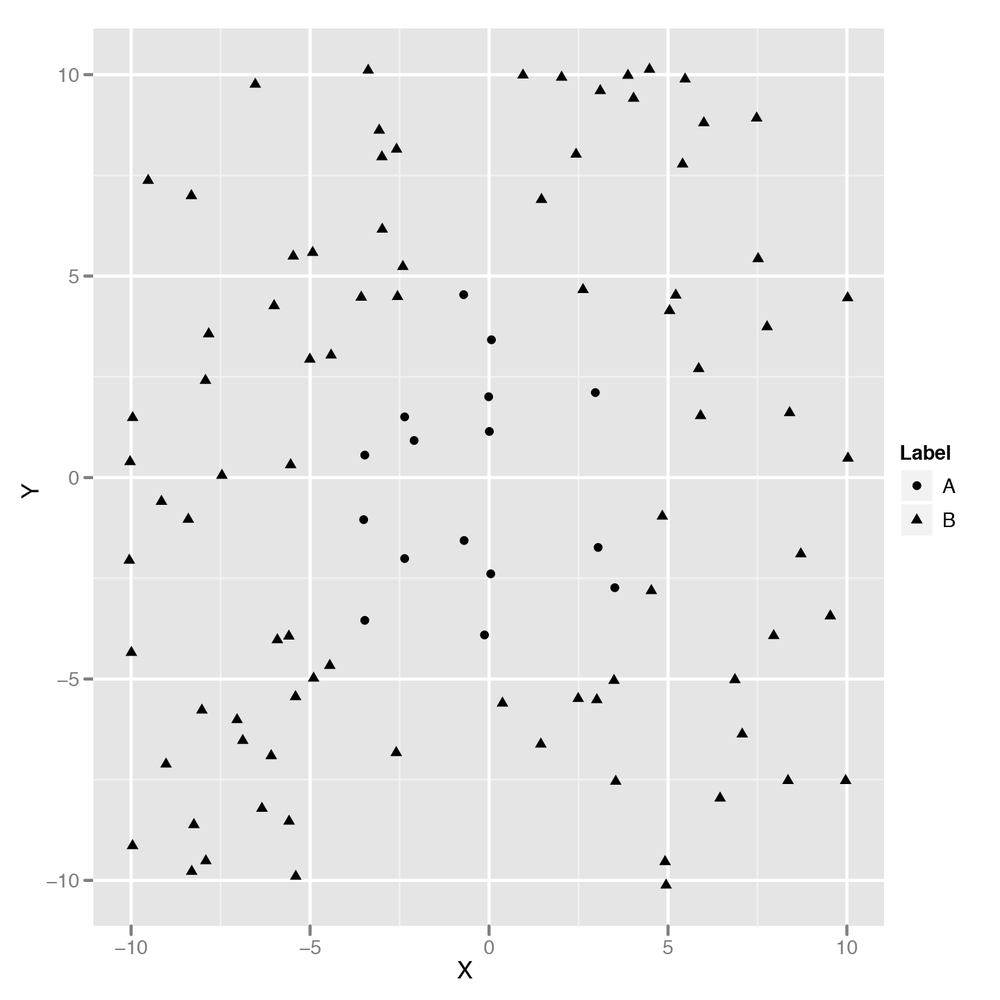
Another approach would be to use the points nearest the point you’re trying to classify to make your guess. You could, for example, draw a circle around the point you’re looking at and then decide on a classification based on the points within that circle. Figure 10-3 shows just such an approach, which we’ll quickly call the “Grassroots Democracy” algorithm.

Figure 10-3. The “Grassroots Democracy” algorithm

This algorithm is actually pretty usable, but it has one noticeable flaw: we have to pick a radius for the circle we’ll use to define “local” points. If all of your data points have their neighbors at roughly the same distance, this won’t be a problem. But if some points have many close neighbors while others have almost none, you’ll end up picking a circle that’s so big it extends well past the decision boundaries for some points. What can we do to work around this problem? The obvious solution is to avoid using a circle to define a point’s neighbors and instead look at the k-closest points. Those points are called the k-nearest neighbors. Once we have them, we can then look at their classifications and use majority rule to decide on a class for our new point. Let’s build code to do just that now.

First, we’ll read in our data set:

df <- read.csv('data/example_data.csv')

head(df)
#         X        Y Label
#1 2.373546 5.398106     0
#2 3.183643 4.387974     0
#3 2.164371 5.341120     0
#4 4.595281 3.870637     0
#5 3.329508 6.433024     0
#6 2.179532 6.980400     0

Then we need to compute the distance between each of the points in our data set. We’ll store this information in a distance matrix, which is a simple 2D array in which the distance between point i and point j is found at the array entry distance.matrix[i, j]. The following code produces this distance matrix using the Euclidean distance formula:

distance.matrix <- function(df)
{
  distance <- matrix(rep(NA, nrow(df) ^ 2), nrow = nrow(df))

  for (i in 1:nrow(df))
  {
    for (j in 1:nrow(df))
    {
      distance[i, j] <- sqrt((df[i, 'X'] - df[j, 'X']) ^ 2 + (df[i, 'Y'] - df[j, 'Y']) 
                              ^ 2)
    }
  }

  return(distance)
}

Once we have the distance matrix, we need a function that will return the k-nearest neighbors for a point. It’s actually easy to implement this in R because you can simply look at the ith row of the distance matrix to find how far all the other points are from your input point. Once you sort this row, you have a list of the neighbors ordered by their distance from the input point. Just select the first k entries after ignoring the input point (which should always be the very first point in the distance matrix), and you’ll have the k-nearest neighbors of your input point.

k.nearest.neighbors <- function(i, distance, k = 5)
{
  return(order(distance[i, ])[2:(k + 1)])
}

Once you’ve done that, we’ll build a knn function that takes a data frame and a value for k and then produces predictions for each point in the data frame. Our function isn’t very general, because we’re assuming that the class labels are found in a column called Label, but this is just a quick exercise to see how the algorithm works. There are already implementations of k-nearest neighbors in R that you can use for practical work, and we’ll discuss one in just a moment.

knn <- function(df, k = 5)
{
  distance <- distance.matrix(df)

  predictions <- rep(NA, nrow(df))

  for (i in 1:nrow(df))
  {
    indices <- k.nearest.neighbors(i, distance, k = k)
    predictions[i] <- ifelse(mean(df[indices, 'Label']) > 0.5, 1, 0)
  }

  return(predictions)
}

As you can see, we’ve used majority rules voting to make our predictions by taking the mean label and then thresholding at 0.5. Calling this function returns a vector of predictions, so we append those to our data frame and then assess our performance:

df <- transform(df, kNNPredictions = knn(df))

sum(with(df, Label != kNNPredictions))
#[1] 7

nrow(df)
#[1] 100

We’ve incorrectly predicted the labels for 7 points out of 100, so we’re correct 93% of the time. That’s not bad performance for such a simple algorithm. Now that we’ve explained how the k-nearest neighbors (kNN) algorithm works, we’ll apply kNN to some real data about the usage of R packages.

But before we do that, let’s quickly show you how to use a black-box implementation of kNN for your own projects:

rm('knn') # In case you still have our implementation in memory.
library('class')

df <- read.csv('data/example_data.csv')

n <- nrow(df)

set.seed(1)
indices <- sort(sample(1:n, n * (1 / 2)))

training.x <- df[indices, 1:2]
test.x <- df[-indices, 1:2]
training.y <- df[indices, 3]
test.y <- df[-indices, 3]

predicted.y <- knn(training.x, test.x, training.y, k = 5)
sum(predicted.y != test.y)
#[1] 7

length(test.y)
#[1] 50

Here we’ve tested the knn function from the class package using cross-validation. Amazingly, we get exactly 7 labels wrong here as well, but the test set has only 50 examples, so we’re only achieving 86% accuracy. That’s still pretty good, though. Let’s just show you how a logistic model would have worked to give you a point of comparison:

logit.model <- glm(Label ~ X + Y, data = df[indices, ])

predictions <- as.numeric(predict(logit.model, newdata = df[-indices, ]) > 0)

sum(predictions != test.y)
#[1] 16

As you can see, the best logistic classifier mispredicts 16 data points, which gives it an accuracy of 68%. When your problem is far from being linear, kNN will work out of the box much better than other methods.

Now that we have an understanding of how to use kNN, let’s go through the logic of making recommendations. One way we could start to make recommendations is to find items that are similar to the items our users already like and then apply kNN, which we’ll call the item-based approach. Another approach is to find items that are popular with users who are similar to the user we’re trying to build recommendations for and then apply kNN, which we’ll call the user-based approach.

Both approaches are reasonable, but one is almost always better than the other one in practice. If you have many more users than items (just like Netflix has many more users than movies), you’ll save on computation and storage costs by using the item-based approach because you only need to compute the similarities between all pairs of items. If you have many more items than users (which often happens when you’re just starting to collect data), then you probably want to try the user-based approach. For this chapter, we’ll go with the item-based approach.

But before we discuss algorithms for making recommendations in any more detail, let’s look at the data we’re going to work with. The data set we’ll use is the data that was available to participants in the R package recommendation contest on Kaggle. In this contest, we provided contestants with the complete package installation record for approximately 50 R programmers. This is quite a small data set, but it was sufficient to start learning things about the popularity of different packages and their degree of similarity.

In the R contest, participants were supposed to predict whether a user would install a package for which we had withheld the installation data by exploiting the fact that you knew which other R packages the user had installed. When making predictions about a new package, you could look at the packages that were most similar to it and check whether they were installed. In other words, it was natural to use an item-based kNN approach for the contest.

So let’s load the data set and inspect it a bit. After that, we’ll construct a similarity measure between packages. The raw data for the contest is not ideally suited for this purpose, so we’ve prepared a simpler data set in which each row describes a user-item pair and a third column states whether that user has the package installed or not.

installations <- read.csv('data/installations.csv')
head(installations)

#             Package User Installed
#1              abind    1         1
#2 AcceptanceSampling    1         0
#3             ACCLMA    1         0
#4           accuracy    1         1
#5            acepack    1         0
#6        aCGH.Spline    1         0

As you can see, user 1 for the contest had installed the abind package, but not the AcceptanceSampling package. This raw information will give us a measure of similarity between packages after we transform it into a different form. What we’re going to do is convert this “long form” data into a “wide form” of data in which each row corresponds to a user and each column corresponds to a package. We can do that using the cast function from the reshape package:

library('reshape')
user.package.matrix <- cast(installations, User ~ Package, value = 'Installed')

user.package.matrix[, 1]
# [1]  1  3  4  5  6  7  8  9 11 13 14 15 16 19 21 23 25 26 27 28 29 30 31 33 34
#[26] 35 36 37 40 41 42 43 44 45 46 47 48 49 50 51 54 55 56 57 58 59 60 61 62 63
#[51] 64 65
user.package.matrix[, 2]
# [1] 1 1 0 1 1 1 1 1 1 1 1 0 0 1 1 1 1 1 0 0 1 1 1 1 1 1 1 0 1 0 1 0 1 1 1 1 1 1
#[39] 1 1 1 1 1 1 1 1 0 1 1 1 1 1

row.names(user.package.matrix) <- user.package.matrix[, 1]
user.package.matrix <- user.package.matrix[, -1]

First, we’ve used cast to make our user-package matrix. Once we inspect the first column, we realize that it just stores the user IDs, so we remove it after storing that information in the row.names of our matrix. Now we have a proper user-package matrix that makes it trivial to compute similarity measures. For simplicity, we’ll use the correlation between columns as our measure of similarity. To compute that, we can simply call the cor function from R:

similarities <- cor(user.package.matrix)

nrow(similarities)
#[1] 2487
ncol(similarities)
#[1] 2487

similarities[1, 1]
#[1] 1
similarities[1, 2]
#[1] -0.04822428

Now we have the similarity between all pairs of packages. As you can see, package 1 is perfectly similar to package 1 and somewhat dissimilar from package 2. But kNN doesn’t use similarities; it uses distances. So we need to translate similarities into distances. Our approach here is to use some clever algebra so that a similarity of 1 becomes a distance of 0 and a similarity of –1 becomes an infinite distance. The code we’ve written here does this. If it’s not intuitively clear why it works, try to spend some time thinking about how the algebra moves points around.

distances <- -log((similarities / 2) + 0.5)

With that computation run, we have our distance measure and can start implementing kNN. We’ll use k = 25 for example purposes, but you’d want to try multiple values of k in production to see which works best.

To make our recommendations, we’ll estimate how likely a package is to be installed by simply counting how many of its neighbors are installed. Then we’ll sort packages by this count value and suggest packages with the highest score.

So let’s rewrite our k.nearest.neighbors function from earlier:

k.nearest.neighbors <- function(i, distances, k = 25)
{
  return(order(distances[i, ])[2:(k + 1)])
}

Using the nearest neighbors, we’ll predict the probability of installation by simply counting how many of the neighbors are installed:

installation.probability <- function(user, package, user.package.matrix, distances, 
                                     k = 25)
{
  neighbors <- k.nearest.neighbors(package, distances, k = k)

  return(mean(sapply(neighbors, function (neighbor) {user.package.matrix[user, 
              neighbor]})))
}

installation.probability(1, 1, user.package.matrix, distances)
#[1] 0.76

Here we see that for user 1, package 1 has probability 0.76 of being installed. So what we’d like to do is find the packages that are most likely to be installed and recommend those. We do that by looping over all of the packages, finding their installation probabilities, and displaying the most probable:

most.probable.packages <- function(user, user.package.matrix, distances, k = 25)
{
  return(order(sapply(1:ncol(user.package.matrix),
                      function (package)
                      {
                        installation.probability(user,
                                                 package,
                                                 user.package.matrix,
                                                 distances,
                                                 k = k)
                      }),
                decreasing = TRUE))
}

user <- 1
listing <- most.probable.packages(user, user.package.matrix, distances)
colnames(user.package.matrix)[listing[1:10]]
#[1] "adegenet"       "AIGIS"       "ConvergenceConcepts"
#[4] "corcounts"      "DBI"         "DSpat"
#[7] "ecodist"        "eiPack"      "envelope"
#[10]"fBasics"

One of the things that’s nice about this approach is that we can easily justify our predictions to end users. We can say that we recommended package P to a user because he had already installed packages X, Y, and Z. This transparency can be a real virtue in some applications.

Now that we’ve built a recommendation system using only similarity measures, it’s time to move on to building an engine in which we use social information in the form of network structures to make recommendations.