To compute the correlation coefficient, we need another descriptive statistic for a set of data: the standard deviation. This is a measure of how widely dispersed the data is. When we compute the mean, we find a center for the data. The next question is, how tightly do the values huddle around the center?

If the standard deviation is small, the data is tightly clustered. If the standard deviation is large, the data is spread all over the place. The standard deviation calculation gives us a numeric range that brackets about two-third of the data values.

Having the standard deviation lets us spot unusual data. For example, the mean cheese consumption is 31.8 pounds per person. The standard deviation is 1.27 pounds. We expect to see much of the data huddled within the range of 31.8 ± 1.27, that is, between 30.53 and 33.07. If our informant tries to tell as the per capita cheese consumption is 36 pounds in 2012, we have a good reason to be suspicious of the report.

There are a few variations to the theme of computing a standard deviation. There are some statistical subtleties, also, that relate to whether or not we have the entire population or just a sample. Here's one of the standard formulae . The symbol represents the standard deviation of some variable, . The symbol represents the mean of a variable.

We have a method function, mean(), which computes the value. We need to implement the standard deviation formula.

The standard deviation formula uses the math.sqrt() and sum() functions. We'll rely on using import math in our script.

We can directly translate the equation into Python. Here's a method function we can add to our AnnualStat class:

    def stddev(self):
        μ_x = self.mean()
        n = len(self.data)
        σ_x= math.sqrt( sum( (x-μ_x)**2 for x in self.data )/n )
        return σ_x

We evaluated the mean() method function to get the mean, shown as , and assigned this to μ_x (yes, Greek letters are legal for Python variable names; if your OS doesn't offer ready access to extended Unicode characters, you might want to use mu instead). We also evaluated len(data) to get the value of n, the number of elements in the collection.

We can then do a very literal translation from math-speak to Python. For example, the becomes sum((x-μ_x)**2 for x in self.data). This kind of literal match between mathematical notation and Python makes it easy to vet Python programming to be sure it matches the mathematical abstraction.

Here's another version of standard deviation, based on a slightly different formula:

    def stddev2(self):
        s_0 = sum(1 for x in self.data) # x**0
        s_1 = sum(x for x in self.data) # x**1
        s_2 = sum(x**2 for x in self.data)
        return math.sqrt( s_2/s_0 - (s_1/s_0)**2 )

This has an elegant symmetry to it. The formula looks like . It's not efficient or accurate any more. It's just sort of cool because of the symmetry between , , and .

Once we have the standard deviation, we can standardize each measurement in the sequence. This standardized score is sometimes called a Z score. It's the number of standard deviations a particular value lies from the mean.

In , the standardized score, , is the difference between the score, , and the mean, , divided by the standard deviation, .

If we have a mean, , of 31.8 and a standard deviation, , of 1.27, then a measured value of 29.87 will have a Z score of -1.519. About 30 percent of the data will be outside 1 standard deviation from the mean. When our informant tries to tell us that consumption jumped to 36 pounds of cheese per capita, we can compute the Z score for this, 3.307, and suggest that it's unlikely to be valid data.

Standardizing our values to produce scores is a great use of a generator expression. We'll add this to our class definition too:

    def stdscore(self):
        μ_x= self.mean()
        σ_x= self.stddev()
        return [ (x-μ_x)/σ_x for x in self.data ]

We computed the mean of our data and assigned it to μ_x. We computed the standard deviation and assigned it to σ_x. We used a generator expression to evaluate (x-μ_x)/σ_x for each value, x, in our data. Since the generator was in [], we will create a new list object with the standardized scores.

We can show how this works with this:

print( cheese.stdscore() )

We'll get a sequence like the following:

[-1.548932453971435, -1.3520949193863403, ... 0.8524854679667219]

return ((x-μ_x)/σ_x for x in self.data)

print(cheese.stdscore())

<generator object <genexpr> at 0x1007b4460>

print(list(cheese.stdscore()))

One important question that arises when comparing two sequences of data is how well they correlate with each other. When one sequence trends up, does the other? Do they trend at the same rate? We can measure this correlation by computing a coefficient based on the products of the standardized scores:

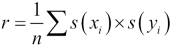
In this case, is the standardized score for each individual value, . We do the same calculation for the other sequences and compute the product of each pair. The average of the product of the various standardized scores will be a value between +1 and -1. A value near +1 means the two sequences correlate nicely. A value near -1 means the sequences oppose each other. One trends up when the other trends down. A value near 0 means the sequences don't correlate.

Here's a function that computes the correlation between two instances of AnnualStat data collections:

def correlation1( d1, d2 ):
    n= len(d1.data)
    std_score_pairs = zip( d1.stdscore(), d2.stdscore() )
    r = sum( x*y for x,y in std_score_pairs )/n
    return r

We used the stdscore() method of each AnnualStat object to create a sequence of standardized score values.

We created a generator using the zip() function that will yield two-tuples from two separate sequences of scores. The mean of this sequence of products is the coefficient correlation between the two sequences. We computed the mean by summing and dividing by the length, n.