Table of Contents for
R Cookbook, 2nd Edition
 R Cookbook, 2nd Edition
Published by
O'Reilly Media, Inc., 2019
R Cookbook, 2nd Edition
Published by
O'Reilly Media, Inc., 2019
Chapter 8. Probability
Introduction
Probability theory is the foundation of statistics, and R has plenty of machinery for working with probability, probability distributions, and random variables. The recipes in this chapter show you how to calculate probabilities from quantiles, calculate quantiles from probabilities, generate random variables drawn from distributions, plot distributions, and so forth.
Names of Distributions
R has an abbreviated name for every probability distribution. This name is used to identify the functions associated with the distribution. For example, the name of the Normal distribution is “norm”, which is the root of these function names:
| Function | Purpose |
|---|---|
|
Normal density |
|
Normal distribution function |
|
Normal quantile function |
|
Normal random variates |
Table 8-1 describes some common discrete distributions, and Table 8-2 describes several common continuous distributions.
| Discrete distribution | R name | Parameters |
|---|---|---|
Binomial |
binom |
n = number of trials; p = probability of success for one trial |
Geometric |
geom |
p = probability of success for one trial |
Hypergeometric |
hyper |
m = number of white balls in urn; n = number of black balls in urn; k = number of balls drawn from urn |
Negative binomial (NegBinomial) |
nbinom |
size = number of successful trials; either prob = probability of successful trial or mu = mean |
Poisson |
pois |
lambda = mean |
| Continuous distribution | R name | Parameters |
|---|---|---|
Beta |
beta |
shape1; shape2 |
Cauchy |
cauchy |
location; scale |
Chi-squared (Chisquare) |
chisq |
df = degrees of freedom |
Exponential |
exp |
rate |
F |
f |
df1 and df2 = degrees of freedom |
Gamma |
gamma |
rate; either rate or scale |
Log-normal (Lognormal) |
lnorm |
meanlog = mean on logarithmic scale; |
sdlog = standard deviation on logarithmic scale |
||
Logistic |
logis |
location; scale |
Normal |
norm |
mean; sd = standard deviation |
Student’s t (TDist) |
t |
df = degrees of freedom |
Uniform |
unif |
min = lower limit; max = upper limit |
Weibull |
weibull |
shape; scale |
Wilcoxon |
wilcox |
m = number of observations in first sample; |
n = number of observations in second sample |
Warning
All distribution-related functions require distributional parameters,
such as size and prob for the binomial or prob for the geometric.
The big “gotcha” is that the distributional parameters may not be what
you expect. For example, I would expect the parameter of an exponential
distribution to be β, the mean. The R convention, however, is for the
exponential distribution to be defined by the rate = 1/β, so I often
supply the wrong value. The moral is, study the help page before you use
a function related to a distribution. Be sure you’ve got the parameters
right.
Getting Help on Probability Distributions
To see the R functions related to a particular probability distribution, use the help command and the full name of the distribution. For example, this will show the functions related to the Normal distribution:
?Normal
Some distributions have names that don’t work well with the help command, such as “Student’s t”. They have special help names, as noted in Tables Table 8-1 and Table 8-2: NegBinomial, Chisquare, Lognormal, and TDist. Thus, to get help on the Student’s t distribution, use this:
?TDist
See Also
There are many other distributions implemented in downloadable packages;
see the CRAN task view devoted to
probability
distributions. The SuppDists package is part of the R base, and it
includes ten supplemental distributions. The MASS package, which is
also part of the base, provides additional support for distributions,
such as maximum-likelihood fitting for some common distributions as well
as sampling from a multivariate Normal distribution.
Counting the Number of Combinations
Problem
You want to calculate the number of combinations of n items taken k at a time.
Solution
Use the choose function:
n<-10k<-2choose(n,k)#> [1] 45
Discussion
A common problem in computing probabilities of discrete variables is
counting combinations: the number of distinct subsets of size k that
can be created from n items. The number is given by n!/r!(n −
r)!, but it’s much more convenient to use the choose
function—especially as n and k grow larger:
choose(5,3)# How many ways can we select 3 items from 5 items?#> [1] 10choose(50,3)# How many ways can we select 3 items from 50 items?#> [1] 19600choose(50,30)# How many ways can we select 30 items from 50 items?#> [1] 4.71e+13
These numbers are also known as binomial coefficients.
See Also
This recipe merely counts the combinations; see “Generating Combinations” to actually generate them.
Generating Combinations
Problem
You want to generate all combinations of n items taken k at a time.
Solution
Use the combn function:
items<-2:5k<-2combn(items,k)#> [,1] [,2] [,3] [,4] [,5] [,6]#> [1,] 2 2 2 3 3 4#> [2,] 3 4 5 4 5 5
Discussion
We can use combn(1:5,3) to generate all combinations of the numbers 1
through 5 taken three at a time:
combn(1:5,3)#> [,1] [,2] [,3] [,4] [,5] [,6] [,7] [,8] [,9] [,10]#> [1,] 1 1 1 1 1 1 2 2 2 3#> [2,] 2 2 2 3 3 4 3 3 4 4#> [3,] 3 4 5 4 5 5 4 5 5 5
The function is not restricted to numbers. We can generate combinations of strings, too. Here are all combinations of five treatments taken three at a time:
combn(c("T1","T2","T3","T4","T5"),3)#> [,1] [,2] [,3] [,4] [,5] [,6] [,7] [,8] [,9] [,10]#> [1,] "T1" "T1" "T1" "T1" "T1" "T1" "T2" "T2" "T2" "T3"#> [2,] "T2" "T2" "T2" "T3" "T3" "T4" "T3" "T3" "T4" "T4"#> [3,] "T3" "T4" "T5" "T4" "T5" "T5" "T4" "T5" "T5" "T5"
Warning
As the number of items, n, increases, the number of combinations can explode—especially if k is not near to 1 or n.
See Also
See “Counting the Number of Combinations” to count the number of possible combinations before you generate a huge set.
Generating Random Numbers
Problem
You want to generate random numbers.
Solution
The simple case of generating a uniform random number between 0 and 1 is
handled by the runif function. This example generates one uniform
random number:
runif(1)#> [1] 0.915
Note
If you are saying runif out loud (or even in your head), you
should pronounce it “are unif” instead of “run if.” The term runif is
a portmanteau of “random uniform” so should not sound as if it’s a
flow control function.
R can generate random variates from other distributions as well. For a
given distribution, the name of the random number generator is “r”
prefixed to the distribution’s abbreviated name (e.g., rnorm for the
Normal distribution’s random number generator). This example generates
one random value from the standard normal distribution:
rnorm(1)#> [1] 1.53
Discussion
Most programming languages have a wimpy random number generator that generates one random number, uniformly distributed between 0.0 and 1.0, and that’s all. Not R.
R can generate random numbers from many probability distributions other
than the uniform distribution. The simple case of generating uniform
random numbers between 0 and 1 is handled by the runif function:
runif(1)#> [1] 0.83
The argument of runif is the number of random values to be generated.
Generating a vector of 10 such values is as easy as generating one:
runif(10)#> [1] 0.642 0.519 0.737 0.135 0.657 0.705 0.458 0.719 0.935 0.255
There are random number generators for all built-in distributions. Simply prefix the distribution name with “r” and you have the name of the corresponding random number generator. Here are some common ones:
set.seed(42)runif(1,min=-3,max=3)# One uniform variate between -3 and +3#> [1] 2.49rnorm(1)# One standard Normal variate#> [1] 1.53rnorm(1,mean=100,sd=15)# One Normal variate, mean 100 and SD 15#> [1] 114rbinom(1,size=10,prob=0.5)# One binomial variate#> [1] 5rpois(1,lambda=10)# One Poisson variate#> [1] 12rexp(1,rate=0.1)# One exponential variate#> [1] 3.14rgamma(1,shape=2,rate=0.1)# One gamma variate#> [1] 22.3
As with runif, the first argument is the number of random values to be
generated. Subsequent arguments are the parameters of the distribution,
such as mean and sd for the Normal distribution or size and prob
for the binomial. See the function’s R help page for details.
The examples given so far use simple scalars for distributional parameters. Yet the parameters can also be vectors, in which case R will cycle through the vector while generating random values. The following example generates three normal random values drawn from distributions with means of −10, 0, and +10, respectively (all distributions have a standard deviation of 1.0):
rnorm(3,mean=c(-10,0,+10),sd=1)#> [1] -9.420 -0.658 11.555
That is a powerful capability in such cases as hierarchical models, where the parameters are themselves random. The next example calculates 30 draws of a normal variate whose mean is itself randomly distributed and with hyperparameters of μ = 0 and σ = 0.2:
means<-rnorm(30,mean=0,sd=0.2)rnorm(30,mean=means,sd=1)#> [1] -0.5549 -2.9232 -1.2203 0.6962 0.1673 -1.0779 -0.3138 -3.3165#> [9] 1.5952 0.8184 -0.1251 0.3601 -0.8142 0.1050 2.1264 0.6943#> [17] -2.7771 0.9026 0.0389 0.2280 -0.5599 0.9572 0.1972 0.2602#> [25] -0.4423 1.9707 0.4553 0.0467 1.5229 0.3176
If you are generating many random values and the vector of parameters is too short, R will apply the Recycling Rule to the parameter vector.
See Also
See the “Introduction” to this chapter.
Generating Reproducible Random Numbers
Problem
You want to generate a sequence of random numbers, but you want to reproduce the same sequence every time your program runs.
Solution
Before running your R code, call the set.seed function to initialize
the random number generator to a known state:
set.seed(42)# Or use any other positive integer...
Discussion
After generating random numbers, you may often want to reproduce the same sequence of “random” numbers every time your program executes. That way, you get the same results from run to run. One of the authors (Paul) once supported a complicated Monte Carlo analysis of a huge portfolio of securities. The users complained about getting slightly different results each time the program ran. No kidding! The analysis was driven entirely by random numbers, so of course there was randomness in the output. The solution was to set the random number generator to a known state at the beginning of the program. That way, it would generate the same (quasi-)random numbers each time and thus yield consistent, reproducible results.
In R, the set.seed function sets the random number generator to a
known state. The function takes one argument, an integer. Any positive
integer will work, but you must use the same one in order to get the
same initial state.
The function returns nothing. It works behind the scenes, initializing (or reinitializing) the random number generator. The key here is that using the same seed restarts the random number generator back at the same place:
set.seed(165)# Initialize generator to known staterunif(10)# Generate ten random numbers#> [1] 0.116 0.450 0.996 0.611 0.616 0.426 0.666 0.168 0.788 0.442set.seed(165)# Reinitialize to the same known staterunif(10)# Generate the same ten "random" numbers#> [1] 0.116 0.450 0.996 0.611 0.616 0.426 0.666 0.168 0.788 0.442
Warning
When you set the seed value and freeze your sequence of random numbers,
you are eliminating a source of randomness that may be critical to
algorithms such as Monte Carlo simulations. Before you call set.seed
in your application, ask yourself: Am I undercutting the value of my
program or perhaps even damaging its logic?
See Also
See “Generating Random Numbers” for more about generating random numbers.
Generating a Random Sample
Problem
You want to sample a dataset randomly.
Solution
The sample function will randomly select n items from a set:
sample(set,n)
Discussion
Suppose your World Series data contains a vector of years when the
Series was played. You can select 10 years at random using sample:
world_series<-read_csv("./data/world_series.csv")sample(world_series$year,10)#> [1] 2010 1961 1906 1992 1982 1948 1910 1973 1967 1931
The items are randomly selected, so running sample again (usually)
produces a different result:
sample(world_series$year,10)#> [1] 1941 1973 1921 1958 1979 1946 1932 1919 1971 1974
The sample function normally samples without replacement, meaning it
will not select the same item twice. Some statistical procedures
(especially the bootstrap) require sampling with replacement, which
means that one item can appear multiple times in the sample. Specify
replace=TRUE to sample with replacement.
It’s easy to implement a simple bootstrap using sampling with
replacement. Suppose we have a vector, x, of 1,000 random numbers,
drawn from a normal distribution with mean 4 and standard deviation 10.
set.seed(42)x<-rnorm(1000,4,10)
This code fragment samples 1,000 times from x and calculates the
median of each sample:
medians<-numeric(1000)# empty vector of 1000 numbersfor(iin1:1000){medians[i]<-median(sample(x,replace=TRUE))}
From the bootstrap estimates, we can estimate the confidence interval for the median:
ci<-quantile(medians,c(0.025,0.975))cat("95% confidence interval is (",ci,")\n")#> 95% confidence interval is ( 3.16 4.49 )
We know that x was created from a normal distribution with a mean of 4
and, hence, the sample median should be 4 also. (In a symetrical
distribution like the normal, the mean and the median are the same.) Our
confidence interval easily contains the value.
See Also
See “Randomly Permuting a Vector” for randomly permuting a vector and Recipe X-X for more about bootstrapping. “Generating Reproducible Random Numbers” discusses setting seeds for quasi-random numbers.
Generating Random Sequences
Problem
You want to generate a random sequence, such as a series of simulated coin tosses or a simulated sequence of Bernoulli trials.
Solution
Use the sample function. Sample n draws from the set of possible
values, and set replace=TRUE:
sample(set,n,replace=TRUE)
Discussion
The sample function randomly selects items from a set. It normally
samples without replacement, which means that it will not select the
same item twice and will return an error if you try to sample more items
than exist in the set. With replace=TRUE, however, sample can select
items over and over; this allows you to generate long, random sequences
of items.
The following example generates a random sequence of 10 simulated flips of a coin:
sample(c("H","T"),10,replace=TRUE)#> [1] "H" "T" "H" "T" "T" "T" "H" "T" "T" "H"
The next example generates a sequence of 20 Bernoulli trials—random
successes or failures. We use TRUE to signify a success:
sample(c(FALSE,TRUE),20,replace=TRUE)#> [1] TRUE FALSE TRUE TRUE FALSE TRUE FALSE FALSE TRUE TRUE FALSE#> [12] TRUE TRUE FALSE TRUE TRUE FALSE FALSE FALSE FALSE
By default, sample will choose equally among the set elements and so
the probability of selecting either TRUE or FALSE is 0.5. With a
Bernoulli trial, the probability p of success is not necessarily 0.5.
You can bias the sample by using the prob argument of sample; this
argument is a vector of probabilities, one for each set element. Suppose
we want to generate 20 Bernoulli trials with a probability of success
p = 0.8. We set the probability of FALSE to be 0.2 and the
probability of TRUE to 0.8:
sample(c(FALSE,TRUE),20,replace=TRUE,prob=c(0.2,0.8))#> [1] TRUE TRUE FALSE TRUE TRUE TRUE TRUE TRUE TRUE TRUE TRUE#> [12] TRUE TRUE TRUE TRUE TRUE FALSE FALSE TRUE TRUE
The resulting sequence is clearly biased toward TRUE. I chose this
example because it’s a simple demonstration of a general technique. For
the special case of a binary-valued sequence you can use rbinom, the
random generator for binomial variates:
rbinom(10,1,0.8)#> [1] 1 0 1 1 1 1 1 0 1 1
Randomly Permuting a Vector
Problem
You want to generate a random permutation of a vector.
Solution
If v is your vector, then sample(v) returns a random permutation.
Discussion
We typically think of the sample function for sampling from large
datasets. However, the default parameters enable you to create a random
rearrangement of the dataset. The function call sample(v) is
equivalent to:
sample(v,size=length(v),replace=FALSE)
which means “select all the elements of v in random order while using
each element exactly once.” That is a random permutation. Here is a
random permutation of 1, …, 10:
sample(1:10)#> [1] 7 3 6 1 5 2 4 8 10 9
See Also
See “Generating a Random Sample” for more about sample.
Calculating Probabilities for Discrete Distributions
Problem
You want to calculate either the simple or the cumulative probability associated with a discrete random variable.
Solution
For a simple probability, P(X = x), use the density function. All
built-in probability distributions have a density function whose name is
“d” prefixed to the distribution name. For example, dbinom for the
binomial distribution.
For a cumulative probability, P(X ≤ x), use the distribution
function. All built-in probability distributions have a distribution
function whose name is “p” prefixed to the distribution name; thus,
pbinom is the distribution function for the binomial distribution.
Discussion
Suppose we have a binomial random variable X over 10 trials, where
each trial has a success probability of 1/2. Then we can calculate the
probability of observing x = 7 by calling dbinom:
dbinom(7,size=10,prob=0.5)#> [1] 0.117
That calculates a probability of about 0.117. R calls dbinom the
density function. Some textbooks call it the probability mass function
or the probability function. Calling it a density function keeps the
terminology consistent between discrete and continuous distributions
(“Calculating Probabilities for Continuous Distributions”).
The cumulative probability, P(X ≤ x), is given by the distribution
function, which is sometimes called the cumulative probability function.
The distribution function for the binomial distribution is pbinom.
Here is the cumulative probability for x = 7 (i.e., P(X ≤ 7)):
pbinom(7,size=10,prob=0.5)#> [1] 0.945
It appears the probability of observing X ≤ 7 is about 0.945.
The density functions and distribution functions for some common discrete distributions are shown in Table @ref(tab:distributions).
| Distribution | Density function: P(X = x) | Distribution function: P(X ≤ x) |
|---|---|---|
Binomial |
dbinom(x, size, prob) |
pbinom(x, size, prob) |
Geometric |
dgeom(x, prob) |
pgeom(x, prob) |
Poisson |
dpois(x, lambda) |
ppois(x, lambda) |
The complement of the cumulative probability is the survival function,
P(X > x). All of the distribution functions let you find this
right-tail probability simply by specifying lower.tail=FALSE:
pbinom(7,size=10,prob=0.5,lower.tail=FALSE)#> [1] 0.0547
Thus we see that the probability of observing X > 7 is about 0.055.
The interval probability, P(x1 < X ≤ x2), is the probability of observing X between the limits x1 and x2. It is calculated as the difference between two cumulative probabilities: P(X ≤ x2) − P(X ≤ x1). Here is P(3 < X ≤ 7) for our binomial variable:
pbinom(7,size=10,prob=0.5)-pbinom(3,size=10,prob=0.5)#> [1] 0.773
R lets you specify multiple values of x for these functions and will
return a vector of the corresponding probabilities. Here we calculate
two cumulative probabilities, P(X ≤ 3) and P(X ≤ 7), in one call
to pbinom:
pbinom(c(3,7),size=10,prob=0.5)#> [1] 0.172 0.945
This leads to a one-liner for calculating interval probabilities. The
diff function calculates the difference between successive elements of
a vector. We apply it to the output of pbinom to obtain the difference
in cumulative probabilities—in other words, the interval probability:
diff(pbinom(c(3,7),size=10,prob=0.5))#> [1] 0.773
See Also
See this chapter’s “Introduction” for more about the built-in probability distributions.
Calculating Probabilities for Continuous Distributions
Problem
You want to calculate the distribution function (DF) or cumulative distribution function (CDF) for a continuous random variable.
Solution
Use the distribution function, which calculates P(X ≤ x). All
built-in probability distributions have a distribution function whose
name is “p” prefixed to the distribution’s abbreviated name—for
instance, pnorm for the Normal distribution.
Example: what’s the probability of a draw being below .8 for a draw from a random standard normal distribution?
pnorm(q=.8,mean=0,sd=1)#> [1] 0.788
Discussion
The R functions for probability distributions follow a consistent pattern, so the solution to this recipe is essentially identical to the solution for discrete random variables (“Calculating Probabilities for Discrete Distributions”). The significant difference is that continuous variables have no “probability” at a single point, P(X = x). Instead, they have a density at a point.
Given that consistency, the discussion of distribution functions in “Calculating Probabilities for Discrete Distributions” is applicable here, too. Table @ref(tab:continuous) gives the distribution functions for several continuous distributions.
| Distribution | Distribution function: P(X ≤ x) |
|---|---|
Normal |
pnorm(x, mean, sd) |
Student’s t |
pt(x, df) |
Exponential |
pexp(x, rate) |
Gamma |
pgamma(x, shape, rate) |
Chi-squared (χ2) |
pchisq(x, df) |
We can use pnorm to calculate the probability that a man is shorter
than 66 inches, assuming that men’s heights are normally distributed
with a mean of 70 inches and a standard deviation of 3 inches.
Mathematically speaking, we want P(X ≤ 66) given that X ~ N(70,
3):
pnorm(66,mean=70,sd=3)#> [1] 0.0912
Likewise, we can use pexp to calculate the probability that an
exponential variable with a mean of 40 could be less than 20:
pexp(20,rate=1/40)#> [1] 0.393
Just as for discrete probabilities, the functions for continuous
probabilities use lower.tail=FALSE to specify the survival function,
P(X > x). This call to pexp gives the probability that the same
exponential variable could be greater than 50:
pexp(50,rate=1/40,lower.tail=FALSE)#> [1] 0.287
Also like discrete probabilities, the interval probability for a continuous variable, P(x1 < X < x2), is computed as the difference between two cumulative probabilities, P(X < x2) − P(X < x1). For the same exponential variable, here is P(20 < X < 50), the probability that it could fall between 20 and 50:
pexp(50,rate=1/40)-pexp(20,rate=1/40)#> [1] 0.32
See Also
See this chapter’s “Introduction” for more about the built-in probability distributions.
Converting Probabilities to Quantiles
Problem
Given a probability p and a distribution, you want to determine the corresponding quantile for p: the value x such that P(X ≤ x) = p.
Solution
Every built-in distribution includes a quantile function that converts
probabilities to quantiles. The function’s name is “q” prefixed to the
distribution name; thus, for instance, qnorm is the quantile function
for the Normal distribution.
The first argument of the quantile function is the probability. The remaining arguments are the distribution’s parameters, such as mean, shape, or rate:
qnorm(0.05,mean=100,sd=15)#> [1] 75.3
Discussion
A common example of computing quantiles is when we compute the limits of a confidence interval. If we want to know the 95% confidence interval (α = 0.05) of a standard normal variable, then we need the quantiles with probabilities of α/2 = 0.025 and (1 − α)/2 = 0.975:
qnorm(0.025)#> [1] -1.96qnorm(0.975)#> [1] 1.96
In the true spirit of R, the first argument of the quantile functions can be a vector of probabilities, in which case we get a vector of quantiles. We can simplify this example into a one-liner:
qnorm(c(0.025,0.975))#> [1] -1.96 1.96
All the built-in probability distributions provide a quantile function. Table @ref(tab:discrete-quant-dist) shows the quantile functions for some common discrete distributions.
| Distribution | Quantile function |
|---|---|
Binomial |
qbinom(p, size, prob) |
Geometric |
qgeom(p, prob) |
Poisson |
qpois(p, lambda) |
Table @ref(tab:cont-quant-dist) shows the quantile functions for common continuous distributions.
| Distribution | Quantile function |
|---|---|
Normal |
qnorm(p, mean, sd) |
Student’s t |
qt(p, df) |
Exponential |
qexp(p, rate) |
Gamma |
qgamma(p, shape, rate=rate) or qgamma(p, shape, scale=scale) |
Chi-squared (χ2) |
qchisq(p, df) |
See Also
Determining the quantiles of a data set is different from determining the quantiles of a distribution—see “Calculating Quantiles (and Quartiles) of a Dataset”.
Plotting a Density Function
Problem
You want to plot the density function of a probability distribution.
Solution
Define a vector x over the domain. Apply the distribution’s density
function to x and then plot the result. If x is a vector of points
over the domain we care about plotting, we then calculate the density
using one of the d_____ density functions like dlnorm for lognormal
or dnorm for normal.
dens<-data.frame(x=x,y=d_____(x))ggplot(dens,aes(x,y))+geom_line()
Here is a specific example that plots the standard normal distribution for the interval -3 to +3:
library(ggplot2)x<-seq(-3,+3,0.1)dens<-data.frame(x=x,y=dnorm(x))ggplot(dens,aes(x,y))+geom_line()
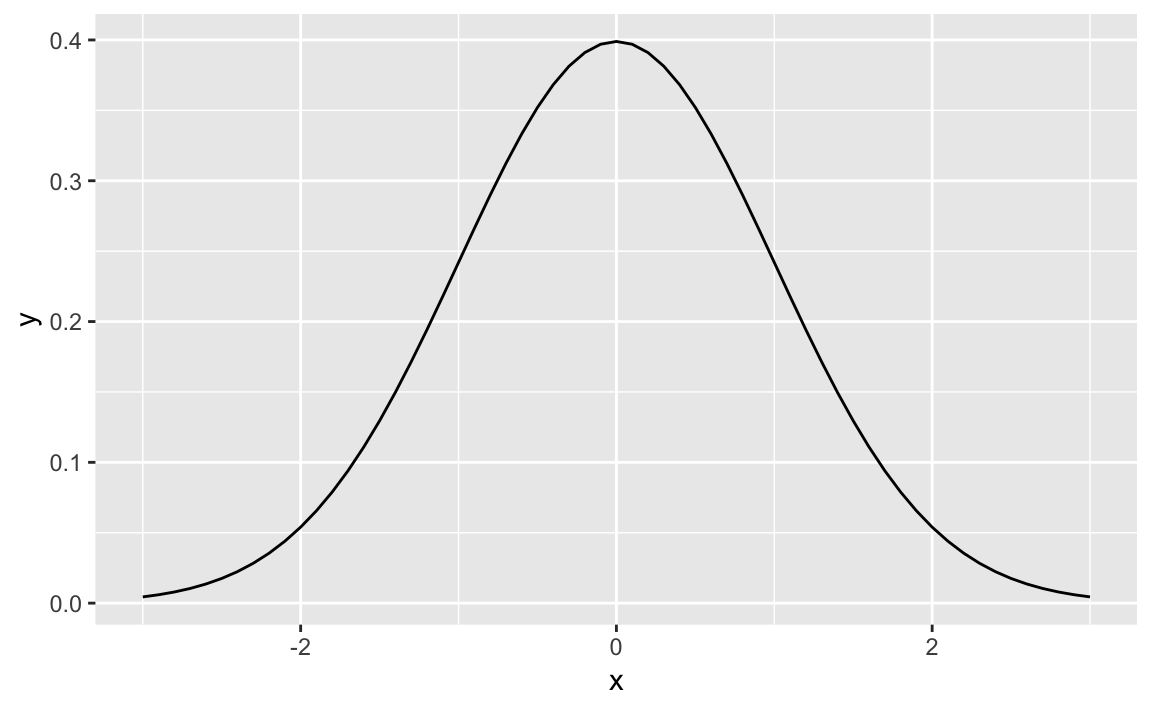
Figure 8-1. Standard Normal
Figure 8-1 shows the smooth density function.
Discussion
All the built-in probability distributions include a density function.
For a particular density, the function name is “d” prepended to the
density name. The density function for the Normal distribution is
dnorm, the density for the gamma distribution is dgamma, and so
forth.
If the first argument of the density function is a vector, then the function calculates the density at each point and returns the vector of densities.
The following code creates a 2 × 2 plot of four densities:
x<-seq(from=0,to=6,length.out=100)# Define the density domainsylim<-c(0,0.6)# Make a data.frame with densities of several distributionsdf<-rbind(data.frame(x=x,dist_name="Uniform",y=dunif(x,min=2,max=4)),data.frame(x=x,dist_name="Normal",y=dnorm(x,mean=3,sd=1)),data.frame(x=x,dist_name="Exponential",y=dexp(x,rate=1/2)),data.frame(x=x,dist_name="Gamma",y=dgamma(x,shape=2,rate=1)))# Make a line plot like before, but use facet_wrap to create the gridggplot(data=df,aes(x=x,y=y))+geom_line()+facet_wrap(~dist_name)# facet and wrap by the variable dist_name
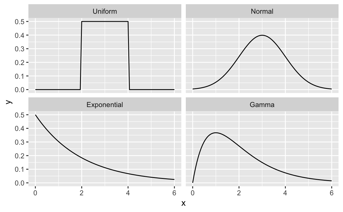
Figure 8-2. Multiple Density Plots
Figure 8-2 shows four density plots. However, a raw density plot is rarely useful or interesting by itself, and we often shade a region of interest.
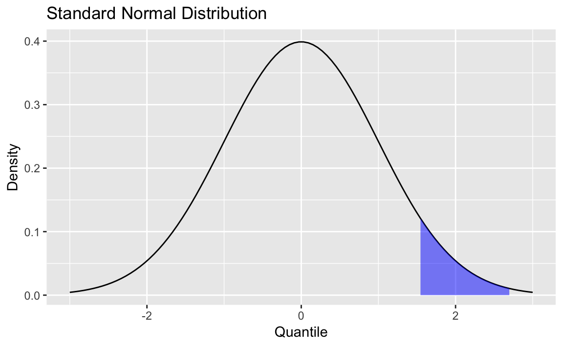
Figure 8-3. Standard Normal with Shading
Figure 8-3 is a normal distribution with shading from the 75th percentile to the 95th percentile.
We create the plot by first plotting the density and then creating a
shaded region with the geom_ribbon function from ggplot2.
First, we create some data and draw the density curve shown in Figure 8-4
x<-seq(from=-3,to=3,length.out=100)df<-data.frame(x=x,y=dnorm(x,mean=0,sd=1))p<-ggplot(df,aes(x,y))+geom_line()+labs(title="Standard Normal Distribution",y="Density",x="Quantile")p
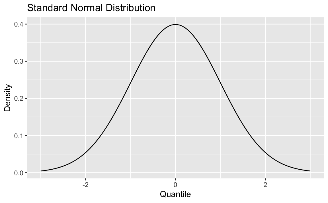
Figure 8-4. Density Plot
Next, we define the region of interest by calculating the x value for
the quantiles we’re interested in. Then finally we add a geom_ribbon
to add a subset of our original data as a colored region. The resulting
plot is shown here:
q75<-quantile(df$x,.75)q95<-quantile(df$x,.95)p+geom_ribbon(data=subset(df,x>q75&x<q95),aes(ymax=y),ymin=0,fill="blue",colour=NA,alpha=0.5)