Table of Contents for
R Cookbook, 2nd Edition
 R Cookbook, 2nd Edition
Published by
O'Reilly Media, Inc., 2019
R Cookbook, 2nd Edition
Published by
O'Reilly Media, Inc., 2019
Chapter 4. Input and Output
***todo: add base R options at end of tidy recipes?
Introduction
All statistical work begins with data, and most data is stuck inside files and databases. Dealing with input is probably the first step of implementing any significant statistical project.
All statistical work ends with reporting numbers back to a client, even if you are the client. Formatting and producing output is probably the climax of your project.
Casual R users can solve their input problems by using basic functions
such as read.csv to read CSV files and read.table to read more
complicated, tabular data. They can use print, cat, and format to
produce simple reports.
Users with heavy-duty input/output (I/O) needs are strongly encouraged to read the R Data Import/Export guide, available on CRAN at http://cran.r-project.org/doc/manuals/R-data.pdf. This manual includes important information on reading data from sources such as spreadsheets, binary files, other statistical systems, and relational databases.
Entering Data from the Keyboard
Problem
You have a small amount of data, too small to justify the overhead of creating an input file. You just want to enter the data directly into your workspace.
Solution
For very small datasets, enter the data as literals using the c()
constructor for vectors:
scores<-c(61,66,90,88,100)
Discussion
When working on a simple problem, you may not want the hassle of
creating and then reading a data file outside of R. You may just want to
enter the data into R. The easiest way is by using the c() constructor
for vectors, as shown in the Solution.
This approach works for data frames, too, by entering each variable (column) as a vector:
points<-data.frame(label=c("Low","Mid","High"),lbound=c(0,0.67,1.64),ubound=c(0.67,1.64,2.33))
See Also
See Recipe X-X for more about using the built-in data editor, as suggested in the Solution.
For cutting and pasting data from another application into R, be sure
and look at datapasta, a package that provides R Studio addins that
make pasting data into your scripts easier:
https://github.com/MilesMcBain/datapasta
Printing Fewer Digits (or More Digits)
Problem
Your output contains too many digits or too few digits. You want to print fewer or more.
Solution
For print, the digits parameter can control the number of printed
digits.
For cat, use the format function (which also has a digits
parameter) to alter the formatting of numbers.
Discussion
R normally formats floating-point output to have seven digits:
pi#> [1] 3.14100*pi#> [1] 314
This works well most of the time but can become annoying when you have lots of numbers to print in a small space. It gets downright misleading when there are only a few significant digits in your numbers and R still prints seven.
The print function lets you vary the number of printed digits using
the digits parameter:
(pi,digits=4)#> [1] 3.142(100*pi,digits=4)#> [1] 314.2
The cat function does not give you direct control over formatting.
Instead, use the format function to format your numbers before calling
cat:
cat(pi,"\n")#> 3.14cat(format(pi,digits=4),"\n")#> 3.142
This is R, so both print and format will format entire vectors at
once:
pnorm(-3:3)#> [1] 0.00135 0.02275 0.15866 0.50000 0.84134 0.97725 0.99865(pnorm(-3:3),digits=3)#> [1] 0.00135 0.02275 0.15866 0.50000 0.84134 0.97725 0.99865
Notice that print formats the vector elements consistently: finding
the number of digits necessary to format the smallest number and then
formatting all numbers to have the same width (though not necessarily
the same number of digits). This is extremely useful for formating an
entire table:
q<-seq(from=0,to=3,by=0.5)tbl<-data.frame(Quant=q,Lower=pnorm(-q),Upper=pnorm(q))tbl# Unformatted print#> Quant Lower Upper#> 1 0.0 0.50000 0.500#> 2 0.5 0.30854 0.691#> 3 1.0 0.15866 0.841#> 4 1.5 0.06681 0.933#> 5 2.0 0.02275 0.977#> 6 2.5 0.00621 0.994#> 7 3.0 0.00135 0.999(tbl,digits=2)# Formatted print: fewer digits#> Quant Lower Upper#> 1 0.0 0.5000 0.50#> 2 0.5 0.3085 0.69#> 3 1.0 0.1587 0.84#> 4 1.5 0.0668 0.93#> 5 2.0 0.0228 0.98#> 6 2.5 0.0062 0.99#> 7 3.0 0.0013 1.00
You can also alter the format of all output by using the options
function to change the default for digits:
pi#> [1] 3.14options(digits=15)pi#> [1] 3.14159265358979
But this is a poor choice in our experience, since it also alters the output from R’s built-in functions, and that alteration may likely be unpleasant.
See Also
Other functions for formatting numbers include sprintf and formatC;
see their help pages for details.
Redirecting Output to a File
Problem
You want to redirect the output from R into a file instead of your console.
Solution
You can redirect the output of the cat function by using its file
argument:
cat("The answer is",answer,"\n",file="filename.txt")
Use the sink function to redirect all output from both print and
cat. Call sink with a filename argument to begin redirecting console
output to that file. When you are done, use sink with no argument to
close the file and resume output to the console:
sink("filename")# Begin writing output to file# ... other session work ...sink()# Resume writing output to console
Discussion
The print and cat functions normally write their output to your
console. The cat function writes to a file if you supply a file
argument, which can be either a filename or a connection. The print
function cannot redirect its output, but the sink function can force all
output to a file. A common use for sink is to capture the output of an R
script:
sink("script_output.txt")# Redirect output to filesource("script.R")# Run the script, capturing its outputsink()# Resume writing output to console
If you are repeatedly cat`ing items to one file, be sure to set
`append=TRUE. Otherwise, each call to cat will simply overwrite the
file’s contents:
cat(data,file="analysisReport.out")cat(results,file="analysisRepart.out",append=TRUE)cat(conclusion,file="analysisReport.out",append=TRUE)
Hard-coding file names like this is a tedious and error-prone process. Did you notice that the filename is misspelled in the second line? Instead of hard-coding the filename repeatedly, I suggest opening a connection to the file and writing your output to the connection:
con<-file("analysisReport.out","w")cat(data,file=con)cat(results,file=con)cat(conclusion,file=con)close(con)
(You don’t need append=TRUE when writing to a connection because
append is the default with connections.) This technique is especially
valuable inside R scripts because it makes your code more reliable and
more maintainable.
Listing Files
Problem
You want an R vector that is a listing of the files in your working directory.
Solution
The list.files function shows the contents of your working directory:
list.files()#> [1] "_book" "_bookdown_files"#> [3] "_bookdown_files.old" "_bookdown.yml"#> [5] "_common.R" "_main.rds"#> [7] "_output.yaml" "01_GettingStarted_cache"#> [9] "01_GettingStarted.md" "01_GettingStarted.Rmd"etc...
Discussion
This function is terribly handy to grab the names of all files in a subdirectory. You can use it to refresh your memory of your file names or, more likely, as input into another process, like importing data files.
You can pass list.files a path and a pattern to shows files in a
specific path and matching a specific regular expression pattern.
list.files(path='data/')# show files in a directory#> [1] "ac.rdata" "adf.rdata"#> [3] "anova.rdata" "anova2.rdata"#> [5] "bad.rdata" "batches.rdata"#> [7] "bnd_cmty.Rdata" "compositePerf-2010.csv"#> [9] "conf.rdata" "daily.prod.rdata"#> [11] "data1.csv" "data2.csv"#> [13] "datafile_missing.tsv" "datafile.csv"#> [15] "datafile.fwf" "datafile.qsv"#> [17] "datafile.ssv" "datafile.tsv"#> [19] "df_decay.rdata" "df_squared.rdata"#> [21] "diffs.rdata" "example1_headless.csv"#> [23] "example1.csv" "excel_table_data.xlsx"#> [25] "get_USDA_NASS_data.R" "ibm.rdata"#> [27] "iris_excel.xlsx" "lab_df.rdata"#> [29] "movies.sas7bdat" "nacho_data.csv"#> [31] "NearestPoint.R" "not_a_csv.txt"#> [33] "opt.rdata" "outcome.rdata"#> [35] "pca.rdata" "pred.rdata"#> [37] "pred2.rdata" "sat.rdata"#> [39] "singles.txt" "state_corn_yield.rds"#> [41] "student_data.rdata" "suburbs.txt"#> [43] "tab1.csv" "tls.rdata"#> [45] "triples.txt" "ts_acf.rdata"#> [47] "workers.rdata" "world_series.csv"#> [49] "xy.rdata" "yield.Rdata"#> [51] "z.RData"list.files(path='data/',pattern='\\.csv')#> [1] "compositePerf-2010.csv" "data1.csv"#> [3] "data2.csv" "datafile.csv"#> [5] "example1_headless.csv" "example1.csv"#> [7] "nacho_data.csv" "tab1.csv"#> [9] "world_series.csv"
To see all the files in your subdirectories, too, use
list.files(recursive=T)
A possible “gotcha” of list.files is that it ignores hidden
files—typically, any file whose name begins with a period. If you don’t
see the file you expected to see, try setting all.files=TRUE:
list.files(path='data/',all.files=TRUE)#> [1] "." ".."#> [3] ".DS_Store" ".hidden_file.txt"#> [5] "ac.rdata" "adf.rdata"#> [7] "anova.rdata" "anova2.rdata"#> [9] "bad.rdata" "batches.rdata"#> [11] "bnd_cmty.Rdata" "compositePerf-2010.csv"#> [13] "conf.rdata" "daily.prod.rdata"#> [15] "data1.csv" "data2.csv"#> [17] "datafile_missing.tsv" "datafile.csv"#> [19] "datafile.fwf" "datafile.qsv"#> [21] "datafile.ssv" "datafile.tsv"#> [23] "df_decay.rdata" "df_squared.rdata"#> [25] "diffs.rdata" "example1_headless.csv"#> [27] "example1.csv" "excel_table_data.xlsx"#> [29] "get_USDA_NASS_data.R" "ibm.rdata"#> [31] "iris_excel.xlsx" "lab_df.rdata"#> [33] "movies.sas7bdat" "nacho_data.csv"#> [35] "NearestPoint.R" "not_a_csv.txt"#> [37] "opt.rdata" "outcome.rdata"#> [39] "pca.rdata" "pred.rdata"#> [41] "pred2.rdata" "sat.rdata"#> [43] "singles.txt" "state_corn_yield.rds"#> [45] "student_data.rdata" "suburbs.txt"#> [47] "tab1.csv" "tls.rdata"#> [49] "triples.txt" "ts_acf.rdata"#> [51] "workers.rdata" "world_series.csv"#> [53] "xy.rdata" "yield.Rdata"#> [55] "z.RData"
If you just want to see which files are in a directory and not use the
file names in a procedure, the easiest way is to open the Files pane
in the lower right corner of RStudio. But keep in mind that the RStudio
Files pane hides files that start with a . as you can see in ???:
. image::images_v2/rstudio.files2.png[]
See Also
R has other handy functions for working with files; see help(files).
Dealing with “Cannot Open File” in Windows
Problem
You are running R on Windows, and you are using file names such as
C:\data\sample.txt. R says it cannot open the file, but you know the
file does exist.
Solution
The backslashes in the file path are causing trouble. You can solve this problem in one of two ways:
-
Change the backslashes to forward slashes:
"C:/data/sample.txt". -
Double the backslashes:
"C:\\data\\sample.txt".
Discussion
When you open a file in R, you give the file name as a character string.
Problems arise when the name contains backslashes (\) because
backslashes have a special meaning inside strings. You’ll probably get
something like this:
samp<-read_csv("C:\Data\sample-data.csv")#> Error: '\D' is an unrecognized escape in character string starting ""C:\D"
R escapes every character that follows a backslash and then removes the
backslashes. That leaves a meaningless file path, such as
C:Datasample-data.csv in this example.
The simple solution is to use forward slashes instead of backslashes. R leaves the forward slashes alone, and Windows treats them just like backslashes. Problem solved:
samp<-read_csv("C:/Data/sample-data.csv")
An alternative solution is to double the backslashes, since R replaces two consecutive backslashes with a single backslash:
samp<-read_csv("C:\\Data\\sample-data.csv")
Reading Fixed-Width Records
Problem
You are reading data from a file of fixed-width records: records whose data items occur at fixed boundaries.
Solution
Use the read_fwf from the readr package (which is part of the
tidyverse). The main arguments are the file name and the description of
the fields:
library(tidyverse)records<-read_fwf("./data/datafile.fwf",fwf_cols(last=10,first=10,birth=5,death=5))#> Parsed with column specification:#> cols(#> last = col_character(),#> first = col_character(),#> birth = col_double(),#> death = col_double()#> )records#> # A tibble: 5 x 4#> last first birth death#> <chr> <chr> <dbl> <dbl>#> 1 Fisher R.A. 1890 1962#> 2 Pearson Karl 1857 1936#> 3 Cox Gertrude 1900 1978#> 4 Yates Frank 1902 1994#> 5 Smith Kirstine 1878 1939
Discussion
For reading in data into R, we highly recommend the readr package.
There are base R functions for reading in text files, but readr
improves on these base functions with faster performance, better
defaults, and more flexibility.
Suppose we want to read an entire file of fixed-width records, such as
fixed-width.txt, shown here:
Fisher    R.A.      1890 1962
Pearson   Karl      1857 1936
Cox       Gertrude  1900 1978
Yates     Frank     1902 1994
Smith     Kirstine  1878 1939
We need to know the column widths. In this case the columns are:
-
Last name, 10 characters
-
First name, 10 characters
-
Year of birth, 5 characters
-
Year of death, 5 characters
There are 5 different ways to define the columns using read_fwf. Pick
the one that’s easiest to use (or remember) in your situation:
-
read_fwfcan try to guess your column widths if there is empty space between the columns with the `fwf_empty`option:
file<-"./data/datafile.fwf"t1<-read_fwf(file,fwf_empty(file,col_names=c("last","first","birth","death")))#> Parsed with column specification:#> cols(#> last = col_character(),#> first = col_character(),#> birth = col_double(),#> death = col_double()#> )
-
You can define each column by a vector of widths followed by a vector of names with with
fwf_widths:
t2<-read_fwf(file,fwf_widths(c(10,10,5,4),c("last","first","birth","death")))#> Parsed with column specification:#> cols(#> last = col_character(),#> first = col_character(),#> birth = col_double(),#> death = col_double()#> )
-
The columns can be defined with
fwf_colswhich takes a series of column names followed by the column widths:
t3<-read_fwf("./data/datafile.fwf",fwf_cols(last=10,first=10,birth=5,death=5))#> Parsed with column specification:#> cols(#> last = col_character(),#> first = col_character(),#> birth = col_double(),#> death = col_double()#> )
-
Each column can be defined by a begining position and ending poaition with
fwf_cols:
t4<-read_fwf(file,fwf_cols(last=c(1,10),first=c(11,20),birth=c(21,25),death=c(26,30)))#> Parsed with column specification:#> cols(#> last = col_character(),#> first = col_character(),#> birth = col_double(),#> death = col_double()#> )
-
You can also define the columns with a vector of starting positions, a vector of ending positions, and a vector of column names with
fwf_positions:
t5<-read_fwf(file,fwf_positions(c(1,11,21,26),c(10,20,25,30),c("first","last","birth","death")))#> Parsed with column specification:#> cols(#> first = col_character(),#> last = col_character(),#> birth = col_double(),#> death = col_double()#> )
The read_fwf returns a tibble which is a tidyverse object very
similiar to a data frame. As is common with tidyverse packages,
read_fwf has a good selection of default assumptions that make it less
tricky to use than some base R functions for importing data. For
example, `read_fwf_ will, by default, import character fields as
characters, not factors, which prevents much pain and consternation for
users.
See Also
See “Reading Tabular Data Files” for more discussion of reading text files.
Reading Tabular Data Files
Problem
You want to read a text file that contains a table of white-space delimited data.
Solution
Use the read_table2 function from the readr package, which returns a
tibble:
library(tidyverse)tab1<-read_table2("./data/datafile.tsv")#> Parsed with column specification:#> cols(#> last = col_character(),#> first = col_character(),#> birth = col_double(),#> death = col_double()#> )tab1#> # A tibble: 5 x 4#> last first birth death#> <chr> <chr> <dbl> <dbl>#> 1 Fisher R.A. 1890 1962#> 2 Pearson Karl 1857 1936#> 3 Cox Gertrude 1900 1978#> 4 Yates Frank 1902 1994#> 5 Smith Kirstine 1878 1939
Discussion
Tabular data files are quite common. They are text files with a simple format:
-
Each line contains one record.
-
Within each record, fields (items) are separated by a white space delimiter, such as a space or tab.
-
Each record contains the same number of fields.
This format is more free-form than the fixed-width format because fields needn’t be aligned by position. Here is the data file from “Reading Fixed-Width Records” in tabular format, using a tab character between fields:
last    first   birth   death
Fisher  R.A.    1890    1962
Pearson Karl    1857    1936
Cox Gertrude    1900    1978
Yates   Frank   1902    1994
Smith   Kirstine    1878    1939
The read_table2 function is designed to make some good guesses about
your data. It assumes your data has column names in the first row,
guesses your delimiter, and it imputes your column types based on the
first 1000 records in your data set. Below is an example with space
delimited data.
t<-read_table2("./data/datafile.ssv")#> Parsed with column specification:#> cols(#> `#The` = col_character(),#> following = col_character(),#> is = col_character(),#> a = col_character(),#> list = col_character(),#> of = col_character(),#> statisticians = col_character()#> )#> Warning: 6 parsing failures.#> row col expected actual file#> 1 -- 7 columns 4 columns './data/datafile.ssv'#> 2 -- 7 columns 4 columns './data/datafile.ssv'#> 3 -- 7 columns 4 columns './data/datafile.ssv'#> 4 -- 7 columns 4 columns './data/datafile.ssv'#> 5 -- 7 columns 4 columns './data/datafile.ssv'#> ... ... ......... ......... .....................#> See problems(...) for more details.(t)#> # A tibble: 6 x 7#> `#The` following is a list of statisticians#> <chr> <chr> <chr> <chr> <chr> <chr> <chr>#> 1 last first birth death <NA> <NA> <NA>#> 2 Fisher R.A. 1890 1962 <NA> <NA> <NA>#> 3 Pearson Karl 1857 1936 <NA> <NA> <NA>#> 4 Cox Gertrude 1900 1978 <NA> <NA> <NA>#> 5 Yates Frank 1902 1994 <NA> <NA> <NA>#> 6 Smith Kirstine 1878 1939 <NA> <NA> <NA>
read_table2 often guess corectly. But as with other readr import
functions, you can overwrite the defaults with explicit parameters.
t<-read_table2("./data/datafile.tsv",col_types=c(col_character(),col_character(),col_integer(),col_integer()))
If any field contains the string “NA”, then read_table2 assumes that
the value is missing and converts it to NA. Your data file might employ
a different string to signal missing values, in which case use the na
parameter. The SAS convention, for example, is that missing values are
signaled by a single period (.). We can read such text files using the
na="." option. If we have a file named datafile_missing.tsv that has
a missing value indicated with a . in the last row:
last    first   birth   death
Fisher  R.A.    1890    1962
Pearson Karl    1857    1936
Cox Gertrude    1900    1978
Yates   Frank   1902    1994
Smith   Kirstine    1878    1939
Cox David 1924 .
we can import it like so
t<-read_table2("./data/datafile_missing.tsv",na=".")#> Parsed with column specification:#> cols(#> last = col_character(),#> first = col_character(),#> birth = col_double(),#> death = col_double()#> )t#> # A tibble: 6 x 4#> last first birth death#> <chr> <chr> <dbl> <dbl>#> 1 Fisher R.A. 1890 1962#> 2 Pearson Karl 1857 1936#> 3 Cox Gertrude 1900 1978#> 4 Yates Frank 1902 1994#> 5 Smith Kirstine 1878 1939#> 6 Cox David 1924 NA
We’re huge fans of self-describing data: data files which describe their
own contents. (A computer scientist would say the file contains its own
metadata.) The read_table2 function make the default assumption that
the first line of your file contains a header line with column names. If
your file does not have column names, you can turn this off with the
parameter col_names = FALSE.
An additional type of metadata supported by read_table2 is comment
lines. Using the comment parameter you can tell read_table2 which
character distinguishes comment lines. The following file has a comment
line at the top that starts with #.
# The following is a list of statisticians
last first birth death
Fisher R.A. 1890 1962
Pearson Karl 1857 1936
Cox Gertrude 1900 1978
Yates Frank 1902 1994
Smith Kirstine 1878 1939
so we can import this file as follows:
t<-read_table2("./data/datafile.ssv",comment='#')#> Parsed with column specification:#> cols(#> last = col_character(),#> first = col_character(),#> birth = col_double(),#> death = col_double()#> )t#> # A tibble: 5 x 4#> last first birth death#> <chr> <chr> <dbl> <dbl>#> 1 Fisher R.A. 1890 1962#> 2 Pearson Karl 1857 1936#> 3 Cox Gertrude 1900 1978#> 4 Yates Frank 1902 1994#> 5 Smith Kirstine 1878 1939
read_table2 has many parameters for controlling how it reads and
interprets the input file. See the help page (?read_table2) or the
readr vignette (vignette("readr")) for more details. If you’re
curious about the difference between read_table and read_table2,
it’s in the help file… but the short answer is that read_table is
slightly less forgiving in file structure and line length.
See Also
If your data items are separated by commas, see “Reading from CSV Files” for reading a CSV file.
Reading from CSV Files
Problem
You want to read data from a comma-separated values (CSV) file.
Solution
The read_csv function from the readr pacakge is a fast (and,
according to the documentation, fun) way to read CSV files. If your CSV
file has a header line, use this:
library(tidyverse)tbl<-read_csv("./data/datafile.csv")#> Parsed with column specification:#> cols(#> last = col_character(),#> first = col_character(),#> birth = col_double(),#> death = col_double()#> )
If your CSV file does not contain a header line, set the col_names
option to FALSE:
tbl<-read_csv("./data/datafile.csv",col_names=FALSE)#> Parsed with column specification:#> cols(#> X1 = col_character(),#> X2 = col_character(),#> X3 = col_character(),#> X4 = col_character()#> )
Discussion
The CSV file format is popular because many programs can import and export data in that format. This includes R, Excel, other spreadsheet programs, many database managers, and most statistical packages. It is a flat file of tabular data, where each line in the file is a row of data, and each row contains data items separated by commas. Here is a very simple CSV file with three rows and three columns (the first line is a header line that contains the column names, also separated by commas):
label,lbound,ubound
low,0,0.674
mid,0.674,1.64
high,1.64,2.33
The read_csv file reads the data and creates a tibble, which is a
special type of data frame used in Tidy packages and a common
representation for tabular data. The function assumes that your file has
a header line unless told otherwise:
tbl<-read_csv("./data/example1.csv")#> Parsed with column specification:#> cols(#> label = col_character(),#> lbound = col_double(),#> ubound = col_double()#> )tbl#> # A tibble: 3 x 3#> label lbound ubound#> <chr> <dbl> <dbl>#> 1 low 0 0.674#> 2 mid 0.674 1.64#> 3 high 1.64 2.33
Observe that read_csv took the column names from the header line for
the tibble. If the file did not contain a header, then we would specify
col_names=FALSE and R would synthesize column names for us (X1,
X2, and X3 in this case):
tbl<-read_csv("./data/example1.csv",col_names=FALSE)#> Parsed with column specification:#> cols(#> X1 = col_character(),#> X2 = col_character(),#> X3 = col_character()#> )tbl#> # A tibble: 4 x 3#> X1 X2 X3#> <chr> <chr> <chr>#> 1 label lbound ubound#> 2 low 0 0.674#> 3 mid 0.674 1.64#> 4 high 1.64 2.33
Sometimes it’s convenient to put metadata in files. If this metadata
starts with a common character, such as a pound sign (#) we can use
the comment=FALSE parameter to ignore metadata lines.
The read_csv function has many useful bells and whistles. A few of
these options and their default values include:
-
na = c("", "NA"): Indicate what values represent missing or NA values -
comment = "": which lines to ignore as comments or metadata -
trim_ws = TRUE: Whether to drop white space at the beginning and/or end of fields -
skip = 0: Number of rows to skip at the beginning of the file -
guess_max = min(1000, n_max): Number of rows to consider when imputing column types
See the R help page, help(read_csv), for more details on all the
availiable options.
If you have a data file that uses semicolons (;) for seperators and
commas for the decimal mark, as is common outside of North America, then
you should use the function read_csv2 which is built for that very
situation.
See Also
See “Writing to CSV Files”. See also the vignette for the readr: vignette(readr).
Writing to CSV Files
Problem
You want to save a matrix or data frame in a file using the comma-separated values format.
Solution
The write_csv function from the tidyverse readr package can write a
CSV file:
library(tidyverse)write_csv(tab1,path="./data/tab1.csv")
Discussion
The write_csv function writes tabular data to an ASCII file in CSV
format. Each row of data creates one line in the file, with data items
separated by commas (,):
library(tidyverse)(tab1)#> # A tibble: 5 x 4#> last first birth death#> <chr> <chr> <dbl> <dbl>#> 1 Fisher R.A. 1890 1962#> 2 Pearson Karl 1857 1936#> 3 Cox Gertrude 1900 1978#> 4 Yates Frank 1902 1994#> 5 Smith Kirstine 1878 1939write_csv(tab1,"./data/tab1.csv")
This example creates a file called tab1.csv in the data directory
which is a subdirectory of the working directory. The file looks like
this:
last,first,birth,death
Fisher,R.A.,1890,1962
Pearson,Karl,1857,1936
Cox,Gertrude,1900,1978
Yates,Frank,1902,1994
Smith,Kirstine,1878,1939
write_csv has a number of parameters with typically very good
defaults. Should you want to adjust the output, here are a few
parameters you can change, along with their defaults:
col_names = TRUE
: Indicate whether or not the first row contains column names
col_types = NULL
: write_csv will look at the first 1000 rows (changable with
guess_max below) and make an informed guess as to what data types to
use for the columns. If you’d rather explicitly state the column types,
you can do that by passing a vector of column types to the parameter
col_types
na = c("", "NA")
: Indicate what values represent missing or NA values
comment = ""
: Which lines to ignore as comments or metadata
trim_ws = TRUE
: Whether to drop white space at the beginning and/or end of fields
skip = 0
: Number of rows to skip at the beginning of the file
guess_max = min(1000, n_max)
: Number of rows to consider when guessing column types
See Also
See “Getting and Setting the Working Directory” for more about the current working directory and
“Saving and Transporting Objects” for other ways to save data to files. For more info on reading
and writing text files, see the readr vignette: vignette(readr).
Reading Tabular or CSV Data from the Web
Problem
You want to read data directly from the Web into your R workspace.
Solution
Use the the read_csv or read_table2 functions from the readr
package, using a URL instead of a file name. The functions will read
directly from the remote server:
library(tidyverse)berkley<-read_csv('http://bit.ly/barkley18',comment='#')#> Parsed with column specification:#> cols(#> Name = col_character(),#> Location = col_character(),#> Time = col_time(format = "")#> )
You can also open a connection using the URL and then read from the connection, which may be preferable for complicated files.
Discussion
The Web is a gold mine of data. You could download the data into a file
and then read the file into R, but it’s more convenient to read directly
from the Web. Give the URL to read_csv, read_table2, or other read
function in readr (depending upon the format of the data), and the
data will be downloaded and parsed for you. No fuss, no muss.
Aside from using a URL, this recipe is just like reading from a CSV file (“Reading from CSV Files”) or a complex file (“Reading Files with a Complex Structure”), so all the comments in those recipes apply here, too.
Remember that URLs work for FTP servers, not just HTTP servers. This means that R can also read data from FTP sites using URLs:
tbl<-read_table2("ftp://ftp.example.com/download/data.txt")
Reading Data From Excel
Problem
You want to read data in from an Excel file.
Solution
The openxlsx package makes reading Excel files easy.
library(openxlsx)df1<-read.xlsx(xlsxFile="data/iris_excel.xlsx",sheet='iris_data')head(df1,3)#> Sepal.Length Sepal.Width Petal.Length Petal.Width Species#> 1 5.1 3.5 1.4 0.2 setosa#> 2 4.9 3.0 1.4 0.2 setosa#> 3 4.7 3.2 1.3 0.2 setosa
Discussion
The package openxlsx is a good choice for both reading and writing
Excel files with R. If we’re reading in an entire sheet then passing a
file name and a sheet name to the read.xlsx function is a simple
option. But openxlsx supports more complex workflows.
A common pattern is to read a named table out of an Excel file and into
an R data frame. This is trickier because the sheet we’re reading from
may have values outside of the named table and we want to only read in
the named table range. We can use the functions in openxlsx to get the
location of a table, then read that range of cells into a data frame.
First we load the workbook into R:
library(openxlsx)wb<-loadWorkbook("data/excel_table_data.xlsx")
Then we can use the getTables function to get a the names and ranges
of all the Excel Tables in the input_data sheet and select out the one
table we want. In this example the Excel Table we are after is named
example_data:
tables<-getTables(wb,'input_data')table_range_str<-names(tables[tables=='example_table'])table_range_refs<-strsplit(table_range_str,':')[[1]]# use a regex to extract out the row numberstable_range_row_num<-gsub("[^0-9.]","",table_range_refs)# extract out the column numberstable_range_col_num<-convertFromExcelRef(table_range_refs)
Now the vector col_vec contains the column numbers of our named table
while table_range_row_num contains the row numbers of our named table.
We can then use the read.xlsx function to pull in only the rows and
columns we are after.
df<-read.xlsx(xlsxFile="data/excel_table_data.xlsx",sheet='input_data',cols=table_range_col_num[1]:table_range_col_num[2],rows=table_range_row_num[1]:table_range_row_num[2])
See Also
Vingette for openxlsx by installing openxlsx and running:
vignette('Introduction', package='openxlsx')
The readxl package is party of the Tidyverse and provides fast, simple
reading of Excel files: https://readxl.tidyverse.org/
The writexl package is a fast and lightweight (no dependencies)
package for writing Excel files:
https://cran.r-project.org/web/packages/writexl/index.html
Writing a Data Frame to Excel
Problem
You want to write an R data frame to an Excel file.
Solution
The openxlsx package makes writing to Excel files realitivly easy.
While there are lots of options in openxlsx, a typical pattern is to
specify an Excel file name and a sheet name:
library(openxlsx)write.xlsx(x=iris,sheetName='iris_data',file="data/iris_excel.xlsx")
Discussion
The openxlsx package has a huge number of options for controlling many
aspects of the Excel object model. We can use it to set cell colors,
define named ranges, and set cell outlines, for example. But it has a
few helper functions like write.xlsx which make simple tasks easier.
When businesses work with Excel it’s a good practice to keep all input
data in an Excel file in a named Excel Table which makes accessing the
data easier and less error prone. However if you use openxlsx to
overwrite an Excel Table in one of the sheets, you run the risk that the
new data may contain fewer rows than the Excel Table it replaces. That
could cause errors as you would end up with old data and new data in
contiguious rows. The solution is to first delete out an existing Excel
Table, then add new data back into the same location and assign the new
data to a named Excel Table. To do this we need to use the more advanced
Excel manipulation features of openxlsx.
First we use loadWorkbook to read the Excel workbook into R in its
entirety:
library(openxlsx)wb<-loadWorkbook("data/excel_table_data.xlsx")
Before we delete the table out we want to extract the table starting row and column.
tables<-getTables(wb,'input_data')table_range_str<-names(tables[tables=='example_table'])table_range_refs<-strsplit(table_range_str,':')[[1]]# use a regex to extract out the starting row numbertable_row_num<-gsub("[^0-9.]","",table_range_refs)[[1]]# extract out the starting column numbertable_col_num<-convertFromExcelRef(table_range_refs)[[1]]
Then we can use the removeTable function to remove the existing named
Excel Table:
## remove the existing Excel TableremoveTable(wb=wb,sheet='input_data',table='example_table')
Then we can use writeDataTable to write the iris data frame (which
comes with R) to write data back into our workbook object in R.
writeDataTable(wb=wb,sheet='input_data',x=iris,startCol=table_col_num,startRow=table_row_num,tableStyle="TableStyleLight9",tableName='example_table')
At this point we could save the workbook and our Table would be updated.
However it’s a good idea to save some meta data in the workbook to let
others know exactly when the data was refreshed. We can do this with the
writeData function then save the workbook to file and overwrite the
original file. We’ll put the text in cell B:5 then save the workbook
back to a file overwriting the original.
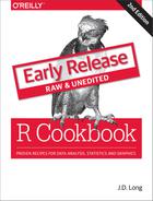
writeData(wb=wb,sheet='input_data',x=paste('example_table data refreshed on:',Sys.time()),startCol=2,startRow=5)## then save the workbooksaveWorkbook(wb=wb,file="data/excel_table_data.xlsx",overwrite=T)
The resulting Excel sheet looks is shown in Figure 4-1.
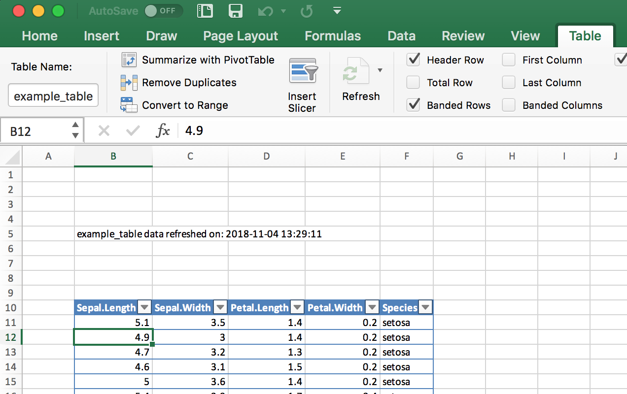
Figure 4-1. Excel Table and Caption
See Also
Vingette for openxlsx by installing openxlsx and running:
vignette(Introduction, package=openxlsx)
The readxl package is party of the Tidyverse and provides fast, simple
reading of Excel files: https://readxl.tidyverse.org/
The writexl package is a fast and lightweight (no dependencies)
package for writing Excel files:
https://cran.r-project.org/web/packages/writexl/index.html
Reading Data from a SAS file
Problem
You want to read a SAS data set into an R data frame.
Solution
The sas7bdat package supports reading SAS sas7bdat files into R.
library(haven)sas_movie_data<-read_sas("data/movies.sas7bdat")
Discussion
SAS V7 and beyond all support the sas7bdat file format. The read_sas
function in haven supports reading the sas7bdat file format including
variable labels. If your SAS file has variable labels, when they are
inported into R they will be stored in the label attributes of the
data frame. These labels will not be printed by default. You can see the
labels by opening the data frame in R Studio, or by calling the
attributes Base R function on each column:
sapply(sas_movie_data,attributes)#> $Movie#> $Movie$label#> [1] "Movie"#>#>#> $Type#> $Type$label#> [1] "Type"#>#>#> $Rating#> $Rating$label#> [1] "Rating"#>#>#> $Year#> $Year$label#> [1] "Year"#>#>#> $Domestic__#> $Domestic__$label#> [1] "Domestic $"#>#> $Domestic__$format.sas#> [1] "F"#>#>#> $Worldwide__#> $Worldwide__$label#> [1] "Worldwide $"#>#> $Worldwide__$format.sas#> [1] "F"#>#>#> $Director#> $Director$label#> [1] "Director"
See Also
The sas7bdat package is much slower on large files than haven, but
it has more elaborate support for file attributes. If the SAS metadata
is important to you then you should investigate
sas7bdat::read.sas7bdat.
Reading Data from HTML Tables
Problem
You want to read data from an HTML table on the Web.
Solution
Use the read_html and html_table functions in the rvest package.
To read all tables on the page, do the following:
library(rvest)library(magrittr)all_tables<-read_html("https://en.wikipedia.org/wiki/Aviation_accidents_and_incidents")%>%html_table(fill=TRUE,header=TRUE)
read_html puts all tables from the HTML document into the output list.
To pull a single table from that list, you can use the function
extract2 from the magrittr package:
out_table<-read_html("https://en.wikipedia.org/wiki/Aviation_accidents_and_incidents")%>%html_table(fill=TRUE,header=TRUE)%>%extract2(2)head(out_table)#> Year Deaths[52] # of incidents[53]#> 1 2017 399 101 [54]#> 2 2016 629 102#> 3 2015 898 123#> 4 2014 1,328 122#> 5 2013 459 138#> 6 2012 800 156
Note that the rvest and magrittr packages are both installed when
you run install.packages('tidyverse') They are not core tidyverse
packages, however, so you must explicitly load them, as shown here.
Discussion
Web pages can contain several HTML tables. Calling read_html(url) then
piping that to html_table() reads all tables on the page and returns
them in a list. This can be useful for exploring a page, but it’s
annoying if you want just one specific table. In that case, use
extract2(n) to select the the _n_th table.
Two common parameters for the html_table function are fill=TRUE
which fills in missing values with NA, and header=TRUE which indicates
that the first row contains the header names.
The following example, loads all tables from the Wikipedia page entitled “World population”:
url<-'http://en.wikipedia.org/wiki/World_population'tbls<-read_html(url)%>%html_table(fill=TRUE,header=TRUE)
As it turns out, that page contains 24 tables (or things that
html_table thinks might be tables):
length(tbls)#> [1] 23
In this example we care only about the sixth table (which lists the
largest populations by country), so we can either access that element
using brackets: tbls[[6]] or we can pipe it into the extract2
function from the magrittr package:
library(magrittr)url<-'http://en.wikipedia.org/wiki/World_population'tbl<-read_html(url)%>%html_table(fill=TRUE,header=TRUE)%>%extract2(2)head(tbl,2)#> World population (millions, UN estimates)[10]#> 1 ##> 2 1#> World population (millions, UN estimates)[10]#> 1 Top ten most populous countries#> 2 China*#> World population (millions, UN estimates)[10]#> 1 2000#> 2 1,270#> World population (millions, UN estimates)[10]#> 1 2015#> 2 1,376#> World population (millions, UN estimates)[10]#> 1 2030*#> 2 1,416
In that table, columns 2 and 3 contain the country name and population, respectively:
tbl[,c(2,3)]#> World population (millions, UN estimates)[10]#> 1 Top ten most populous countries#> 2 China*#> 3 India#> 4 United States#> 5 Indonesia#> 6 Pakistan#> 7 Brazil#> 8 Nigeria#> 9 Bangladesh#> 10 Russia#> 11 Mexico#> 12 World total#> 13 Notes:\nChina = excludes Hong Kong and Macau\n2030 = Medium variant#> World population (millions, UN estimates)[10].1#> 1 2000#> 2 1,270#> 3 1,053#> 4 283#> 5 212#> 6 136#> 7 176#> 8 123#> 9 131#> 10 146#> 11 103#> 12 6,127#> 13 Notes:\nChina = excludes Hong Kong and Macau\n2030 = Medium variant
Right away, we can see problems with the data: the second row of the data has info that really belongs with the header. And China has * appended to its name. On the Wikipedia website, that was a footnote reference, but now it’s just a bit of unwanted text. Adding insult to injury, the population numbers have embedded commas, so you cannot easily convert them to raw numbers. All these problems can be solved by some string processing, but each problem adds at least one more step to the process.
This illustrates the main obstacle to reading HTML tables. HTML was designed for presenting information to people, not to computers. When you “scrape” information off an HTML page, you get stuff that’s useful to people but annoying to computers. If you ever have a choice, choose instead a computer-oriented data representation such as XML, JSON, or CSV.
The read_html(url) and html_table() functions are part of the
rvest package, which (by necessity) is large and complex. Any time you
pull data from a site designed for human readers, not machines, expect
that you will have to do post processing to clean up the bits and pieces
left messy by the machine.
See Also
See “Installing Packages from CRAN” for downloading and installing packages such as the rvest
package.
Reading Files with a Complex Structure
Problem
You are reading data from a file that has a complex or irregular structure.
Solution
-
Use the
readLinesfunction to read individual lines; then process them as strings to extract data items. -
Alternatively, use the
scanfunction to read individual tokens and use the argumentwhatto describe the stream of tokens in your file. The function can convert tokens into data and then assemble the data into records.
Discussion
Life would be simple and beautiful if all our data files were organized
into neat tables with cleanly delimited data. We could read those files
using one of the functions in the readr package and get on with
living.
Unfortunatly we don’t live in a land of rainbows and unicorn kisses.
You will eventually encounter a funky file format, and your job (suck it up, buttercup) is to read the file contents into R.
The read.table and read.csv functions are line-oriented and probably
won’t help. However, the readLines and scan functions are useful
here because they let you process the individual lines and even tokens
of the file.
The readLines function is pretty simple. It reads lines from a file
and returns them as a list of character strings:
lines<-readLines("input.txt")
You can limit the number of lines by using the n parameter, which
gives the number of maximum number of lines to be read:
lines<-readLines("input.txt",n=10)# Read 10 lines and stop
The scan function is much richer. It reads one token at a time and
handles it according to your instructions. The first argument is either
a filename or a connection (more on connections later). The second
argument is called what, and it describes the tokens that scan
should expect in the input file. The description is cryptic but quite
clever:
what=numeric(0)-
Interpret the next token as a number.
what=integer(0)-
Interpret the next token as an integer.
what=complex(0)-
Interpret the next token as complex number.
what=character(0)-
Interpret the next token as a character string.
what=logical(0)-
Interpret the next token as a logical value.
The scan function will apply the given pattern repeatedly until all
data is read.
Suppose your file is simply a sequence of numbers, like this:
2355.09 2246.73 1738.74 1841.01 2027.85
Use what=numeric(0) to say, “My file is a sequence of tokens, each of
which is a number”:
singles<-scan("./data/singles.txt",what=numeric(0))singles#> [1] 2355.09 2246.73 1738.74 1841.01 2027.85
A key feature of scan is that the what can be a list containing
several token types. The scan function will assume your file is a
repeating sequence of those types. Suppose your file contains triplets
of data, like this:
15-Oct-87 2439.78 2345.63 16-Oct-87 2396.21 2207.73
19-Oct-87 2164.16 1677.55 20-Oct-87 2067.47 1616.21
21-Oct-87 2081.07 1951.76
Use a list to tell scan that it should expect a repeating, three-token
sequence:
triples<-scan("./data/triples.txt",what=list(character(0),numeric(0),numeric(0)))triples#> [[1]]#> [1] "15-Oct-87" "16-Oct-87" "19-Oct-87" "20-Oct-87" "21-Oct-87"#>#> [[2]]#> [1] 2439.78 2396.21 2164.16 2067.47 2081.07#>#> [[3]]#> [1] 2345.63 2207.73 1677.55 1616.21 1951.76
Give names to the list elements, and scan will assign those names to
the data:
triples<-scan("./data/triples.txt",what=list(date=character(0),high=numeric(0),low=numeric(0)))triples#> $date#> [1] "15-Oct-87" "16-Oct-87" "19-Oct-87" "20-Oct-87" "21-Oct-87"#>#> $high#> [1] 2439.78 2396.21 2164.16 2067.47 2081.07#>#> $low#> [1] 2345.63 2207.73 1677.55 1616.21 1951.76
This can easily be turned into a data frame with the data.frame
command:
df_triples<-data.frame(triples)df_triples#> date high low#> 1 15-Oct-87 2439.78 2345.63#> 2 16-Oct-87 2396.21 2207.73#> 3 19-Oct-87 2164.16 1677.55#> 4 20-Oct-87 2067.47 1616.21#> 5 21-Oct-87 2081.07 1951.76
The scan function has many bells and whistles, but the following are
especially useful:
n=number-
Stop after reading this many tokens. (Default: stop at end of file.)
nlines=number-
Stop after reading this many input lines. (Default: stop at end of file.)
skip=number-
Number of input lines to skip before reading data.
na.strings=list-
A list of strings to be interpreted as NA.
An Example
Let’s use this recipe to read a dataset from StatLib, the repository of
statistical data and software maintained by Carnegie Mellon University.
Jeff Witmer contributed a dataset called wseries that shows the
pattern of wins and losses for every World Series since 1903. The
dataset is stored in an ASCII file with 35 lines of comments followed by
23 lines of data. The data itself looks like this:
1903  LWLlwwwW    1927  wwWW      1950  wwWW      1973  WLwllWW
1905  wLwWW       1928  WWww      1951  LWlwwW    1974  wlWWW
1906  wLwLwW      1929  wwLWW     1952  lwLWLww   1975  lwWLWlw
1907  WWww        1930  WWllwW    1953  WWllwW    1976  WWww
1908  wWLww       1931  LWwlwLW   1954  WWww      1977  WLwwlW

.
. (etc.)
.
The data is encoded as follows: L = loss at home, l = loss on the road, W = win at home, w = win on the road. The data appears in column order, not row order, which complicates our lives a bit.
Here is the R code for reading the raw data:
# Read the wseries dataset:# - Skip the first 35 lines# - Then read 23 lines of data# - The data occurs in pairs: a year and a pattern (char string)#world.series<-scan("http://lib.stat.cmu.edu/datasets/wseries",skip=35,nlines=23,what=list(year=integer(0),pattern=character(0)),)
The scan function returns a list, so we get a list with two elements:
year and pattern. The function reads from left to right, but the
dataset is organized by columns and so the years appear in a strange
order:
world.series$year#> [1] 1903 1927 1950 1973 1905 1928 1951 1974 1906 1929 1952 1975 1907 1930#> [15] 1953 1976 1908 1931 1954 1977 1909 1932 1955 1978 1910 1933 1956 1979#> [29] 1911 1934 1957 1980 1912 1935 1958 1981 1913 1936 1959 1982 1914 1937#> [43] 1960 1983 1915 1938 1961 1984 1916 1939 1962 1985 1917 1940 1963 1986#> [57] 1918 1941 1964 1987 1919 1942 1965 1988 1920 1943 1966 1989 1921 1944#> [71] 1967 1990 1922 1945 1968 1991 1923 1946 1969 1992 1924 1947 1970 1993#> [85] 1925 1948 1971 1926 1949 1972
We can fix that by sorting the list elements according to year:
perm<-order(world.series$year)world.series<-list(year=world.series$year[perm],pattern=world.series$pattern[perm])
Now the data appears in chronological order:
world.series$year#> [1] 1903 1905 1906 1907 1908 1909 1910 1911 1912 1913 1914 1915 1916 1917#> [15] 1918 1919 1920 1921 1922 1923 1924 1925 1926 1927 1928 1929 1930 1931#> [29] 1932 1933 1934 1935 1936 1937 1938 1939 1940 1941 1942 1943 1944 1945#> [43] 1946 1947 1948 1949 1950 1951 1952 1953 1954 1955 1956 1957 1958 1959#> [57] 1960 1961 1962 1963 1964 1965 1966 1967 1968 1969 1970 1971 1972 1973#> [71] 1974 1975 1976 1977 1978 1979 1980 1981 1982 1983 1984 1985 1986 1987#> [85] 1988 1989 1990 1991 1992 1993world.series$pattern#> [1] "LWLlwwwW" "wLwWW" "wLwLwW" "WWww" "wWLww" "WLwlWlw"#> [7] "WWwlw" "lWwWlW" "wLwWlLW" "wLwWw" "wwWW" "lwWWw"#> [13] "WWlwW" "WWllWw" "wlwWLW" "WWlwwLLw" "wllWWWW" "LlWwLwWw"#> [19] "WWwW" "LwLwWw" "LWlwlWW" "LWllwWW" "lwWLLww" "wwWW"#> [25] "WWww" "wwLWW" "WWllwW" "LWwlwLW" "WWww" "WWlww"#> [31] "wlWLLww" "LWwwlW" "lwWWLw" "WWwlw" "wwWW" "WWww"#> [37] "LWlwlWW" "WLwww" "LWwww" "WLWww" "LWlwwW" "LWLwwlw"#> [43] "LWlwlww" "WWllwLW" "lwWWLw" "WLwww" "wwWW" "LWlwwW"#> [49] "lwLWLww" "WWllwW" "WWww" "llWWWlw" "llWWWlw" "lwLWWlw"#> [55] "llWLWww" "lwWWLw" "WLlwwLW" "WLwww" "wlWLWlw" "wwWW"#> [61] "WLlwwLW" "llWWWlw" "wwWW" "wlWWLlw" "lwLLWww" "lwWWW"#> [67] "wwWLW" "llWWWlw" "wwLWLlw" "WLwllWW" "wlWWW" "lwWLWlw"#> [73] "WWww" "WLwwlW" "llWWWw" "lwLLWww" "WWllwW" "llWWWw"#> [79] "LWwllWW" "LWwww" "wlWWW" "LLwlwWW" "LLwwlWW" "WWlllWW"#> [85] "WWlww" "WWww" "WWww" "WWlllWW" "lwWWLw" "WLwwlW"
Reading from MySQL Databases
Problem
You want access to data stored in a MySQL database.
Solution
-
Install the
RMySQLpackage on your computer. -
Open a database connection using the
DBI::dbConnectfunction. -
Use
dbGetQueryto initiate aSELECTand return the result sets. -
Use
dbDisconnectto terminate the database connection when you are done.
Discussion
This recipe requires that the RMySQL package be installed on your
computer. That package requires, in turn, the MySQL client software. If
the MySQL client software is not already installed and configured,
consult the MySQL documentation or your system administrator.
Use the dbConnect function to establish a connection to the MySQL
database. It returns a connection object which is used in subsequent
calls to RMySQL functions:
library(RMySQL)con<-dbConnect(drv=RMySQL::MySQL(),dbname="your_db_name",host="your.host.com",username="userid",password="pwd")
The username, password, and host parameters are the same parameters used
for accessing MySQL through the mysql client program. The example
given here shows them hard-coded into the dbConnect call. Actually,
that is an ill-advised practice. It puts your password in a plain text
document, creating a security problem. It also creates a major headache
whenever your password or host change, requiring you to hunt down the
hard-coded values. I strongly recommend using the security mechanism of
MySQL instead. Put those three parameters into your MySQL configuration
file, which is $HOME/.my.cnf on Unix and C:\my.cnf on Windows. Make
sure the file is unreadable by anyone except you. The file is delimited
into sections with markers such as [client]. Put the parameters into
the [client] section, so that your config file will contain something
like this:
[client]
user = userid
password = password
host = hostname
Once the parameters are defined in the config file, you no longer need
to supply them in the dbConnect call, which then becomes much simpler:
-
jal TODO - test this in anger
con<-dbConnect(dbConnect(drv=RMySQL::MySQL(),dbname="your_db_name",host="your.host.com")
Use the dbGetQuery function to submit your SQL to the database and
read the result sets. Doing so requires an open database connection:
sql<-"SELECT * from SurveyResults WHERE City = 'Chicago'"rows<-dbGetQuery(con,sql)
You are not restricted to SELECT statements. Any SQL that generates a
result set is OK. It is common to use CALL statements, for example, if
your SQL is encapsulated in stored procedures and those stored
procedures contain embedded SELECT statements.
Using dbGetQuery is convenient because it packages the result set into
a data frame and returns the data frame. This is the perfect
representation of an SQL result set. The result set is a tabular data
structure of rows and columns, and so is a data frame. The result set’s
columns have names given by the SQL SELECT statement, and R uses them
for naming the columns of the data frame.
After the first result set of data, MySQL can return a second result set
containing status information. You can choose to inspect the status or
ignore it, but you must read it. Otherwise, MySQL will complain that
there are unprocessed result sets and then halt. So call dbNextResult
if necessary:
if(dbMoreResults(con))dbNextResult(con)
Call dbGetQuery repeatedly to perform multiple queries, checking for
the result status after each call (and reading it, if necessary). When
you are done, close the database connection using dbDisconnect:
dbDisconnect(con)
Here is a complete session that reads and prints three rows from a
database of stock prices. The query selects the price of IBM stock for
the last three days of 2008. It assumes that the username, password, and
host are defined in the my.cnf file:
con<-dbConnect(MySQL(),client.flag=CLIENT_MULTI_RESULTS)sql<-paste("select * from DailyBar where Symbol = 'IBM'","and Day between '2008-12-29' and '2008-12-31'")rows<-dbGetQuery(con,sql)if(dbMoreResults(con)){dbNextResults(con)}dbDisconnect(con)(rows)
*TODO - format this so it looks like output, maybe? * TODO - do we need the dbMoreResults still? Symbol Day Next OpenPx HighPx LowPx ClosePx AdjClosePx 1 IBM 2008-12-29 2008-12-30 81.72 81.72 79.68 81.25 81.25 2 IBM 2008-12-30 2008-12-31 81.83 83.64 81.52 83.55 83.55 3 IBM 2008-12-31 2009-01-02 83.50 85.00 83.50 84.16 84.16 HistClosePx Volume OpenInt 1 81.25 6062600 NA 2 83.55 5774400 NA 3 84.16 6667700 NA
See Also
See “Installing Packages from CRAN” and the documentation for RMySQL, which contains more
details about configuring and using the package.
See “Accessing a Database with dbplyr” for information about how to get data from an SQL without actually writing SQL yourself.
R can read from several other RDBMS systems, including Oracle, Sybase, PostgreSQL, and SQLite. For more information, see the R Data Import/Export guide, which is supplied with the base distribution (“Viewing the Supplied Documentation”) and is also available on CRAN at http://cran.r-project.org/doc/manuals/R-data.pdf.
Accessing a Database with dbplyr
Problem
You want to access a database, but you’d rather not write SQL code in order to manipulate data and return results to R.
Solution
In addition to being a grammar of data manipulation, the tidyverse
package dplyr can, in in connection with the dbplyr package, turn
dplyr commands into SQL for you.
Let’s set up an example database using RSQLite and then we’ll connect
to it and use dplyr and the dbplyr backend to extract data.
Set up the example table by loading the msleep example data into an
in-memory SQLite database:
con<-DBI::dbConnect(RSQLite::SQLite(),":memory:")sleep_db<-copy_to(con,msleep,"sleep")
Now that we have a table in our database, we can create a reference to
it from R
sleep_table<-tbl(con,"sleep")
The sleep_table object is a type of pointer or alias to the table on
the database. However, dplyr will treat it like a regular tidyverse
tibble or data frame. So you can operate on it using dplyr and other R
commands. Let’s select all anaimals from the data who sleep less than 3
hours.
little_sleep<-sleep_table%>%select(name,genus,order,sleep_total)%>%filter(sleep_total<3)
The dbplyr backend does not go fetch the data when we do the above
commands. But it does build the query and get ready. To see the query
built by dplyr you can use show_query:
show_query(little_sleep)#> <SQL>#> SELECT *#> FROM (SELECT `name`, `genus`, `order`, `sleep_total`#> FROM `sleep`)#> WHERE (`sleep_total` < 3.0)
Then to bring the data back to your local machine use collect:
local_little_sleep<-collect(little_sleep)local_little_sleep#> # A tibble: 3 x 4#> name genus order sleep_total#> <chr> <chr> <chr> <dbl>#> 1 Horse Equus Perissodactyla 2.9#> 2 Giraffe Giraffa Artiodactyla 1.9#> 3 Pilot whale Globicephalus Cetacea 2.7
Discussion
By using dplyr to access SQL databases by only writing dplyr commands, you can be more productive by not having to switch from one language to another and back. The alternative is to have large chunks of SQL code stored as text strings in the middle of an R script, or have the SQL in seperate files which are read in by R.
By allowing dplyr to transparently create the SQL in the background, the user is freed from having to maintain seperate SQL code to extract data.
The dbplyr package uses DBI to connect to your database, so you’ll need a DBI backend package for whichever database you want to access.
Some commonly used backend DBI packages are:
- odbc
-
Uses the open database connectivity protocol to connect to many different databases. This is typically the best choice when connecting to Microsoft SQL Server. ODBC is typically straight forward on Windows machines but may require some considerable effort to get working in Linux or Mac.
- RPostgreSQL
-
For connecting to Postgres and Redshift.
- RMySQL
-
For MySQL and MariaDB
- RSQLite
-
Connecting to SQLite databases on disk or in memory.
- bigrquery
-
For connections to Google’s BigQuery.
Each DBI backend package listed above is listed on CRAN and can be
installed with the typical install.packages('packagename') command.
See Also
For more information about connecting the databases with R & RStudio: https://db.rstudio.com/
For more detail on SQL translation in dbplyr, see the sql-translation
vignette at vignette("sql-translation") or
http://dbplyr.tidyverse.org/articles/sql-translation.html
Saving and Transporting Objects
Problem
You want to store one or more R objects in a file for later use, or you want to copy an R object from one machine to another.
Solution
Write the objects to a file using the save function:
save(tbl,t,file="myData.RData")
Read them back using the load function, either on your computer or on
any platform that supports R:
load("myData.RData")
The save function writes binary data. To save in an ASCII format, use
dput or dump instead:
dput(tbl,file="myData.txt")dump("tbl",file="myData.txt")# Note quotes around variable name
Discussion
We’ve found ourselves with a large, complicated data object that we want
to load into other workspaces, or we may want to move R objects between
a Linux box and a Windows box. The load and save functions let us do
all this: save will store the object in a file that is portable across
machines, and load can read those files.
When you run load, it does not return your data per se; rather, it
creates variables in your workspace, loads your data into those
variables, and then returns the names of the variables (in a vector).
The first time you run load, you might be tempted to do this:
myData<-load("myData.RData")# Achtung! Might not do what you think
Let’s look at what myData is above:
myData#> [1] "tbl" "t"str(myData)#> chr [1:2] "tbl" "t"
This might be puzzling, because myData will not contain your data at
all. This can be perplexing and frustrating the first time.
The save function writes in a binary format to keep the file small.
Sometimes you want an ASCII format instead. When you submit a question
to a mailing list or to Stack Overflow, for example, including an ASCII
dump of the data lets others re-create your problem. In such cases use
dput or dump, which write an ASCII representation.
Be careful when you save and load objects created by a particular R
package. When you load the objects, R does not automatically load the
required packages, too, so it will not “understand” the object unless
you previously loaded the package yourself. For instance, suppose you
have an object called z created by the zoo package, and suppose we
save the object in a file called z.RData. The following sequence of
functions will create some confusion:
load("./data/z.RData")# Create and populate the z variableplot(z)# Does not plot as expected: zoo pkg not loaded
We should have loaded the zoo package before printing or plotting
any zoo objects, like this:
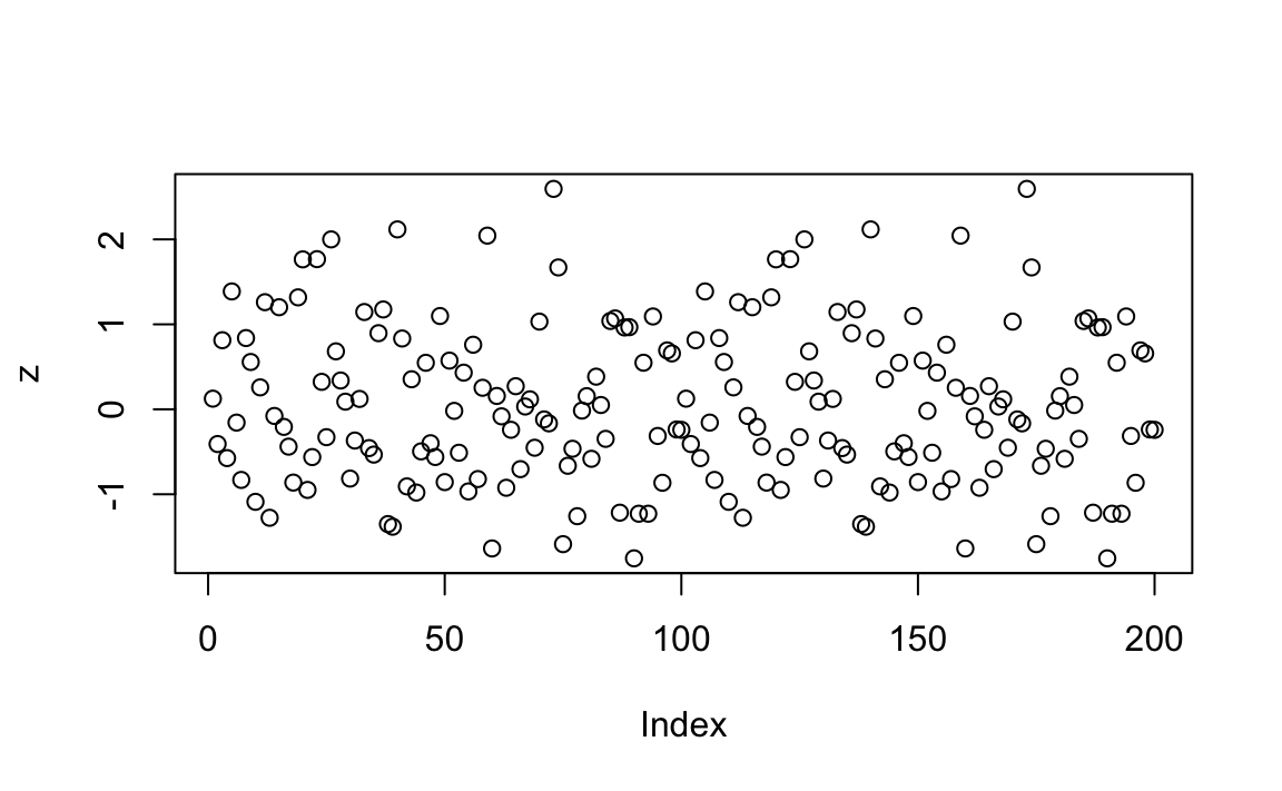
library(zoo)# Load the zoo package into memoryload("./data/z.RData")# Create and populate the z variableplot(z)# Ahhh. Now plotting works correctly
Figure 4-2. Plotting with zoo
And you can see the resulting plot in Figure 4-2.