Second Edition
Proven Recipes for Data Analysis, Statistics, and Graphics
Copyright © 2019 J.D. Long and Paul Teetor. All rights reserved.
Printed in the United States of America.
Published by O’Reilly Media, Inc., 1005 Gravenstein Highway North, Sebastopol, CA 95472.
O’Reilly books may be purchased for educational, business, or sales promotional use. Online editions are also available for most titles (http://oreilly.com/safari). For more information, contact our corporate/institutional sales department: 800-998-9938 or corporate@oreilly.com.
See http://oreilly.com/catalog/errata.csp?isbn=9781492040682 for release details.
The O’Reilly logo is a registered trademark of O’Reilly Media, Inc. R Cookbook, the cover image, and related trade dress are trademarks of O’Reilly Media, Inc.
While the publisher and the author have used good faith efforts to ensure that the information and instructions contained in this work are accurate, the publisher and the author disclaim all responsibility for errors or omissions, including without limitation responsibility for damages resulting from the use of or reliance on this work. Use of the information and instructions contained in this work is at your own risk. If any code samples or other technology this work contains or describes is subject to open source licenses or the intellectual property rights of others, it is your responsibility to ensure that your use thereof complies with such licenses and/or rights.
978-1-492-04068-2
This chapter sets the groundwork for the other chapters. It explains how to download, install, and run R.
More importantly, it also explains how to get answers to your questions. The R community provides a wealth of documentation and help. You are not alone. Here are some common sources of help:
When you install R on your computer, a mass of documentation is also installed. You can browse the local documentation (“Viewing the Supplied Documentation”) and search it (“Searching the Supplied Documentation”). We are amazed how often we search the Web for an answer only to discover it was already available in the installed documentation.
A task view describes packages that are specific to one area of statistical work, such as econometrics, medical imaging, psychometrics, or spatial statistics. Each task view is written and maintained by an expert in the field. There are more than 35 such task views, so there is likely to be one or more for your areas of interest. We recommend that every beginner find and read at least one task view in order to gain a sense of R’s possibilities (“Finding Relevant Functions and Packages”).
Most packages include useful documentation. Many also include overviews and tutorials, called “vignettes” in the R community. The documentation is kept with the packages in package repositories, such as CRAN (http://cran.r-project.org/), and it is automatically installed on your machine when you install a package.
On a Q&A site, anyone can post a question, and knowledgeable people can respond. Readers vote on the answers, so the best answers tend to emerge over time. All this information is tagged and archived for searching. These sites are a cross between a mailing list and a social network; “Stack Overflow” (http://stackoverflow.com/) is the canonical example.
The Web is loaded with information about R, and there are R-specific tools for searching it (“Searching the Web for Help”). The Web is a moving target, so be on the lookout for new, improved ways to organize and search information regarding R.
Volunteers have generously donated many hours of time to answer beginners’ questions that are posted to the R mailing lists. The lists are archived, so you can search the archives for answers to your questions (“Searching the Mailing Lists”).
You want to install R on your computer.
Windows and OS X users can download R from CRAN, the Comprehensive R Archive Network. Linux and Unix users can install R packages using their package management tool:
Windows
Open http://www.r-project.org/ in your browser.
Click on “CRAN”. You’ll see a list of mirror sites, organized by country.
Select a site near you or the top one listed as “0-Cloud” which tends to work well for most locations (https://cloud.r-project.org/)
Click on “Download R for Windows” under “Download and Install R”.
Click on “base”.
Click on the link for downloading the latest version of R (an .exe
file).
When the download completes, double-click on the .exe file and
answer the usual questions.
OS X
Open http://www.r-project.org/ in your browser.
Click on “CRAN”. You’ll see a list of mirror sites, organized by country.
Select a site near you or the top one listed as “0-Cloud” which tends to work well for most locations.
Click on “Download R for (Mac) OS X”.
Click on the .pkg file for the latest version of R, under “Latest
release:”, to download it.
When the download completes, double-click on the .pkg file and
answer the usual questions.
Linux or Unix
The major Linux distributions have packages for installing R. Here are some examples:
| Distribution | Package name |
|---|---|
Ubuntu or Debian |
r-base |
Red Hat or Fedora |
R.i386 |
Suse |
R-base |
Use the system’s package manager to download and install the package.
Normally, you will need the root password or sudo privileges;
otherwise, ask a system administrator to perform the installation.
Installing R on Windows or OS X is straightforward because there are prebuilt binaries (compiled programs) for those platforms. You need only follow the preceding instructions. The CRAN Web pages also contain links to installation-related resources, such as frequently asked questions (FAQs) and tips for special situations (“Does R run under Windows Vista/7/8/Server 2008?”) that you may find useful.
The best way to install R on Linux or Unix is by using your Linux distribution package manager to install R as a package. The distribution packages greatly streamline both the initial installation and subsequent updates.
On Ubuntu or Debian, use apt-get to download and install R. Run under
sudo to have the necessary privileges:
$sudoapt-getinstallr-base
On Red Hat or Fedora, use yum:
$sudoyuminstallR.i386
Most Linux platforms also have graphical package managers, which you might find more convenient.
Beyond the base packages, we recommend installing the documentation
packages, too. We like to install r-base-html (because we like
browsing the hyperlinked documentation) as well as r-doc-html, which
installs the important R manuals locally:
$sudoapt-getinstallr-base-htmlr-doc-html
Some Linux repositories also include prebuilt copies of R packages available on CRAN. We don’t use them because we’d rather get software directly from CRAN itself, which usually has the freshest versions.
In rare cases, you may need to build R from scratch. You might have an
obscure, unsupported version of Unix; or you might have special
considerations regarding performance or configuration. The build
procedure on Linux or Unix is quite standard. Download the tarball from
the home page of your CRAN mirror; it’s called something like
R-3.5.1.tar.gz, except the “3.5.1” will be replaced by the latest
version. Unpack the tarball, look for a file called INSTALL, and
follow the directions.
R in a Nutshell (http://oreilly.com/catalog/9780596801717) (O’Reilly) contains more details of downloading and installing R, including instructions for building the Windows and OS X versions. Perhaps the ultimate guide is the one entitled “R Installation and Administration” (http://cran.r-project.org/doc/manuals/R-admin.html), available on CRAN, which describes building and installing R on a variety of platforms.
This recipe is about installing the base package. See “Installing Packages from CRAN” for installing add-on packages from CRAN.
You want a more comprehensive Integrated Development Environment (IDE) than the R default. In other words, you want to install R Studio Desktop.
Over the past few years R Studio has become the most widly used IDE for
R. We are of the opinion that most all R work should be done in the R
Studio Desktop IDE unless there is a compelling reason to do otherwise.
R Studio makes multiple products including R Studio Desktop, R Studio
Server, R Studio Shiny Server, just to name a few. For this book we will
use the term R Studio to mean R Studio Desktop though most concepts
apply to R Studio Server as well.
To install R Studio, download the latest installer for your platform from the R Studio website: https://www.rstudio.com/products/rstudio/download/
The R Studio Desktop Open Source License version is free to download and use.
This book was written and built using R Studio version 1.2.x and R versions 3.5.x. New versions of R Studio are released every few months, so be sure and update regularly. Note that R Studio works with whichever version of R you have installed. So updating to the latest version of R Studio does not upgrade your version of R. R must be upgraded seperatly.
Interacting with R is slightly different in R Studio than in the built in R user interface. For this book, we’ve elected to use R Studio for all examples.
You want to run R Studio on your computer.
A common point of confusion for new users of R and R Studio is to
accidentally start R when they intended to start R Studio. The easiest
way to ensure you’re actually starting R Studio is to search for
RStudio on your desktop OS. Then use whatever method your OS provides
for pinning the icon somewhere easy to find later.
Click on the Start Screen menue in the lower left corner of the
screen. In the search box, type RStudio.
Look in your launchpad for the R Studio app or press command
space and type Rstudio to search using Spotlight Search.
Press Alt + F1 and type RStudio to search for R Studio.
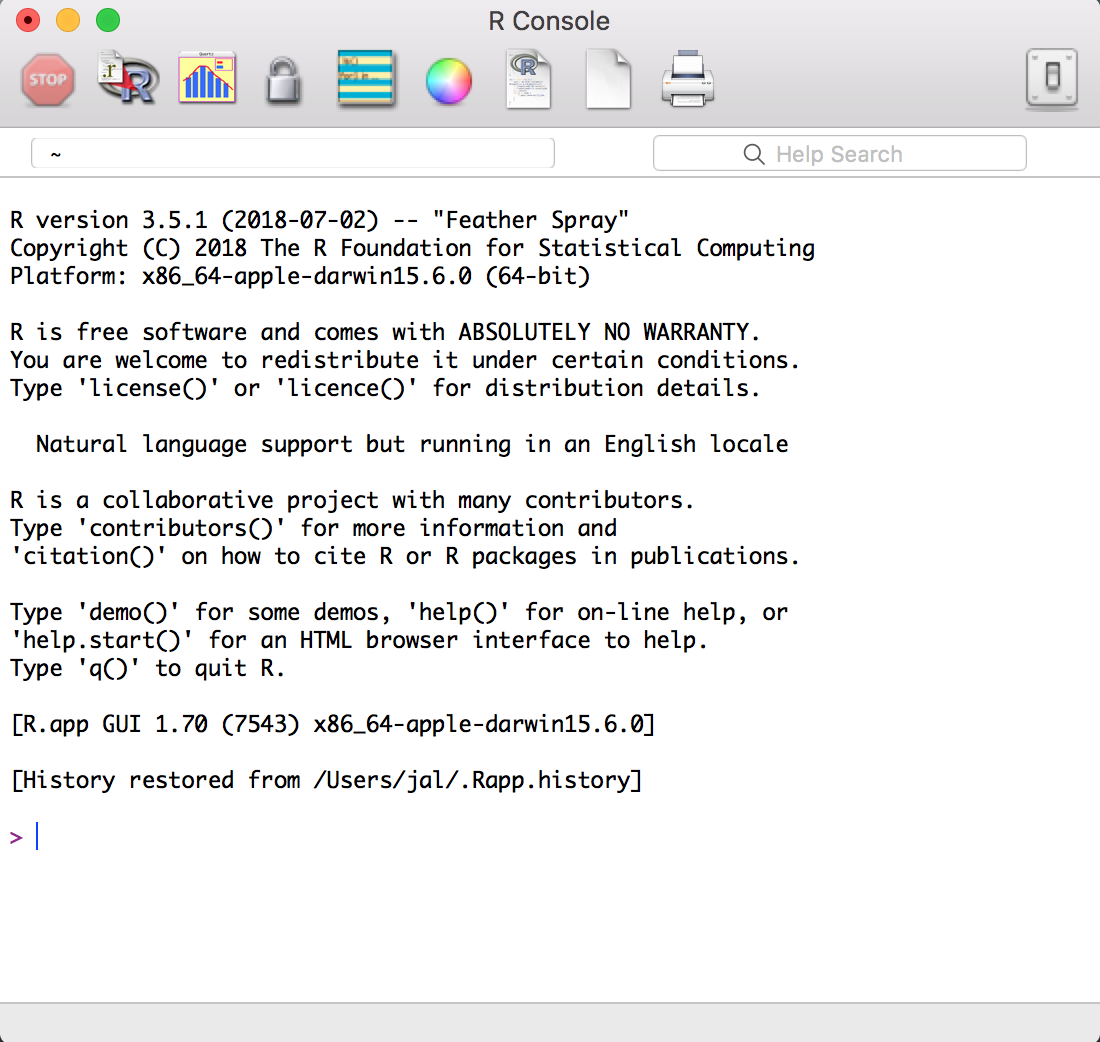
Confusion between R and R Studio can easily happen becuase as you can see in Figure 1-1, the icons look similiar.

If you click on the R icon you’ll be greeted by something like Figure
Figure 1-2 which is the Base R interface on a Mac, but certainly
not R Studio.
When you start R Studio, the default behavior is that R Studio will reopen the last project you were working on in R Studio.
You’ve started R Studio. Now what?
When you start R Studio, the main window on the left is an R session. From there you can enter commands interactivly directly to R.
R prompts you with “>”. To get started, just treat R like a big
calculator: enter an expression, and R will evaluate the expression and
print the result:
1+1#> [1] 2
The computer adds one and one, giving two, and displays the result.
The [1] before the 2 might be confusing. To R, the result is a
vector, even though it has only one element. R labels the value with
[1] to signify that this is the first element of the vector… which
is not surprising, since it’s the only element of the vector.
R will prompt you for input until you type a complete expression. The
expression max(1,3,5) is a complete expression, so R stops reading
input and evaluates what it’s got:
max(1,3,5)#> [1] 5
In contrast, “max(1,3,” is an incomplete expression, so R prompts you
for more input. The prompt changes from greater-than (>) to plus
(+), letting you know that R expects more:
max(1,3,+5)#> [1] 5
It’s easy to mistype commands, and retyping them is tedious and frustrating. So R includes command-line editing to make life easier. It defines single keystrokes that let you easily recall, correct, and reexecute your commands. My own typical command-line interaction goes like this:
I enter an R expression with a typo.
R complains about my mistake.
I press the up-arrow key to recall my mistaken line.
I use the left and right arrow keys to move the cursor back to the error.
I use the Delete key to delete the offending characters.
I type the corrected characters, which inserts them into the command line.
I press Enter to reexecute the corrected command.
That’s just the basics. R supports the usual keystrokes for recalling and editing command lines, as listed in table @ref(tab:keystrokes).
| Labeled key | Ctrl-key combination | Effect |
|---|---|---|
Up arrow |
Ctrl-P |
Recall previous command by moving backward through the history of commands. |
Down arrow |
Ctrl-N |
Move forward through the history of commands. |
Backspace |
Ctrl-H |
Delete the character to the left of cursor. |
Delete (Del) |
Ctrl-D |
Delete the character to the right of cursor. |
Home |
Ctrl-A |
Move cursor to the start of the line. |
End |
Ctrl-E |
Move cursor to the end of the line. |
Right arrow |
Ctrl-F |
Move cursor right (forward) one character. |
Left arrow |
Ctrl-B |
Move cursor left (back) one character. |
Ctrl-K |
Delete everything from the cursor position to the end of the line. |
|
Ctrl-U |
Clear the whole darn line and start over. |
|
Tab |
Name completion (on some platforms). |
: Keystrokes for command-line editing
On Windows and OS X, you can also use the mouse to highlight commands and then use the usual copy and paste commands to paste text into a new command line.
See “Typing Less and Accomplishing More”. From the Windows main menu, follow Help →
Console for a complete list of keystrokes useful for command-line
editing.
You want to exit from R Studio.
Select File → Quit Session from the main menu; or click on the X
in the upper-right corner of the window frame.
Press CMD-q (apple-q); or click on the red X in the upper-left corner of the window frame.
At the command prompt, press Ctrl-D.
On all platforms, you can also use the q function (as in _q_uit) to
terminate the program.
q()
Note the empty parentheses, which are necessary to call the function.
Whenever you exit, R typically asks if you want to save your workspace. You have three choices:
Save your workspace and exit.
Don’t save your workspace, but exit anyway.
Cancel, returning to the command prompt rather than exiting.
If you save your workspace, then R writes it to a file called .RData
in the current working directory. Savign the workspace saves any R
objects which you have created. Next time you start R in the same
directory the workspace will automatically load. Saving your workspace
will overwrite the previously saved workspace, if any, so don’t save if
you don’t like the changes to your workspace (e.g., if you have
accidentally erased critical data).
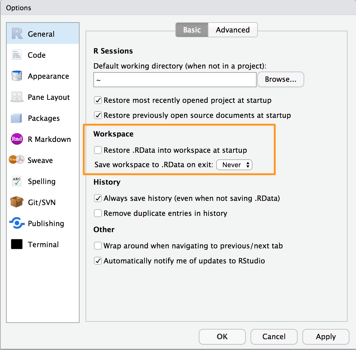
We recommend never saving your workspace when you exit, and instead
always explicitly saving your project, scripts, and data. We also
recommend that you turn off the prompt to save and auto restore of
workspace in R Studio using the Global Options found in the menu Tools
→ Global Options and shown in Figure 1-3. This way
when you exit R and R Studio you will not be prompted to save your
workspace. But keep in mind that any objects created but not saved to
disk will be lost.
See “Getting and Setting the Working Directory” for more about the current working directory and “Saving Your Workspace” for more about saving your workspace. See Chapter 2 of R in a Nutshell (http://oreilly.com/catalog/9780596801717).
You want to interrupt a long-running computation and return to the command prompt without exiting R Studio.
Press the Esc key on your keyboard, or click on the Session Menu in
R Studio and select Interrupt R
Interrupting R means telling R to stop running the current command but without deleting variables from memory or completly closing R Studio. Although, interrupting R can leave your variables in an indeterminate state, depending upon how far the computation had progressed. Check your workspace after interrupting.
You want to read the documentation supplied with R.
Use the help.start function to see the documentation’s table of
contents:
help.start()
From there, links are available to all the installed documentation. In R Studio the help will show up in the help pane which by default is on the right hand side of the screen.
In R Studio you can also click help → R Help to get a listng with
help options for both R and R Studio.
The base distribution of R includes a wealth of documentation—literally thousands of pages. When you install additional packages, those packages contain documentation that is also installed on your machine.
It is easy to browse this documentation via the help.start function,
which opens on the top-level table of contents. Figure
Figure 1-4 shows how help.start() appears inside the help
pane in R Studio.
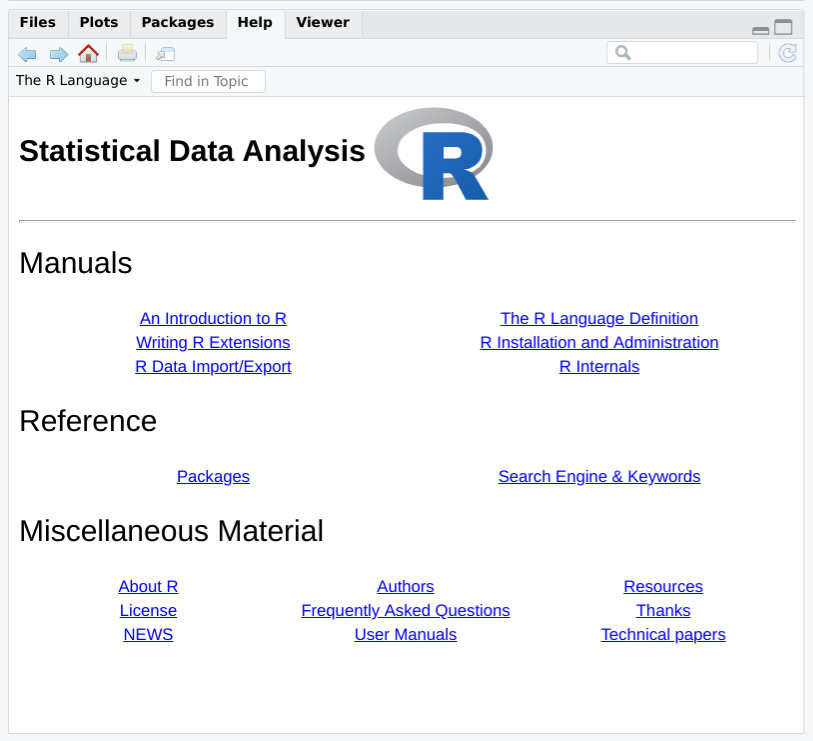
The two links in the Base R Reference section are especially useful:
Click here to see a list of all the installed packages, both in the base packages and the additional, installed packages. Click on a package name to see a list of its functions and datasets.
Click here to access a simple search engine, which allows you to search the documentation by keyword or phrase. There is also a list of common keywords, organized by topic; click one to see the associated pages.
The Base R documentation shown by typing help.start() is loaded on
your computer when you install R. The R Studio help which you get by
using the menu option help → R Help presents a page with links to R
Studio’s web site. So you will need Internet access to access the R
Studio help links.
The local documentation is copied from the R Project website, which may have updated documents.
You want to know more about a function that is installed on your machine.
Use help to display the documentation for the function:
help(functionname)
Use args for a quick reminder of the function arguments:
args(functionname)
Use example to see examples of using the function:
example(functionname)
We present many R functions in this book. Every R function has more bells and whistles than we can possibly describe. If a function catches your interest, we strongly suggest reading the help page for that function. One of its bells or whistles might be very useful to you.
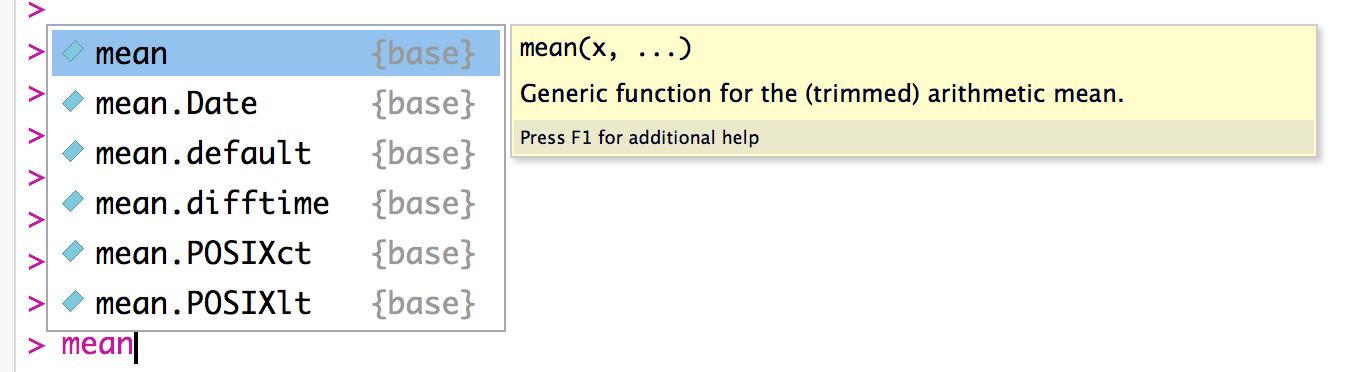
Suppose you want to know more about the mean function. Use the help
function like this:
help(mean)
This will open the help page for the mean function in the help pane in R
Studio. A shortcut for the help command is to simply type ? followed
by the function name:
?mean
Sometimes you just want a quick reminder of the arguments to a function:
What are they, and in what order do they occur? Use the args function:
args(mean)#> function (x, ...)#> NULL
args(sd)#> function (x, na.rm = FALSE)#> NULL
The first line of output from args is a synopsis of the function call.
For mean, the synopsis shows one argument, x, which is a vector of
numbers. For sd, the synopsis shows the same vector, x, and an
optional argument called na.rm. (You can ignore the second line of
output, which is often just NULL.) In R Studio you will see the args
output as a floating tool tip over your cursor when you type a function
name as shown in figure Figure 1-5.
Most documentation for functions includes example code near the end of
the document. A cool feature of R is that you can request that it
execute the examples, giving you a little demonstration of the
function’s capabilities. The documentation for the mean function, for
instance, contains examples, but you don’t need to type them yourself.
Just use the example function to watch them run:
example(mean)#>#> mean> x <- c(0:10, 50)#>#> mean> xm <- mean(x)#>#> mean> c(xm, mean(x, trim = 0.10))#> [1] 8.75 5.50
The user typed example(mean). Everything else was produced by R, which
executed the examples from the help page and displayed the results.
See “Searching the Supplied Documentation” for searching for functions and “Displaying Loaded Packages via the Search Path” for more about the search path.
You want to know more about a function that is installed on your
machine, but the help function reports that it cannot find
documentation for any such function.
Alternatively, you want to search the installed documentation for a keyword.
Use help.search to search the R documentation on your computer:
help.search("pattern")
A typical pattern is a function name or keyword. Notice that it must be enclosed in quotation marks.
For your convenience, you can also invoke a search by using two question marks (in which case the quotes are not required). Note that searching for a function by name uses one question mark while searching for a text pattern uses two:
>??pattern
You may occasionally request help on a function only to be told R knows nothing about it:
help(adf.test)#> No documentation for 'adf.test' in specified packages and libraries:#> you could try '??adf.test'
This can be frustrating if you know the function is installed on your machine. Here the problem is that the function’s package is not currently loaded, and you don’t know which package contains the function. It’s a kind of catch-22 (the error message indicates the package is not currently in your search path, so R cannot find the help file; see “Displaying Loaded Packages via the Search Path” for more details).
The solution is to search all your installed packages for the function.
Just use the help.search function, as suggested in the error message:
help.search("adf.test")
The search will produce a listing of all packages that contain the function:
Helpfileswithaliasorconceptortitlematching'adf.test'usingregularexpressionmatching:tseries::adf.testAugmentedDickey-FullerTestType'?PKG::FOO'toinspectentry'PKG::FOO TITLE'.
The output above indicates that the tseries package contains the
adf.test function. You can see its documentation by explicitly telling
help which package contains the function:
help(adf.test,package="tseries")
or you can use the double colon operator to tell R to look in a specific package:
?tseries::adf.test
You can broaden your search by using keywords. R will then find any installed documentation that contains the keywords. Suppose you want to find all functions that mention the Augmented Dickey–Fuller (ADF) test. You could search on a likely pattern:
help.search("dickey-fuller")
On my machine, the result looks like this because I’ve installed two
additional packages (fUnitRoots and urca) that implement the ADF
test:
Helpfileswithaliasorconceptortitlematching'dickey-fuller'usingfuzzymatching:fUnitRoots::DickeyFullerPValuesDickey-FullerpValuestseries::adf.testAugmentedDickey-FullerTesturca::ur.dfAugmented-Dickey-FullerUnitRootTestType'?PKG::FOO'toinspectentry'PKG::FOO TITLE'.
You can also access the local search engine through the documentation browser; see “Viewing the Supplied Documentation” for how this is done. See “Displaying Loaded Packages via the Search Path” for more about the search path and “Listing Files” for getting help on functions.
You want to learn more about a package installed on your computer.
Use the help function and specify a package name (without a function
name):
help(package="packagename")
Sometimes you want to know the contents of a package (the functions and datasets). This is especially true after you download and install a new package, for example. The help function can provide the contents plus other information once you specify the package name.
This call to help will display the information for the tseries
package, a standard package in the base distribution:
help(package="tseries")
The information begins with a description and continues with an index of functions and datasets. In R Studio, the HTML formatted help page will open in the help window of the IDE.
Some packages also include vignettes, which are additional documents such as introductions, tutorials, or reference cards. They are installed on your computer as part of the package documentation when you install the package. The help page for a package includes a list of its vignettes near the bottom.
You can see a list of all vignettes on your computer by using the
vignette function:
vignette()
In R Studio this will open a new tab and list every package installed on your computer which includes vignettes and a list of vignette names and descriptions.
You can see the vignettes for a particular package by including its name:
vignette(package="packagename")
Each vignette has a name, which you use to view the vignette:
vignette("vignettename")
See “Getting Help on a Function” for getting help on a particular function in a package.
You want to search the Web for information and answers regarding R.
Inside R, use the RSiteSearch function to search by keyword or phrase:
RSiteSearch("key phrase")
Inside your browser, try using these sites for searching:
This is a Google custom search that is focused on R-specific websites.
Stack Overflow is a searchable Q&A site from Stack Exchange oriented toward programming issues such as data structures, coding, and graphics. http://stats.stackexchange.com/[Cross Validated:
Cross Validated is a Stack Exchange site focused on statistics, machine learning, and data analysis rather than programming. Cross Validated is a good place for questions about what statistical method to use.
The RSiteSearch function will open a browser window and direct it to
the search engine on the R Project website
(http://search.r-project.org/). There you will see an initial search
that you can refine. For example, this call would start a search for
“canonical correlation”:
RSiteSearch("canonical correlation")
This is quite handy for doing quick web searches without leaving R. However, the search scope is limited to R documentation and the mailing-list archives.
The rseek.org site provides a wider search. Its virtue is that it harnesses the power of the Google search engine while focusing on sites relevant to R. That eliminates the extraneous results of a generic Google search. The beauty of rseek.org is that it organizes the results in a useful way.
Figure Figure 1-6 shows the results of visiting rseek.org and searching for “canonical correlation”. The left side of the page shows general results for search R sites. The right side is a tabbed display that organizes the search results into several categories:
Introductions
Task Views
Support Lists
Functions
Books
Blogs
Related Tools

If you click on the Introductions tab, for example, you’ll find tutorial material. The Task Views tab will show any Task View that mentions your search term. Likewise, clicking on Functions will show links to relevant R functions. This is a good way to zero in on search results.
Stack Overflow (http://stackoverflow.com/) is a Q&A site, which means that anyone can submit a question and experienced users will supply answers—often there are multiple answers to each question. Readers vote on the answers, so good answers tend to rise to the top. This creates a rich database of Q&A dialogs, which you can search. Stack Overflow is strongly problem oriented, and the topics lean toward the programming side of R.
Stack Overflow hosts questions for many programming languages;
therefore, when entering a term into their search box, prefix it with
[r] to focus the search on questions tagged for R. For example,
searching via [r] standard error will select only the questions tagged
for R and will avoid the Python and C++ questions.
Stack Overflow also includes a wiki about the R language that is an excellent community curreated list of online R resources: https://stackoverflow.com/tags/r/info
Stack Exchange (parent company of Stack Overflow) has a Q&A area for statistical analysis called Cross Validated: https://stats.stackexchange.com/. This area is more focused on statistics than programming, so use this site when seeking answers that are more concerned with statistics in general and less with R in particular.
If your search reveals a useful package, use “Installing Packages from CRAN” to install it on your machine.
Of the 10,000+ packages for R, you have no idea which ones would be useful to you.
Visit the list of task views at http://cran.r-project.org/web/views/ Find and read the task view for your area, which will give you links to and descriptions of relevant packages. Or visit http://rseek.org, search by keyword, click on the Task Views tab, and select an applicable task view.
Visit crantastic (http://crantastic.org/) and search for packages by keyword.
To find relevant functions, visit http://rseek.org, search by name or keyword, and click on the Functions tab.
To discover packages related to a certain field, explore CRAN Task Views (https://cran.r-project.org/web/views/).
This problem is especially vexing for beginners. You think R can solve your problems, but you have no idea which packages and functions would be useful. A common question on the mailing lists is: “Is there a package to solve problem X?” That is the silent scream of someone drowning in R.
As of this writing, there are more than 10,000 packages available for free download from CRAN. Each package has a summary page with a short description and links to the package documentation. Once you’ve located a potentially interesting package, you would typically click on the “Reference manual” link to view the PDF documentation with full details. (The summary page also contains download links for installing the package, but you’ll rarely install the package that way; see “Installing Packages from CRAN”.)
Sometimes you simply have a generic interest—such as Bayesian analysis, econometrics, optimization, or graphics. CRAN contains a set of task view pages describing packages that may be useful. A task view is a great place to start since you get an overview of what’s available. You can see the list of task view pages at CRAN Task Views (http://cran.r-project.org/web/views/) or search for them as described in the Solution. Task Views on CRAN list a number of broad fields and show packages that are used in each field. For example, there are Task Views for high performance computing, genetics, time series, and social science, just to name a few.
Suppose you happen to know the name of a useful package—say, by seeing it mentioned online. A complete, alphabetical list of packages is available at CRAN (http://cran.r-project.org/web/packages/) with links to the package summary pages.
You can download and install an R package called sos that provides
powerful other ways to search for packages; see the vignette at
SOS
(http://cran.r-project.org/web/packages/sos/vignettes/sos.pdf).
You have a question, and you want to search the archives of the mailing lists to see whether your question was answered previously.
Open Nabble (http://r.789695.n4.nabble.com/) in your browser. Search for a keyword or other search term from your question. This will show results from the support mailing lists.
This recipe is really just an application of “Searching the Web for Help”. But it’s an important application because you should search the mailing list archives before submitting a new question to the list. Your question has probably been answered before.
CRAN has a list of additional resources for searching the Web; see CRAN Search (http://cran.r-project.org/search.html).
You have a question you can’t find the answer to online. So you want to submit a question to the R community.
The first step to asking a question online is to create a reproducable example. Having example code that someone can run and see exactly your problem is to most critical part of asking for help online. A question with a good reproducable example has three componenets:
Example Data - This can be simulated data or some real data that you provide
Example Code - This code shows what you have tried or an error you are having
Written Description - This is where you explain what you have, what you’d like to have and what you have tried that didn’t work.
The details of writing a reproducable example are below in the
discussion. Once you have a reproducable example, you can post your
quesion on Stack Overflow via https://stackoverflow.com/questions/ask.
Be sure and include the r tag in the Tags section of the ask page.
Or if your discussion is more general or related to concepts instead of specific syntax, R Studio runs an R Studio Community discussion forum at https://community.rstudio.com/. Note that the site is broken into multiple topics, so pick the topic category that best fits your question.
Or you may submit your question to the R Mailing lists (but don’t submit to multiple sites, the mailing lists, and Stack Overflow as that’s considered rude cross posting):
The Mailing Lists (http://www.r-project.org/mail.html) page contains general information and instructions for using the R-help mailing list. Here is the general process:
Subscribe to the R-help list at the “Main R Mailing List” (https://stat.ethz.ch/mailman/listinfo/r-help).
Write your question carefully and correctly and include your reproducable example.
Mail your question to r-help@r-project.org.
The R mailing list, Stack Overflow, and the R Studio Community site are great resources, but please treat them as a last resort. Read the help pages, read the documentation, search the help list archives, and search the Web. It is most likely that your question has already been answered. Don’t kid yourself: very few questions are unique. If you’ve exhausted all other options, maybe it’s time to create a good question.
The reproducable example is the crux of a good help reqeust. The first
step is example data. A good way to get example data is to simulate the
data using a few R functions. The following example creates a data frame
called example_df that has three columns, each of a different data
type:
set.seed(42)n<-4example_df<-data.frame(some_reals=rnorm(n),some_letters=sample(LETTERS,n,replace=TRUE),some_ints=sample(1:10,n,replace=TRUE))example_df#> some_reals some_letters some_ints#> 1 1.371 R 10#> 2 -0.565 S 3#> 3 0.363 L 5#> 4 0.633 S 10
Note that this example uses the command set.seed() at the beginning.
This ensures that every time this code is run the answers will be the
same. The n value is the number of rows of example data you would like
to create. Make your example data as simple as possible to illustrate
your question.
An alternative to creating simulated data is to use example data that
comes with R. For example, the dataset mtcars contains a data frame
with 32 records about different car models:
data(mtcars)head(mtcars)#> mpg cyl disp hp drat wt qsec vs am gear carb#> Mazda RX4 21.0 6 160 110 3.90 2.62 16.5 0 1 4 4#> Mazda RX4 Wag 21.0 6 160 110 3.90 2.88 17.0 0 1 4 4#> Datsun 710 22.8 4 108 93 3.85 2.32 18.6 1 1 4 1#> Hornet 4 Drive 21.4 6 258 110 3.08 3.21 19.4 1 0 3 1#> Hornet Sportabout 18.7 8 360 175 3.15 3.44 17.0 0 0 3 2#> Valiant 18.1 6 225 105 2.76 3.46 20.2 1 0 3 1
If your example is only reproducable with a bit of your own data, you
can use dput() to put a small bit of your own data in a string which
you can put in your example. We’ll illustrate that using two rows from
the mtcars data:
dput(head(mtcars,2))#> structure(list(mpg = c(21, 21), cyl = c(6, 6), disp = c(160,#> 160), hp = c(110, 110), drat = c(3.9, 3.9), wt = c(2.62, 2.875#> ), qsec = c(16.46, 17.02), vs = c(0, 0), am = c(1, 1), gear = c(4,#> 4), carb = c(4, 4)), row.names = c("Mazda RX4", "Mazda RX4 Wag"#> ), class = "data.frame")
You can put the resulting structure() directly in your question:
example_df<-structure(list(mpg=c(21,21),cyl=c(6,6),disp=c(160,160),hp=c(110,110),drat=c(3.9,3.9),wt=c(2.62,2.875),qsec=c(16.46,17.02),vs=c(0,0),am=c(1,1),gear=c(4,4),carb=c(4,4)),row.names=c("Mazda RX4","Mazda RX4 Wag"),class="data.frame")example_df#> mpg cyl disp hp drat wt qsec vs am gear carb#> Mazda RX4 21 6 160 110 3.9 2.62 16.5 0 1 4 4#> Mazda RX4 Wag 21 6 160 110 3.9 2.88 17.0 0 1 4 4
The second part of a good reproducable example is the example minimal
code. The code example should be as simple as possible and illustrate
what you are trying to do or have already tried. This should not be a
big block of code with many different things going on. Boil your example
down to only the minimal amount of code needed. If you use any packages
be sure and include the library() call at the beginning of your code.
Also, don’t include anything in your question that will harm the state
of someone running your question code, such as rm(list=ls()) which
would delete all R objects in memory. Have empathy for the person trying
to help you and realize that they are volunteering their time to help
you out and may run your code on the same machine they do their own
work.
To test your example, open a new R session and try running your example.
Once you have edited your code, it’s time to give just a bit more
information to your potential question answerer. In the plain text of
the question, describe what you were trying to do, what you’ve tried,
and your question. Be as conscise as possible. Much like with the
example code, your objective is to communicate as efficiently as
possible with the person reading your question. You may find it helpful
to include in your description which version of R you are running as
well as which platform (Windows, Mac, Linux). You can get that
information easily with the sessionInfo() command.
If you are going to submit your question to the R mailing lists, you should know there are actually several mailing lists. R-help is the main list for general questions. There are also many special interest group (SIG) mailing lists dedicated to particular domains such as genetics, finance, R development, and even R jobs. You can see the full list at https://stat.ethz.ch/mailman/listinfo. If your question is specific to one such domain, you’ll get a better answer by selecting the appropriate list. As with R-help, however, carefully search the SIG list archives before submitting your question.
An excellent essay by Eric Raymond and Rick Moen is entitled “How to Ask Questions the Smart Way” (http://www.catb.org/~esr/faqs/smart-questions.html). We suggest that you read it before submitting any question. Seriously. Read it.
Stack Overflow has an excellent question that includes details about producing a reproducable example. You can find that here: https://stackoverflow.com/q/5963269/37751
Jenny Bryan has a great R package called reprex that helps in the
creation of a good reproduable example and the package has helper
functions that will help you write the markdown text for sites like
Stack Overflow. You can find that package on her Github page:
https://github.com/tidyverse/reprex
The recipes in this chapter lie somewhere between problem-solving ideas and tutorials. Yes, they solve common problems, but the Solutions showcase common techniques and idioms used in most R code, including the code in this Cookbook. If you are new to R, we suggest skimming this chapter to acquaint yourself with these idioms.
You want to display the value of a variable or expression.
If you simply enter the variable name or expression at the command
prompt, R will print its value. Use the print function for generic
printing of any object. Use the cat function for producing custom
formatted output.
It’s very easy to ask R to print something: just enter it at the command prompt:
pi#> [1] 3.14sqrt(2)#> [1] 1.41
When you enter expressions like that, R evaluates the expression and
then implicitly calls the print function. So the previous example is
identical to this:
(pi)#> [1] 3.14(sqrt(2))#> [1] 1.41
The beauty of print is that it knows how to format any R value for
printing, including structured values such as matrices and lists:
(matrix(c(1,2,3,4),2,2))#> [,1] [,2]#> [1,] 1 3#> [2,] 2 4(list("a","b","c"))#> [[1]]#> [1] "a"#>#> [[2]]#> [1] "b"#>#> [[3]]#> [1] "c"
This is useful because you can always view your data: just print it.
You need not write special printing logic, even for complicated data
structures.
The print function has a significant limitation, however: it prints
only one object at a time. Trying to print multiple items gives this
mind-numbing error message:
("The zero occurs at",2*pi,"radians.")#> Error in print.default("The zero occurs at", 2 * pi, "radians."): invalid 'quote' argument
The only way to print multiple items is to print them one at a time,
which probably isn’t what you want:
("The zero occurs at")#> [1] "The zero occurs at"(2*pi)#> [1] 6.28("radians")#> [1] "radians"
The cat function is an alternative to print that lets you
concatenate multiple items into a continuous output:
cat("The zero occurs at",2*pi,"radians.","\n")#> The zero occurs at 6.28 radians.
Notice that cat puts a space between each item by default. You must
provide a newline character (\n) to terminate the line.
The cat function can print simple vectors, too:
fib<-c(0,1,1,2,3,5,8,13,21,34)cat("The first few Fibonacci numbers are:",fib,"...\n")#> The first few Fibonacci numbers are: 0 1 1 2 3 5 8 13 21 34 ...
Using cat gives you more control over your output, which makes it
especially useful in R scripts that generate output consumed by others.
A serious limitation, however, is that it cannot print compound data
structures such as matrices and lists. Trying to cat them only
produces another mind-numbing message:
cat(list("a","b","c"))#> Error in cat(list("a", "b", "c")): argument 1 (type 'list') cannot be handled by 'cat'
See “Printing Fewer Digits (or More Digits)” for controlling output format.
You want to save a value in a variable.
Use the assignment operator (<-). There is no need to declare your
variable first:
x<-3
Using R in “calculator mode” gets old pretty fast. Soon you will want to define variables and save values in them. This reduces typing, saves time, and clarifies your work.
There is no need to declare or explicitly create variables in R. Just assign a value to the name and R will create the variable:
x<-3y<-4z<-sqrt(x^2+y^2)(z)#> [1] 5
Notice that the assignment operator is formed from a less-than character
(<) and a hyphen (-) with no space between them.
When you define a variable at the command prompt like this, the variable is held in your workspace. The workspace is held in the computer’s main memory but can be saved to disk. The variable definition remains in the workspace until you remove it.
R is a dynamically typed language, which means that we can change a
variable’s data type at will. We could set x to be numeric, as just
shown, and then turn around and immediately overwrite that with (say) a
vector of character strings. R will not complain:
x<-3(x)#> [1] 3x<-c("fee","fie","foe","fum")(x)#> [1] "fee" "fie" "foe" "fum"
In some R functions you will see assignment statements that use the
strange-looking assignment operator <<-:
x<<-3
That forces the assignment to a global variable rather than a local variable. Scoping is a bit, well, out of scope for this discussion, however.
In the spirit of full disclosure, we will reveal that R also supports
two other forms of assignment statements. A single equal sign (=) can
be used as an assignment operator. A rightward assignment operator
(->) can be used anywhere the leftward assignment operator (<-) can
be used (but with the arguments reversed):
foo<-3(foo)#> [1] 3
5->fum(fum)#> [1] 5
We recommend that you avoid these as well. The equals-sign assignment is easily confused with the test for equality. The rightward assignment can be useful in certain contexts, but it can be confusing to those not used to seeing it.
You’re getting tired of creating temporary, intermediate variables when doing analysis. The alternative, nesting R functions, seems nearly unreadable.
You can use the pipe operator (%>%) to make your data flow easier to
read and understand. It passes data from one step to another function
without having to name an intermediate variable.
library(tidyverse)mpg%>%head%>%#> # A tibble: 6 x 11#> manufacturer model displ year cyl trans drv cty hwy fl class#> <chr> <chr> <dbl> <int> <int> <chr> <chr> <int> <int> <chr> <chr>#> 1 audi a4 1.8 1999 4 auto~ f 18 29 p comp~#> 2 audi a4 1.8 1999 4 manu~ f 21 29 p comp~#> 3 audi a4 2 2008 4 manu~ f 20 31 p comp~#> 4 audi a4 2 2008 4 auto~ f 21 30 p comp~#> 5 audi a4 2.8 1999 6 auto~ f 16 26 p comp~#> 6 audi a4 2.8 1999 6 manu~ f 18 26 p comp~
It is identical to
(head(mpg))#> # A tibble: 6 x 11#> manufacturer model displ year cyl trans drv cty hwy fl class#> <chr> <chr> <dbl> <int> <int> <chr> <chr> <int> <int> <chr> <chr>#> 1 audi a4 1.8 1999 4 auto~ f 18 29 p comp~#> 2 audi a4 1.8 1999 4 manu~ f 21 29 p comp~#> 3 audi a4 2 2008 4 manu~ f 20 31 p comp~#> 4 audi a4 2 2008 4 auto~ f 21 30 p comp~#> 5 audi a4 2.8 1999 6 auto~ f 16 26 p comp~#> 6 audi a4 2.8 1999 6 manu~ f 18 26 p comp~
Both code fragments start with the mpg dataset, select the head of the
dataset, and print it.
The pipe operator (%>%), created by Stefan Bache and found in the
magrittr package, is used extensivly in the tidyverse and works
analogously to the Unix pipe operator (|). It doesn’t provide any new
functionality to R, but it can greatly improve readability of code.
The pipe operator takes the value on the left side of the operator and passes it as the first argument of the function on the right. These two lines of code are identical.
x%>%headhead(x)
For example, the Solution code
mpg%>%head%>%hasthesameeffectasthiscodewhichuseanintermediatevariable.
x<-head(mpg)(x)
This approach is fairly readable but creates intermediate data frames and requires the reader to keep track of them, putting a cognitive load on the reader.
This following code also has the same effect as the Solution by using nested function calls:
(head(mpg))
While this is very conscise since it’s only one line, this code requires much more attention to read and understand what’s going on. Code that is difficult for the user to parse mentally can introduce potential for error, and also make maintenance of the code harder in the future.
The function on the right-hand side of the %>% can include additional
arguments, and they will be included after the piped-in value. These two
lines of code are identical, for example.
iris%>%head(10)head(iris,10)
Sometimes, don’t want the piped value to be the first argument. In
those cases, use the dot expression (.) to indicate the desired
position. These two lines of code, for example, are identical.
10%>%head(x,.)head(x,10)
This is handy for functions where the first argument is not the principal input.
You want to know what variables and functions are defined in your workspace.
Use the ls function. Use ls.str for more details about each
variable.
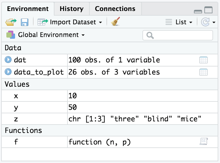
The ls function displays the names of objects in your workspace:
x<-10y<-50z<-c("three","blind","mice")f<-function(n,p)sqrt(p*(1-p)/n)ls()#> [1] "f" "x" "y" "z"
Notice that ls returns a vector of character strings in which each
string is the name of one variable or function. When your workspace is
empty, ls returns an empty vector, which produces this puzzling
output:
ls()#> character(0)
That is R’s quaint way of saying that ls returned a zero-length vector
of strings; that is, it returned an empty vector because nothing is
defined in your workspace.
If you want more than just a list of names, try ls.str; this will also
tell you something about each variable:
x<-10y<-50z<-c("three","blind","mice")f<-function(n,p)sqrt(p*(1-p)/n)ls.str()#> f : function (n, p)#> x : num 10#> y : num 50#> z : chr [1:3] "three" "blind" "mice"
The function is called ls.str because it is both listing your
variables and applying the str function to them, showing their
structure (Revealing the Structure of an Object).
Ordinarily, ls does not return any name that begins with a dot (.).
Such names are considered hidden and are not normally of interest to
users. (This mirrors the Unix convention of not listing files whose
names begin with dot.) You can force ls to list everything by setting
the all.names argument to TRUE:
ls()#> [1] "f" "x" "y" "z"ls(all.names=TRUE)#> [1] ".Random.seed" "f" "x" "y"#> [5] "z"
See “Deleting Variables” for deleting variables and Recipe X-X for inspecting your variables.
You want to remove unneeded variables or functions from your workspace or to erase its contents completely.
Use the rm function.
Your workspace can get cluttered quickly. The rm function removes,
permanently, one or more objects from the workspace:
x<-2*pix#> [1] 6.28rm(x)x#> Error in eval(expr, envir, enclos): object 'x' not found
There is no “undo”; once the variable is gone, it’s gone.
You can remove several variables at once:
rm(x,y,z)
You can even erase your entire workspace at once. The rm function has
a list argument consisting of a vector of names of variables to
remove. Recall that the ls function returns a vector of variables
names; hence you can combine rm and ls to erase everything:
ls()#> [1] "f" "x" "y" "z"rm(list=ls())ls()#> character(0)
Alternativly you could click the broom icon in the top of the Environment pane in R Studio, shown in Figure 2-1.
Never put rm(list=ls()) into code you share with others, such as a
library function or sample code sent to a mailing list or Stack
Overflow. Deleting all the variables in someone else’s workspace is
worse than rude and will make you extremely unpopular.
See “Listing Variables”.
You want to create a vector.
Use the c(...) operator to construct a vector from given values.
Vectors are a central component of R, not just another data structure. A vector can contain either numbers, strings, or logical values but not a mixture.
The c(...) operator can construct a vector from simple elements:
c(1,1,2,3,5,8,13,21)#> [1] 1 1 2 3 5 8 13 21c(1*pi,2*pi,3*pi,4*pi)#> [1] 3.14 6.28 9.42 12.57c("My","twitter","handle","is","@cmastication")#> [1] "My" "twitter" "handle" "is"#> [5] "@cmastication"c(TRUE,TRUE,FALSE,TRUE)#> [1] TRUE TRUE FALSE TRUE
If the arguments to c(...) are themselves vectors, it flattens them
and combines them into one single vector:
v1<-c(1,2,3)v2<-c(4,5,6)c(v1,v2)#> [1] 1 2 3 4 5 6
Vectors cannot contain a mix of data types, such as numbers and strings. If you create a vector from mixed elements, R will try to accommodate you by converting one of them:
v1<-c(1,2,3)v3<-c("A","B","C")c(v1,v3)#> [1] "1" "2" "3" "A" "B" "C"
Here, the user tried to create a vector from both numbers and strings. R converted all the numbers to strings before creating the vector, thereby making the data elements compatible. Note that R does this without warning or complaint.
Technically speaking, two data elements can coexist in a vector only if
they have the same mode. The modes of 3.1415 and "foo" are numeric
and character, respectively:
mode(3.1415)#> [1] "numeric"mode("foo")#> [1] "character"
Those modes are incompatible. To make a vector from them, R converts
3.1415 to character mode so it will be compatible with "foo":
c(3.1415,"foo")#> [1] "3.1415" "foo"mode(c(3.1415,"foo"))#> [1] "character"
c is a generic operator, which means that it works with many datatypes
and not just vectors. However, it might not do exactly what you expect,
so check its behavior before applying it to other datatypes and objects.
See the “Introduction” to the Chapter 5 chapter for more about vectors and other data structures.
You want to calculate basic statistics: mean, median, standard deviation, variance, correlation, or covariance.
Use one of these functions as applies, assuming that x and y are
vectors:
mean(x)
median(x)
sd(x)
var(x)
cor(x, y)
cov(x, y)
When you first use R you might open the docuentation and begin searching for material entitled “Procedures for Calculating Standard Deviation.” It seems that such an important topic would likely require a whole chapter.
It’s not that complicated.
Standard deviation and other basic statistics are calculated by simple functions. Ordinarily, the function argument is a vector of numbers and the function returns the calculated statistic:
x<-c(0,1,1,2,3,5,8,13,21,34)mean(x)#> [1] 8.8median(x)#> [1] 4sd(x)#> [1] 11var(x)#> [1] 122
The sd function calculates the sample standard deviation, and var
calculates the sample variance.
The cor and cov functions can calculate the correlation and
covariance, respectively, between two vectors:
x<-c(0,1,1,2,3,5,8,13,21,34)y<-log(x+1)cor(x,y)#> [1] 0.907cov(x,y)#> [1] 11.5
All these functions are picky about values that are not available (NA). Even one NA value in the vector argument causes any of these functions to return NA or even halt altogether with a cryptic error:
x<-c(0,1,1,2,3,NA)mean(x)#> [1] NAsd(x)#> [1] NA
It’s annoying when R is that cautious, but it is the right thing to do.
You must think carefully about your situation. Does an NA in your data
invalidate the statistic? If yes, then R is doing the right thing. If
not, you can override this behavior by setting na.rm=TRUE, which tells
R to ignore the NA values:
x<-c(0,1,1,2,3,NA)sd(x,na.rm=TRUE)#> [1] 1.14
In older versions of R, mean and sd were smart about data frames.
They understood that each column of the data frame is a different
variable, so they calculated their statistic for each column
individually. This is no longer the case and, as a result, you may read
confusing comments online or in older books (like version 1 of this
book). In order to apply the functions to each column of a dataframe we
now need to use a helper function. The Tidyverse family of helper
functions for this sort of thing are in the purrr package. As with
other Tidyverse packages, this gets loaded when you run
library(tidyverse). The function we’ll use to apply a function to each
column of a data frame is map_dbl:
data(cars)map_dbl(cars,mean)#> speed dist#> 15.4 43.0map_dbl(cars,sd)#> speed dist#> 5.29 25.77map_dbl(cars,median)#> speed dist#> 15 36
Notice that using map_dbl to apply mean or sd each return two
values, one for each column defined by the data frame. (Technically,
they return a two-element vector whose names attribute is taken from
the columns of the data frame.)
The var function understands data frames without the help of a mapping
function. It calculates the covariance between the columns of the data
frame and returns the covariance matrix:
var(cars)#> speed dist#> speed 28 110#> dist 110 664
Likewise, if x is either a data frame or a matrix, then cor(x)
returns the correlation matrix and cov(x) returns the covariance
matrix:
cor(cars)#> speed dist#> speed 1.000 0.807#> dist 0.807 1.000cov(cars)#> speed dist#> speed 28 110#> dist 110 664
See Recipes:
“Avoiding Some Common Mistakes”
“Merging Data Frames by Common Column”
Recipe X-X
You want to create a sequence of numbers.
Use an n:m expression to create the simple sequence n, n+1, n+2,
…, m:
1:5#> [1] 1 2 3 4 5
Use the seq function for sequences with an increment other than 1:
seq(from=1,to=5,by=2)#> [1] 1 3 5
Use the rep function to create a series of repeated values:
rep(1,times=5)#> [1] 1 1 1 1 1
The colon operator (n:m) creates a vector containing the sequence n,
n+1, n+2, …, m:
0:9#> [1] 0 1 2 3 4 5 6 7 8 910:19#> [1] 10 11 12 13 14 15 16 17 18 199:0#> [1] 9 8 7 6 5 4 3 2 1 0
Observe that R was clever with the last expression (9:0). Because 9 is
larger than 0, it counts backward from the starting to ending value. You
can also use the colon operator directly with the pipe to pass data to
another function:
10:20%>%mean()
The colon operator works for sequences that grow by 1 only. The seq
function also builds sequences but supports an optional third argument,
which is the increment:
seq(from=0,to=20)#> [1] 0 1 2 3 4 5 6 7 8 9 10 11 12 13 14 15 16 17 18 19 20seq(from=0,to=20,by=2)#> [1] 0 2 4 6 8 10 12 14 16 18 20seq(from=0,to=20,by=5)#> [1] 0 5 10 15 20
Alternatively, you can specify a length for the output sequence and then R will calculate the necessary increment:
seq(from=0,to=20,length.out=5)#> [1] 0 5 10 15 20seq(from=0,to=100,length.out=5)#> [1] 0 25 50 75 100
The increment need not be an integer. R can create sequences with fractional increments, too:
seq(from=1.0,to=2.0,length.out=5)#> [1] 1.00 1.25 1.50 1.75 2.00
For the special case of a “sequence” that is simply a repeated value you
should use the rep function, which repeats its first argument:
rep(pi,times=5)#> [1] 3.14 3.14 3.14 3.14 3.14
See “Creating a Sequence of Dates” for creating a sequence of Date objects.
You want to compare two vectors or you want to compare an entire vector against a scalar.
The comparison operators (==, !=, <, >, <=, >=) can perform
an element-by-element comparison of two vectors. They can also compare a
vector’s element against a scalar. The result is a vector of logical
values in which each value is the result of one element-wise comparison.
R has two logical values, TRUE and FALSE. These are often called
Boolean values in other programming languages.
The comparison operators compare two values and return TRUE or
FALSE, depending upon the result of the comparison:
a<-3a==pi# Test for equality#> [1] FALSEa!=pi# Test for inequality#> [1] TRUEa<pi#> [1] TRUEa>pi#> [1] FALSEa<=pi#> [1] TRUEa>=pi#> [1] FALSE
You can experience the power of R by comparing entire vectors at once. R will perform an element-by-element comparison and return a vector of logical values, one for each comparison:
v<-c(3,pi,4)w<-c(pi,pi,pi)v==w# Compare two 3-element vectors#> [1] FALSE TRUE FALSEv!=w#> [1] TRUE FALSE TRUEv<w#> [1] TRUE FALSE FALSEv<=w#> [1] TRUE TRUE FALSEv>w#> [1] FALSE FALSE TRUEv>=w#> [1] FALSE TRUE TRUE
You can also compare a vector against a single scalar, in which case R will expand the scalar to the vector’s length and then perform the element-wise comparison. The previous example can be simplified in this way:
v<-c(3,pi,4)v==pi# Compare a 3-element vector against one number#> [1] FALSE TRUE FALSEv!=pi#> [1] TRUE FALSE TRUE
(This is an application of the Recycling Rule, “Understanding the Recycling Rule”.)
After comparing two vectors, you often want to know whether any of the
comparisons were true or whether all the comparisons were true. The
any and all functions handle those tests. They both test a logical
vector. The any function returns TRUE if any element of the vector
is TRUE. The all function returns TRUE if all elements of the
vector are TRUE:
v<-c(3,pi,4)any(v==pi)# Return TRUE if any element of v equals pi#> [1] TRUEall(v==0)# Return TRUE if all elements of v are zero#> [1] FALSE
You want to extract one or more elements from a vector.
Select the indexing technique appropriate for your problem:
Use square brackets to select vector elements by their position, such
as v[3] for the third element of v.
Use negative indexes to exclude elements.
Use a vector of indexes to select multiple values.
Use a logical vector to select elements based on a condition.
Use names to access named elements.
Selecting elements from vectors is another powerful feature of R. Basic selection is handled just as in many other programming languages—use square brackets and a simple index:
fib<-c(0,1,1,2,3,5,8,13,21,34)fib#> [1] 0 1 1 2 3 5 8 13 21 34fib[1]#> [1] 0fib[2]#> [1] 1fib[3]#> [1] 1fib[4]#> [1] 2fib[5]#> [1] 3
Notice that the first element has an index of 1, not 0 as in some other programming languages.
A cool feature of vector indexing is that you can select multiple elements at once. The index itself can be a vector, and each element of that indexing vector selects an element from the data vector:
fib[1:3]# Select elements 1 through 3#> [1] 0 1 1fib[4:9]# Select elements 4 through 9#> [1] 2 3 5 8 13 21
An index of 1:3 means select elements 1, 2, and 3, as just shown. The indexing vector needn’t be a simple sequence, however. You can select elements anywhere within the data vector—as in this example, which selects elements 1, 2, 4, and 8:
fib[c(1,2,4,8)]#> [1] 0 1 2 13
R interprets negative indexes to mean exclude a value. An index of −1, for instance, means exclude the first value and return all other values:
fib[-1]# Ignore first element#> [1] 1 1 2 3 5 8 13 21 34
This method can be extended to exclude whole slices by using an indexing vector of negative indexes:
fib[1:3]# As before#> [1] 0 1 1fib[-(1:3)]# Invert sign of index to exclude instead of select#> [1] 2 3 5 8 13 21 34
Another indexing technique uses a logical vector to select elements from
the data vector. Everywhere that the logical vector is TRUE, an
element is selected:
fib<10# This vector is TRUE wherever fib is less than 10#> [1] TRUE TRUE TRUE TRUE TRUE TRUE TRUE FALSE FALSE FALSEfib[fib<10]# Use that vector to select elements less than 10#> [1] 0 1 1 2 3 5 8fib%%2==0# This vector is TRUE wherever fib is even#> [1] TRUE FALSE FALSE TRUE FALSE FALSE TRUE FALSE FALSE TRUEfib[fib%%2==0]# Use that vector to select the even elements#> [1] 0 2 8 34
Ordinarily, the logical vector should be the same length as the data vector so you are clearly either including or excluding each element. (If the lengths differ then you need to understand the Recycling Rule, “Understanding the Recycling Rule”.)
By combining vector comparisons, logical operators, and vector indexing, you can perform powerful selections with very little R code:
Select all elements greater than the median
v<-c(3,6,1,9,11,16,0,3,1,45,2,8,9,6,-4)v[v>median(v)]#> [1] 9 11 16 45 8 9
Select all elements in the lower and upper 5%
v[(v<quantile(v,0.05))|(v>quantile(v,0.95))]#> [1] 45 -4
The above example uses the | operator which means “or” when indexing.
If you wanted “and” you use the & operator.
Select all elements that exceed ±1 standard deviations from the mean
v[abs(v-mean(v))>sd(v)]#> [1] 45 -4
Select all elements that are neither NA nor NULL
v<-c(1,2,3,NA,5)v[!is.na(v)&!is.null(v)]#> [1] 1 2 3 5
One final indexing feature lets you select elements by name. It assumes
that the vector has a names attribute, defining a name for each
element. This can be done by assigning a vector of character strings to
the attribute:
years<-c(1960,1964,1976,1994)names(years)<-c("Kennedy","Johnson","Carter","Clinton")years#> Kennedy Johnson Carter Clinton#> 1960 1964 1976 1994
Once the names are defined, you can refer to individual elements by name:
years["Carter"]#> Carter#> 1976years["Clinton"]#> Clinton#> 1994
This generalizes to allow indexing by vectors of names: R returns every element named in the index:
years[c("Carter","Clinton")]#> Carter Clinton#> 1976 1994
See “Understanding the Recycling Rule” for more about the Recycling Rule.
You want to operate on an entire vector at once.
The usual arithmetic operators can perform element-wise operations on entire vectors. Many functions operate on entire vectors, too, and return a vector result.
Vector operations are one of R’s great strengths. All the basic arithmetic operators can be applied to pairs of vectors. They operate in an element-wise manner; that is, the operator is applied to corresponding elements from both vectors:
v<-c(11,12,13,14,15)w<-c(1,2,3,4,5)v+w#> [1] 12 14 16 18 20v-w#> [1] 10 10 10 10 10v*w#> [1] 11 24 39 56 75v/w#> [1] 11.00 6.00 4.33 3.50 3.00w^v#> [1] 1.00e+00 4.10e+03 1.59e+06 2.68e+08 3.05e+10
Observe that the length of the result here is equal to the length of the original vectors. The reason is that each element comes from a pair of corresponding values in the input vectors.
If one operand is a vector and the other is a scalar, then the operation is performed between every vector element and the scalar:
w#> [1] 1 2 3 4 5w+2#> [1] 3 4 5 6 7w-2#> [1] -1 0 1 2 3w*2#> [1] 2 4 6 8 10w/2#> [1] 0.5 1.0 1.5 2.0 2.52^w#> [1] 2 4 8 16 32
For example, you can recenter an entire vector in one expression simply by subtracting the mean of its contents:
w#> [1] 1 2 3 4 5mean(w)#> [1] 3w-mean(w)#> [1] -2 -1 0 1 2
Likewise, you can calculate the z-score of a vector in one expression: subtract the mean and divide by the standard deviation:
w#> [1] 1 2 3 4 5sd(w)#> [1] 1.58(w-mean(w))/sd(w)#> [1] -1.265 -0.632 0.000 0.632 1.265
Yet the implementation of vector-level operations goes far beyond
elementary arithmetic. It pervades the language, and many functions
operate on entire vectors. The functions sqrt and log, for example,
apply themselves to every element of a vector and return a vector of
results:
w<-1:5w#> [1] 1 2 3 4 5sqrt(w)#> [1] 1.00 1.41 1.73 2.00 2.24log(w)#> [1] 0.000 0.693 1.099 1.386 1.609sin(w)#> [1] 0.841 0.909 0.141 -0.757 -0.959
There are two great advantages to vector operations. The first and most obvious is convenience. Operations that require looping in other languages are one-liners in R. The second is speed. Most vectorized operations are implemented directly in C code, so they are substantially faster than the equivalent R code you could write.
Performing an operation between a vector and a scalar is actually a special case of the Recycling Rule; see “Understanding the Recycling Rule”.
Your R expression is producing a curious result, and you wonder if operator precedence is causing problems.
The full list of operators is shown in table @ref(tab:precedence), listed in order of precedence from highest to lowest. Operators of equal precedence are evaluated from left to right except where indicated.
| Operator | Meaning | See also |
|---|---|---|
|
Indexing |
|
|
Access variables in a name space (environment) |
|
|
Component extraction, slot extraction |
|
|
Exponentiation (right to left) |
|
|
Unary minus and plus |
|
|
Sequence creation |
Recipes pass:[<a data-type="xref” data-xrefstyle="select:labelnumber” href="#recipe-id021">#recipe-id021</a>, <a data-type="xref” data-xrefstyle="select:labelnumber” href="#recipe-id047">#recipe-id047</a> |
|
g |
Discussion |
|
Multiplication, division |
Discussion |
|
Addition, subtraction |
|
|
Comparison |
|
|
Logical negation |
|
|
Logical “and”, short-circuit “and” |
|
` |
||
` |
Logical “or”, short-circuit “or” |
|
|
Formula |
|
|
Rightward assignment |
|
|
Assignment (right to left) |
|
|
Assignment (right to left) |
|
|
Help |
It’s not important that you know what every one of these operators do, or what they mean. The list here is to expose you to the idea that different operators have different precedence.
Getting your operator precedence wrong in R is a common problem. It
certainly happens to the authors a lot. We unthinkingly expect that the
expression 0:n−1 will create a sequence of integers from 0 to n − 1
but it does not:
n<-100:n-1#> [1] -1 0 1 2 3 4 5 6 7 8 9
It creates the sequence from −1 to n − 1 because R interprets it as
(0:n)−1.
You might not recognize the notation %`_any_%` in the table. R
interprets any text between percent signs (%…%) as a binary
operator. Several such operators have predefined meanings:
%%Modulo operator
%/%Integer division
%*%Matrix multiplication
%in%Returns TRUE if the left operand occurs in its right operand;
FALSE otherwise
%>%Pipe that passes results from the left to a function on the right
You can also define new binary operators using the %…% notation;
see Defining Your Own Binary Operators. The point
here is that all such operators have the same precedence.
See “Performing Vector Arithmetic” for more about vector operations, “Performing Matrix Operations” for more about matrix operations, and Recipe X-X to define your own operators. See the Arithmetic and Syntax topics in the R help pages as well as Chapters 5 and 6 of R in a Nutshell (O’Reilly).
You are getting tired of typing long sequences of commands and especially tired of typing the same ones over and over.
Open an editor window and accumulate your reusable blocks of R commands there. Then, execute those blocks directly from that window. Reserve the command line for typing brief or one-off commands.
When you are done, you can save the accumulated code blocks in a script file for later use.
The typical beginner to R types an expression in the console window and sees what happens. As he gets more comfortable, he types increasingly complicated expressions. Then he begins typing multiline expressions. Soon, he is typing the same multiline expressions over and over, perhaps with small variations, in order to perform his increasingly complicated calculations.
The experienced user does not often retype a complex expression. She may type the same expression once or twice, but when she realizes it is useful and reusable she will cut-and-paste it into an editor window. To execute the snippet thereafter, she selects the snippet in the editor window and tells R to execute it, rather than retyping it. This technique is especially powerful as her snippets evolve into long blocks of code.
In R Studio, a few features of the IDE facilitate this workstyle. Windows and Linux machines have slightly different keys than Mac machines: Windows/Linux uses the Ctrl and Alt modifiers, whereas the Mac uses Cmd and Opt.
From the main menu, select File → New File then select the type of file you want to create, in this case, an R Script.
Position the cursor on the line and then press Ctrl+Enter (Windows) or Cmd+Enter (Mac) to execute it.
Highlight the lines using your mouse; then press Ctrl+Enter (Windows) or Cmd+Enter (Mac) to execute them.
Press Ctrl+Alt+R (Windows) or Cmd+Opt+R (Mac) to execute the whole
editor window. Or from the menu click Code → Run Region →
Run All
These keyboard shortcuts and dozens more can be found within R Studio by
clicking the menu: Tools → Keyboard Shortcuts Help
Copying lines from the console window to the editor window is simply a matter of copy and paste. When you exit R Studio, it will ask if you want to save the new script. You can either save it for future reuse or discard it.
Creating many intermediate variables in your code is tedious and overly verbose, while nesting R functions seems nearly unreadable.
Use the pipe operator (%>%) to make your expression easier to read and
write. The pipe operator (%>%), created by Stefan Bache and found in
the magrittr package and used extensivly in many tidyverse functions
as well.
Us the pipe operator to combine multiple functions together into a “pipeline” of functions without intermediate variables:
library(tidyverse)data(mpg)mpg%>%filter(cty>21)%>%head(3)%>%()#> # A tibble: 3 x 11#> manufacturer model displ year cyl trans drv cty hwy fl class#> <chr> <chr> <dbl> <int> <int> <chr> <chr> <int> <int> <chr> <chr>#> 1 chevrolet mali~ 2.4 2008 4 auto~ f 22 30 r mids~#> 2 honda civic 1.6 1999 4 manu~ f 28 33 r subc~#> 3 honda civic 1.6 1999 4 auto~ f 24 32 r subc~
The pipe is much cleaner and easier to read than using intermediate temporary variables:
temp1<-filter(mpg,cty>21)temp2<-head(temp1,3)(temp2)#> # A tibble: 3 x 11#> manufacturer model displ year cyl trans drv cty hwy fl class#> <chr> <chr> <dbl> <int> <int> <chr> <chr> <int> <int> <chr> <chr>#> 1 chevrolet mali~ 2.4 2008 4 auto~ f 22 30 r mids~#> 2 honda civic 1.6 1999 4 manu~ f 28 33 r subc~#> 3 honda civic 1.6 1999 4 auto~ f 24 32 r subc~
The pipe operator does not provide any new functionality to R, but it can greatly improve readability of code. The pipe operator takes the output of the function or object on the left of the operator and passes it as the first argument of the function on the right.
Writing this:
x%>%head()
is functionally the same as writing this:
head(x)
In both cases x is the argument to head. We can supply additional
arguments, but x is always the first argument. These two lines are
functionally identical:
x%>%head(n=10)head(x,n=10)
This difference may seem small, but with a more complicated example, the
benefits begin to accumulate. If we had a workflow where we wanted to
use filter to limit our data to values, then select to keep only
certain variables, followed by ggplot to create a simple plot, we
could use intermediate variables.
library(tidyverse)filtered_mpg<-filter(mpg,cty>21)selected_mpg<-select(filtered_mpg,cty,hwy)ggplot(selected_mpg,aes(cty,hwy))+geom_point()
This incremental approach is fairly readable but creates a number of intermediate data frames and requires the user to keep track of the state of many objects which can generate a cognitive load on the user.
Another alternative is to nest the functions together:
ggplot(select(filter(mpg,cty>21),cty,hwy),aes(cty,hwy))+geom_point()
While this is very concise since it’s only one line, this code requires much more attention to read and understand what’s going on. Code that is difficult for the user to parse mentally can introduce potential for error, and also make maintenance of the code harder in the future.
mpg%>%filter(cty>21)%>%select(cty,hwy)%>%ggplot(aes(cty,hwy))+geom_point()
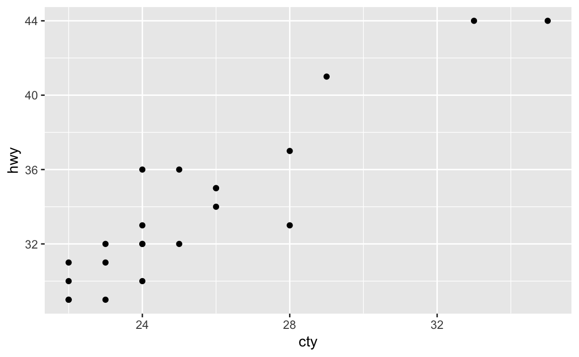
The above code starts with the mpg dataset, pipes it to the filter
function which keeps only records where the city mpg (cty) is greater
than 21. Those results are piped into the select command that keeps
only the listed variables cty and hwy and those are piped into the
ggplot command where an point plot is produced in Figure 2-2
If you want the argument going into your target (right hand side)
function to be somewhere other than the first argument, use the dot
(.) operator:
iris%>%head(3)
is the same as:
iris%>%head(3,x=.)
However in the second example we passed the iris data frame into the second named argument using the dot operator. This can be handy for functions where the input data frame goes in a position other than the first argument.
Through this book we use pipes to hold together data transformations with multiple steps. We typically format the code with a line break after each pipe and then we indent the code on the following lines. This makes the code easily identifiable as parts of the same data pipeline.
You want to avoid some of the common mistakes made by beginning users—and also by experienced users, for that matter.
Here are some easy ways to make trouble for yourself:
Forgetting the parentheses after a function invocation:
You call an R function by putting parentheses after the name. For
instance, this line invokes the ls function:
ls()
However, if you omit the parentheses then R does not execute the function. Instead, it shows the function definition, which is almost never what you want:
ls# > function (name, pos = -1L, envir = as.environment(pos), all.names = FALSE,# > pattern, sorted = TRUE)# > {# > if (!missing(name)) {# > pos <- tryCatch(name, error = function(e) e)# > if (inherits(pos, "error")) {# > name <- substitute(name)# > if (!is.character(name))# > name <- deparse(name)# > etc...
Forgetting to double up backslashes in Windows file paths
This function call appears to read a Windows file called
F:\research\bio\assay.csv, but it does not:
tbl<-read.csv("F:\research\bio\assay.csv")
Backslashes (\) inside character strings have a special meaning and
therefore need to be doubled up. R will interpret this file name as
F:researchbioassay.csv, for example, which is not what the user
wanted. See “Dealing with “Cannot Open File” in Windows” for possible solutions.
Mistyping “<-” as “< (blank) -”
The assignment operator is <-, with no space between the < and the
-:
x<-pi# Set x to 3.1415926...
If you accidentally insert a space between < and -, the meaning
changes completely:
x<-pi# Oops! We are comparing x instead of setting it!#> [1] FALSE
This is now a comparison (<) between x and negative π (-pi). It
does not change x. If you are lucky, x is undefined and R will
complain, alerting you that something is fishy:
x<-pi#> Error in eval(expr, envir, enclos): object 'x' not found
If x is defined, R will perform the comparison and print a logical
value, TRUE or FALSE. That should alert you that something is wrong:
an assignment does not normally print anything:
x<-0# Initialize x to zerox<-pi# Oops!#> [1] FALSE
Incorrectly continuing an expression across lines
R reads your typing until you finish a complete expression, no matter
how many lines of input that requires. It prompts you for additional
input using the + prompt until it is satisfied. This example splits an
expression across two lines:
total<-1+2+3+# Continued on the next line4+5(total)#> [1] 15
Problems begin when you accidentally finish the expression prematurely, which can easily happen:
total<-1+2+3# Oops! R sees a complete expression+4+5# This is a new expression; R prints its value#> [1] 9(total)#> [1] 6
There are two clues that something is amiss: R prompted you with a
normal prompt (>), not the continuation prompt (+); and it printed
the value of 4 + 5.
This common mistake is a headache for the casual user. It is a nightmare for programmers, however, because it can introduce hard-to-find bugs into R scripts.
Using = instead of ==
Use the double-equal operator (==) for comparisons. If you
accidentally use the single-equal operator (=), you will irreversibly
overwrite your variable:
v<-1# Assign 1 to vv==0# Compare v against zero#> [1] FALSEv<-0# Assign 0 to v, overwriting previous contents
Writing 1:n+1 when you mean 1:(n+1)
You might think that 1:n+1 is the sequence of numbers 1, 2, …, n,
n + 1. It’s not. It is the sequence 1, 2, …, n with 1 added to
every element, giving 2, 3, …, n, n + 1. This happens because R
interprets 1:n+1 as (1:n)+1. Use parentheses to get exactly what you
want:
n<-51:n+1#> [1] 2 3 4 5 61:(n+1)#> [1] 1 2 3 4 5 6
Getting bitten by the Recycling Rule
Vector arithmetic and vector comparisons work well when both vectors
have the same length. However, the results can be baffling when the
operands are vectors of differing lengths. Guard against this
possibility by understanding and remembering the Recycling Rule,
“Understanding the Recycling Rule”.
Installing a package but not loading it with library() or
require()
Installing a package is the first step toward using it, but one more
step is required. Use library or require to load the package into
your search path. Until you do so, R will not recognize the functions or
datasets in the package. See “Accessing the Functions in a Package”:
x<-rnorm(100)n<-5truehist(x,n)#> Error in truehist(x, n): could not find function "truehist"
However if we load the library first, then the code runs and we get the chart shown in Figure 2-3.
library(MASS)# Load the MASS package into Rtruehist(x,n)
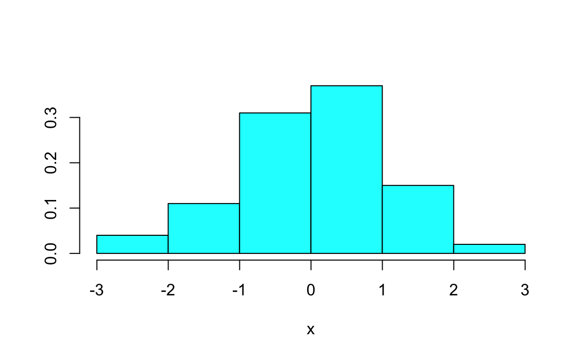
We typically use library() instead of require(). The reason is that
if you create an R script that uses library() and the desired package
is not already installed, R will return an error. While require(), in
contrast, will simply return FALSE if the package is not installed.
Writing aList[i] when you mean aList[[i]], or vice versa
If the variable lst contains a list, it can be indexed in two ways:
lst[[n]] is the _n_th element of the list; whereas lst[n] is a list
whose only element is the _n_th element of lst. That’s a big
difference. See “Selecting List Elements by Position”.
Using & instead of &&, or vice versa; same for | and ||
Use & and | in logical expressions involving the logical values
TRUE and FALSE. See “Selecting Vector Elements”.
Use && and || for the flow-of-control expressions inside if and
while statements.
Programmers accustomed to other programming languages may reflexively
use && and || everywhere because “they are faster.” But those
operators give peculiar results when applied to vectors of logical
values, so avoid them unless you are sure that they do what you want.
Passing multiple arguments to a single-argument function
What do you think is the value of mean(9,10,11)? No, it’s not 10. It’s
9. The mean function computes the mean of the first argument. The
second and third arguments are being interpreted as other, positional
arguments. To pass multiple items into a single argument, we put them in
a vector with the c operator. mean(c(9,10,11)) will return 10, as
you might expect.
Some functions, such as mean, take one argument. Other arguments, such
as max and min, take multiple arguments and apply themselves across
all arguments. Be sure you know which is which.
Thinking that max behaves like pmax, or that min behaves like
pmin
The max and min functions have multiple arguments and return one
value: the maximum or minimum of all their arguments.
The pmax and pmin functions have multiple arguments but return a
vector with values taken element-wise from the arguments. See
Finding Parwise Minimums or Maximums.
Misusing a function that does not understand data frames
Some functions are quite clever regarding data frames. They apply
themselves to the individual columns of the data frame, computing their
result for each individual column. Sadly, not all functions are that
clever. This includes the mean, median, max, and min functions.
They will lump together every value from every column and compute their
result from the lump or possibly just return an error. Be aware of which
functions are savvy to data frames and which are not.
Using single backslash (\) in Windows Paths If you are using R on
Windows, it is common to copy and paste a file path into your R script.
Windows File Explorer will show you that your path is
C:\temp\my_file.csv but if you try to tell R to read that file, you’ll
get a cryptic message:
Error: '\m' is an unrecognized escape in character string starting "'.\temp\m"
This is because R sees backslashes as special characters. You can get
around this either by using forward slashes (/), or using double
backslashes, (\\).
read_csv(`./temp/my_file.csv`)read_csv(`.\\temp\\my_file.csv`)
This is only an issue on Windows because both Mac and Linux use forward slashes as path seperators.
Posting a question to Stack Overflow or the mailing list before
searching for the answer
Don’t waste your time. Don’t waste other people’s time. Before you post
a question to a mailing list or to Stack Overflow, do your homework and
search the archives. Odds are, someone has already answered your
question. If so, you’ll see the answer in the discussion thread for the
question. See “Searching the Mailing Lists”.
You want to change your working directory. Or you just want to know what it is.
Navigate to a directory in the file pane. Then from the File Pane, select More → Set as Working Directory as shown in Figure 3-1.
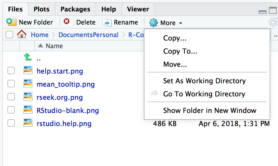
Use getwd to report the working directory, and use setwd to change
it:
getwd()#> [1] "/Users/jal/DocumentsPersonal/R-Cookbook"
setwd("~/Documents/MyDirectory")
Your working directory is important because it is the default location for all file input and output—including reading and writing data files, opening and saving script files, and saving your workspace image. When you open a file and do not specify an absolute path, R will assume that the file is in your working directory.
If you’re using R Studio projects, your default working directory will be the home directory of the project. See “Creating a new R Studio Project” for more about creating R Studio Projects.
See “Dealing with “Cannot Open File” in Windows” for dealing with filenames in Windows.
You want to create a new R Studio Project to keep all your files related to a specific project.
Projects are a powerful concept that’s specific to R Studio. Projects set your working directory to the project directory but they add considerable additional help to maintaining your project.
Projects help you by doing the following:
Sets your working directory to the project directory
Preserves window state in R Studio so when you return to a project your windows are all as you left them. This includes opening any files you had open when you last saved your project.
Preserves R Studio Project settings
To hold your project settings, R Studio will create a project file with an .Rproj extension in the project directory. The project file contains your project settings and if you open the project file in R Studio it works like a shortcut for opening the project. In addition, R Studio creates a hidden directory named .Rporj.user to house temporary files related to your project.
We recommend that any time you work in R that is non trivial you should create an R Studio Project. Projects help you keep organized and make workflow on your projects easier.
You want to save your workspace from the console or within a program.
Call the save.image function:
save.image()
Your workspace holds your R variables and functions, and it is created
when R starts. The workspace is held in your computer’s main memory and
lasts until you exit from R, at which time you can save it. The contents
of your workspace can be easily seen in R Studio in the Environment
tab shown in Figure 2-1
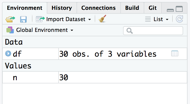
However, you may want to save your workspace without exiting R. Becuase
you know bad things mysteriously happen when you close your laptop to
carry it home. Use the save.image function.
The workspace is written to a file called .RData in the working
directory. When R starts, it looks for that file and, if found,
initializes the workspace from it.
A sad fact is that the workspace does not include your open graphs: that cool graph on your screen disappears when you exit R. The workspace also does not include saving the position of your windows or your R Studio settings. This is why we recommend using R Studio projects as a project includes your workspace and a whole lot more.
See “Installing R Studio” for how to save your workspace when exiting R and “Getting and Setting the Working Directory” for setting the working directory.
You want to see your recent sequence of commands.
Depending on what you are trying to accomplish, you can use a few different methods to access prior command history. If you are in the Console you can press the up arrow to interactively scroll through past commands.
If you want to see a listing of past commands, you can either execute
the history function, or the History window in R Studio to view your
most recent input:
history()
In R Studio typing history() into the Console simply activates the
History pane in R Studio (Figure 3-2). You could also make
that pane visable by clicking on it with your cursor.
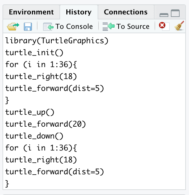
The history function will display your most recent commands. In R
Studio the history command will activate the History window. If you
were running R outside of R Studio, history shows the most recent 25
lines, but you can request more:
history(100)# Show 100 most recent lines of historyhistory(Inf)# Show entire saved history
From within R Studio, the History tab shows an exhaustive list of past commands in chronological order with the most recent at the bottom of the list. In R Studio you can highlight past commands with your cursor then click on the “To Console” or “To Source” to copy past commands into the console or source editor, respectively. This can be terribly handy when you’ve done interactive data analysis and then decide you want to save some past steps to a source file for later use.
From the console you can see your history by simply scrolling backward through your input by pressing the up arrow causing your previous typing to reappear, one line at a time.
If you’ve exited from R or R Studio then you can still see your command
history. It saves the history in a file called .Rhistory in the
working directory. Open the file with a text editor and then scroll to
the bottom; you will see your most recent typing.
You typed an expression into R that calculated the value, but you forgot to save the result in a variable.
A special variable called .Last.value saves the value of the most
recently evaluated expression. Save it to a variable before you type
anything else.
It is frustrating to type a long expression or call a long-running
function but then forget to save the result. Fortunately, you needn’t
retype the expression nor invoke the function again—the result was saved
in the .Last.value variable:
aVeryLongRunningFunction()# Oops! Forgot to save the result!x<-.Last.value# Capture the result now
A word of caution: the contents of .Last.value are overwritten every
time you type another expression, so capture the value immediately. If
you don’t remember until another expression has been evaluated, it’s too
late!
See “Viewing Your Command History” to recall your command history.
You want to see the list of packages currently loaded into R.
Use the search function with no arguments:
search()
The search path is a list of packages that are currently loaded into memory and available for use. Although many packages may be installed on your computer, only a few of them are actually loaded into the R interpreter at any given moment. You might be wondering which packages are loaded right now.
With no arguments, the search function returns the list of loaded
packages. It produces an output like this:
search()#> [1] ".GlobalEnv" "package:knitr" "package:forcats"#> [4] "package:stringr" "package:dplyr" "package:purrr"#> [7] "package:readr" "package:tidyr" "package:tibble"#> [10] "package:ggplot2" "package:tidyverse" "package:stats"#> [13] "package:graphics" "package:grDevices" "package:utils"#> [16] "package:datasets" "package:methods" "Autoloads"#> [19] "package:base"
Your machine may return a different result, depending on what’s
installed there. The return value of search is a vector of strings.
The first string is ".GlobalEnv", which refers to your workspace. Most
strings have the form "package:packagename", which indicates that the
package called packagename is currently loaded into R. In the above
example, you can see many Tidyverse packages installed, including
purrr, ggplot2, tibble, etc.
R uses the search path to find functions. When you type a function name, R searches the path—in the order shown—until it finds the function in a loaded package. If the function is found, R executes it. Otherwise, it prints an error message and stops. (There is actually a bit more to it: the search path can contain environments, not just packages, and the search algorithm is different when initiated by an object within a package; see the R Language Definition for details.)
Since your workspace (.GlobalEnv) is first in the list, R looks for
functions in your workspace before searching any packages. If your
workspace and a package both contain a function with the same name, your
workspace will “mask” the function; this means that R stops searching
after it finds your function and so never sees the package function.
This is a blessing if you want to override the package function…and a
curse if you still want access to the package function. If you find
yourself feeling cursed because you (or some package you loaded)
overrode a function (or other object) from an existing loaded package,
you can use the full environment::name form to call an object from a
loaded package environment. For example, if you wanted to call the
dplyr function count you could do so using dplyr::count. Using the
full explicit name to call a function will work even if you have not
loaded the package. So if you have dplyr installed but not loaded, you
can still call dplyr::count. It is becoming increasingly common with
online examples to show the full packagename::function in examples.
While this removes ambiguity about where a function comes from, it makes
example code very wordy.
Note that R will only include loaded packages in the search path. So
if you have installed a package, but not loaded it by using
library(packagename) then R will not add that package to the search
path.
R also uses the search path to find R datasets (not files) or any other object via a similar procedure.
Unix & Mac users: don’t confuse the R search path with the Unix search
path (the PATH environment variable). They are conceptually similar
but two distinct things. The R search path is internal to R and is used
by R only to locate functions and datasets, whereas the Unix search path
is used by the OS to locate executable programs.
See “Accessing the Functions in a Package” for loading packages into R, “Viewing the List of Installed Packages” for the list of installed packages (not just loaded packages), and “Accessing Data Frame Contents More Easily” for inserting data frames into the search path.
A package installed on your computer is either a standard package or a package downloaded by you. When you try using functions in the package, however, R cannot find them.
Use either the library function or the require function to load the
package into R:
library(packagename)
R comes with several standard packages, but not all of them are
automatically loaded when you start R. Likewise, you can download and
install many useful packages from CRAN, or Github, but they are not
automatically loaded when you run R. The MASS package comes standard
with R, for example, but you could get this message when using the lda
function in that package:
lda(x)#> Error in lda(x): could not find function "lda"
R is complaining that it cannot find the lda function among the
packages currently loaded into memory.
When you use the library function or the require function, R loads
the package into memory and its contents become immediately available to
you:
my_model<-lda(cty~displ+year,data=mpg)#> Error in lda(cty ~ displ + year, data = mpg): could not find function "lda"library(MASS)# Load the MASS library into memory#>#> Attaching package: 'MASS'#> The following object is masked from 'package:dplyr':#>#> selectmy_model<-lda(cty~displ+year,data=mpg)# Now R can find the function
Before calling library, R does not recognize the function name.
Afterward, the package contents are available and calling the lda
function works.
Notice that you needn’t enclose the package name in quotes.
The require function is nearly identical to library. It has two
features that are useful for writing scripts. It returns TRUE if the
package was successfully loaded and FALSE otherwise. It also generates
a mere warning if the load fails—unlike library, which generates an
error.
Both functions have a key feature: they do not reload packages that are already loaded, so calling twice for the same package is harmless. This is especially nice for writing scripts. The script can load needed packages while knowing that loaded packages will not be reloaded.
The detach function will unload a package that is currently loaded:
detach(package:MASS)
Observe that the package name must be qualified, as in package:MASS.
One reason to unload a package is that it contains a function whose name conflicts with a same-named function lower on the search list. When such a conflict occurs, we say the higher function masks the lower function. You no longer “see” the lower function because R stops searching when it finds the higher function. Hence unloading the higher package unmasks the lower name.
You want to use one of R’s built-in datasets. Or you want to access one of the datasets that comes with another package.
The standard datasets distributed with R are already available to you,
since the datasets package is in your search path. If you’ve loaded
any other packages, datasets that come with those loaded packages will
also be availiable in your search path.
To access datasets in other packages, use the data function while
giving the dataset name and package name:
data(dsname,package="pkgname")
R comes with many built-in datasets. Other packages, such as dplyr and
ggplot2 also come with example data that’s used in the examples found
in their help files. These datasets are useful when you are learning
about R, since they provide data with which to experiment.
Many datasets are kept in a package called (naturally enough)
datasets, which is distributed with R. That package is in your search
path, so you have instant access to its contents. For example, you can
use the built-in dataset called pressure:
head(pressure)#> temperature pressure#> 1 0 0.0002#> 2 20 0.0012#> 3 40 0.0060#> 4 60 0.0300#> 5 80 0.0900#> 6 100 0.2700
If you want to know more about pressure, use the help function to
learn about it and other datasets:
help(pressure)# Bring up help page for pressure dataset
You can see a table of contents for datasets by calling the data
function with no arguments:
data()# Bring up a list of datasets
Any R package can elect to include datasets that supplement those
supplied in datasets. The MASS package, for example, includes many
interesting datasets. Use the data function to load a dataset from a
specific package by using the package argument. MASS includes a
dataset called Cars93, which you can load into memeory in this way:
data(Cars93,package="MASS")
After this call to data, the Cars93 dataset is available to you;
then you can execute summary(Cars93), head(Cars93), and so forth.
When attaching a package to your search list (e.g., via
library(MASS)), you don’t need to call data. Its datasets become
available automatically when you attach it.
You can see a list of available datasets in MASS, or any other
package, by using the data function with a package argument and no
dataset name:
data(package="pkgname")
See “Displaying Loaded Packages via the Search Path” for more about the search path and “Accessing the Functions in a Package” for more
about packages and the library function.
You want to know what packages are installed on your machine.
Use the library function with no arguments for a basic list. Use
installed.packages to see more detailed information about the
packages.
The library function with no arguments prints a list of installed
packages. The list can be quite long.
library()
In R Studio, the list is displayed in a new tab in the editor window.
You can get more details via the installed.packages function, which
returns a matrix of information regarding the packages on your machine.
Each row corresponds to one installed package. The columns contain the
information such as package name, library path, and version. The
information is taken from R’s internal database of installed packages.
To extract useful information from this matrix, use normal indexing
methods. The following snippet calls installed.packages and extracts
both the Package and Version columns for the first 5 packages,
letting you see what version of each package is installed:
installed.packages()[1:5,c("Package","Version")]#> Package Version#> abind "abind" "1.4-5"#> ade4 "ade4" "1.7-13"#> adegenet "adegenet" "2.1.1"#> ape "ape" "5.2"#> assertthat "assertthat" "0.2.0"
See “Accessing the Functions in a Package” for loading a package into memory.
You found a package on CRAN, and now you want to install it on your computer.
Use the install.packages function, putting the name of the package
in quotes:
install.packages("packagename")
The Packages window in R Studio helps make installing new R packages straghforward. All packages that are installed on your machine are listed in the packages window, along with description and version information. To load a new package from CRAN, click on the install button near the top of the Packages window shown in Figure 3-3
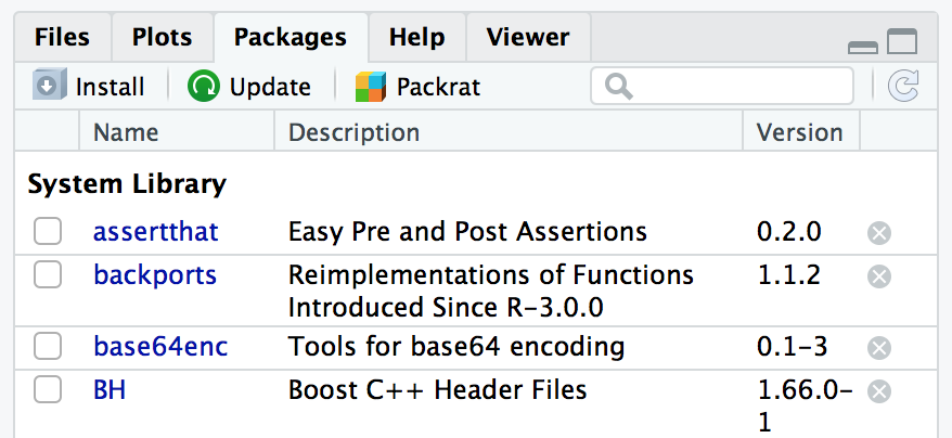
Installing a package locally is the first step toward using it. If you are installing packages outside of R Studio, the installer may prompt you for a mirror site from which it can download the package files. It will then display a list of CRAN mirror sites. Select one close to you.
The official CRAN server is a relatively modest machine generously hosted by the Department of Statistics and Mathematics at WU Wien, Vienna, Austria. If every R user downloaded from the official server, it would buckle under the load, so there are numerous mirror sites around the globe. In R Studio the default CRAN server is set to be the R Studio CRAN mirror. This is an excellent choice if you are in the USA. The R Studio CRAN mirror is accessable to all R users, not just those running the R Studio IDE.
If the new package depends upon other packages that are not already installed locally, then the R installer will automatically download and install those required packages. This is a huge benefit that frees you from the tedious task of identifying and resolving those dependencies.
There is a special consideration when installing on Linux or Unix. You can install the package either in the system-wide library or in your personal library. Packages in the system-wide library are available to everyone; packages in your personal library are (normally) used only by you. So a popular, well-tested package would likely go in the system-wide library whereas an obscure or untested package would go into your personal library.
By default, install.packages assumes you are performing a system-wide
install. If you do not have sufficient user permissions to install in
the system wide library location, R will ask if you would like to
install the package in a user library. The default that R suggests is
typically a good choice. However, if you would like to control the path
for your library location, you can use the lib= argument of the
install.packages function:
install.packages("packagename",lib="~/lib/R")
See “Finding Relevant Functions and Packages” for ways to find relevant packages and “Accessing the Functions in a Package” for using a package after installing it.
You’ve found an interesting package which you’d like to try. However, the author has not yet published the package on CRAN, but has published it on Github. You’d like to install the package directly from Github.
Ensure you have the devtools package installed and loaded:
Then use install_github and the name of the Github repository to
install directly from Github. For example, to install Thomas Lin
Pederson’s tidygraph package, you could execute the following:
install_github("thomasp85/tidygraph")
The devtools package is a package that contains helper functions for
installing R packages from remote (non-ss) repositories, like Github. If
a package has been built as an R package and then hosted on Github you
can install the package using the install_github function by passing
the Github username and repository name as a string parameter. You can
determine the Github username and repo name from the github URL, or from
the top of the Github page like in the example shown in ???.
. image::images_v2/github.shot.png[]
You are downloading packages. You want to set or change your default CRAN mirror.
In R Studio, you can change your default CRAN mirror from the R Studio Preferences menu shown in ???:
. image::images_v2/rstudio.package.pref.png[]
If you are running R without R Studio you can change your CRAN mirror
using the following solution. This solution assumes you have an
.Rprofile, as described in “Customizing R Startup”:
Call the choosessmirror function:
choosessmirror()
R will present a list of CRAN mirrors.
Select a CRAN mirror from the list and press OK.
To get the URL of the mirror, look at the first element of the
repos option:
options("repos")[[1]][1]
Add this line to your .Rprofile file. If you want the R Studio
CRAN mirror, you would do the following:
options(repos=c(CRAN="http://cran.rstudio.com"))
where URL is the URL of the mirror.
When you install packages, you probably use the same CRAN mirror each time (namely, the mirror closest to you or the R Studio mirror). You may want to change that mirror to use a different mirror that’s closer to you or controlled by your employer. Use this solution to change your repo so that every time you start R or R Studio you will be using your desired repo.
The repos option is the name of your default mirror. The
choosessmirror function has the important side effect of setting the
repos option according to your selection. The problem is that R
forgets the setting when it exits, leaving no permanent default. By
setting repos in your .Rprofile, you restore the setting every time
R starts.
See “Customizing R Startup” for
more about the .Rprofile file and the options function.
You captured a series of R commands in a text file. Now you want to execute them.
The source function instructs R to read the text file and execute its
contents:
source("myScript.R")
When you have a long or frequently used piece of R code, capture it
inside a text file. That lets you easily rerun the code without having
to retype it. Use the source function to read and execute the code,
just as if you had typed it into the R console.
Suppose the file hello.R contains this one, familiar greeting:
("Hello, World!")
Then sourcing the file will execute the file contents:
source("hello.R")#> [1] "Hello, World!"
Setting echo=TRUE will echo the script lines before they are executed,
with the R prompt shown before each line:
source("hello.R",echo=TRUE)#>#> > print("Hello, World!")#> [1] "Hello, World!"
See “Typing Less and Accomplishing More” for running blocks of R code inside the GUI.
You are writing a command script, such as a shell script in Unix or OS X or a BAT script in Windows. Inside your script, you want to execute an R script.
Run the R program with the CMD BATCH subcommand, giving the script
name and the output file name:
R CMD BATCH scriptfile outputfile
If you want the output sent to stdout or if you need to pass
command-line arguments to the script, consider the Rscript command
instead:
Rscript scriptfile arg1 arg2 arg3
R is normally an interactive program, one that prompts the user for input and then displays the results. Sometimes you want to run R in batch mode, reading commands from a script. This is especially useful inside shell scripts, such as scripts that include a statistical analysis.
The CMD BATCH subcommand puts R into batch mode, reading from
scriptfile and writing to outputfile. It does not interact with a user.
You will likely use command-line options to adjust R’s batch behavior to
your circumstances. For example, using --quiet silences the startup
messages that would otherwise clutter the output:
R CMD BATCH --quiet myScript.R results.out
Other useful options in batch mode include the following:
--slaveLike --quiet, but it makes R even more silent by inhibiting echo of
the input.
--no-restoreAt startup, do not restore the R workspace. This is important if your script expects R to begin with an empty workspace.
--no-saveAt exit, do not save the R workspace. Otherwise, R will save its
workspace and overwrite the .RData file in the working directory.
--no-init-fileDo not read either the .Rprofile or ~/.Rprofile files.
The CMD BATCH subcommand normally calls proc.time when your script
completes, showing the execution time. If this annoys you then end your
script by calling the q function with runLast=FALSE, which will
prevent the call to proc.time.
The CMD BATCH subcommand has two limitations: the output always goes
to a file, and you cannot easily pass command-line arguments to your
script. If either limitation is a problem, consider using the Rscript
program that comes with R. The first command-line argument is the script
name, and the remaining arguments are given to the script:
Rscript myScript.R arg1 arg2 arg3
Inside the script, the command-line arguments can be accessed by calling
commandArgs, which returns the arguments as a vector of strings:
argv<-commandArgs(TRUE)
The Rscript program takes the same command-line options as
CMD BATCH, which were just described.
Output is written to stdout, which R inherits from the calling shell script, of course. You can redirect the output to a file by using the normal redirection:
Rscript --slave myScript.R arg1 arg2 arg3 >results.out
Here is a small R script, arith.R, that takes two command-line
arguments and performs four arithmetic operations on them:
argv<-commandArgs(TRUE)x<-as.numeric(argv[1])y<-as.numeric(argv[2])cat("x =",x,"\n")cat("y =",y,"\n")cat("x + y = ",x+y,"\n")cat("x - y = ",x-y,"\n")cat("x * y = ",x*y,"\n")cat("x / y = ",x/y,"\n")
The script is invoked like this:
Rscript arith.R 2 3.1415
which produces the following output:
x=2y=3.1415x+y=5.1415x-y=-1.1415x*y=6.283x/y=0.6366385
On Linux, Unix, or Mac, you can make the script fully self-contained by
placing a #! line at the head with the path to the Rscript program.
Suppose that Rscript is installed in /usr/bin/Rscript on your
system. Then adding this line to arith.R makes it a self-contained
script:
#!/usr/bin/Rscript --slaveargv <- commandArgs(TRUE)x <- as.numeric(argv[1]). .(etc.).
At the shell prompt, we mark the script as executable:
chmod +x arith.R
Now we can invoke the script directly without the Rscript prefix:
arith.R 2 3.1415
See “Running a Script” for running a script from within R.
You need to know the R home directory, which is where the configuration and installation files are kept.
R creates an environment variable called R_HOME that you can access by
using the Sys.getenv function:
Sys.getenv("R_HOME")#> [1] "/Library/Frameworks/R.framework/Resources"
Most users will never need to know the R home directory. But system administrators or sophisticated users must know in order to check or change the R installation files.
When R starts, it defines an environment variable (not an R variable)
called R_HOME, which is the path to the R home directory. The
Sys.getenv function can retrieve its value. Here are examples by
platform. The exact value reported will almost certainly be different on
your own computer:
On Windows
> Sys.getenv("R_HOME") [1] "C:/PROGRA~1/R/R-34~1.4"
On OS X
> Sys.getenv("R_HOME")
[1] "/Library/Frameworks/R.framework/Resources"
On Linux or Unix
> Sys.getenv("R_HOME")
[1] "/usr/lib/R"
The Windows result looks funky because R reports the old, DOS-style
compressed path name. The full, user-friendly path would be
C:\Program Files\R\R-3.4.4 in this case.
On Unix and OS X, you can also run the R program from the shell and use
the RHOME subcommand to display the home directory:
R RHOME
# /usr/lib/R
Note that the R home directory on Unix and OS X contains the
installation files but not necessarily the R executable file. The
executable could be in /usr/bin while the R home directory is, for
example, /usr/lib/R.
You want to customize your R sessions by, for instance, changing configuration options or preloading packages.
Create a script called .Rprofile that customizes your R session. R
will execute the .Rprofile script when it starts. The placement of
.Rprofile depends upon your platform:
Save the file in your home directory (~/.Rprofile).
Save the file in your Documents directory.
R executes profile scripts when it starts, freeing you from repeatedly loading often-used packages or tweaking the R configuration options.
You can create a profile script called .Rprofile and place it in your
home directory (OS X, Linux, Unix) or your Documents directory
(Windows). The script can call functions to customize your sessions,
such as this simple script that sets two environment variables and sets
the console prompt to R>:
Sys.setenv(DB_USERID="my_id")Sys.setenv(DB_PASSWORD="My_Password!")options(prompt="R> ")
The profile script executes in a bare-bones environment, so there are limits on what it can do. Trying to open a graphics window will fail, for example, because the graphics package is not yet loaded. Also, you should not attempt long-running computations.
You can customize a particular project by putting an .Rprofile file in
the directory that contains the project files. When R starts in that
directory, it reads the local .Rprofile file; this allows you to do
project-specific customizations (e.g., setting your console prompt to a
specific project name). However, if R finds a local profile then it does
not read the global profile. That can be annoying, but it’s easily
fixed: simply source the global profile from the local profile. On
Unix, for instance, this local profile would execute the global profile
first and then execute its local material:
source("~/.Rprofile")## ... remainder of local .Rprofile...#
Some customizations are handled via calls to the options function,
which sets the R configuration options. There are many such options, and
the R help page for options lists them all:
help(options)
Here are some examples:
browser="path"Path of default HTML browser
digits=nSuggested number of digits to print when printing numeric values
editor="path"Default text editor
prompt="string"Input prompt
repos="url"URL for default repository for packages
warn=nControls display of warning messages
Many of us use certain packages over and over in all of our script. For
example, we use the tidyverse packages in almost all our scripts. It
is tempting to load these packages in your .Rprofile so that they are
always available without typing anything. As a matter of fact, this
advice was given in the first edition of this book. However, the
downside of loading packages in your .Rprofile is reproducibility. If
someone else (or you, on another machine) tries to run your script, they
may not realize that you had loaded packages in your .Rprofile. Your
script might not work for them, depending on which packages they load.
So while it might be convenient to load packages in .Rprofile you will
play better with collaborators (and your future self) if you explicitly
call library(packagename) in your R scripts.
Another issue with reproducability and the .Rprofile is when users
change calculation default behaviors of R inside their .Rprofile. An
example of this would be setting options(stringsAsFactors = FALSE).
This is appealing as many users would prefer this default. However, if
someone runs the script without this option being set, they will get
different results or not be able to run the script at all. This can lead
to considerable frustration.
As a guideline, you should primarly put things in the .Rprofile that:
Change the look and feel of R (e.g. digits)
Are specific to your local environment (e.g. browser)
Specifically need to be outside of your scripts (i.e. database passwords)
Do not change the results of your analysis.
Here is a simplified overview of what happens when R starts (type
help(Startup) to see the full details):
R executes the Rprofile.site script. This is the site-level
script that enables system administrators to override default options
with localizations. The script’s full path is
R_HOME\\/etc/Rprofile.site. (R_HOME is the R home directory; see
“Locating the R Home Directory”.)
The R distribution does not include an Rprofile.site file. Rather, the
system administrator creates one if it is needed.
R executes the .Rprofile script in the working directory; or, if
that file does not exist, executes the .Rprofile script in your home
directory. This is the user’s opportunity to customize R for his or her
purposes. The .Rprofile script in the home directory is used for
global customizations. The .Rprofile script in a lower-level directory
can perform specific customizations when R is started there; for
instance, customizing R when started in a project-specific directory.
R loads the workspace saved in .RData, if that file exists in the
working directory. R saves your workspace in the file called .RData
when it exits. It reloads your workspace from that file, restoring
access to your local variables and functions. This can be disabled in R
Studio through Tools → Global Options. We recommend you disable this
and always explicitly save and load your work.
R executes the`.First`function, if you defined one. The .First
function is a useful place for users or projects to define startup
initialization code. You can define it in your .Rprofile or in your
workspace.
R executes the`.First.sys`function. This step loads the default packages. The function is internal to R and not normally changed by either users or administrators.
Observe that R does not load the default packages until the final step,
when it executes the .First.sys function. Before that, only the base
package has been loaded. This is a key fact because it means the
previous steps cannot assume that packages other than the base are
available. It also explains why trying to open a graphical window in
your .Rprofile script fails: the graphics packages aren’t loaded yet.
See “Accessing the Functions in a Package” for more about loading packages. See the R help
page for Startup (help(Startup)) and the R help page for options
(help(options)).
You want to run R and R Studio in a cloud environment.
The most straightforward way to use R in the cloud is to use the RStudio.cloud web service. To use the service, point your web browser to http://rstudio.cloud and set up an account, or log in with your Google or Github credentials.
After you log in, click New Project to begin a new R Studio session in
a new workspace. You’ll be greeted by the familiar R Studio interface
shown in Figure 3-4.

It’s worth keeping in mind that as of the writing of this book the RStudio.cloud service is in alpha testing and may not be 100% stable. Your work will persist after you log off. However, as with any system, it is a good idea to ensure you have backups of all the work you do. A common work pattern is to connect your project in RStudio.cloud to a GitHub.com repository and push your changes frequently from Rstudio.cloud to GitHub. This workflow has been used significantly in the writing of this book.
Use of git and GitHub are beyond the scope of this book, but if you
are interested in learning more, we highly recommend Jenny Bryan’s web
book Happy Git and GitHub for the useR http://happygitwithr.com/
In its current Alpha state, each RStudio.cloud session is limited to 1 GB of RAM and 3 GB of drive space. So it’s a great platform for learning and teaching but might not (yet) be the platform on which you want to build a commercial data science laboratory. R Studio has expressed intent to offer greater processing power and storage as part of a paid tier of service as the platform matures.
If you are needing more computing power than offered by RStudio.cloud and you are willing to pay for the services, both Amazon AWS and Google Cloud Platform offer cloud based R Studio offerings. Other cloud platforms that support Docker, such as Digital Ocean, are also reasonable options for cloud hosted R Studio.
Running R Studio Pro on Google Cloud Platform: https://console.cloud.google.com/marketplace/details/rstudio-launcher-public/rstudio-server-pro-for-gcp
Running R Studio Pro on Amazon Web Services: https://aws.amazon.com/marketplace/pp/B06W2G9PRY
How To Set Up RStudio On Digital Ocean: https://www.digitalocean.com/community/tutorials/how-to-set-up-rstudio-on-an-ubuntu-cloud-server
***todo: add base R options at end of tidy recipes?
All statistical work begins with data, and most data is stuck inside files and databases. Dealing with input is probably the first step of implementing any significant statistical project.
All statistical work ends with reporting numbers back to a client, even if you are the client. Formatting and producing output is probably the climax of your project.
Casual R users can solve their input problems by using basic functions
such as read.csv to read CSV files and read.table to read more
complicated, tabular data. They can use print, cat, and format to
produce simple reports.
Users with heavy-duty input/output (I/O) needs are strongly encouraged to read the R Data Import/Export guide, available on CRAN at http://cran.r-project.org/doc/manuals/R-data.pdf. This manual includes important information on reading data from sources such as spreadsheets, binary files, other statistical systems, and relational databases.
You have a small amount of data, too small to justify the overhead of creating an input file. You just want to enter the data directly into your workspace.
For very small datasets, enter the data as literals using the c()
constructor for vectors:
scores<-c(61,66,90,88,100)
When working on a simple problem, you may not want the hassle of
creating and then reading a data file outside of R. You may just want to
enter the data into R. The easiest way is by using the c() constructor
for vectors, as shown in the Solution.
This approach works for data frames, too, by entering each variable (column) as a vector:
points<-data.frame(label=c("Low","Mid","High"),lbound=c(0,0.67,1.64),ubound=c(0.67,1.64,2.33))
See Recipe X-X for more about using the built-in data editor, as suggested in the Solution.
For cutting and pasting data from another application into R, be sure
and look at datapasta, a package that provides R Studio addins that
make pasting data into your scripts easier:
https://github.com/MilesMcBain/datapasta
Your output contains too many digits or too few digits. You want to print fewer or more.
For print, the digits parameter can control the number of printed
digits.
For cat, use the format function (which also has a digits
parameter) to alter the formatting of numbers.
R normally formats floating-point output to have seven digits:
pi#> [1] 3.14100*pi#> [1] 314
This works well most of the time but can become annoying when you have lots of numbers to print in a small space. It gets downright misleading when there are only a few significant digits in your numbers and R still prints seven.
The print function lets you vary the number of printed digits using
the digits parameter:
(pi,digits=4)#> [1] 3.142(100*pi,digits=4)#> [1] 314.2
The cat function does not give you direct control over formatting.
Instead, use the format function to format your numbers before calling
cat:
cat(pi,"\n")#> 3.14cat(format(pi,digits=4),"\n")#> 3.142
This is R, so both print and format will format entire vectors at
once:
pnorm(-3:3)#> [1] 0.00135 0.02275 0.15866 0.50000 0.84134 0.97725 0.99865(pnorm(-3:3),digits=3)#> [1] 0.00135 0.02275 0.15866 0.50000 0.84134 0.97725 0.99865
Notice that print formats the vector elements consistently: finding
the number of digits necessary to format the smallest number and then
formatting all numbers to have the same width (though not necessarily
the same number of digits). This is extremely useful for formating an
entire table:
q<-seq(from=0,to=3,by=0.5)tbl<-data.frame(Quant=q,Lower=pnorm(-q),Upper=pnorm(q))tbl# Unformatted print#> Quant Lower Upper#> 1 0.0 0.50000 0.500#> 2 0.5 0.30854 0.691#> 3 1.0 0.15866 0.841#> 4 1.5 0.06681 0.933#> 5 2.0 0.02275 0.977#> 6 2.5 0.00621 0.994#> 7 3.0 0.00135 0.999(tbl,digits=2)# Formatted print: fewer digits#> Quant Lower Upper#> 1 0.0 0.5000 0.50#> 2 0.5 0.3085 0.69#> 3 1.0 0.1587 0.84#> 4 1.5 0.0668 0.93#> 5 2.0 0.0228 0.98#> 6 2.5 0.0062 0.99#> 7 3.0 0.0013 1.00
You can also alter the format of all output by using the options
function to change the default for digits:
pi#> [1] 3.14options(digits=15)pi#> [1] 3.14159265358979
But this is a poor choice in our experience, since it also alters the output from R’s built-in functions, and that alteration may likely be unpleasant.
Other functions for formatting numbers include sprintf and formatC;
see their help pages for details.
You want to redirect the output from R into a file instead of your console.
You can redirect the output of the cat function by using its file
argument:
cat("The answer is",answer,"\n",file="filename.txt")
Use the sink function to redirect all output from both print and
cat. Call sink with a filename argument to begin redirecting console
output to that file. When you are done, use sink with no argument to
close the file and resume output to the console:
sink("filename")# Begin writing output to file# ... other session work ...sink()# Resume writing output to console
The print and cat functions normally write their output to your
console. The cat function writes to a file if you supply a file
argument, which can be either a filename or a connection. The print
function cannot redirect its output, but the sink function can force all
output to a file. A common use for sink is to capture the output of an R
script:
sink("script_output.txt")# Redirect output to filesource("script.R")# Run the script, capturing its outputsink()# Resume writing output to console
If you are repeatedly cat`ing items to one file, be sure to set
`append=TRUE. Otherwise, each call to cat will simply overwrite the
file’s contents:
cat(data,file="analysisReport.out")cat(results,file="analysisRepart.out",append=TRUE)cat(conclusion,file="analysisReport.out",append=TRUE)
Hard-coding file names like this is a tedious and error-prone process. Did you notice that the filename is misspelled in the second line? Instead of hard-coding the filename repeatedly, I suggest opening a connection to the file and writing your output to the connection:
con<-file("analysisReport.out","w")cat(data,file=con)cat(results,file=con)cat(conclusion,file=con)close(con)
(You don’t need append=TRUE when writing to a connection because
append is the default with connections.) This technique is especially
valuable inside R scripts because it makes your code more reliable and
more maintainable.
You want an R vector that is a listing of the files in your working directory.
The list.files function shows the contents of your working directory:
list.files()#> [1] "_book" "_bookdown_files"#> [3] "_bookdown_files.old" "_bookdown.yml"#> [5] "_common.R" "_main.rds"#> [7] "_output.yaml" "01_GettingStarted_cache"#> [9] "01_GettingStarted.md" "01_GettingStarted.Rmd"etc...
This function is terribly handy to grab the names of all files in a subdirectory. You can use it to refresh your memory of your file names or, more likely, as input into another process, like importing data files.
You can pass list.files a path and a pattern to shows files in a
specific path and matching a specific regular expression pattern.
list.files(path='data/')# show files in a directory#> [1] "ac.rdata" "adf.rdata"#> [3] "anova.rdata" "anova2.rdata"#> [5] "bad.rdata" "batches.rdata"#> [7] "bnd_cmty.Rdata" "compositePerf-2010.csv"#> [9] "conf.rdata" "daily.prod.rdata"#> [11] "data1.csv" "data2.csv"#> [13] "datafile_missing.tsv" "datafile.csv"#> [15] "datafile.fwf" "datafile.qsv"#> [17] "datafile.ssv" "datafile.tsv"#> [19] "df_decay.rdata" "df_squared.rdata"#> [21] "diffs.rdata" "example1_headless.csv"#> [23] "example1.csv" "excel_table_data.xlsx"#> [25] "get_USDA_NASS_data.R" "ibm.rdata"#> [27] "iris_excel.xlsx" "lab_df.rdata"#> [29] "movies.sas7bdat" "nacho_data.csv"#> [31] "NearestPoint.R" "not_a_csv.txt"#> [33] "opt.rdata" "outcome.rdata"#> [35] "pca.rdata" "pred.rdata"#> [37] "pred2.rdata" "sat.rdata"#> [39] "singles.txt" "state_corn_yield.rds"#> [41] "student_data.rdata" "suburbs.txt"#> [43] "tab1.csv" "tls.rdata"#> [45] "triples.txt" "ts_acf.rdata"#> [47] "workers.rdata" "world_series.csv"#> [49] "xy.rdata" "yield.Rdata"#> [51] "z.RData"list.files(path='data/',pattern='\\.csv')#> [1] "compositePerf-2010.csv" "data1.csv"#> [3] "data2.csv" "datafile.csv"#> [5] "example1_headless.csv" "example1.csv"#> [7] "nacho_data.csv" "tab1.csv"#> [9] "world_series.csv"
To see all the files in your subdirectories, too, use
list.files(recursive=T)
A possible “gotcha” of list.files is that it ignores hidden
files—typically, any file whose name begins with a period. If you don’t
see the file you expected to see, try setting all.files=TRUE:
list.files(path='data/',all.files=TRUE)#> [1] "." ".."#> [3] ".DS_Store" ".hidden_file.txt"#> [5] "ac.rdata" "adf.rdata"#> [7] "anova.rdata" "anova2.rdata"#> [9] "bad.rdata" "batches.rdata"#> [11] "bnd_cmty.Rdata" "compositePerf-2010.csv"#> [13] "conf.rdata" "daily.prod.rdata"#> [15] "data1.csv" "data2.csv"#> [17] "datafile_missing.tsv" "datafile.csv"#> [19] "datafile.fwf" "datafile.qsv"#> [21] "datafile.ssv" "datafile.tsv"#> [23] "df_decay.rdata" "df_squared.rdata"#> [25] "diffs.rdata" "example1_headless.csv"#> [27] "example1.csv" "excel_table_data.xlsx"#> [29] "get_USDA_NASS_data.R" "ibm.rdata"#> [31] "iris_excel.xlsx" "lab_df.rdata"#> [33] "movies.sas7bdat" "nacho_data.csv"#> [35] "NearestPoint.R" "not_a_csv.txt"#> [37] "opt.rdata" "outcome.rdata"#> [39] "pca.rdata" "pred.rdata"#> [41] "pred2.rdata" "sat.rdata"#> [43] "singles.txt" "state_corn_yield.rds"#> [45] "student_data.rdata" "suburbs.txt"#> [47] "tab1.csv" "tls.rdata"#> [49] "triples.txt" "ts_acf.rdata"#> [51] "workers.rdata" "world_series.csv"#> [53] "xy.rdata" "yield.Rdata"#> [55] "z.RData"
If you just want to see which files are in a directory and not use the
file names in a procedure, the easiest way is to open the Files pane
in the lower right corner of RStudio. But keep in mind that the RStudio
Files pane hides files that start with a . as you can see in ???:
. image::images_v2/rstudio.files2.png[]
R has other handy functions for working with files; see help(files).
You are running R on Windows, and you are using file names such as
C:\data\sample.txt. R says it cannot open the file, but you know the
file does exist.
The backslashes in the file path are causing trouble. You can solve this problem in one of two ways:
Change the backslashes to forward slashes: "C:/data/sample.txt".
Double the backslashes: "C:\\data\\sample.txt".
When you open a file in R, you give the file name as a character string.
Problems arise when the name contains backslashes (\) because
backslashes have a special meaning inside strings. You’ll probably get
something like this:
samp<-read_csv("C:\Data\sample-data.csv")#> Error: '\D' is an unrecognized escape in character string starting ""C:\D"
R escapes every character that follows a backslash and then removes the
backslashes. That leaves a meaningless file path, such as
C:Datasample-data.csv in this example.
The simple solution is to use forward slashes instead of backslashes. R leaves the forward slashes alone, and Windows treats them just like backslashes. Problem solved:
samp<-read_csv("C:/Data/sample-data.csv")
An alternative solution is to double the backslashes, since R replaces two consecutive backslashes with a single backslash:
samp<-read_csv("C:\\Data\\sample-data.csv")
You are reading data from a file of fixed-width records: records whose data items occur at fixed boundaries.
Use the read_fwf from the readr package (which is part of the
tidyverse). The main arguments are the file name and the description of
the fields:
library(tidyverse)records<-read_fwf("./data/datafile.fwf",fwf_cols(last=10,first=10,birth=5,death=5))#> Parsed with column specification:#> cols(#> last = col_character(),#> first = col_character(),#> birth = col_double(),#> death = col_double()#> )records#> # A tibble: 5 x 4#> last first birth death#> <chr> <chr> <dbl> <dbl>#> 1 Fisher R.A. 1890 1962#> 2 Pearson Karl 1857 1936#> 3 Cox Gertrude 1900 1978#> 4 Yates Frank 1902 1994#> 5 Smith Kirstine 1878 1939
For reading in data into R, we highly recommend the readr package.
There are base R functions for reading in text files, but readr
improves on these base functions with faster performance, better
defaults, and more flexibility.
Suppose we want to read an entire file of fixed-width records, such as
fixed-width.txt, shown here:
Fisher    R.A.      1890 1962
Pearson   Karl      1857 1936
Cox       Gertrude  1900 1978
Yates     Frank     1902 1994
Smith     Kirstine  1878 1939
We need to know the column widths. In this case the columns are:
Last name, 10 characters
First name, 10 characters
Year of birth, 5 characters
Year of death, 5 characters
There are 5 different ways to define the columns using read_fwf. Pick
the one that’s easiest to use (or remember) in your situation:
read_fwf can try to guess your column widths if there is empty
space between the columns with the `fwf_empty`option:
file<-"./data/datafile.fwf"t1<-read_fwf(file,fwf_empty(file,col_names=c("last","first","birth","death")))#> Parsed with column specification:#> cols(#> last = col_character(),#> first = col_character(),#> birth = col_double(),#> death = col_double()#> )
You can define each column by a vector of widths followed by a
vector of names with with fwf_widths:
t2<-read_fwf(file,fwf_widths(c(10,10,5,4),c("last","first","birth","death")))#> Parsed with column specification:#> cols(#> last = col_character(),#> first = col_character(),#> birth = col_double(),#> death = col_double()#> )
The columns can be defined with fwf_cols which takes a series of
column names followed by the column widths:
t3<-read_fwf("./data/datafile.fwf",fwf_cols(last=10,first=10,birth=5,death=5))#> Parsed with column specification:#> cols(#> last = col_character(),#> first = col_character(),#> birth = col_double(),#> death = col_double()#> )
Each column can be defined by a begining position and ending
poaition with fwf_cols:
t4<-read_fwf(file,fwf_cols(last=c(1,10),first=c(11,20),birth=c(21,25),death=c(26,30)))#> Parsed with column specification:#> cols(#> last = col_character(),#> first = col_character(),#> birth = col_double(),#> death = col_double()#> )
You can also define the columns with a vector of starting positions,
a vector of ending positions, and a vector of column names with
fwf_positions:
t5<-read_fwf(file,fwf_positions(c(1,11,21,26),c(10,20,25,30),c("first","last","birth","death")))#> Parsed with column specification:#> cols(#> first = col_character(),#> last = col_character(),#> birth = col_double(),#> death = col_double()#> )
The read_fwf returns a tibble which is a tidyverse object very
similiar to a data frame. As is common with tidyverse packages,
read_fwf has a good selection of default assumptions that make it less
tricky to use than some base R functions for importing data. For
example, `read_fwf_ will, by default, import character fields as
characters, not factors, which prevents much pain and consternation for
users.
See “Reading Tabular Data Files” for more discussion of reading text files.
You want to read a text file that contains a table of white-space delimited data.
Use the read_table2 function from the readr package, which returns a
tibble:
library(tidyverse)tab1<-read_table2("./data/datafile.tsv")#> Parsed with column specification:#> cols(#> last = col_character(),#> first = col_character(),#> birth = col_double(),#> death = col_double()#> )tab1#> # A tibble: 5 x 4#> last first birth death#> <chr> <chr> <dbl> <dbl>#> 1 Fisher R.A. 1890 1962#> 2 Pearson Karl 1857 1936#> 3 Cox Gertrude 1900 1978#> 4 Yates Frank 1902 1994#> 5 Smith Kirstine 1878 1939
Tabular data files are quite common. They are text files with a simple format:
Each line contains one record.
Within each record, fields (items) are separated by a white space delimiter, such as a space or tab.
Each record contains the same number of fields.
This format is more free-form than the fixed-width format because fields needn’t be aligned by position. Here is the data file from “Reading Fixed-Width Records” in tabular format, using a tab character between fields:
last    first   birth   death
Fisher  R.A.    1890    1962
Pearson Karl    1857    1936
Cox Gertrude    1900    1978
Yates   Frank   1902    1994
Smith   Kirstine    1878    1939
The read_table2 function is designed to make some good guesses about
your data. It assumes your data has column names in the first row,
guesses your delimiter, and it imputes your column types based on the
first 1000 records in your data set. Below is an example with space
delimited data.
t<-read_table2("./data/datafile.ssv")#> Parsed with column specification:#> cols(#> `#The` = col_character(),#> following = col_character(),#> is = col_character(),#> a = col_character(),#> list = col_character(),#> of = col_character(),#> statisticians = col_character()#> )#> Warning: 6 parsing failures.#> row col expected actual file#> 1 -- 7 columns 4 columns './data/datafile.ssv'#> 2 -- 7 columns 4 columns './data/datafile.ssv'#> 3 -- 7 columns 4 columns './data/datafile.ssv'#> 4 -- 7 columns 4 columns './data/datafile.ssv'#> 5 -- 7 columns 4 columns './data/datafile.ssv'#> ... ... ......... ......... .....................#> See problems(...) for more details.(t)#> # A tibble: 6 x 7#> `#The` following is a list of statisticians#> <chr> <chr> <chr> <chr> <chr> <chr> <chr>#> 1 last first birth death <NA> <NA> <NA>#> 2 Fisher R.A. 1890 1962 <NA> <NA> <NA>#> 3 Pearson Karl 1857 1936 <NA> <NA> <NA>#> 4 Cox Gertrude 1900 1978 <NA> <NA> <NA>#> 5 Yates Frank 1902 1994 <NA> <NA> <NA>#> 6 Smith Kirstine 1878 1939 <NA> <NA> <NA>
read_table2 often guess corectly. But as with other readr import
functions, you can overwrite the defaults with explicit parameters.
t<-read_table2("./data/datafile.tsv",col_types=c(col_character(),col_character(),col_integer(),col_integer()))
If any field contains the string “NA”, then read_table2 assumes that
the value is missing and converts it to NA. Your data file might employ
a different string to signal missing values, in which case use the na
parameter. The SAS convention, for example, is that missing values are
signaled by a single period (.). We can read such text files using the
na="." option. If we have a file named datafile_missing.tsv that has
a missing value indicated with a . in the last row:
last    first   birth   death
Fisher  R.A.    1890    1962
Pearson Karl    1857    1936
Cox Gertrude    1900    1978
Yates   Frank   1902    1994
Smith   Kirstine    1878    1939
Cox David 1924 .
we can import it like so
t<-read_table2("./data/datafile_missing.tsv",na=".")#> Parsed with column specification:#> cols(#> last = col_character(),#> first = col_character(),#> birth = col_double(),#> death = col_double()#> )t#> # A tibble: 6 x 4#> last first birth death#> <chr> <chr> <dbl> <dbl>#> 1 Fisher R.A. 1890 1962#> 2 Pearson Karl 1857 1936#> 3 Cox Gertrude 1900 1978#> 4 Yates Frank 1902 1994#> 5 Smith Kirstine 1878 1939#> 6 Cox David 1924 NA
We’re huge fans of self-describing data: data files which describe their
own contents. (A computer scientist would say the file contains its own
metadata.) The read_table2 function make the default assumption that
the first line of your file contains a header line with column names. If
your file does not have column names, you can turn this off with the
parameter col_names = FALSE.
An additional type of metadata supported by read_table2 is comment
lines. Using the comment parameter you can tell read_table2 which
character distinguishes comment lines. The following file has a comment
line at the top that starts with #.
# The following is a list of statisticians
last first birth death
Fisher R.A. 1890 1962
Pearson Karl 1857 1936
Cox Gertrude 1900 1978
Yates Frank 1902 1994
Smith Kirstine 1878 1939
so we can import this file as follows:
t<-read_table2("./data/datafile.ssv",comment='#')#> Parsed with column specification:#> cols(#> last = col_character(),#> first = col_character(),#> birth = col_double(),#> death = col_double()#> )t#> # A tibble: 5 x 4#> last first birth death#> <chr> <chr> <dbl> <dbl>#> 1 Fisher R.A. 1890 1962#> 2 Pearson Karl 1857 1936#> 3 Cox Gertrude 1900 1978#> 4 Yates Frank 1902 1994#> 5 Smith Kirstine 1878 1939
read_table2 has many parameters for controlling how it reads and
interprets the input file. See the help page (?read_table2) or the
readr vignette (vignette("readr")) for more details. If you’re
curious about the difference between read_table and read_table2,
it’s in the help file… but the short answer is that read_table is
slightly less forgiving in file structure and line length.
If your data items are separated by commas, see “Reading from CSV Files” for reading a CSV file.
You want to read data from a comma-separated values (CSV) file.
The read_csv function from the readr pacakge is a fast (and,
according to the documentation, fun) way to read CSV files. If your CSV
file has a header line, use this:
library(tidyverse)tbl<-read_csv("./data/datafile.csv")#> Parsed with column specification:#> cols(#> last = col_character(),#> first = col_character(),#> birth = col_double(),#> death = col_double()#> )
If your CSV file does not contain a header line, set the col_names
option to FALSE:
tbl<-read_csv("./data/datafile.csv",col_names=FALSE)#> Parsed with column specification:#> cols(#> X1 = col_character(),#> X2 = col_character(),#> X3 = col_character(),#> X4 = col_character()#> )
The CSV file format is popular because many programs can import and export data in that format. This includes R, Excel, other spreadsheet programs, many database managers, and most statistical packages. It is a flat file of tabular data, where each line in the file is a row of data, and each row contains data items separated by commas. Here is a very simple CSV file with three rows and three columns (the first line is a header line that contains the column names, also separated by commas):
label,lbound,ubound
low,0,0.674
mid,0.674,1.64
high,1.64,2.33
The read_csv file reads the data and creates a tibble, which is a
special type of data frame used in Tidy packages and a common
representation for tabular data. The function assumes that your file has
a header line unless told otherwise:
tbl<-read_csv("./data/example1.csv")#> Parsed with column specification:#> cols(#> label = col_character(),#> lbound = col_double(),#> ubound = col_double()#> )tbl#> # A tibble: 3 x 3#> label lbound ubound#> <chr> <dbl> <dbl>#> 1 low 0 0.674#> 2 mid 0.674 1.64#> 3 high 1.64 2.33
Observe that read_csv took the column names from the header line for
the tibble. If the file did not contain a header, then we would specify
col_names=FALSE and R would synthesize column names for us (X1,
X2, and X3 in this case):
tbl<-read_csv("./data/example1.csv",col_names=FALSE)#> Parsed with column specification:#> cols(#> X1 = col_character(),#> X2 = col_character(),#> X3 = col_character()#> )tbl#> # A tibble: 4 x 3#> X1 X2 X3#> <chr> <chr> <chr>#> 1 label lbound ubound#> 2 low 0 0.674#> 3 mid 0.674 1.64#> 4 high 1.64 2.33
Sometimes it’s convenient to put metadata in files. If this metadata
starts with a common character, such as a pound sign (#) we can use
the comment=FALSE parameter to ignore metadata lines.
The read_csv function has many useful bells and whistles. A few of
these options and their default values include:
na = c("", "NA"): Indicate what values represent missing or NA
values
comment = "": which lines to ignore as comments or metadata
trim_ws = TRUE: Whether to drop white space at the beginning and/or
end of fields
skip = 0: Number of rows to skip at the beginning of the file
guess_max = min(1000, n_max): Number of rows to consider when
imputing column types
See the R help page, help(read_csv), for more details on all the
availiable options.
If you have a data file that uses semicolons (;) for seperators and
commas for the decimal mark, as is common outside of North America, then
you should use the function read_csv2 which is built for that very
situation.
See “Writing to CSV Files”. See also the vignette for the readr: vignette(readr).
You want to save a matrix or data frame in a file using the comma-separated values format.
The write_csv function from the tidyverse readr package can write a
CSV file:
library(tidyverse)write_csv(tab1,path="./data/tab1.csv")
The write_csv function writes tabular data to an ASCII file in CSV
format. Each row of data creates one line in the file, with data items
separated by commas (,):
library(tidyverse)(tab1)#> # A tibble: 5 x 4#> last first birth death#> <chr> <chr> <dbl> <dbl>#> 1 Fisher R.A. 1890 1962#> 2 Pearson Karl 1857 1936#> 3 Cox Gertrude 1900 1978#> 4 Yates Frank 1902 1994#> 5 Smith Kirstine 1878 1939write_csv(tab1,"./data/tab1.csv")
This example creates a file called tab1.csv in the data directory
which is a subdirectory of the working directory. The file looks like
this:
last,first,birth,death
Fisher,R.A.,1890,1962
Pearson,Karl,1857,1936
Cox,Gertrude,1900,1978
Yates,Frank,1902,1994
Smith,Kirstine,1878,1939
write_csv has a number of parameters with typically very good
defaults. Should you want to adjust the output, here are a few
parameters you can change, along with their defaults:
col_names = TRUE
: Indicate whether or not the first row contains column names
col_types = NULL
: write_csv will look at the first 1000 rows (changable with
guess_max below) and make an informed guess as to what data types to
use for the columns. If you’d rather explicitly state the column types,
you can do that by passing a vector of column types to the parameter
col_types
na = c("", "NA")
: Indicate what values represent missing or NA values
comment = ""
: Which lines to ignore as comments or metadata
trim_ws = TRUE
: Whether to drop white space at the beginning and/or end of fields
skip = 0
: Number of rows to skip at the beginning of the file
guess_max = min(1000, n_max)
: Number of rows to consider when guessing column types
See “Getting and Setting the Working Directory” for more about the current working directory and
“Saving and Transporting Objects” for other ways to save data to files. For more info on reading
and writing text files, see the readr vignette: vignette(readr).
You want to read data directly from the Web into your R workspace.
Use the the read_csv or read_table2 functions from the readr
package, using a URL instead of a file name. The functions will read
directly from the remote server:
library(tidyverse)berkley<-read_csv('http://bit.ly/barkley18',comment='#')#> Parsed with column specification:#> cols(#> Name = col_character(),#> Location = col_character(),#> Time = col_time(format = "")#> )
You can also open a connection using the URL and then read from the connection, which may be preferable for complicated files.
The Web is a gold mine of data. You could download the data into a file
and then read the file into R, but it’s more convenient to read directly
from the Web. Give the URL to read_csv, read_table2, or other read
function in readr (depending upon the format of the data), and the
data will be downloaded and parsed for you. No fuss, no muss.
Aside from using a URL, this recipe is just like reading from a CSV file (“Reading from CSV Files”) or a complex file (“Reading Files with a Complex Structure”), so all the comments in those recipes apply here, too.
Remember that URLs work for FTP servers, not just HTTP servers. This means that R can also read data from FTP sites using URLs:
tbl<-read_table2("ftp://ftp.example.com/download/data.txt")
You want to read data in from an Excel file.
The openxlsx package makes reading Excel files easy.
library(openxlsx)df1<-read.xlsx(xlsxFile="data/iris_excel.xlsx",sheet='iris_data')head(df1,3)#> Sepal.Length Sepal.Width Petal.Length Petal.Width Species#> 1 5.1 3.5 1.4 0.2 setosa#> 2 4.9 3.0 1.4 0.2 setosa#> 3 4.7 3.2 1.3 0.2 setosa
The package openxlsx is a good choice for both reading and writing
Excel files with R. If we’re reading in an entire sheet then passing a
file name and a sheet name to the read.xlsx function is a simple
option. But openxlsx supports more complex workflows.
A common pattern is to read a named table out of an Excel file and into
an R data frame. This is trickier because the sheet we’re reading from
may have values outside of the named table and we want to only read in
the named table range. We can use the functions in openxlsx to get the
location of a table, then read that range of cells into a data frame.
First we load the workbook into R:
library(openxlsx)wb<-loadWorkbook("data/excel_table_data.xlsx")
Then we can use the getTables function to get a the names and ranges
of all the Excel Tables in the input_data sheet and select out the one
table we want. In this example the Excel Table we are after is named
example_data:
tables<-getTables(wb,'input_data')table_range_str<-names(tables[tables=='example_table'])table_range_refs<-strsplit(table_range_str,':')[[1]]# use a regex to extract out the row numberstable_range_row_num<-gsub("[^0-9.]","",table_range_refs)# extract out the column numberstable_range_col_num<-convertFromExcelRef(table_range_refs)
Now the vector col_vec contains the column numbers of our named table
while table_range_row_num contains the row numbers of our named table.
We can then use the read.xlsx function to pull in only the rows and
columns we are after.
df<-read.xlsx(xlsxFile="data/excel_table_data.xlsx",sheet='input_data',cols=table_range_col_num[1]:table_range_col_num[2],rows=table_range_row_num[1]:table_range_row_num[2])
Vingette for openxlsx by installing openxlsx and running:
vignette('Introduction', package='openxlsx')
The readxl package is party of the Tidyverse and provides fast, simple
reading of Excel files: https://readxl.tidyverse.org/
The writexl package is a fast and lightweight (no dependencies)
package for writing Excel files:
https://cran.r-project.org/web/packages/writexl/index.html
You want to write an R data frame to an Excel file.
The openxlsx package makes writing to Excel files realitivly easy.
While there are lots of options in openxlsx, a typical pattern is to
specify an Excel file name and a sheet name:
library(openxlsx)write.xlsx(x=iris,sheetName='iris_data',file="data/iris_excel.xlsx")
The openxlsx package has a huge number of options for controlling many
aspects of the Excel object model. We can use it to set cell colors,
define named ranges, and set cell outlines, for example. But it has a
few helper functions like write.xlsx which make simple tasks easier.
When businesses work with Excel it’s a good practice to keep all input
data in an Excel file in a named Excel Table which makes accessing the
data easier and less error prone. However if you use openxlsx to
overwrite an Excel Table in one of the sheets, you run the risk that the
new data may contain fewer rows than the Excel Table it replaces. That
could cause errors as you would end up with old data and new data in
contiguious rows. The solution is to first delete out an existing Excel
Table, then add new data back into the same location and assign the new
data to a named Excel Table. To do this we need to use the more advanced
Excel manipulation features of openxlsx.
First we use loadWorkbook to read the Excel workbook into R in its
entirety:
library(openxlsx)wb<-loadWorkbook("data/excel_table_data.xlsx")
Before we delete the table out we want to extract the table starting row and column.
tables<-getTables(wb,'input_data')table_range_str<-names(tables[tables=='example_table'])table_range_refs<-strsplit(table_range_str,':')[[1]]# use a regex to extract out the starting row numbertable_row_num<-gsub("[^0-9.]","",table_range_refs)[[1]]# extract out the starting column numbertable_col_num<-convertFromExcelRef(table_range_refs)[[1]]
Then we can use the removeTable function to remove the existing named
Excel Table:
## remove the existing Excel TableremoveTable(wb=wb,sheet='input_data',table='example_table')
Then we can use writeDataTable to write the iris data frame (which
comes with R) to write data back into our workbook object in R.
writeDataTable(wb=wb,sheet='input_data',x=iris,startCol=table_col_num,startRow=table_row_num,tableStyle="TableStyleLight9",tableName='example_table')
At this point we could save the workbook and our Table would be updated.
However it’s a good idea to save some meta data in the workbook to let
others know exactly when the data was refreshed. We can do this with the
writeData function then save the workbook to file and overwrite the
original file. We’ll put the text in cell B:5 then save the workbook
back to a file overwriting the original.
writeData(wb=wb,sheet='input_data',x=paste('example_table data refreshed on:',Sys.time()),startCol=2,startRow=5)## then save the workbooksaveWorkbook(wb=wb,file="data/excel_table_data.xlsx",overwrite=T)
The resulting Excel sheet looks is shown in Figure 4-1.
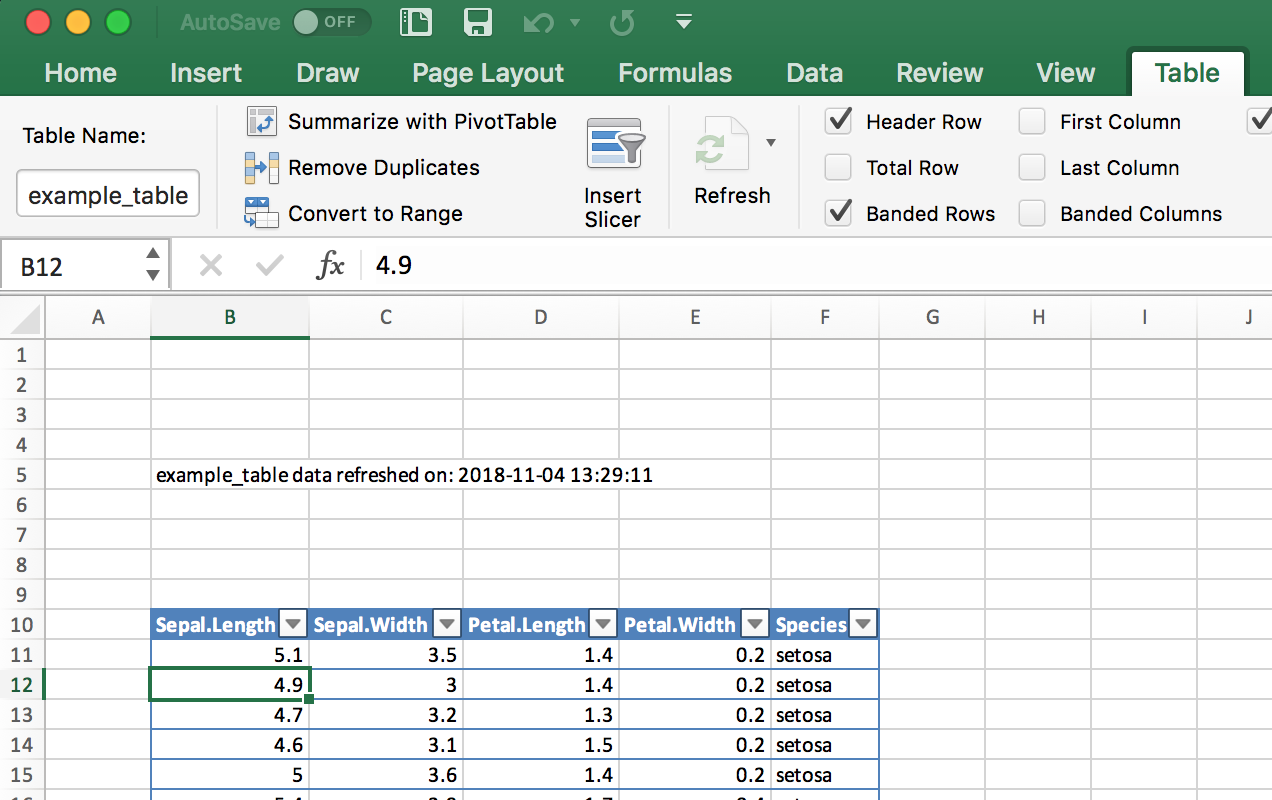
Vingette for openxlsx by installing openxlsx and running:
vignette(Introduction, package=openxlsx)
The readxl package is party of the Tidyverse and provides fast, simple
reading of Excel files: https://readxl.tidyverse.org/
The writexl package is a fast and lightweight (no dependencies)
package for writing Excel files:
https://cran.r-project.org/web/packages/writexl/index.html
You want to read a SAS data set into an R data frame.
The sas7bdat package supports reading SAS sas7bdat files into R.
library(haven)sas_movie_data<-read_sas("data/movies.sas7bdat")
SAS V7 and beyond all support the sas7bdat file format. The read_sas
function in haven supports reading the sas7bdat file format including
variable labels. If your SAS file has variable labels, when they are
inported into R they will be stored in the label attributes of the
data frame. These labels will not be printed by default. You can see the
labels by opening the data frame in R Studio, or by calling the
attributes Base R function on each column:
sapply(sas_movie_data,attributes)#> $Movie#> $Movie$label#> [1] "Movie"#>#>#> $Type#> $Type$label#> [1] "Type"#>#>#> $Rating#> $Rating$label#> [1] "Rating"#>#>#> $Year#> $Year$label#> [1] "Year"#>#>#> $Domestic__#> $Domestic__$label#> [1] "Domestic $"#>#> $Domestic__$format.sas#> [1] "F"#>#>#> $Worldwide__#> $Worldwide__$label#> [1] "Worldwide $"#>#> $Worldwide__$format.sas#> [1] "F"#>#>#> $Director#> $Director$label#> [1] "Director"
The sas7bdat package is much slower on large files than haven, but
it has more elaborate support for file attributes. If the SAS metadata
is important to you then you should investigate
sas7bdat::read.sas7bdat.
You want to read data from an HTML table on the Web.
Use the read_html and html_table functions in the rvest package.
To read all tables on the page, do the following:
library(rvest)library(magrittr)all_tables<-read_html("https://en.wikipedia.org/wiki/Aviation_accidents_and_incidents")%>%html_table(fill=TRUE,header=TRUE)
read_html puts all tables from the HTML document into the output list.
To pull a single table from that list, you can use the function
extract2 from the magrittr package:
out_table<-read_html("https://en.wikipedia.org/wiki/Aviation_accidents_and_incidents")%>%html_table(fill=TRUE,header=TRUE)%>%extract2(2)head(out_table)#> Year Deaths[52] # of incidents[53]#> 1 2017 399 101 [54]#> 2 2016 629 102#> 3 2015 898 123#> 4 2014 1,328 122#> 5 2013 459 138#> 6 2012 800 156
Note that the rvest and magrittr packages are both installed when
you run install.packages('tidyverse') They are not core tidyverse
packages, however, so you must explicitly load them, as shown here.
Web pages can contain several HTML tables. Calling read_html(url) then
piping that to html_table() reads all tables on the page and returns
them in a list. This can be useful for exploring a page, but it’s
annoying if you want just one specific table. In that case, use
extract2(n) to select the the _n_th table.
Two common parameters for the html_table function are fill=TRUE
which fills in missing values with NA, and header=TRUE which indicates
that the first row contains the header names.
The following example, loads all tables from the Wikipedia page entitled “World population”:
url<-'http://en.wikipedia.org/wiki/World_population'tbls<-read_html(url)%>%html_table(fill=TRUE,header=TRUE)
As it turns out, that page contains 24 tables (or things that
html_table thinks might be tables):
length(tbls)#> [1] 23
In this example we care only about the sixth table (which lists the
largest populations by country), so we can either access that element
using brackets: tbls[[6]] or we can pipe it into the extract2
function from the magrittr package:
library(magrittr)url<-'http://en.wikipedia.org/wiki/World_population'tbl<-read_html(url)%>%html_table(fill=TRUE,header=TRUE)%>%extract2(2)head(tbl,2)#> World population (millions, UN estimates)[10]#> 1 ##> 2 1#> World population (millions, UN estimates)[10]#> 1 Top ten most populous countries#> 2 China*#> World population (millions, UN estimates)[10]#> 1 2000#> 2 1,270#> World population (millions, UN estimates)[10]#> 1 2015#> 2 1,376#> World population (millions, UN estimates)[10]#> 1 2030*#> 2 1,416
In that table, columns 2 and 3 contain the country name and population, respectively:
tbl[,c(2,3)]#> World population (millions, UN estimates)[10]#> 1 Top ten most populous countries#> 2 China*#> 3 India#> 4 United States#> 5 Indonesia#> 6 Pakistan#> 7 Brazil#> 8 Nigeria#> 9 Bangladesh#> 10 Russia#> 11 Mexico#> 12 World total#> 13 Notes:\nChina = excludes Hong Kong and Macau\n2030 = Medium variant#> World population (millions, UN estimates)[10].1#> 1 2000#> 2 1,270#> 3 1,053#> 4 283#> 5 212#> 6 136#> 7 176#> 8 123#> 9 131#> 10 146#> 11 103#> 12 6,127#> 13 Notes:\nChina = excludes Hong Kong and Macau\n2030 = Medium variant
Right away, we can see problems with the data: the second row of the data has info that really belongs with the header. And China has * appended to its name. On the Wikipedia website, that was a footnote reference, but now it’s just a bit of unwanted text. Adding insult to injury, the population numbers have embedded commas, so you cannot easily convert them to raw numbers. All these problems can be solved by some string processing, but each problem adds at least one more step to the process.
This illustrates the main obstacle to reading HTML tables. HTML was designed for presenting information to people, not to computers. When you “scrape” information off an HTML page, you get stuff that’s useful to people but annoying to computers. If you ever have a choice, choose instead a computer-oriented data representation such as XML, JSON, or CSV.
The read_html(url) and html_table() functions are part of the
rvest package, which (by necessity) is large and complex. Any time you
pull data from a site designed for human readers, not machines, expect
that you will have to do post processing to clean up the bits and pieces
left messy by the machine.
See “Installing Packages from CRAN” for downloading and installing packages such as the rvest
package.
You are reading data from a file that has a complex or irregular structure.
Use the readLines function to read individual lines; then process
them as strings to extract data items.
Alternatively, use the scan function to read individual tokens and
use the argument what to describe the stream of tokens in your file.
The function can convert tokens into data and then assemble the data
into records.
Life would be simple and beautiful if all our data files were organized
into neat tables with cleanly delimited data. We could read those files
using one of the functions in the readr package and get on with
living.
Unfortunatly we don’t live in a land of rainbows and unicorn kisses.
You will eventually encounter a funky file format, and your job (suck it up, buttercup) is to read the file contents into R.
The read.table and read.csv functions are line-oriented and probably
won’t help. However, the readLines and scan functions are useful
here because they let you process the individual lines and even tokens
of the file.
The readLines function is pretty simple. It reads lines from a file
and returns them as a list of character strings:
lines<-readLines("input.txt")
You can limit the number of lines by using the n parameter, which
gives the number of maximum number of lines to be read:
lines<-readLines("input.txt",n=10)# Read 10 lines and stop
The scan function is much richer. It reads one token at a time and
handles it according to your instructions. The first argument is either
a filename or a connection (more on connections later). The second
argument is called what, and it describes the tokens that scan
should expect in the input file. The description is cryptic but quite
clever:
what=numeric(0)Interpret the next token as a number.
what=integer(0)Interpret the next token as an integer.
what=complex(0)Interpret the next token as complex number.
what=character(0)Interpret the next token as a character string.
what=logical(0)Interpret the next token as a logical value.
The scan function will apply the given pattern repeatedly until all
data is read.
Suppose your file is simply a sequence of numbers, like this:
2355.09 2246.73 1738.74 1841.01 2027.85
Use what=numeric(0) to say, “My file is a sequence of tokens, each of
which is a number”:
singles<-scan("./data/singles.txt",what=numeric(0))singles#> [1] 2355.09 2246.73 1738.74 1841.01 2027.85
A key feature of scan is that the what can be a list containing
several token types. The scan function will assume your file is a
repeating sequence of those types. Suppose your file contains triplets
of data, like this:
15-Oct-87 2439.78 2345.63 16-Oct-87 2396.21 2207.73
19-Oct-87 2164.16 1677.55 20-Oct-87 2067.47 1616.21
21-Oct-87 2081.07 1951.76
Use a list to tell scan that it should expect a repeating, three-token
sequence:
triples<-scan("./data/triples.txt",what=list(character(0),numeric(0),numeric(0)))triples#> [[1]]#> [1] "15-Oct-87" "16-Oct-87" "19-Oct-87" "20-Oct-87" "21-Oct-87"#>#> [[2]]#> [1] 2439.78 2396.21 2164.16 2067.47 2081.07#>#> [[3]]#> [1] 2345.63 2207.73 1677.55 1616.21 1951.76
Give names to the list elements, and scan will assign those names to
the data:
triples<-scan("./data/triples.txt",what=list(date=character(0),high=numeric(0),low=numeric(0)))triples#> $date#> [1] "15-Oct-87" "16-Oct-87" "19-Oct-87" "20-Oct-87" "21-Oct-87"#>#> $high#> [1] 2439.78 2396.21 2164.16 2067.47 2081.07#>#> $low#> [1] 2345.63 2207.73 1677.55 1616.21 1951.76
This can easily be turned into a data frame with the data.frame
command:
df_triples<-data.frame(triples)df_triples#> date high low#> 1 15-Oct-87 2439.78 2345.63#> 2 16-Oct-87 2396.21 2207.73#> 3 19-Oct-87 2164.16 1677.55#> 4 20-Oct-87 2067.47 1616.21#> 5 21-Oct-87 2081.07 1951.76
The scan function has many bells and whistles, but the following are
especially useful:
n=numberStop after reading this many tokens. (Default: stop at end of file.)
nlines=numberStop after reading this many input lines. (Default: stop at end of file.)
skip=numberNumber of input lines to skip before reading data.
na.strings=listA list of strings to be interpreted as NA.
Let’s use this recipe to read a dataset from StatLib, the repository of
statistical data and software maintained by Carnegie Mellon University.
Jeff Witmer contributed a dataset called wseries that shows the
pattern of wins and losses for every World Series since 1903. The
dataset is stored in an ASCII file with 35 lines of comments followed by
23 lines of data. The data itself looks like this:
1903  LWLlwwwW    1927  wwWW      1950  wwWW      1973  WLwllWW
1905  wLwWW       1928  WWww      1951  LWlwwW    1974  wlWWW
1906  wLwLwW      1929  wwLWW     1952  lwLWLww   1975  lwWLWlw
1907  WWww        1930  WWllwW    1953  WWllwW    1976  WWww
1908  wWLww       1931  LWwlwLW   1954  WWww      1977  WLwwlW

.
. (etc.)
.
The data is encoded as follows: L = loss at home, l = loss on the road, W = win at home, w = win on the road. The data appears in column order, not row order, which complicates our lives a bit.
Here is the R code for reading the raw data:
# Read the wseries dataset:# - Skip the first 35 lines# - Then read 23 lines of data# - The data occurs in pairs: a year and a pattern (char string)#world.series<-scan("http://lib.stat.cmu.edu/datasets/wseries",skip=35,nlines=23,what=list(year=integer(0),pattern=character(0)),)
The scan function returns a list, so we get a list with two elements:
year and pattern. The function reads from left to right, but the
dataset is organized by columns and so the years appear in a strange
order:
world.series$year#> [1] 1903 1927 1950 1973 1905 1928 1951 1974 1906 1929 1952 1975 1907 1930#> [15] 1953 1976 1908 1931 1954 1977 1909 1932 1955 1978 1910 1933 1956 1979#> [29] 1911 1934 1957 1980 1912 1935 1958 1981 1913 1936 1959 1982 1914 1937#> [43] 1960 1983 1915 1938 1961 1984 1916 1939 1962 1985 1917 1940 1963 1986#> [57] 1918 1941 1964 1987 1919 1942 1965 1988 1920 1943 1966 1989 1921 1944#> [71] 1967 1990 1922 1945 1968 1991 1923 1946 1969 1992 1924 1947 1970 1993#> [85] 1925 1948 1971 1926 1949 1972
We can fix that by sorting the list elements according to year:
perm<-order(world.series$year)world.series<-list(year=world.series$year[perm],pattern=world.series$pattern[perm])
Now the data appears in chronological order:
world.series$year#> [1] 1903 1905 1906 1907 1908 1909 1910 1911 1912 1913 1914 1915 1916 1917#> [15] 1918 1919 1920 1921 1922 1923 1924 1925 1926 1927 1928 1929 1930 1931#> [29] 1932 1933 1934 1935 1936 1937 1938 1939 1940 1941 1942 1943 1944 1945#> [43] 1946 1947 1948 1949 1950 1951 1952 1953 1954 1955 1956 1957 1958 1959#> [57] 1960 1961 1962 1963 1964 1965 1966 1967 1968 1969 1970 1971 1972 1973#> [71] 1974 1975 1976 1977 1978 1979 1980 1981 1982 1983 1984 1985 1986 1987#> [85] 1988 1989 1990 1991 1992 1993world.series$pattern#> [1] "LWLlwwwW" "wLwWW" "wLwLwW" "WWww" "wWLww" "WLwlWlw"#> [7] "WWwlw" "lWwWlW" "wLwWlLW" "wLwWw" "wwWW" "lwWWw"#> [13] "WWlwW" "WWllWw" "wlwWLW" "WWlwwLLw" "wllWWWW" "LlWwLwWw"#> [19] "WWwW" "LwLwWw" "LWlwlWW" "LWllwWW" "lwWLLww" "wwWW"#> [25] "WWww" "wwLWW" "WWllwW" "LWwlwLW" "WWww" "WWlww"#> [31] "wlWLLww" "LWwwlW" "lwWWLw" "WWwlw" "wwWW" "WWww"#> [37] "LWlwlWW" "WLwww" "LWwww" "WLWww" "LWlwwW" "LWLwwlw"#> [43] "LWlwlww" "WWllwLW" "lwWWLw" "WLwww" "wwWW" "LWlwwW"#> [49] "lwLWLww" "WWllwW" "WWww" "llWWWlw" "llWWWlw" "lwLWWlw"#> [55] "llWLWww" "lwWWLw" "WLlwwLW" "WLwww" "wlWLWlw" "wwWW"#> [61] "WLlwwLW" "llWWWlw" "wwWW" "wlWWLlw" "lwLLWww" "lwWWW"#> [67] "wwWLW" "llWWWlw" "wwLWLlw" "WLwllWW" "wlWWW" "lwWLWlw"#> [73] "WWww" "WLwwlW" "llWWWw" "lwLLWww" "WWllwW" "llWWWw"#> [79] "LWwllWW" "LWwww" "wlWWW" "LLwlwWW" "LLwwlWW" "WWlllWW"#> [85] "WWlww" "WWww" "WWww" "WWlllWW" "lwWWLw" "WLwwlW"
You want access to data stored in a MySQL database.
Install the RMySQL package on your computer.
Open a database connection using the DBI::dbConnect function.
Use dbGetQuery to initiate a SELECT and return the result sets.
Use dbDisconnect to terminate the database connection when you are
done.
This recipe requires that the RMySQL package be installed on your
computer. That package requires, in turn, the MySQL client software. If
the MySQL client software is not already installed and configured,
consult the MySQL documentation or your system administrator.
Use the dbConnect function to establish a connection to the MySQL
database. It returns a connection object which is used in subsequent
calls to RMySQL functions:
library(RMySQL)con<-dbConnect(drv=RMySQL::MySQL(),dbname="your_db_name",host="your.host.com",username="userid",password="pwd")
The username, password, and host parameters are the same parameters used
for accessing MySQL through the mysql client program. The example
given here shows them hard-coded into the dbConnect call. Actually,
that is an ill-advised practice. It puts your password in a plain text
document, creating a security problem. It also creates a major headache
whenever your password or host change, requiring you to hunt down the
hard-coded values. I strongly recommend using the security mechanism of
MySQL instead. Put those three parameters into your MySQL configuration
file, which is $HOME/.my.cnf on Unix and C:\my.cnf on Windows. Make
sure the file is unreadable by anyone except you. The file is delimited
into sections with markers such as [client]. Put the parameters into
the [client] section, so that your config file will contain something
like this:
[client]
user = userid
password = password
host = hostname
Once the parameters are defined in the config file, you no longer need
to supply them in the dbConnect call, which then becomes much simpler:
jal TODO - test this in anger
con<-dbConnect(dbConnect(drv=RMySQL::MySQL(),dbname="your_db_name",host="your.host.com")
Use the dbGetQuery function to submit your SQL to the database and
read the result sets. Doing so requires an open database connection:
sql<-"SELECT * from SurveyResults WHERE City = 'Chicago'"rows<-dbGetQuery(con,sql)
You are not restricted to SELECT statements. Any SQL that generates a
result set is OK. It is common to use CALL statements, for example, if
your SQL is encapsulated in stored procedures and those stored
procedures contain embedded SELECT statements.
Using dbGetQuery is convenient because it packages the result set into
a data frame and returns the data frame. This is the perfect
representation of an SQL result set. The result set is a tabular data
structure of rows and columns, and so is a data frame. The result set’s
columns have names given by the SQL SELECT statement, and R uses them
for naming the columns of the data frame.
After the first result set of data, MySQL can return a second result set
containing status information. You can choose to inspect the status or
ignore it, but you must read it. Otherwise, MySQL will complain that
there are unprocessed result sets and then halt. So call dbNextResult
if necessary:
if(dbMoreResults(con))dbNextResult(con)
Call dbGetQuery repeatedly to perform multiple queries, checking for
the result status after each call (and reading it, if necessary). When
you are done, close the database connection using dbDisconnect:
dbDisconnect(con)
Here is a complete session that reads and prints three rows from a
database of stock prices. The query selects the price of IBM stock for
the last three days of 2008. It assumes that the username, password, and
host are defined in the my.cnf file:
con<-dbConnect(MySQL(),client.flag=CLIENT_MULTI_RESULTS)sql<-paste("select * from DailyBar where Symbol = 'IBM'","and Day between '2008-12-29' and '2008-12-31'")rows<-dbGetQuery(con,sql)if(dbMoreResults(con)){dbNextResults(con)}dbDisconnect(con)(rows)
*TODO - format this so it looks like output, maybe? * TODO - do we need the dbMoreResults still? Symbol Day Next OpenPx HighPx LowPx ClosePx AdjClosePx 1 IBM 2008-12-29 2008-12-30 81.72 81.72 79.68 81.25 81.25 2 IBM 2008-12-30 2008-12-31 81.83 83.64 81.52 83.55 83.55 3 IBM 2008-12-31 2009-01-02 83.50 85.00 83.50 84.16 84.16 HistClosePx Volume OpenInt 1 81.25 6062600 NA 2 83.55 5774400 NA 3 84.16 6667700 NA
See “Installing Packages from CRAN” and the documentation for RMySQL, which contains more
details about configuring and using the package.
See “Accessing a Database with dbplyr” for information about how to get data from an SQL without actually writing SQL yourself.
R can read from several other RDBMS systems, including Oracle, Sybase, PostgreSQL, and SQLite. For more information, see the R Data Import/Export guide, which is supplied with the base distribution (“Viewing the Supplied Documentation”) and is also available on CRAN at http://cran.r-project.org/doc/manuals/R-data.pdf.
You want to access a database, but you’d rather not write SQL code in order to manipulate data and return results to R.
In addition to being a grammar of data manipulation, the tidyverse
package dplyr can, in in connection with the dbplyr package, turn
dplyr commands into SQL for you.
Let’s set up an example database using RSQLite and then we’ll connect
to it and use dplyr and the dbplyr backend to extract data.
Set up the example table by loading the msleep example data into an
in-memory SQLite database:
con<-DBI::dbConnect(RSQLite::SQLite(),":memory:")sleep_db<-copy_to(con,msleep,"sleep")
Now that we have a table in our database, we can create a reference to
it from R
sleep_table<-tbl(con,"sleep")
The sleep_table object is a type of pointer or alias to the table on
the database. However, dplyr will treat it like a regular tidyverse
tibble or data frame. So you can operate on it using dplyr and other R
commands. Let’s select all anaimals from the data who sleep less than 3
hours.
little_sleep<-sleep_table%>%select(name,genus,order,sleep_total)%>%filter(sleep_total<3)
The dbplyr backend does not go fetch the data when we do the above
commands. But it does build the query and get ready. To see the query
built by dplyr you can use show_query:
show_query(little_sleep)#> <SQL>#> SELECT *#> FROM (SELECT `name`, `genus`, `order`, `sleep_total`#> FROM `sleep`)#> WHERE (`sleep_total` < 3.0)
Then to bring the data back to your local machine use collect:
local_little_sleep<-collect(little_sleep)local_little_sleep#> # A tibble: 3 x 4#> name genus order sleep_total#> <chr> <chr> <chr> <dbl>#> 1 Horse Equus Perissodactyla 2.9#> 2 Giraffe Giraffa Artiodactyla 1.9#> 3 Pilot whale Globicephalus Cetacea 2.7
By using dplyr to access SQL databases by only writing dplyr commands, you can be more productive by not having to switch from one language to another and back. The alternative is to have large chunks of SQL code stored as text strings in the middle of an R script, or have the SQL in seperate files which are read in by R.
By allowing dplyr to transparently create the SQL in the background, the user is freed from having to maintain seperate SQL code to extract data.
The dbplyr package uses DBI to connect to your database, so you’ll need a DBI backend package for whichever database you want to access.
Some commonly used backend DBI packages are:
Uses the open database connectivity protocol to connect to many different databases. This is typically the best choice when connecting to Microsoft SQL Server. ODBC is typically straight forward on Windows machines but may require some considerable effort to get working in Linux or Mac.
For connecting to Postgres and Redshift.
For MySQL and MariaDB
Connecting to SQLite databases on disk or in memory.
For connections to Google’s BigQuery.
Each DBI backend package listed above is listed on CRAN and can be
installed with the typical install.packages('packagename') command.
For more information about connecting the databases with R & RStudio: https://db.rstudio.com/
For more detail on SQL translation in dbplyr, see the sql-translation
vignette at vignette("sql-translation") or
http://dbplyr.tidyverse.org/articles/sql-translation.html
You want to store one or more R objects in a file for later use, or you want to copy an R object from one machine to another.
Write the objects to a file using the save function:
save(tbl,t,file="myData.RData")
Read them back using the load function, either on your computer or on
any platform that supports R:
load("myData.RData")
The save function writes binary data. To save in an ASCII format, use
dput or dump instead:
dput(tbl,file="myData.txt")dump("tbl",file="myData.txt")# Note quotes around variable name
We’ve found ourselves with a large, complicated data object that we want
to load into other workspaces, or we may want to move R objects between
a Linux box and a Windows box. The load and save functions let us do
all this: save will store the object in a file that is portable across
machines, and load can read those files.
When you run load, it does not return your data per se; rather, it
creates variables in your workspace, loads your data into those
variables, and then returns the names of the variables (in a vector).
The first time you run load, you might be tempted to do this:
myData<-load("myData.RData")# Achtung! Might not do what you think
Let’s look at what myData is above:
myData#> [1] "tbl" "t"str(myData)#> chr [1:2] "tbl" "t"
This might be puzzling, because myData will not contain your data at
all. This can be perplexing and frustrating the first time.
The save function writes in a binary format to keep the file small.
Sometimes you want an ASCII format instead. When you submit a question
to a mailing list or to Stack Overflow, for example, including an ASCII
dump of the data lets others re-create your problem. In such cases use
dput or dump, which write an ASCII representation.
Be careful when you save and load objects created by a particular R
package. When you load the objects, R does not automatically load the
required packages, too, so it will not “understand” the object unless
you previously loaded the package yourself. For instance, suppose you
have an object called z created by the zoo package, and suppose we
save the object in a file called z.RData. The following sequence of
functions will create some confusion:
load("./data/z.RData")# Create and populate the z variableplot(z)# Does not plot as expected: zoo pkg not loaded
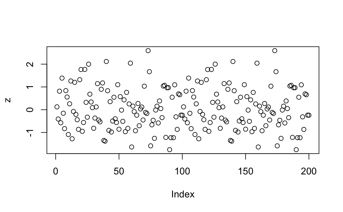
We should have loaded the zoo package before printing or plotting
any zoo objects, like this:
library(zoo)# Load the zoo package into memoryload("./data/z.RData")# Create and populate the z variableplot(z)# Ahhh. Now plotting works correctly
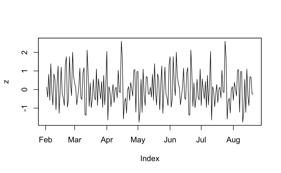
And you can see the resulting plot in Figure 4-2.
You can get pretty far in R just using vectors. That’s what Chapter 2 is all about. This chapter moves beyond vectors to recipes for matrices, lists, factors, data frames, and Tibbles (which are a special case of data frames). If you have preconceptions about data structures, I suggest you put them aside. R does data structures differently than many other languages.
If you want to study the technical aspects of R’s data structures, I suggest reading R in a Nutshell (O’Reilly) and the R Language Definition. The notes here are more informal. These are things we wish we’d known when we started using R.
Here are some key properties of vectors:
All elements of a vector must have the same type or, in R terminology, the same mode.
So v[2] refers to the second element of v.
So v[c(2,3)] is a subvector of v that consists of the second and
third elements.
Vectors have a names property, the same length as the vector itself,
that gives names to the elements:
+
v<-c(10,20,30)names(v)<-c("Moe","Larry","Curly")(v)#> Moe Larry Curly#> 10 20 30
Continuing the previous example: +
v["Larry"]#> Larry#> 20
Lists can contain elements of different types; in R terminology, list elements may have different modes. Lists can even contain other structured objects, such as lists and data frames; this allows you to create recursive data structures.
So lst[[2]] refers to the second element of lst. Note the double
square brackets. Double brackets means that R will return the element
as whatever type of element it is.
So lst[c(2,3)] is a sublist of lst that consists of the second and
third elements. Note the single square brackets. Single brackets means
that R will return the items in a list. If you pull a single element
with single brackets, like lst[2] R will return a list of length 1
with the first item containing the desired item.
JDL TODO: read Jenny Bryant’s description and think about clarifying this list business
Both lst[["Moe"]] and lst$Moe refer to the element named “Moe”.
Since lists are heterogeneous and since their elements can be retrieved by name, a list is like a dictionary or hash or lookup table in other programming languages (“Building a Name/Value Association List”). What’s surprising (and cool) is that in R, unlike most of those other programming languages, lists can also be indexed by position.
In R, every object has a mode, which indicates how it is stored in memory: as a number, as a character string, as a list of pointers to other objects, as a function, and so forth:
| Object | Example | Mode |
|---|---|---|
Number |
|
numeric |
Vector of numbers |
|
numeric |
Character string |
|
character |
Vector of character strings |
|
character |
Factor |
|
numeric |
List |
|
list |
Data frame |
|
list |
Function |
|
function |
The mode function gives us this information:
mode(3.1415)# Mode of a number#> [1] "numeric"mode(c(2.7182,3.1415))# Mode of a vector of numbers#> [1] "numeric"mode("Moe")# Mode of a character string#> [1] "character"mode(list("Moe","Larry","Curly"))# Mode of a list#> [1] "list"
A critical difference between a vector and a list can be summed up this way:
In a vector, all elements must have the same mode.
In a list, the elements can have different modes.
In R, every object also has a class, which defines its abstract type. The terminology is borrowed from object-oriented programming. A single number could represent many different things: a distance, a point in time, a weight. All those objects have a mode of “numeric” because they are stored as a number; but they could have different classes to indicate their interpretation.
For example, a Date object consists of a single number:
d<-as.Date("2010-03-15")mode(d)#> [1] "numeric"length(d)#> [1] 1
But it has a class of Date, telling us how to interpret that number;
namely, as the number of days since January 1, 1970:
class(d)#> [1] "Date"
R uses an object’s class to decide how to process the object. For
example, the generic function print has specialized versions (called
methods) for printing objects according to their class: data.frame,
Date, lm, and so forth. When you print an object, R calls the
appropriate print function according to the object’s class.
The quirky thing about scalars is their relationship to vectors. In some software, scalars and vectors are two different things. In R, they are the same thing: a scalar is simply a vector that contains exactly one element. In this book I often use the term “scalar”, but that’s just shorthand for “vector with one element.”
Consider the built-in constant pi. It is a scalar:
pi#> [1] 3.14
Since a scalar is a one-element vector, you can use vector functions on
pi:
length(pi)#> [1] 1
You can index it. The first (and only) element is π, of course:
pi[1]#> [1] 3.14
If you ask for the second element, there is none:
pi[2]#> [1] NA
In R, a matrix is just a vector that has dimensions. It may seem strange at first, but you can transform a vector into a matrix simply by giving it dimensions.
A vector has an attribute called dim, which is initially NULL, as
shown here:
A<-1:6dim(A)#> NULL(A)#> [1] 1 2 3 4 5 6
We give dimensions to the vector when we set its dim attribute. Watch
what happens when we set our vector dimensions to 2 × 3 and print it:
dim(A)<-c(2,3)(A)#> [,1] [,2] [,3]#> [1,] 1 3 5#> [2,] 2 4 6
Voilà! The vector was reshaped into a 2 × 3 matrix.
A matrix can be created from a list, too. Like a vector, a list has a
dim attribute, which is initially NULL:
B<-list(1,2,3,4,5,6)dim(B)#> NULL
If we set the dim attribute, it gives the list a shape:
dim(B)<-c(2,3)(B)#> [,1] [,2] [,3]#> [1,] 1 3 5#> [2,] 2 4 6
Voilà! We have turned this list into a 2 × 3 matrix.
The discussion of matrices can be generalized to 3-dimensional or even n-dimensional structures: just assign more dimensions to the underlying vector (or list). The following example creates a 3-dimensional array with dimensions 2 × 3 × 2:
D<-1:12dim(D)<-c(2,3,2)(D)#> , , 1#>#> [,1] [,2] [,3]#> [1,] 1 3 5#> [2,] 2 4 6#>#> , , 2#>#> [,1] [,2] [,3]#> [1,] 7 9 11#> [2,] 8 10 12
Note that R prints one “slice” of the structure at a time, since it’s not possible to print a 3-dimensional structure on a 2-dimensional medium.
It strikes us as very odd that we can turn a list into a matrix just by
giving the list a dim attribute. But wait; it gets stranger.
Recall that a list can be heterogeneous (mixed modes). We can start with a heterogeneous list, give it dimensions, and thus create a heterogeneous matrix. This code snippet creates a matrix that is a mix of numeric and character data:
C<-list(1,2,3,"X","Y","Z")dim(C)<-c(2,3)(C)#> [,1] [,2] [,3]#> [1,] 1 3 "Y"#> [2,] 2 "X" "Z"
To me this is strange because I ordinarily assume a matrix is purely numeric, not mixed. R is not that restrictive.
The possibility of a heterogeneous matrix may seem powerful and strangely fascinating. However, it creates problems when you are doing normal, day-to-day stuff with matrices. For example, what happens when the matrix C (above) is used in matrix multiplication? What happens if it is converted to a data frame? The answer is that odd things happen.
In this book, I generally ignore the pathological case of a heterogeneous matrix. I assume you’ve got simple, vanilla matrices. Some recipes involving matrices may work oddly (or not at all) if your matrix contains mixed data. Converting such a matrix to a vector or data frame, for instance, can be problematic (“Converting One Structured Data Type into Another”).
A factor looks like a character vector, but it has special properties. R keeps track of the unique values in a vector, and each unique value is called a level of the associated factor. R uses a compact representation for factors, which makes them efficient for storage in data frames. In other programming languages, a factor would be represented by a vector of enumerated values.
There are two key uses for factors:
A factor can represent a categorical variable. Categorical variables are used in contingency tables, linear regression, analysis of variance (ANOVA), logistic regression, and many other areas.
This is a technique for labeling or tagging your data items according to their group. See the Introduction to Data Transformations.
A data frame is powerful and flexible structure. Most serious R applications involve data frames. A data frame is intended to mimic a dataset, such as one you might encounter in SAS or SPSS.
A data frame is a tabular (rectangular) data structure, which means that it has rows and columns. It is not implemented by a matrix, however. Rather, a data frame is a list:
The elements of the list are vectors and/or factors.1
Those vectors and factors are the columns of the data frame.
The vectors and factors must all have the same length; in other words, all columns must have the same height.
The equal-height columns give a rectangular shape to the data frame.
The columns must have names.
Because a data frame is both a list and a rectangular structure, R provides two different paradigms for accessing its contents:
You can use list operators to extract columns from a data frame, such
as df[i], df[[i]], or df$name.
You can use matrix-like notation, such as df[i,j], df[i,], or
df[,j].
Your perception of a data frame likely depends on your background:
A data frame is a table of observations. Each row contains one observation. Each observation must contain the same variables. These variables are called columns, and you can refer to them by name. You can also refer to the contents by row number and column number, just as with a matrix.
A data frame is a table. The table resides entirely in memory, but you can save it to a flat file and restore it later. You needn’t declare the column types because R figures that out for you.
A data frame is like a worksheet, or perhaps a range within a worksheet. It is more restrictive, however, in that each column has a type.
A data frame is like a SAS dataset for which all the data resides in memory. R can read and write the data frame to disk, but the data frame must be in memory while R is processing it.
A data frame is a hybrid data structure, part matrix and part list. A column can contain numbers, character strings, or factors but not a mix of them. You can index the data frame just like you index a matrix. The data frame is also a list, where the list elements are the columns, so you can access columns by using list operators.
A data frame is a rectangular data structure. The columns are strongly typed, and each column must be numeric values, character strings, or a factor. Columns must have labels; rows may have labels. The table can be indexed by position, column name, and/or row name. It can also be accessed by list operators, in which case R treats the data frame as a list whose elements are the columns of the data frame.
You can put names and numbers into a data frame. It’s easy! A data frame is like a little database. Your staff will enjoy using data frames.`
A tibble is a modern reimagining of the data frame, introduced by Hadley Wickham in his Tidyverse packages. Most of the common functions you would use with data frames also work with Tibbles. However Tibbles typically do less than data frames and complain more. This idea of complaining and doing less may remind you of your least favorite coworker, however, we think tibbles will be one of your most favorite data structures. Doing less and complaining more can be a feature, not a bug.
Unlike data frames, tibbles do not:
Tibbles do not give you row numbers by default.
Tibbles do not coerce column names and surprise you with names different than you expected.
Tibbles don’t coerce your data into factors without you explictly asking for that.
Tibbles only recycle vectors of length 1.
In addition to basic data frame functionality, tibbles also do this:
Tibbles only print the top four rows and a bit of metadata by default.
Tibbles always return a tibble when subsetting.
Tibbles never do partial matching: if you want a column from a tibble you have to ask for it using its full name.
Tibbles complain more by giving you more warnings and chatty messages to make sure you understand what the software is doing.
All these extras are designed to give you fewer surprises and help you be more productive.
You want to append additional data items to a vector.
Use the vector constructor (c) to construct a vector with the
additional data items:
v<-c(1,2,3)newItems<-c(6,7,8)v<-c(v,newItems)v#> [1] 1 2 3 6 7 8
For a single item, you can also assign the new item to the next vector element. R will automatically extend the vector:
v[length(v)+1]<-42v#> [1] 1 2 3 6 7 8 42
If you ask us about appending a data item to a vector, we will likely suggest that maybe you shouldn’t.
R works best when you think about entire vectors, not single data items. Are you repeatedly appending items to a vector? If so, then you are probably working inside a loop. That’s OK for small vectors, but for large vectors your program will run slowly. The memory management in R works poorly when you repeatedly extend a vector by one element. Try to replace that loop with vector-level operations. You’ll write less code, and R will run much faster.
Nonetheless, one does occasionally need to append data to vectors. Our
experiments show that the most efficient way is to create a new vector
using the vector constructor (c) to join the old and new data. This
works for appending single elements or multiple elements:
v<-c(1,2,3)v<-c(v,4)# Append a single value to vv#> [1] 1 2 3 4w<-c(5,6,7,8)v<-c(v,w)# Append an entire vector to vv#> [1] 1 2 3 4 5 6 7 8
You can also append an item by assigning it to the position past the end of the vector, as shown in the Solution. In fact, R is very liberal about extending vectors. You can assign to any element and R will expand the vector to accommodate your request:
v<-c(1,2,3)# Create a vector of three elementsv[10]<-10# Assign to the 10th elementv# R extends the vector automatically#> [1] 1 2 3 NA NA NA NA NA NA 10
Note that R did not complain about the out-of-bounds subscript. It just extended the vector to the needed length, filling with NA.
R includes an append function that creates a new vector by appending
items to an existing vector. However, our experiments show that this
function runs more slowly than both the vector constructor and the
element assignment.
You want to insert one or more data items into a vector.
Despite its name, the append function inserts data into a vector by
using the after parameter, which gives the insertion point for the new
item or items:
v#> [1] 1 2 3 NA NA NA NA NA NA 10newvalues<-c(100,101)n<-2append(v,newvalues,after=n)#> [1] 1 2 100 101 3 NA NA NA NA NA NA 10
The new items will be inserted at the position given by after. This
example inserts 99 into the middle of a sequence:
append(1:10,99,after=5)#> [1] 1 2 3 4 5 99 6 7 8 9 10
The special value of after=0 means insert the new items at the head of
the vector:
append(1:10,99,after=0)#> [1] 99 1 2 3 4 5 6 7 8 9 10
The comments in “Appending Data to a Vector” apply here, too. If you are inserting single items into a vector, you might be working at the element level when working at the vector level would be easier to code and faster to run.
You want to understand the mysterious Recycling Rule that governs how R handles vectors of unequal length.
When you do vector arithmetic, R performs element-by-element operations. That works well when both vectors have the same length: R pairs the elements of the vectors and applies the operation to those pairs.
But what happens when the vectors have unequal lengths?
In that case, R invokes the Recycling Rule. It processes the vector element in pairs, starting at the first elements of both vectors. At a certain point, the shorter vector is exhausted while the longer vector still has unprocessed elements. R returns to the beginning of the shorter vector, “recycling” its elements; continues taking elements from the longer vector; and completes the operation. It will recycle the shorter-vector elements as often as necessary until the operation is complete.
It’s useful to visualize the Recycling Rule. Here is a diagram of two vectors, 1:6 and 1:3:
1:6 1:3
----- -----
1 1
2 2
3 3
4
5
6
Obviously, the 1:6 vector is longer than the 1:3 vector. If we try to add the vectors using (1:6) + (1:3), it appears that 1:3 has too few elements. However, R recycles the elements of 1:3, pairing the two vectors like this and producing a six-element vector:
1:6 1:3 (1:6) + (1:3)
----- ----- ---------------
1 1 2
2 2 4
3 3 6
4 5
5 7
6 9
Here is what you see in the R console:
(1:6)+(1:3)#> [1] 2 4 6 5 7 9
It’s not only vector operations that invoke the Recycling Rule;
functions can, too. The cbind function can create column vectors, such
as the following column vectors of 1:6 and 1:3. The two column have
different heights, of course:
r} cbind(1:6) cbind(1:3)
If we try binding these column vectors together into a two-column
matrix, the lengths are mismatched. The 1:3 vector is too short, so
cbind invokes the Recycling Rule and recycles the elements of 1:3:
cbind(1:6,1:3)#> [,1] [,2]#> [1,] 1 1#> [2,] 2 2#> [3,] 3 3#> [4,] 4 1#> [5,] 5 2#> [6,] 6 3
If the longer vector’s length is not a multiple of the shorter vector’s length, R gives a warning. That’s good, since the operation is highly suspect and there is likely a bug in your logic:
(1:6)+(1:5)# Oops! 1:5 is one element too short#> Warning in (1:6) + (1:5): longer object length is not a multiple of shorter#> object length#> [1] 2 4 6 8 10 7
Once you understand the Recycling Rule, you will realize that operations between a vector and a scalar are simply applications of that rule. In this example, the 10 is recycled repeatedly until the vector addition is complete:
(1:6)+10#> [1] 11 12 13 14 15 16
You have a vector of character strings or integers. You want R to treat them as a factor, which is R’s term for a categorical variable.
The factor function encodes your vector of discrete values into a
factor:
v<-c("dog","cat","mouse","rat","dog")f<-factor(v)# v can be a vector of strings or integersf#> [1] dog cat mouse rat dog#> Levels: cat dog mouse ratstr(f)#> Factor w/ 4 levels "cat","dog","mouse",..: 2 1 3 4 2
If your vector contains only a subset of possible values and not the entire universe, then include a second argument that gives the possible levels of the factor:
v<-c("dog","cat","mouse","rat","dog")f<-factor(v,levels=c("dog","cat","mouse","rat","horse"))f#> [1] dog cat mouse rat dog#> Levels: dog cat mouse rat horsestr(f)#> Factor w/ 5 levels "dog","cat","mouse",..: 1 2 3 4 1
In R, each possible value of a categorical variable is called a level. A vector of levels is called a factor. Factors fit very cleanly into the vector orientation of R, and they are used in powerful ways for processing data and building statistical models.
Most of the time, converting your categorical data into a factor is a
simple matter of calling the factor function, which identifies the
distinct levels of the categorical data and packs them into a factor:
f<-factor(c("Win","Win","Lose","Tie","Win","Lose"))f#> [1] Win Win Lose Tie Win Lose#> Levels: Lose Tie Win
Notice that when we printed the factor, f, R did not put quotes around
the values. They are levels, not strings. Also notice that when we
printed the factor, R also displayed the distinct levels below the
factor.
If your vector contains only a subset of all the possible levels, then R
will have an incomplete picture of the possible levels. Suppose you have
a string-valued variable wday that gives the day of the week on which
your data was observed:
wday<-c("Wed","Thu","Mon","Wed","Thu","Thu","Thu","Tue","Thu","Tue")f<-factor(wday)f#> [1] Wed Thu Mon Wed Thu Thu Thu Tue Thu Tue#> Levels: Mon Thu Tue Wed
R thinks that Monday, Thursday, Tuesday, and Wednesday are the only
possible levels. Friday is not listed. Apparently, the lab staff never
made observations on Friday, so R does not know that Friday is a
possible value. Hence you need to list the possible levels of wday
explicitly:
f<-factor(wday,c("Mon","Tue","Wed","Thu","Fri"))f#> [1] Wed Thu Mon Wed Thu Thu Thu Tue Thu Tue#> Levels: Mon Tue Wed Thu Fri
Now R understands that f is a factor with five possible levels. It
knows their correct order, too. It originally put Thursday before
Tuesday because it assumes alphabetical order by default.2 The explicit
second argument defines the correct order.
In many situations it is not necessary to call factor explicitly. When
an R function requires a factor, it usually converts your data to a
factor automatically. The table function, for instance, works only on
factors, so it routinely converts its inputs to factors without asking.
You must explicitly create a factor variable when you want to specify
the full set of levels or when you want to control the ordering of
levels.
When creating a data frame using base R functinos like data.frame the
default behavior for text fields is to turn them into factors. This has
caused grief and consternation for many R users over the years as often
we expect text fields to be imported simply as text, not factors.
Tibbles, part of the Tidyverse of tools, on the other hand, never
converts to factors by default.
See Recipe X-X to create a factor from continuous data.
You have several groups of data, with one vector for each group. You want to combine the vectors into one large vector and simultaneously create a parallel factor that identifies each value’s original group.
Create a list that contains the vectors. Use the stack function to
combine the list into a two-column data frame:
v1<-c(1,2,3)v2<-c(4,5,6)v3<-c(7,8,9)comb<-stack(list(v1=v1,v2=v2,v3=v3))# Combine 3 vectorscomb#> values ind#> 1 1 v1#> 2 2 v1#> 3 3 v1#> 4 4 v2#> 5 5 v2#> 6 6 v2#> 7 7 v3#> 8 8 v3#> 9 9 v3
The data frame’s columns are called values and ind. The first column
contains the data, and the second column contains the parallel factor.
Why in the world would you want to mash all your data into one big vector and a parallel factor? The reason is that many important statistical functions require the data in that format.
Suppose you survey freshmen, sophomores, and juniors regarding their
confidence level (“What percentage of the time do you feel confident in
school?”). Now you have three vectors, called freshmen, sophomores,
and juniors. You want to perform an ANOVA analysis of the differences
between the groups. The ANOVA function, aov, requires one vector with
the survey results as well as a parallel factor that identifies the
group. You can combine the groups using the stack function:
set.seed(2)n<-5freshmen<-sample(1:5,n,replace=TRUE,prob=c(.6,.2,.1,.05,.05))sophomores<-sample(1:5,n,replace=TRUE,prob=c(.05,.2,.6,.1,.05))juniors<-sample(1:5,n,replace=TRUE,prob=c(.05,.2,.55,.15,.05))comb<-stack(list(fresh=freshmen,soph=sophomores,jrs=juniors))(comb)#> values ind#> 1 1 fresh#> 2 2 fresh#> 3 1 fresh#> 4 1 fresh#> 5 5 fresh#> 6 5 soph#> 7 3 soph#> 8 4 soph#> 9 3 soph#> 10 3 soph#> 11 2 jrs#> 12 3 jrs#> 13 4 jrs#> 14 3 jrs#> 15 3 jrs
Now you can perform the ANOVA analysis on the two columns:
aov(values~ind,data=comb)#> Call:#> aov(formula = values ~ ind, data = comb)#>#> Terms:#> ind Residuals#> Sum of Squares 6.53 17.20#> Deg. of Freedom 2 12#>#> Residual standard error: 1.2#> Estimated effects may be unbalanced
When building the list we must provide tags for the list elements (the
tags are fresh, soph, and jrs in this example). Those tags are
required because stack uses them as the levels of the parallel factor.
You want to create and populate a list.
To create a list from individual data items, use the list function:
x<-c("a","b","c")y<-c(1,2,3)z<-"why be normal?"lst<-list(x,y,z)lst#> [[1]]#> [1] "a" "b" "c"#>#> [[2]]#> [1] 1 2 3#>#> [[3]]#> [1] "why be normal?"
Lists can be quite simple, such as this list of three numbers:
lst<-list(0.5,0.841,0.977)lst#> [[1]]#> [1] 0.5#>#> [[2]]#> [1] 0.841#>#> [[3]]#> [1] 0.977
When R prints the list, it identifies each list element by its position
([[1]], [[2]], [[3]]) and prints the element’s value (e.g.,
[1] 0.5) under its position.
More usefully, lists can, unlike vectors, contain elements of different modes (types). Here is an extreme example of a mongrel created from a scalar, a character string, a vector, and a function:
lst<-list(3.14,"Moe",c(1,1,2,3),mean)lst#> [[1]]#> [1] 3.14#>#> [[2]]#> [1] "Moe"#>#> [[3]]#> [1] 1 1 2 3#>#> [[4]]#> function (x, ...)#> UseMethod("mean")#> <bytecode: 0x7f8f0457ff88>#> <environment: namespace:base>
You can also build a list by creating an empty list and populating it. Here is our “mongrel” example built in that way:
lst<-list()lst[[1]]<-3.14lst[[2]]<-"Moe"lst[[3]]<-c(1,1,2,3)lst[[4]]<-meanlst#> [[1]]#> [1] 3.14#>#> [[2]]#> [1] "Moe"#>#> [[3]]#> [1] 1 1 2 3#>#> [[4]]#> function (x, ...)#> UseMethod("mean")#> <bytecode: 0x7f8f0457ff88>#> <environment: namespace:base>
List elements can be named. The list function lets you supply a name
for every element:
lst<-list(mid=0.5,right=0.841,far.right=0.977)lst#> $mid#> [1] 0.5#>#> $right#> [1] 0.841#>#> $far.right#> [1] 0.977
See the “Introduction” to this chapter for more about lists; see “Building a Name/Value Association List” for more about building and using lists with named elements.
You want to access list elements by position.
Use one of these ways. Here, lst is a list variable:
lst[[n]]Select the _n_th element from the list.
lst[c(n1, n2, ..., nk)]Returns a list of elements, selected by their positions.
Note that the first form returns a single element and the second returns a list.
Suppose we have a list of four integers, called years:
years<-list(1960,1964,1976,1994)years#> [[1]]#> [1] 1960#>#> [[2]]#> [1] 1964#>#> [[3]]#> [1] 1976#>#> [[4]]#> [1] 1994
We can access single elements using the double-square-bracket syntax:
years[[1]]
We can extract sublists using the single-square-bracket syntax:
years[c(1,2)]#> [[1]]#> [1] 1960#>#> [[2]]#> [1] 1964
This syntax can be confusing because of a subtlety: there is an
important difference between lst[[n]] and lst[n]. They are not the
same thing:
lst[[n]]This is an element, not a list. It is the _n_th element of lst.
lst[n]This is a list, not an element. The list contains one element, taken
from the _n_th element of lst. This is a special case of
lst[c(n1, n2, ..., nk)] in which we eliminated the c(…)
construct because there is only one n.
The difference becomes apparent when we inspect the structure of the result—one is a number; the other is a list:
class(years[[1]])#> [1] "numeric"class(years[1])#> [1] "list"
The difference becomes annoyingly apparent when we cat the value.
Recall that cat can print atomic values or vectors but complains about
printing structured objects:
cat(years[[1]],"\n")#> 1960cat(years[1],"\n")#> Error in cat(years[1], "\n"): argument 1 (type 'list') cannot be handled by 'cat'
We got lucky here because R alerted us to the problem. In other contexts, you might work long and hard to figure out that you accessed a sublist when you wanted an element, or vice versa.
You want to access list elements by their names.
Use one of these forms. Here, lst is a list variable:
lst[["name"]]Selects the element called name. Returns NULL if no element has that
name.
lst$nameSame as previous, just different syntax.
lst[c(name1, name2, ..., namek)]Returns a list built from the indicated elements of lst.
Note that the first two forms return an element whereas the third form returns a list.
Each element of a list can have a name. If named, the element can be selected by its name. This assignment creates a list of four named integers:
years<-list(Kennedy=1960,Johnson=1964,Carter=1976,Clinton=1994)
These next two expressions return the same value—namely, the element that is named “Kennedy”:
years[["Kennedy"]]#> [1] 1960years$Kennedy#> [1] 1960
The following two expressions return sublists extracted from years:
years[c("Kennedy","Johnson")]#> $Kennedy#> [1] 1960#>#> $Johnson#> [1] 1964years["Carter"]#> $Carter#> [1] 1976
Just as with selecting list elements by position
(“Selecting List Elements by Position”), there is an
important difference between lst[["name"]] and lst["name"]. They are
not the same:
lst[["name"]]This is an element, not a list.
lst["name"]This is a list, not an element. This is a special case of
lst[c(name1, name2, ..., namek)] in which we don’t need the
c(…) construct because there is only one name.
See “Selecting List Elements by Position” to access elements by position rather than by name.
You want to create a list that associates names and values — as would a dictionary, hash, or lookup table in another programming language.
The list function lets you give names to elements, creating an
association between each name and its value:
lst<-list(mid=0.5,right=0.841,far.right=0.977)lst#> $mid#> [1] 0.5#>#> $right#> [1] 0.841#>#> $far.right#> [1] 0.977
If you have parallel vectors of names and values, you can create an empty list and then populate the list by using a vectorized assignment statement:
values<-c(1,2,3)names<-c("a","b","c")lst<-list()lst[names]<-valueslst#> $a#> [1] 1#>#> $b#> [1] 2#>#> $c#> [1] 3
Each element of a list can be named, and you can retrieve list elements by name. This gives you a basic programming tool: the ability to associate names with values.
You can assign element names when you build the list. The list
function allows arguments of the form name=value:
lst<-list(far.left=0.023,left=0.159,mid=0.500,right=0.841,far.right=0.977)lst#> $far.left#> [1] 0.023#>#> $left#> [1] 0.159#>#> $mid#> [1] 0.5#>#> $right#> [1] 0.841#>#> $far.right#> [1] 0.977
One way to name the elements is to create an empty list and then populate it via assignment statements:
lst<-list()lst$far.left<-0.023lst$left<-0.159lst$mid<-0.500lst$right<-0.841lst$far.right<-0.977lst#> $far.left#> [1] 0.023#>#> $left#> [1] 0.159#>#> $mid#> [1] 0.5#>#> $right#> [1] 0.841#>#> $far.right#> [1] 0.977
Sometimes you have a vector of names and a vector of corresponding values:
values<-pnorm(-2:2)names<-c("far.left","left","mid","right","far.right")
You can associate the names and the values by creating an empty list and then populating it with a vectorized assignment statement:
lst<-list()lst[names]<-values
Once the association is made, the list can “translate” names into values through a simple list lookup:
cat("The left limit is",lst[["left"]],"\n")#> The left limit is 0.159cat("The right limit is",lst[["right"]],"\n")#> The right limit is 0.841for(nminnames(lst))cat("The",nm,"limit is",lst[[nm]],"\n")#> The far.left limit is 0.0228#> The left limit is 0.159#> The mid limit is 0.5#> The right limit is 0.841#> The far.right limit is 0.977
You want to remove an element from a list.
Assign NULL to the element. R will remove it from the list.
To remove a list element, select it by position or by name, and then
assign NULL to the selected element:
years<-list(Kennedy=1960,Johnson=1964,Carter=1976,Clinton=1994)years#> $Kennedy#> [1] 1960#>#> $Johnson#> [1] 1964#>#> $Carter#> [1] 1976#>#> $Clinton#> [1] 1994years[["Johnson"]]<-NULL# Remove the element labeled "Johnson"years#> $Kennedy#> [1] 1960#>#> $Carter#> [1] 1976#>#> $Clinton#> [1] 1994
You can remove multiple elements this way, too:
years[c("Carter","Clinton")]<-NULL# Remove two elementsyears#> $Kennedy#> [1] 1960
You want to flatten all the elements of a list into a vector.
Use the unlist function.
There are many contexts that require a vector. Basic statistical
functions work on vectors but not on lists, for example. If iq.scores
is a list of numbers, then we cannot directly compute their mean:
iq.scores<-list(rnorm(5,100,15))iq.scores#> [[1]]#> [1] 115.8 88.7 78.4 95.7 84.5mean(iq.scores)#> Warning in mean.default(iq.scores): argument is not numeric or logical:#> returning NA#> [1] NA
Instead, we must flatten the list into a vector using unlist and then
compute the mean of the result:
mean(unlist(iq.scores))#> [1] 92.6
Here is another example. We can cat scalars and vectors, but we cannot
cat a list:
cat(iq.scores,"\n")#> Error in cat(iq.scores, "\n"): argument 1 (type 'list') cannot be handled by 'cat'
One solution is to flatten the list into a vector before printing:
cat("IQ Scores:",unlist(iq.scores),"\n")#> IQ Scores: 116 88.7 78.4 95.7 84.5
Conversions such as this are discussed more fully in “Converting One Structured Data Type into Another”.
Your list contains NULL values. You want to remove them.
Suppose lst is a list some of whose elements are NULL. This
expression will remove the NULL elements:
lst<-list(1,NULL,2,3,NULL,4)lst#> [[1]]#> [1] 1#>#> [[2]]#> NULL#>#> [[3]]#> [1] 2#>#> [[4]]#> [1] 3#>#> [[5]]#> NULL#>#> [[6]]#> [1] 4lst[sapply(lst,is.null)]<-NULLlst#> [[1]]#> [1] 1#>#> [[2]]#> [1] 2#>#> [[3]]#> [1] 3#>#> [[4]]#> [1] 4
Finding and removing NULL elements from a list is surprisingly tricky.
The recipe above was written by one of the authors in a fit of
frustration after trying many other solutions that didn’t work. Here’s
how it works:
R calls sapply to apply the is.null function to every element of
the list.
sapply returns a vector of logical values that are TRUE wherever
the corresponding list element is NULL.
R selects values from the list according to that vector.
R assigns NULL to the selected items, removing them from the list.
The curious reader may be wondering how a list can contain NULL
elements, given that we remove elements by setting them to NULL
(“Removing an Element from a List”). The answer is
that we can create a list containing NULL elements:
lst<-list("Moe",NULL,"Curly")# Create list with NULL elementlst#> [[1]]#> [1] "Moe"#>#> [[2]]#> NULL#>#> [[3]]#> [1] "Curly"lst[sapply(lst,is.null)]<-NULL# Remove NULL element from listlst#> [[1]]#> [1] "Moe"#>#> [[2]]#> [1] "Curly"
In practice we might end up with NULL items in a list because of the results of a function we wrote to do something else.
See “Removing an Element from a List” for how to remove list elements.
You want to remove elements from a list according to a conditional test, such as removing elements that are negative or smaller than some threshold.
Build a logical vector based on the condition. Use the vector to select
list elements and then assign NULL to those elements. This assignment,
for example, removes all negative value from lst:
lst<-as.list(rnorm(7))lst#> [[1]]#> [1] -0.0281#>#> [[2]]#> [1] -0.366#>#> [[3]]#> [1] -1.12#>#> [[4]]#> [1] -0.976#>#> [[5]]#> [1] 1.12#>#> [[6]]#> [1] 0.324#>#> [[7]]#> [1] -0.568lst[lst<0]<-NULLlst#> [[1]]#> [1] 1.12#>#> [[2]]#> [1] 0.324
It’s worth noting that in the above example we use as.list instead of
list to create a list from the 7 random values created by rnorm(7).
The reason for this is that as.list will turn each element of a vector
into a list item. On the other hand, list would have given us a list
of length 1 where the first element was a vector containing 7 numbers:
list(rnorm(7))#> [[1]]#> [1] -1.034 -0.533 -0.981 0.823 -0.388 0.879 -2.178
This recipe is based on two useful features of R. First, a list can be
indexed by a logical vector. Wherever the vector element is TRUE, the
corresponding list element is selected. Second, you can remove a list
element by assigning NULL to it.
Suppose we want to remove elements from lst whose value is zero. We
construct a logical vector which identifies the unwanted values
(lst == 0). Then we select those elements from the list and assign
NULL to them:
lst[lst==0]<-NULL
This expression will remove NA values from the list:
lst[is.na(lst)]<-NULL
So far, so good. The problems arise when you cannot easily build the
logical vector. That often happens when you want to use a function that
cannot handle a list. Suppose you want to remove list elements whose
absolute value is less than 1. The abs function will not handle a
list, unfortunately:
lst[abs(lst)<1]<-NULL#> Error in abs(lst): non-numeric argument to mathematical function
The simplest solution is flattening the list into a vector by calling
unlist and then testing the vector:
lst#> [[1]]#> [1] 1.12#>#> [[2]]#> [1] 0.324lst[abs(unlist(lst))<1]<-NULLlst#> [[1]]#> [1] 1.12
A more elegant solution uses lapply (the list apply function) to apply
the function to every element of the list:
lst<-as.list(rnorm(5))lst#> [[1]]#> [1] 1.47#>#> [[2]]#> [1] 0.885#>#> [[3]]#> [1] 2.29#>#> [[4]]#> [1] 0.554#>#> [[5]]#> [1] 1.21lst[lapply(lst,abs)<1]<-NULLlst#> [[1]]#> [1] 1.47#>#> [[2]]#> [1] 2.29#>#> [[3]]#> [1] 1.21
Lists can hold complex objects, too, not just atomic values. Suppose
that mods is a list of linear models created by the lm function.
This expression will remove any model whose R2 value is less than
0.70:
x<-1:10y1<-2*x+rnorm(10,0,1)y2<-3*x+rnorm(10,0,8)result_list<-list(lm(x~y1),lm(x~y2))result_list[sapply(result_list,function(m)summary(m)$r.squared<0.7)]<-NULL
If we wanted to simply see the R2 values for each model, we could do the following:
sapply(result_list,function(m)summary(m)$r.squared)#> [1] 0.990 0.708
Using sapply (simple apply) will return a vector of results. If we had
used lapply we would have received a list in return:
lapply(result_list,function(m)summary(m)$r.squared)#> [[1]]#> [1] 0.99#>#> [[2]]#> [1] 0.708
It’s worth noting that if you face a situation like the one above, you might also explore the package called broom on CRAN. Broom is designed to take output of models and put the results in a tidy format that fits better in a tidy-style workflow.
You want to create a matrix and initialize it from given values.
Capture the data in a vector or list, and then use the matrix function
to shape the data into a matrix. This example shapes a vector into a 2 ×
3 matrix (i.e., two rows and three columns):
vec<-1:6matrix(vec,2,3)#> [,1] [,2] [,3]#> [1,] 1 3 5#> [2,] 2 4 6
The first argument of matrix is the data, the second argument is the
number of rows, and the third argument is the number of columns. Observe
that the matrix was filled column by column, not row by row.
It’s common to initialize an entire matrix to one value such as zero or
NA. If the first argument of matrix is a single value, then R will
apply the Recycling Rule and automatically replicate the value to fill
the entire matrix:
matrix(0,2,3)# Create an all-zeros matrix#> [,1] [,2] [,3]#> [1,] 0 0 0#> [2,] 0 0 0matrix(NA,2,3)# Create a matrix populated with NA#> [,1] [,2] [,3]#> [1,] NA NA NA#> [2,] NA NA NA
You can create a matrix with a one-liner, of course, but it becomes difficult to read:
mat<-matrix(c(1.1,1.2,1.3,2.1,2.2,2.3),2,3)mat#> [,1] [,2] [,3]#> [1,] 1.1 1.3 2.2#> [2,] 1.2 2.1 2.3
A common idiom in R is typing the data itself in a rectangular shape that reveals the matrix structure:
theData<-c(1.1,1.2,1.3,2.1,2.2,2.3)mat<-matrix(theData,2,3,byrow=TRUE)mat#> [,1] [,2] [,3]#> [1,] 1.1 1.2 1.3#> [2,] 2.1 2.2 2.3
Setting byrow=TRUE tells matrix that the data is row-by-row and not
column-by-column (which is the default). In condensed form, that
becomes:
mat<-matrix(c(1.1,1.2,1.3,2.1,2.2,2.3),2,3,byrow=TRUE)
Expressed this way, the reader quickly sees the two rows and three columns of data.
There is a quick-and-dirty way to turn a vector into a matrix: just assign dimensions to the vector. This was discussed in the “Introduction”. The following example creates a vanilla vector and then shapes it into a 2 × 3 matrix:
v<-c(1.1,1.2,1.3,2.1,2.2,2.3)dim(v)<-c(2,3)v#> [,1] [,2] [,3]#> [1,] 1.1 1.3 2.2#> [2,] 1.2 2.1 2.3
Personally, I find this more opaque than using matrix, especially
since there is no byrow option here.
You want to perform matrix operations such as transpose, matrix inversion, matrix multiplication, or constructing an identity matrix.
t(A)Matrix transposition of A
solve(A)Matrix inverse of A
A %*% BMatrix multiplication of A and B
diag(n)An n-by-n diagonal (identity) matrix
Recall that A*B is element-wise multiplication whereas A %*% B
is matrix multiplication.
All these functions return a matrix. Their arguments can be either matrices or data frames. If they are data frames then R will first convert them to matrices (although this is useful only if the data frame contains exclusively numeric values).
You want to assign descriptive names to the rows or columns of a matrix.
Every matrix has a rownames attribute and a colnames attribute.
Assign a vector of character strings to the appropriate attribute:
theData<-c(1.1,1.2,1.3,2.1,2.2,2.3,3.1,3.2,3.3)mat<-matrix(theData,3,3,byrow=TRUE)rownames(mat)<-c("rowname1","rowname2","rowname3")colnames(mat)<-c("colname1","colname2","colname3")mat#> colname1 colname2 colname3#> rowname1 1.1 1.2 1.3#> rowname2 2.1 2.2 2.3#> rowname3 3.1 3.2 3.3
R lets you assign names to the rows and columns of a matrix, which is
useful for printing the matrix. R will display the names if they are
defined, enhancing the readability of your output. Below we use the
quantmod library to pull stock prices for three tech stocks. Then we
calculate daily returns and create a correlation matrix of the daily
returns of Apple, Microsoft, and Google stock. No need to worry about
the details here, unless stocks are your thing. We’re just creating some
real-world data for illustration:
library("quantmod")#> Loading required package: xts#> Loading required package: zoo#>#> Attaching package: 'zoo'#> The following objects are masked from 'package:base':#>#> as.Date, as.Date.numeric#>#> Attaching package: 'xts'#> The following objects are masked from 'package:dplyr':#>#> first, last#> Loading required package: TTR#> Version 0.4-0 included new data defaults. See ?getSymbols.getSymbols(c("AAPL","MSFT","GOOG"),auto.assign=TRUE)#> 'getSymbols' currently uses auto.assign=TRUE by default, but will#> use auto.assign=FALSE in 0.5-0. You will still be able to use#> 'loadSymbols' to automatically load data. getOption("getSymbols.env")#> and getOption("getSymbols.auto.assign") will still be checked for#> alternate defaults.#>#> This message is shown once per session and may be disabled by setting#> options("getSymbols.warning4.0"=FALSE). See ?getSymbols for details.#>#> WARNING: There have been significant changes to Yahoo Finance data.#> Please see the Warning section of '?getSymbols.yahoo' for details.#>#> This message is shown once per session and may be disabled by setting#> options("getSymbols.yahoo.warning"=FALSE).#> [1] "AAPL" "MSFT" "GOOG"cor_mat<-cor(cbind(periodReturn(AAPL,period="daily",subset="2017"),periodReturn(MSFT,period="daily",subset="2017"),periodReturn(GOOG,period="daily",subset="2017")))cor_mat#> daily.returns daily.returns.1 daily.returns.2#> daily.returns 1.000 0.438 0.489#> daily.returns.1 0.438 1.000 0.619#> daily.returns.2 0.489 0.619 1.000
In this form, the matrix output’s interpretation is not self-evident.The
columns are named daily.returns.X because before we bound the columns
together with cbind they were each named daily.returns. R then
helped us manage the naming clash by appending .1 to the second column
and .2 to the third.
The default naming does not tell us which column came from which stock. So we’ll define names for the rows and columns, then R will annotate the matrix output with the names:
colnames(cor_mat)<-c("AAPL","MSFT","GOOG")rownames(cor_mat)<-c("AAPL","MSFT","GOOG")cor_mat#> AAPL MSFT GOOG#> AAPL 1.000 0.438 0.489#> MSFT 0.438 1.000 0.619#> GOOG 0.489 0.619 1.000
Now the reader knows at a glance which rows and columns apply to which stocks.
Another advantage of naming rows and columns is that you can refer to matrix elements by those names:
cor_mat["MSFT","GOOG"]# What is the correlation between MSFT and GOOG?#> [1] 0.619
You want to select a single row or a single column from a matrix.
The solution depends on what you want. If you want the result to be a simple vector, just use normal indexing:
mat[1,]# First row#> colname1 colname2 colname3#> 1.1 1.2 1.3mat[,3]# Third column#> rowname1 rowname2 rowname3#> 1.3 2.3 3.3
If you want the result to be a one-row matrix or a one-column matrix,
then include the drop=FALSE argument:
mat[1,,drop=FALSE]# First row in a one-row matrix#> colname1 colname2 colname3#> rowname1 1.1 1.2 1.3mat[,3,drop=FALSE]# Third column in a one-column matrix#> colname3#> rowname1 1.3#> rowname2 2.3#> rowname3 3.3
Normally, when you select one row or column from a matrix, R strips off the dimensions. The result is a dimensionless vector:
mat[1,]#> colname1 colname2 colname3#> 1.1 1.2 1.3mat[,3]#> rowname1 rowname2 rowname3#> 1.3 2.3 3.3
When you include the drop=FALSE argument, however, R retains the
dimensions. In that case, selecting a row returns a row vector (a 1 ×
n matrix):
mat[1,,drop=FALSE]#> colname1 colname2 colname3#> rowname1 1.1 1.2 1.3
Likewise, selecting a column with drop=FALSE returns a column vector
(an n × 1 matrix):
mat[,3,drop=FALSE]#> colname3#> rowname1 1.3#> rowname2 2.3#> rowname3 3.3
Your data is organized by columns, and you want to assemble it into a data frame.
If your data is captured in several vectors and/or factors, use the
data.frame function to assemble them into a data frame:
v1<-1:5v2<-6:10v3<-c("A","B","C","D","E")f1<-factor(c("a","a","a","b","b"))df<-data.frame(v1,v2,v3,f1)df#> v1 v2 v3 f1#> 1 1 6 A a#> 2 2 7 B a#> 3 3 8 C a#> 4 4 9 D b#> 5 5 10 E b
If your data is captured in a list that contains vectors and/or
factors, use instead as.data.frame:
list.of.vectors<-list(v1=v1,v2=v2,v3=v3,f1=f1)df2<-as.data.frame(list.of.vectors)df2#> v1 v2 v3 f1#> 1 1 6 A a#> 2 2 7 B a#> 3 3 8 C a#> 4 4 9 D b#> 5 5 10 E b
A data frame is a collection of columns, each of which corresponds to an observed variable (in the statistical sense, not the programming sense). If your data is already organized into columns, then it’s easy to build a data frame.
The data.frame function can construct a data frame from vectors, where
each vector is one observed variable. Suppose you have two numeric
predictor variables, one categorical predictor variable, and one
response variable. The data.frame function can create a data frame
from your vectors.
pred1<-rnorm(10)pred2<-rnorm(10,1,2)pred3<-sample(c("AM","PM"),10,replace=TRUE)resp<-2.1+pred1*.3+pred2*.9df<-data.frame(pred1,pred2,pred3,resp)df#> pred1 pred2 pred3 resp#> 1 -0.117 -0.0196 AM 2.05#> 2 -1.133 0.1529 AM 1.90#> 3 0.632 3.8004 AM 5.71#> 4 0.188 4.5922 AM 6.29#> 5 0.892 1.8556 AM 4.04#> 6 -1.224 2.8140 PM 4.27#> 7 0.174 0.4908 AM 2.59#> 8 -0.689 -0.1335 PM 1.77#> 9 1.204 -0.0482 AM 2.42#> 10 0.697 2.2268 PM 4.31
Notice that data.frame takes the column names from your program
variables. You can override that default by supplying explicit column
names:
df<-data.frame(p1=pred1,p2=pred2,p3=pred3,r=resp)head(df,3)#> p1 p2 p3 r#> 1 -0.117 -0.0196 AM 2.05#> 2 -1.133 0.1529 AM 1.90#> 3 0.632 3.8004 AM 5.71
As illustrated above, your data may be organized into vectors but those
vectors are held in a list, not individual program variables. Use the
as.data.frame function to create a data frame from the list of
vectors.
If you’d rather have a tibble (a.k.a tidy data frame) instead of a data
frame, then use the function as_tibble instead of data.frame.
However, note that as_tibble is designed to operate on a list, matrix,
data.frame, or table. So we can just wrap our vectors in a list
function before we call as_tibble:
tib<-as_tibble(list(p1=pred1,p2=pred2,p3=pred3,r=resp))tib#> # A tibble: 10 x 4#> p1 p2 p3 r#> <dbl> <dbl> <chr> <dbl>#> 1 -0.117 -0.0196 AM 2.05#> 2 -1.13 0.153 AM 1.90#> 3 0.632 3.80 AM 5.71#> 4 0.188 4.59 AM 6.29#> 5 0.892 1.86 AM 4.04#> 6 -1.22 2.81 PM 4.27#> # ... with 4 more rows
One subtle difference between a data.frame object and a tibble is
that when using the data.frame function to create a data.frame R
will coerce character values into factors by default. On the other hand,
as_tibble does not convert characters to factors. If you look at the
last two code examples above, you’ll see column p3 is of type chr in
the tibble example and type fctr in the data.frame example. This
difference is something you should be aware of as it can be maddeningly
frustrating to debug an issue caused by this subtle difference.
Your data is organized by rows, and you want to assemble it into a data frame.
Store each row in a one-row data frame. Store the one-row data frames in
a list. Use rbind and do.call to bind the rows into one, large data
frame:
r1<-data.frame(a=1,b=2,c="a")r2<-data.frame(a=3,b=4,c="b")r3<-data.frame(a=5,b=6,c="c")obs<-list(r1,r2,r3)df<-do.call(rbind,obs)df#> a b c#> 1 1 2 a#> 2 3 4 b#> 3 5 6 c
Here, obs is a list of one-row data frames. But notice that column c
is a factor, not a character.
Data often arrives as a collection of observations. Each observation is a record or tuple that contains several values, one for each observed variable. The lines of a flat file are usually like that: each line is one record, each record contains several columns, and each column is a different variable (see “Reading Files with a Complex Structure”). Such data is organized by observation, not by variable. In other words, you are given rows one at a time rather than columns one at a time.
Each such row might be stored in several ways. One obvious way is as a vector. If you have purely numerical data, use a vector.
However, many datasets are a mixture of numeric, character, and categorical data, in which case a vector won’t work. I recommend storing each such heterogeneous row in a one-row data frame. (You could store each row in a list, but this recipe gets a little more complicated.)
We need to bind together those rows into a data frame. That’s what the
rbind function does. It binds its arguments in such a way that each
argument becomes one row in the result. If we rbind the first two
observations, for example, we get a two-row data frame:
rbind(obs[[1]],obs[[2]])#> a b c#> 1 1 2 a#> 2 3 4 b
We want to bind together every observation, not just the first two, so
we tap into the vector processing of R. The do.call function will
expand obs into one, long argument list and call rbind with that
long argument list:
do.call(rbind,obs)#> a b c#> 1 1 2 a#> 2 3 4 b#> 3 5 6 c
The result is a data frame built from our rows of data.
Sometimes, for reasons beyond your control, the rows of your data are
stored in lists rather than one-row data frames. You may be dealing with
rows returned by a database package, for example. In that case, obs
will be a list of lists, not a list of data frames. We first transform
the rows into data frames using the Map function and then apply this
recipe:
l1<-list(a=1,b=2,c="a")l2<-list(a=3,b=4,c="b")l3<-list(a=5,b=6,c="c")obs<-list(l1,l2,l3)df<-do.call(rbind,Map(as.data.frame,obs))df#> a b c#> 1 1 2 a#> 2 3 4 b#> 3 5 6 c
This recipe works also if your observations are stored in vectors rather than one-row data frames. But with vectors, all elements have to be of the same data type. Though R will happily coerce integers into floats on the fly:
r1<-1:3r2<-6:8r3<-rnorm(3)obs<-list(r1,r2,r3)df<-do.call(rbind,obs)df#> [,1] [,2] [,3]#> [1,] 1.000 2.000 3.0#> [2,] 6.000 7.000 8.0#> [3,] -0.945 -0.547 1.6
Note the factor trap mentioned in the example above. If you would rather
get characters instead of factors, you have a couple of options. One is
to set the stringsAsFactors parameter to FALSE when data.frame is
called:
data.frame(a=1,b=2,c="a",stringsAsFactors=FALSE)#> a b c#> 1 1 2 a
Of course if you inherited your data and it’s already in a data frame
with factors, you can convert all factors in a data.frame to
characters using this bonus recipe:
## same set up as in the previous examples l1 <- list( a=1, b=2, c='a' ) l2 <- list( a=3, b=4, c='b' ) l3 <- list( a=5, b=6, c='c' ) obs <- list(l1, l2, l3) df <- do.call(rbind,Map(as.data.frame,obs)) # yes, you could use stringsAsFactors=FALSE above, but we're assuming the data.frame # came to you with factors already i <- sapply(df, is.factor) ## determine which columns are factors df[i] <- lapply(df[i], as.character) ## turn only the factors to characters df
Keep in mind that if you use a tibble instead of a data.frame then
characters will not be forced into factors by default.
See “Initializing a Data Frame from Column Data” if your data is organized by columns, not
rows.
See Recipe X-X to learn more about do.call.
You want to append one or more new rows to a data frame.
Create a second, temporary data frame containing the new rows. Then use
the rbind function to append the temporary data frame to the original
data frame.
Suppose we want to append a new row to our data frame of Chicago-area cities. First, we create a one-row data frame with the new data:
newRow<-data.frame(city="West Dundee",county="Kane",state="IL",pop=5428)
Next, we use the rbind function to append that one-row data frame to
our existing data frame:
library(tidyverse)suburbs<-read_csv("./data/suburbs.txt")#> Parsed with column specification:#> cols(#> city = col_character(),#> county = col_character(),#> state = col_character(),#> pop = col_double()#> )suburbs2<-rbind(suburbs,newRow)suburbs2#> # A tibble: 18 x 4#> city county state pop#> <chr> <chr> <chr> <dbl>#> 1 Chicago Cook IL 2853114#> 2 Kenosha Kenosha WI 90352#> 3 Aurora Kane IL 171782#> 4 Elgin Kane IL 94487#> 5 Gary Lake(IN) IN 102746#> 6 Joliet Kendall IL 106221#> # ... with 12 more rows
The rbind function tells R that we are appending a new row to
suburbs, not a new column. It may be obvious to you that newRow is a
row and not a column, but it is not obvious to R. (Use the cbind
function to append a column.)
One word of caution. The new row must use the same column names as the
data frame. Otherwise, rbind will fail.
We can combine these two steps into one, of course:
suburbs3<-rbind(suburbs,data.frame(city="West Dundee",county="Kane",state="IL",pop=5428))
We can even extend this technique to multiple new rows because rbind
allows multiple arguments:
suburbs4<-rbind(suburbs,data.frame(city="West Dundee",county="Kane",state="IL",pop=5428),data.frame(city="East Dundee",county="Kane",state="IL",pop=2955))
It’s worth noting that in the examples above we seamlessly comingled
tibbles and data frames because we used the tidy function read_csv
which produces tibbles. And note that the data frames contain factors
while the tibbles do not:
str(suburbs)#> Classes 'tbl_df', 'tbl' and 'data.frame': 17 obs. of 4 variables:#> $ city : chr "Chicago" "Kenosha" "Aurora" "Elgin" ...#> $ county: chr "Cook" "Kenosha" "Kane" "Kane" ...#> $ state : chr "IL" "WI" "IL" "IL" ...#> $ pop : num 2853114 90352 171782 94487 102746 ...#> - attr(*, "spec")=#> .. cols(#> .. city = col_character(),#> .. county = col_character(),#> .. state = col_character(),#> .. pop = col_double()#> .. )str(newRow)#> 'data.frame': 1 obs. of 4 variables:#> $ city : Factor w/ 1 level "West Dundee": 1#> $ county: Factor w/ 1 level "Kane": 1#> $ state : Factor w/ 1 level "IL": 1#> $ pop : num 5428
When this inputs to rbind are a mix of data.frame objects and
tibble objects, the result will be the type of object passed to the
first argument of rbind. So this would produce a tibble:
rbind(some_tibble,some_data.frame)
While this would produce a data.frame:
rbind(some_data.frame,some_tibble)
You are building a data frame, row by row. You want to preallocate the space instead of appending rows incrementally.
Create a data frame from generic vectors and factors using the functions
numeric(n) and`character(n)`:
n<-5df<-data.frame(colname1=numeric(n),colname2=character(n))
Here, n is the number of rows needed for the data frame.
Theoretically, you can build a data frame by appending new rows, one by one. That’s OK for small data frames, but building a large data frame in that way can be tortuous. The memory manager in R works poorly when one new row is repeatedly appended to a large data structure. Hence your R code will run very slowly.
One solution is to preallocate the data frame, assuming you know the required number of rows. By preallocating the data frame once and for all, you sidestep problems with the memory manager.
Suppose you want to create a data frame with 1,000,000 rows and three
columns: two numeric and one character. Use the numeric and
character functions to preallocate the columns; then join them
together using data.frame:
n<-1000000df<-data.frame(dosage=numeric(n),lab=character(n),response=numeric(n),stringsAsFactors=FALSE)str(df)#> 'data.frame': 1000000 obs. of 3 variables:#> $ dosage : num 0 0 0 0 0 0 0 0 0 0 ...#> $ lab : chr "" "" "" "" ...#> $ response: num 0 0 0 0 0 0 0 0 0 0 ...
Now you have a data frame with the correct dimensions, 1,000,000 × 3, waiting to receive its contents.
Notice in the example above we set stringsAsFactors=FALSE so that R
would not coerce the character field into factors. Data frames can
contain factors, but preallocating a factor is a little trickier. You
can’t simply call factor(n). You need to specify the factor’s levels
because you are creating it. Continuing our example, suppose you want
the lab column to be a factor, not a character string, and that the
possible levels are NJ, IL, and CA. Include the levels in the
column specification, like this:
n<-1000000df<-data.frame(dosage=numeric(n),lab=factor(n,levels=c("NJ","IL","CA")),response=numeric(n))str(df)#> 'data.frame': 1000000 obs. of 3 variables:#> $ dosage : num 0 0 0 0 0 0 0 0 0 0 ...#> $ lab : Factor w/ 3 levels "NJ","IL","CA": NA NA NA NA NA NA NA NA NA NA ...#> $ response: num 0 0 0 0 0 0 0 0 0 0 ...
You want to select columns from a data frame according to their position.
To select a single column, use this list operator:
df[[n]]Returns one column—specifically, the nth column of df.
To select one or more columns and package them in a data frame, use the following sublist expressions:
df[n]Returns a data frame consisting solely of the nth column of df.
df[c(n1, n2, ..., nk)]Returns a data frame built from the columns in positions n1,
n2, …, nk of df.
You can use matrix-style subscripting to select one or more columns:
df[, n]Returns the nth column (assuming that n contains exactly one value).
df[,c(n1, n2, ..., nk)]Returns a data frame built from the columns in positions n1, n2, …, nk.
Note that the matrix-style subscripting can return two different data types (either column or data frame) depending upon whether you select one column or multiple columns.
Or you can use the dplyr package from the Tidyverse and pass column
numbers to the select function to get back a tibble.
df %>% select(n1, n2, ..., nk)
There are a bewildering number of ways to select columns from a data frame. The choices can be confusing until you understand the logic behind the alternatives. As you read this explanation, notice how a slight change in syntax—a comma here, a double-bracket there—changes the meaning of the expression.
Let’s play with the population data for the 16 largest cities in the Chicago metropolitan area:
suburbs<-read_csv("./data/suburbs.txt")#> Parsed with column specification:#> cols(#> city = col_character(),#> county = col_character(),#> state = col_character(),#> pop = col_double()#> )suburbs#> # A tibble: 17 x 4#> city county state pop#> <chr> <chr> <chr> <dbl>#> 1 Chicago Cook IL 2853114#> 2 Kenosha Kenosha WI 90352#> 3 Aurora Kane IL 171782#> 4 Elgin Kane IL 94487#> 5 Gary Lake(IN) IN 102746#> 6 Joliet Kendall IL 106221#> # ... with 11 more rows
So right off the bat we can see this is a tibble. Subsetting and selecting in tibbles works very much like base R data frames. So the recipes below can work on either data structure.
Use simple list notation to select exactly one column, such as the first column:
suburbs[[1]]#> [1] "Chicago" "Kenosha" "Aurora"#> [4] "Elgin" "Gary" "Joliet"#> [7] "Naperville" "Arlington Heights" "Bolingbrook"#> [10] "Cicero" "Evanston" "Hammond"#> [13] "Palatine" "Schaumburg" "Skokie"#> [16] "Waukegan" "West Dundee"
The first column of suburbs is a vector, so that’s what suburbs[[1]]
returns: a vector. If the first column were a factor, we’d get a factor.
The result differs when you use the single-bracket notation, as in
suburbs[1] or suburbs[c(1,3)]. You still get the requested columns,
but R wraps them in a data frame. This example returns the first column
wrapped in a data frame:
suburbs[1]#> # A tibble: 17 x 1#> city#> <chr>#> 1 Chicago#> 2 Kenosha#> 3 Aurora#> 4 Elgin#> 5 Gary#> 6 Joliet#> # ... with 11 more rows
Another option, using the dplyr package from the Tidyverse, is to pipe
the data into a select statement: ** JAL note: both select statements
below are patch with dplyr:: issue with MASS not unloading?
suburbs%>%dplyr::select(1)#> # A tibble: 17 x 1#> city#> <chr>#> 1 Chicago#> 2 Kenosha#> 3 Aurora#> 4 Elgin#> 5 Gary#> 6 Joliet#> # ... with 11 more rows
You can, of course, use select from the dplyr package to pull more
than one column:
suburbs%>%dplyr::select(1,4)#> # A tibble: 17 x 2#> city pop#> <chr> <dbl>#> 1 Chicago 2853114#> 2 Kenosha 90352#> 3 Aurora 171782#> 4 Elgin 94487#> 5 Gary 102746#> 6 Joliet 106221#> # ... with 11 more rows
The next example returns the first and third columns as a data frame:
suburbs[c(1,3)]#> # A tibble: 17 x 2#> city state#> <chr> <chr>#> 1 Chicago IL#> 2 Kenosha WI#> 3 Aurora IL#> 4 Elgin IL#> 5 Gary IN#> 6 Joliet IL#> # ... with 11 more rows
A major source of confusion is that suburbs[[1]] and suburbs[1] look
similar but produce very different results:
suburbs[[1]]This returns one column.
suburbs[1]This returns a data frame, and the data frame contains exactly one
column. This is a special case of df[c(n1,n2, ..., nk)]. We don’t
need the c(...) construct because there is only one n.
The point here is that “one column” is different from “a data frame that contains one column.” The first expression returns a column, so it’s a vector or a factor. The second expression returns a data frame, which is different.
R lets you use matrix notation to select columns, as shown in the Solution. But an odd quirk can bite you: you might get a column or you might get a data frame, depending upon many subscripts you use. In the simple case of one index you get a column, like this:
suburbs[,1]#> # A tibble: 17 x 1#> city#> <chr>#> 1 Chicago#> 2 Kenosha#> 3 Aurora#> 4 Elgin#> 5 Gary#> 6 Joliet#> # ... with 11 more rows
But using the same matrix-style syntax with multiple indexes returns a data frame:
suburbs[,c(1,4)]#> # A tibble: 17 x 2#> city pop#> <chr> <dbl>#> 1 Chicago 2853114#> 2 Kenosha 90352#> 3 Aurora 171782#> 4 Elgin 94487#> 5 Gary 102746#> 6 Joliet 106221#> # ... with 11 more rows
This creates a problem. Suppose you see this expression in some old R script:
df[,vec]
Quick, does that return a column or a data frame? Well, it depends. If
vec contains one value then you get a column; otherwise, you get a
data frame. You cannot tell from the syntax alone.
To avoid this problem, you can include drop=FALSE in the subscripts;
this forces R to return a data frame:
df[,vec,drop=FALSE]
Now there is no ambiguity about the returned data structure. It’s a data frame.
When all is said and done, using matrix notation to select columns from
data frames is not the best procedure. It’s a good idea to instead use
the list operators described previously. They just seem clearer. Or you
can use the functions in dplyr and know that you will get back a
tibble.
See “Selecting One Row or Column from a Matrix” for more about using drop=FALSE.
You want to select columns from a data frame according to their name.
To select a single column, use one of these list expressions:
df[["name"]]Returns one column, the column called name.
df$nameSame as previous, just different syntax.
To select one or more columns and package them in a data frame, use these list expressions:
df["name"]Selects one column and packages it inside a data frame object.
df[c("name1", "name2", ..., "namek")]
: Selects several columns and packages them in a data frame.
You can use matrix-style subscripting to select one or more columns:
df[, "name"]Returns the named column.
df[, c("name1", "name2", ..., "namek")]Selects several columns and packages in a data frame.
Once again, the matrix-style subscripting can return two different data types (column or data frame) depending upon whether you select one column or multiple columns.
Or you can use the dplyr package from the Tidyverse and pass column
names to the select function to get back a tibble.
df %>% select(name1, name2, ..., namek)
All columns in a data frame must have names. If you know the name, it’s usually more convenient and readable to select by name, not by position.
The solutions just described are similar to those for “Selecting Data Frame Columns by Position”, where we selected columns by position. The only difference is that here we use column names instead of column numbers. All the observations made in “Selecting Data Frame Columns by Position” apply here:
df[["name"]] returns one column, not a data frame.
df[c("name1", "name2", ..., "namek")] returns a data frame, not a
column.
df["name"] is a special case of the previous expression and so
returns a data frame, not a column.
The matrix-style subscripting can return either a column or a data
frame, so be careful how many names you supply. See
“Selecting Data Frame Columns by Position” for a
discussion of this “gotcha” and using drop=FALSE.
There is one new addition:
df$name
This is identical in effect to df[["name"]], but it’s easier to type
and to read.
Note that if you use select from dplyr, you don’t put the column
names in quotes:
df %>% select(name1, name2, ..., namek)
Unquoted column names are a Tidyverse feature and help make Tidy functions fast and easy to type interactivly.
See “Selecting Data Frame Columns by Position” to understand these ways to select columns.
You want an easier way to select rows and columns from a data frame or matrix.
Use the subset function. The select argument is a column name, or a
vector of column names, to be selected:
subset(df,select=colname)subset(df,select=c(colname1,...,colnameN))
Note that you do not quote the column names.
The subset argument is a logical expression that selects rows. Inside
the expression, you can refer to the column names as part of the logical
expression. In this example, city is a column in the data frame, and
we are selecting rows with a pop over 100,000:
subset(suburbs,subset=(pop>100000))#> # A tibble: 5 x 4#> city county state pop#> <chr> <chr> <chr> <dbl>#> 1 Chicago Cook IL 2853114#> 2 Aurora Kane IL 171782#> 3 Gary Lake(IN) IN 102746#> 4 Joliet Kendall IL 106221#> 5 Naperville DuPage IL 147779
subset is most useful when you combine the select and subset
arguments:
subset(suburbs,select=c(city,state,pop),subset=(pop>100000))#> # A tibble: 5 x 3#> city state pop#> <chr> <chr> <dbl>#> 1 Chicago IL 2853114#> 2 Aurora IL 171782#> 3 Gary IN 102746#> 4 Joliet IL 106221#> 5 Naperville IL 147779
The Tidyverse alternative is to use dplyr and string together a
select statement with a filter statement:
suburbs%>%dplyr::select(city,state,pop)%>%filter(pop>100000)#> # A tibble: 5 x 3#> city state pop#> <chr> <chr> <dbl>#> 1 Chicago IL 2853114#> 2 Aurora IL 171782#> 3 Gary IN 102746#> 4 Joliet IL 106221#> 5 Naperville IL 147779
Indexing is the “official” Base R way to select rows and columns from a data frame, as described in Recipes and . However, indexing is cumbersome when the index expressions become complicated.
The subset function provides a more convenient and readable way to
select rows and columns. It’s beauty is that you can refer to the
columns of the data frame right inside the expressions for selecting
columns and rows.
Combining select and filter from dplyr along with pipes makes the
steps even easier to both read and write.
Here are some examples using the Cars93 dataset in the MASS package.
The dataset includes columns for Manufacturer, Model, MPG.city,
MPG.highway, Min.Price, and Max.Price:
Select the model name for cars that can exceed 30 miles per gallon (MPG) in the city * JAL note: turned off the mass load to see if it fixes select issue
library(MASS)#>#> Attaching package: 'MASS'#> The following object is masked from 'package:dplyr':#>#> selectmy_subset<-subset(Cars93,select=Model,subset=(MPG.city>30))head(my_subset)#> Model#> 31 Festiva#> 39 Metro#> 42 Civic#> 73 LeMans#> 80 Justy#> 83 Swift
Or, using dplyr:
Cars93%>%filter(MPG.city>30)%>%select(Model)%>%head()#> Error in select(., Model): unused argument (Model)
TODO: make this a warning sidebar. Need editors to give instruction
on how to indicate that ** Wait… what? Why did this not work?
select worked just fine in an earlier example! Well, we left this in
the book as an example of a bad surprise. We loaded the Tidyvese package
at the beginning of the chapter then we just now loaded the MASS
package. It turns out that MASS has a function named select too. So
the package loaded last is the one that stomps on top of the others. So
we have two options. 1) we can unload packages and then load MASS
before dplyr or tidyverse' or 2) we can disambiguagte which`select
statement we are calling. Let’s go with option 2 because it’s easy to
illustrate:
Cars93%>%filter(MPG.city>30)%>%dplyr::select(Model)%>%head()#> Model#> 1 Festiva#> 2 Metro#> 3 Civic#> 4 LeMans#> 5 Justy#> 6 Swift
By using dplyr::select we tell R, “Hey, R, only use the select
statement from dplyr" And R typically follows suit.
Now let’s select the model name and price range for four-cylinder cars made in the United States
my_cars<-subset(Cars93,select=c(Model,Min.Price,Max.Price),subset=(Cylinders==4&Origin=="USA"))head(my_cars)#> Model Min.Price Max.Price#> 6 Century 14.2 17.3#> 12 Cavalier 8.5 18.3#> 13 Corsica 11.4 11.4#> 15 Lumina 13.4 18.4#> 21 LeBaron 14.5 17.1#> 23 Colt 7.9 10.6
Or, using our unambiguious dplyr functions:
Cars93%>%filter(Cylinders==4&Origin=="USA")%>%dplyr::select(Model,Min.Price,Max.Price)%>%head()#> Model Min.Price Max.Price#> 1 Century 14.2 17.3#> 2 Cavalier 8.5 18.3#> 3 Corsica 11.4 11.4#> 4 Lumina 13.4 18.4#> 5 LeBaron 14.5 17.1#> 6 Colt 7.9 10.6
Notice that in the above example we put the filter statement above the
select statement. Commands connected by pipes are sequencial and if we
selected only our four fields before we filtered on Cylinders adn
Origin then the Cylinder and Origin fields would no longer be in
the data and we’d get an error.
Now we’ll select the manufacturer’s name and the model name for all cars whose highway MPG value is above the median
my_cars<-subset(Cars93,select=c(Manufacturer,Model),subset=c(MPG.highway>median(MPG.highway)))head(my_cars)#> Manufacturer Model#> 1 Acura Integra#> 5 BMW 535i#> 6 Buick Century#> 12 Chevrolet Cavalier#> 13 Chevrolet Corsica#> 15 Chevrolet Lumina
The subset function is actually more powerful than this recipe
implies. It can select from lists and vectors, too. See the help page
for details.
Or, using dplyr:
Cars93%>%filter(MPG.highway>median(MPG.highway))%>%dplyr::select(Manufacturer,Model)%>%head()#> Manufacturer Model#> 1 Acura Integra#> 2 BMW 535i#> 3 Buick Century#> 4 Chevrolet Cavalier#> 5 Chevrolet Corsica#> 6 Chevrolet Lumina
Remember in the above examples the only reason we use the full
dplyr::select name is because we have a conflict with MASS::select.
In your code you will likely only need to use select after you load
dplyr.
Just to keep us from frustrating naming clashes, let’s detach the
MASS package:
detach("package:MASS",unload=TRUE)
You converted a matrix or list into a data frame. R gave names to the columns, but the names are at best uninformative and at worst bizarre.
Data frames have a colnames attribute that is a vector of column
names. You can update individual names or the entire vector:
df<-data.frame(V1=1:3,V2=4:6,V3=7:9)df#> V1 V2 V3#> 1 1 4 7#> 2 2 5 8#> 3 3 6 9colnames(df)<-c("tom","dick","harry")# a vector of character stringsdf#> tom dick harry#> 1 1 4 7#> 2 2 5 8#> 3 3 6 9
Or, using dplyr from the Tidyverse:
df<-data.frame(V1=1:3,V2=4:6,V3=7:9)df%>%rename(tom=V1,dick=V2,harry=V3)#> tom dick harry#> 1 1 4 7#> 2 2 5 8#> 3 3 6 9
Notice that with the rename function in dplyr there’s no need to use
quotes around the column names, as is typical with Tidyverse functions.
Also note that the argument order is new_name=old_name.
The columns of data frames (and tibbles) must have names. If you convert
a vanilla matrix into a data frame, R will synthesize names that are
reasonable but boring — for example, V1, V2, V3, and so forth:
mat<-matrix(rnorm(9),nrow=3,ncol=3)mat#> [,1] [,2] [,3]#> [1,] 0.701 0.0976 0.821#> [2,] 0.388 -1.2755 -1.086#> [3,] 1.968 1.2544 0.111as.data.frame(mat)#> V1 V2 V3#> 1 0.701 0.0976 0.821#> 2 0.388 -1.2755 -1.086#> 3 1.968 1.2544 0.111
If the matrix had column names defined, R would have used those names instead of synthesizing new ones.
However, converting a list into a data frame produces some strange synthetic names:
lst<-list(1:3,c("a","b","c"),round(rnorm(3),3))lst#> [[1]]#> [1] 1 2 3#>#> [[2]]#> [1] "a" "b" "c"#>#> [[3]]#> [1] 0.181 0.773 0.983as.data.frame(lst)#> X1.3 c..a....b....c.. c.0.181..0.773..0.983.#> 1 1 a 0.181#> 2 2 b 0.773#> 3 3 c 0.983
Again, if the list elements had names then R would have used them.
Fortunately, you can overwrite the synthetic names with names of your
own by setting the colnames attribute:
df<-as.data.frame(lst)colnames(df)<-c("patient","treatment","value")df#> patient treatment value#> 1 1 a 0.181#> 2 2 b 0.773#> 3 3 c 0.983
You can do renaming by position using rename from dplyr… but it’s
not really pretty. Actually it’s quite horrible and we considered
omitting it from this book.
df<-as.data.frame(lst)df%>%rename("patient"=!!names(.[1]),"treatment"=!!names(.[2]),"value"=!!names(.[3]))#> patient treatment value#> 1 1 a 0.181#> 2 2 b 0.773#> 3 3 c 0.983
The reason this is so ugly is that the Tidyverse is designed around
using names, not positions, when referring to columns. And in this
example the names are pretty miserable to type and get right. While you
could use the above recipe, we recommend using the Base R colnames()
method if you really must rename by position number.
Of course, we could have made this all a lot easier by simply giving the list elements names before we converted it to a data frame:
names(lst)<-c("patient","treatment","value")as.data.frame(lst)#> patient treatment value#> 1 1 a 0.181#> 2 2 b 0.773#> 3 3 c 0.983
Your data frame contains NA values, which is creating problems for you.
Use na.omit to remove rows that contain any NA values.
df<-data.frame(my_data=c(NA,1,NA,2,NA,3))df#> my_data#> 1 NA#> 2 1#> 3 NA#> 4 2#> 5 NA#> 6 3clean_df<-na.omit(df)clean_df#> my_data#> 2 1#> 4 2#> 6 3
We frequently stumble upon situations where just a few NA values in a
data frame cause everything to fall apart. One solution is simply to
remove all rows that contain any NAs. That’s what na.omit does.
Here we can see cumsum fail because the input contains NA values:
df<-data.frame(x=c(NA,rnorm(4)),y=c(rnorm(2),NA,rnorm(2)))df#> x y#> 1 NA -0.836#> 2 0.670 -0.922#> 3 -1.421 NA#> 4 -0.236 -1.123#> 5 -0.975 0.372cumsum(df)#> x y#> 1 NA -0.836#> 2 NA -1.759#> 3 NA NA#> 4 NA NA#> 5 NA NA
If we remove the NA values, cumsum can complete its summations:
cumsum(na.omit(df))#> x y#> 2 0.670 -0.922#> 4 0.434 -2.046#> 5 -0.541 -1.674
This recipe works for vectors and matrices, too, but not for lists.
The obvious danger here is that simply dropping observations from your
data could render the results computationally or statistically
meaningless. Make sure that omitting data makes sense in your context.
Remember that na.omit will remove entire rows, not just the NA values,
which could eliminate a lot of useful information.
You want to exclude a column from a data frame using its name.
Use the subset function with a negated argument for the select
parameter:
df<-data.frame(good=rnorm(3),meh=rnorm(3),bad=rnorm(3))df#> good meh bad#> 1 1.911 -0.7045 -1.575#> 2 0.912 0.0608 -2.238#> 3 -0.819 0.4424 -0.807subset(df,select=-bad)# All columns except bad#> good meh#> 1 1.911 -0.7045#> 2 0.912 0.0608#> 3 -0.819 0.4424
Or we can use select from dplyr to accomplish the same thing:
df%>%dplyr::select(-bad)#> good meh#> 1 1.911 -0.7045#> 2 0.912 0.0608#> 3 -0.819 0.4424
We can exclude a column by position (e.g., df[-1]), but how do we
exclude a column by name? The subset function can exclude columns from a
data frame. The select parameter is a normally a list of columns to
include, but prefixing a minus sign (-) to the name causes the column
to be excluded instead.
We often encounter this problem when calculating the correlation matrix of a data frame and we want to exclude nondata columns such as labels. Let’s set up some dummy data:
id<-1:10pre<-rnorm(10)dosage<-rnorm(10)+.3*prepost<-dosage*.5*prepatient_data<-data.frame(id=id,pre=pre,dosage=dosage,post=post)cor(patient_data)#> id pre dosage post#> id 1.0000 -0.6934 -0.5075 0.0672#> pre -0.6934 1.0000 0.5830 -0.0919#> dosage -0.5075 0.5830 1.0000 0.0878#> post 0.0672 -0.0919 0.0878 1.0000
This correlation matrix includes the meaningless “correlation” between id and other variables, which is annoying. We can exclude the id column to clean up the output:
cor(subset(patient_data,select=-id))#> pre dosage post#> pre 1.0000 0.5830 -0.0919#> dosage 0.5830 1.0000 0.0878#> post -0.0919 0.0878 1.0000
or with dplyr:
patient_data%>%dplyr::select(-id)%>%cor()#> pre dosage post#> pre 1.0000 0.5830 -0.0919#> dosage 0.5830 1.0000 0.0878#> post -0.0919 0.0878 1.0000
We can exclude multiple columns by giving a vector of negated names:
## JDL Note... now that I've written all this I think the right thing to do is only show dplyr examples... one way to do things is better... fix in editcor(subset(patient_data,select=c(-id,-dosage)))
or with dplyr:
patient_data%>%dplyr::select(-id,-dosage)%>%cor()#> pre post#> pre 1.0000 -0.0919#> post -0.0919 1.0000
Note that with dplyr we don’t wrap the column names in c().
See “Selecting Rows and Columns More Easily” for more about the subset function.
You want to combine the contents of two data frames into one data frame.
To combine the columns of two data frames side by side, use cbind
(column bind):
df1<-data_frame(a=rnorm(5))df2<-data_frame(b=rnorm(5))all<-cbind(df1,df2)all#> a b#> 1 -1.6357 1.3669#> 2 -0.3662 -0.5432#> 3 0.4445 -0.0158#> 4 0.4945 -0.6960#> 5 0.0934 -0.7334
To “stack” the rows of two data frames, use rbind (row bind):
df1<-data_frame(x=rep("a",2),y=rnorm(2))df1#> # A tibble: 2 x 2#> x y#> <chr> <dbl>#> 1 a 1.90#> 2 a 0.440df2<-data_frame(x=rep("b",2),y=rnorm(2))df2#> # A tibble: 2 x 2#> x y#> <chr> <dbl>#> 1 b 2.35#> 2 b 0.188rbind(df1,df2)#> # A tibble: 4 x 2#> x y#> <chr> <dbl>#> 1 a 1.90#> 2 a 0.440#> 3 b 2.35#> 4 b 0.188
You can combine data frames in one of two ways: either by putting the
columns side by side to create a wider data frame; or by “stacking” the
rows to create a taller data frame. The cbind function will combine
data frames side by side. You would normally combine columns with the
same height (number of rows). Technically speaking, however, cbind
does not require matching heights. If one data frame is short, it will
invoke the Recycling Rule to extend the short columns as necessary
(“Understanding the Recycling Rule”), which may or may
not be what you want.
The rbind function will “stack” the rows of two data frames. The
rbind function requires that the data frames have the same width: same
number of columns and same column names. The columns need not be in the
same order, however; rbind will sort that out:
df1<-data_frame(x=rep("a",2),y=rnorm(2))df1#> # A tibble: 2 x 2#> x y#> <chr> <dbl>#> 1 a -0.366#> 2 a -0.478df2<-data_frame(y=1:2,x=c("b","b"))df2#> # A tibble: 2 x 2#> y x#> <int> <chr>#> 1 1 b#> 2 2 brbind(df1,df2)#> # A tibble: 4 x 2#> x y#> <chr> <dbl>#> 1 a -0.366#> 2 a -0.478#> 3 b 1#> 4 b 2
Finally, this recipe is slightly more general than the title implies.
First, you can combine more than two data frames because both rbind
and cbind accept multiple arguments. Second, you can apply this recipe
to other data types because rbind and cbind work also with vectors,
lists, and matrices.
The merge function can combine data frames that are otherwise
incompatible owing to missing or different columns. In addition, dplyr
and tidyr from the Tidyverse include some powerful functions for
slicing, dicing, and recombining data frames.
You have two data frames that share a common column. You want to merge or join their rows into one data frame by matching on the common column.
Use the merge function to join the data frames into one new data frame
based on the common column:
df1<-data.frame(index=letters[1:5],val1=rnorm(5))df2<-data.frame(index=letters[1:5],val2=rnorm(5))m<-merge(df1,df2,by="index")m#> index val1 val2#> 1 a -0.000837 1.178#> 2 b -0.214967 -1.599#> 3 c -1.399293 0.487#> 4 d 0.010251 -1.688#> 5 e -0.031463 -0.149
Here index is the name of the column that is common to data frames
df1 and df2.
The alternative dplyr way of doing this is with inner_join:
df1%>%inner_join(df2)#> Joining, by = "index"#> index val1 val2#> 1 a -0.000837 1.178#> 2 b -0.214967 -1.599#> 3 c -1.399293 0.487#> 4 d 0.010251 -1.688#> 5 e -0.031463 -0.149
Suppose you have two data frames, born and died, that each contain a
column called name:
born<-data.frame(name=c("Moe","Larry","Curly","Harry"),year.born=c(1887,1902,1903,1964),place.born=c("Bensonhurst","Philadelphia","Brooklyn","Moscow"))died<-data.frame(name=c("Curly","Moe","Larry"),year.died=c(1952,1975,1975))
We can merge them into one data frame by using name to combine matched
rows:
merge(born,died,by="name")#> name year.born place.born year.died#> 1 Curly 1903 Brooklyn 1952#> 2 Larry 1902 Philadelphia 1975#> 3 Moe 1887 Bensonhurst 1975
Notice that merge does not require the rows to be sorted or even to
occur in the same order. It found the matching rows for Curly even
though they occur in different positions. It also discards rows that
appear in only one data frame or the other.
In SQL terms, the merge function essentially performs a join operation
on the two data frames. It has many options for controlling that join
operation, all of which are described on the help page for merge.
Because of the similarity with SQL, dplyr uses similar terms:
born%>%inner_join(died)#> Joining, by = "name"#> Warning: Column `name` joining factors with different levels, coercing to#> character vector#> name year.born place.born year.died#> 1 Moe 1887 Bensonhurst 1975#> 2 Larry 1902 Philadelphia 1975#> 3 Curly 1903 Brooklyn 1952
Because we used data.frame to create the data frame, the name column
was turned into factors. dplyr, and most of the Tidyverse packages,
really prefer characters, so the column name was coerced into charater
and we get a chatty notification in R. This is the sort of verbose
feedback that is common in the Tidyverse. There are multiple types of
joins in dplyr including, inner, left, right, and full. For a complete
list, see the join documentation by typing ?dplyr::join.
See “Combining Two Data Frames” for other ways to combine data frames.
Your data is stored in a data frame. You are getting tired of repeatedly typing the data frame name and want to access the columns more easily.
For quick, one-off expressions, use the with function to expose the
column names:
with(dataframe,expr)
Inside expr, you can refer to the columns of dataframe by their names as if they were simple variables.
If you’re working with Tidyverse functions and pipes (%>%) this is not
very useful as in a piped workflow you are always dealing with whatever
input data was sent via the pipe.
A data frame is a great way to store your data, but accessing individual
columns can become tedious. For a data frame called suburbs that
contains a column called pop, here is the naïve way to calculate the
z-scores of pop:
z<-(suburbs$pop-mean(suburbs$pop))/sd(suburbs$pop)z#> [1] 3.875 -0.237 -0.116 -0.231 -0.219 -0.214 -0.152 -0.259 -0.266 -0.264#> [11] -0.261 -0.248 -0.272 -0.260 -0.277 -0.236 -0.364
Call us lazy, but all that typing gets tedious. The with function lets
you expose the columns of a data frame as distinct variables. It takes
two arguments, a data frame and an expression to be evaluated. Inside
the expression, you can refer to the data frame columns by their names:
z<-with(suburbs,(pop-mean(pop))/sd(pop))z#> [1] 3.875 -0.237 -0.116 -0.231 -0.219 -0.214 -0.152 -0.259 -0.266 -0.264#> [11] -0.261 -0.248 -0.272 -0.260 -0.277 -0.236 -0.364
When using dplyr you can accomplish the same logic with mutate:
suburbs%>%mutate(z=(pop-mean(pop))/sd(pop))#> # A tibble: 17 x 5#> city county state pop z#> <chr> <chr> <chr> <dbl> <dbl>#> 1 Chicago Cook IL 2853114 3.88#> 2 Kenosha Kenosha WI 90352 -0.237#> 3 Aurora Kane IL 171782 -0.116#> 4 Elgin Kane IL 94487 -0.231#> 5 Gary Lake(IN) IN 102746 -0.219#> 6 Joliet Kendall IL 106221 -0.214#> # ... with 11 more rows
As you can see, mutate helpfully mutates the data drame by adding the
column we just created.
You have a data value which has an atomic data type: character, complex, double, integer, or logical. You want to convert this value into one of the other atomic data types.
For each atomic data type, there is a function for converting values to that type. The conversion functions for atomic types include:
as.character(x)
as.complex(x)
as.numeric(x) or as.double(x)
as.integer(x)
as.logical(x)
Converting one atomic type into another is usually pretty simple. If the conversion works, you get what you would expect. If it does not work, you get NA:
as.numeric(" 3.14 ")#> [1] 3.14as.integer(3.14)#> [1] 3as.numeric("foo")#> Warning: NAs introduced by coercion#> [1] NAas.character(101)#> [1] "101"
If you have a vector of atomic types, these functions apply themselves to every value. So the preceding examples of converting scalars generalize easily to converting entire vectors:
as.numeric(c("1","2.718","7.389","20.086"))#> [1] 1.00 2.72 7.39 20.09as.numeric(c("1","2.718","7.389","20.086","etc."))#> Warning: NAs introduced by coercion#> [1] 1.00 2.72 7.39 20.09 NAas.character(101:105)#> [1] "101" "102" "103" "104" "105"
When converting logical values into numeric values, R converts FALSE
to 0 and TRUE to 1:
as.numeric(FALSE)#> [1] 0as.numeric(TRUE)#> [1] 1
This behavior is useful when you are counting occurrences of TRUE in
vectors of logical values. If logvec is a vector of logical values,
then sum(logvec) does an implicit conversion from logical to integer
and returns the number of `TRUE`s:
logvec<-c(TRUE,FALSE,TRUE,TRUE,TRUE,FALSE)sum(logvec)## num true#> [1] 4length(logvec)-sum(logvec)## num not true#> [1] 2
You want to convert a variable from one structured data type to another—for example, converting a vector into a list or a matrix into a data frame.
These functions convert their argument into the corresponding structured data type:
as.data.frame(x)
as.list(x)
as.matrix(x)
as.vector(x)
Some of these conversions may surprise you, however. I suggest you review Table XX. * TODO: can’t find above link… find it
Converting between structured data types can be tricky. Some conversions behave as you’d expect. If you convert a matrix into a data frame, for instance, the rows and columns of the matrix become the rows and columns of the data frame. No sweat.
todo: yeah this table looks like hell in markdown. how does it render?
| Conversion | How | Notes |
|---|---|---|
Vector→List |
|
Don’t use |
Vector→Matrix |
To create a 1-column matrix: |
|
To create a 1-row matrix: |
||
To create an n × m matrix: |
||
Vector→Data frame |
To create a 1-column data frame:
|
|
To create a 1-row data frame: |
||
List→Vector |
|
Use |
List→Matrix |
To create a 1-column matrix: |
|
To create a 1-row matrix: |
||
To create an n × m matrix: |
||
List→Data frame |
If the list elements are columns of data:
|
|
If the list elements are rows of data: “Initializing a Data Frame from Row Data” |
||
Matrix→Vector |
|
Returns all matrix elements in a vector. |
Matrix→List |
|
Returns all matrix elements in a list. |
Matrix→Data frame |
|
|
Data frame→Vector |
To convert a 1-row data frame: |
See Note 2. |
To convert a 1-column data frame: |
||
Data frame→List |
|
See Note 3. |
Data frame→Matrix |
|
See Note 4. |
In other cases, the results might surprise you. Table XX (to-do) summarizes some noteworthy examples. The following Notes are cited in that table:
When you convert a list into a vector, the conversion works cleanly if your list contains atomic values that are all of the same mode. Things become complicated if either (a) your list contains mixed modes (e.g., numeric and character), in which case everything is converted to characters; or (b) your list contains other structured data types, such as sublists or data frames—in which case very odd things happen, so don’t do that.
Converting a data frame into a vector makes sense only if the data
frame contains one row or one column. To extract all its elements into
one, long vector, use as.vector(as.matrix(df)). But even that makes
sense only if the data frame is all-numeric or all-character; if not,
everything is first converted to character strings.
Converting a data frame into a list may seem odd in that a data
frame is already a list (i.e., a list of columns). Using as.list
essentially removes the class (data.frame) and thereby exposes the
underlying list. That is useful when you want R to treat your data
structure as a list—say, for printing.
Be careful when converting a data frame into a matrix. If the data frame contains only numeric values then you get a numeric matrix. If it contains only character values, you get a character matrix. But if the data frame is a mix of numbers, characters, and/or factors, then all values are first converted to characters. The result is a matrix of character strings.
The matrix conversions detailed here assume that your matrix is homogeneous: all elements have the same mode (e.g, all numeric or all character). A matrix can to be heterogeneous, too, when the matrix is built from a list. If so, conversions become messy. For example, when you convert a mixed-mode matrix to a data frame, the data frame’s columns are actually lists (to accommodate the mixed data).
See “Converting One Atomic Value into Another” for converting atomic data types; see the “Introduction” to this chapter for remarks on problematic conversions.
1 A data frame can be built from a mixture of vectors, factors, and matrices. The columns of the matrices become columns in the data frame. The number of rows in each matrix must match the length of the vectors and factors. In other words, all elements of a data frame must have the same height.
2 More precisely, it orders the names according to your Locale.
While traditional programming languages use loops, R has traditionally
encouraged using vectorized operations and the apply family of
functions to crunch data in batches, greatly streamlining the
calculations. There is noting to prevent you from writing loops in R
that break your data into whatever chunks you want and then do an
operation on each chunk. However using vectorized functions can, in many
cases, increase speed, readability, and maintainability of your code.
In recent history, however, the Tidyverse, specifically the purrr and
dplyr packages, have introdcued new idioms into R that make these
concepts easier to learn and slightly more consistent. The name purrr
comes from a play on the phrase “Pure R.” A “pure function” is a
function where the result of the function is only determined by its
inputs, and which does not produce any side effects. This is a
functional programming concept which you need not understand in order to
get great value from purrr. All most users need to know is purrr
contains functions to help us operate “chunk by chunk” on our data in a
way that meshes well with other Tidyverse packages such as dplyr.
Base R has many apply functions: apply, lapply, sapply, tapply,
mapply; and their cousins, by and split. These are solid functions
that have been workhorses in Base R for years. The authors have
struggled a bit with how much to focus on the Base R apply functions and
how much to focus on the newer “tidy” approach. After much debate we’ve
chosen to try and illustrate the purrr approach and to acknowledge
Base R approaches and, in a few places, to illustrate both. The
interface to purrr and dplyr is very clean and, we believe, in most
cases, more intuitive.
You have a list, and you want to apply a function to each element of the list.
We can use map to apply the function to every element of a list:
library(tidyverse)lst%>%map(fun)
Let’s look at a specific example of taking the average of all the numbers in each element of a list:
library(tidyverse)lst<-list(a=c(1,2,3),b=c(4,5,6))lst%>%map(mean)#> $a#> [1] 2#>#> $b#> [1] 5
These functions will call your function once for every element on your
list. Your function should expect one argument, an element from the
list. The map functions will collect the returned values and return
them in a list.
The purrr package, contains a whole family of map functions that take
a list or a vector then return an object with the same number of
elements as the input. The type of object they return varies based on
which map function is used. See the help file for map for a complete
list, but a few of the most common are as follows:
map() : always returns a list, and the elements of the list may be of
different types. This is quite similar to the Base R function lapply.
map_chr() : returns a character vector
map_int() : returns an integer vector
map_dbl() : returns a floating point numeric vector
Let’s take a quick look at a contrived situation where we have a function that could result in a character or an integer result:
fun<-function(x){if(x>1){1}else{"Less Than 1"}}fun(5)#> [1] 1fun(0.5)#> [1] "Less Than 1"
Let’s create a list of elements which we can map fun to and look at
how each some of the map variants behave:
lst<-list(.5,1.5,.9,2)map(lst,fun)#> [[1]]#> [1] "Less Than 1"#>#> [[2]]#> [1] 1#>#> [[3]]#> [1] "Less Than 1"#>#> [[4]]#> [1] 1
You can see that map produced a list and it is of mixed data types.
And map_chr will produce a character vector and coerce the numbers
into characters.
map_chr(lst,fun)#> [1] "Less Than 1" "1.000000" "Less Than 1" "1.000000"## or using pipeslst%>%map_chr(fun)#> [1] "Less Than 1" "1.000000" "Less Than 1" "1.000000"
While map_dbl will try to coerce a character sting into a double and
died trying.
map_dbl(lst,fun)#> Error: Can't coerce element 1 from a character to a double
As mentioned above, the Base R lapply function acts very much like
map. The Base R sapply function is more like the other map functions
mentioned above in that the function tries to simplify the results into
a vector or matrix.
See Recipe X-X.
You have a function and you want to apply it to every row in a data frame.
The mutate function will create a new variable based on a vector of
values. We can use one of the pmap functions (in this case pmap_dbl)
to operate on every row and return a vector. The pmap functions that
have an underscore (_) following the pmap return data in a vector of
the type described after the _. So pmap_dbl returns a vector of
doubles, while pmap_chr would coerce the output into a vector of
characters.
fun<-function(a,b,c){# calculate the sum of a sequence from a to b by csum(seq(a,b,c))}df<-data.frame(mn=c(1,2,3),mx=c(8,13,18),rng=c(1,2,3))df%>%mutate(output=pmap_dbl(list(a=mn,b=mx,c=rng),fun))#> mn mx rng output#> 1 1 8 1 36#> 2 2 13 2 42#> 3 3 18 3 63
pmap returns a list, so we could use it to map our function to each
data frame row then return the results into a list, if we prefer:
pmap(list(a=df$mn,b=df$mx,c=df$rng),fun)#> [[1]]#> [1] 36#>#> [[2]]#> [1] 42#>#> [[3]]#> [1] 63
The pmap family of functions takes in a list of inputs and a function
then applies the function to each element in the list. In our example
above we wrap list() around the columns we are interested in using in
our function, fun. The list function turns the columns we want to
operate on into a list. Within the same operation we name the columns to
match the names our function is looking for. So we set a = mn for
example. This names the mn column in our data frame to a in the
resulting list, which is one of the inputs our function is expecting.
You have a matrix. You want to apply a function to every row, calculating the function result for each row.
Use the apply function. Set the second argument to 1 to indicate
row-by-row application of a function:
results<-apply(mat,1,fun)# mat is a matrix, fun is a function
The apply function will call fun once for each row of the matrix,
assemble the returned values into a vector, and then return that vector.
You may notice that we only show the use of the Base R apply function
here while other recipes illustrate purrr alternatives. As of this
writing, matrix operations are out of scope for purrr so we use the
very solid Base R apply function.
Suppose your matrix long is longitudinal data, so each row contains
data for one subject and the columns contain the repeated observations
over time:
long<-matrix(1:15,3,5)long#> [,1] [,2] [,3] [,4] [,5]#> [1,] 1 4 7 10 13#> [2,] 2 5 8 11 14#> [3,] 3 6 9 12 15
You could calculate the average observation for each subject by applying
the mean function to each row. The result is a vector:
apply(long,1,mean)#> [1] 7 8 9
If your matrix has row names, apply uses them to identify the elements
of the resulting vector, which is handy.
rownames(long)<-c("Moe","Larry","Curly")apply(long,1,mean)#> Moe Larry Curly#> 7 8 9
The function being called should expect one argument, a vector, which
will be one row from the matrix. The function can return a scalar or a
vector. In the vector case, apply assembles the results into a matrix.
The range function returns a vector of two elements, the minimum and
the maximum, so applying it to long produces a matrix:
apply(long,1,range)#> Moe Larry Curly#> [1,] 1 2 3#> [2,] 13 14 15
You can employ this recipe on data frames as well. It works if the data frame is homogeneous; that is, either all numbers or all character strings. When the data frame has columns of different types, extracting vectors from the rows isn’t sensible because vectors must be homogeneous.
You have a matrix or data frame, and you want to apply a function to every column.
For a matrix, use the apply function. Set the second argument to 2,
which indicates column-by-column application of the function. So if our
matrix or data frame was named mat and we wanted to apply a function
named fun to every column, it would look like this:
apply(mat,2,fun)
Let’s look at an example with real numbers and apply the mean function
to every column of a matrix:
mat<-matrix(c(1,3,2,5,4,6),2,3)colnames(mat)<-c("t1","t2","t3")mat#> t1 t2 t3#> [1,] 1 2 4#> [2,] 3 5 6apply(mat,2,mean)# Compute the mean of every column#> t1 t2 t3#> 2.0 3.5 5.0
In Base R, the apply function is intended for processing a matrix or
data frame. The second argument of apply determines the direction:
1 means process row by row.
2 means process column by column.
This is more mnemonic than it looks. We speak of matrices in “rows and columns”, so rows are first and columns second; 1 and 2, respectively.
A data frame is a more complicated data structure than a matrix, so
there are more options. You can simply use apply, in which case R will
convert your data frame to a matrix and then apply your function. That
will work if your data frame contains only one type of data but will
likely not do what you want if some columns are numeric and some are
character. In that case, R will force all columns to have identical
types, likely performing an unwanted conversion as a result.
Fortunately, there are multiple alternative. Recall that a data frame is
a kind of list: it is a list of the columns of the data frame. purrr
has a whole family of map functions that return different types of
objects. Of particular interest here is the map_df which returns a
data.frame, thus the df in the name.
df2<-map_df(df,fun)# Returns a data.frame
The function fun should expect one argument: a column from the data
frame.
This is a common recipe to check the types of columns in data frames.
The batch column of this data frame, at quick glance, seems to contain
numbers:
load("./data/batches.rdata")head(batches)#> batch clinic dosage shrinkage#> 1 3 KY IL -0.307#> 2 3 IL IL -1.781#> 3 1 KY IL -0.172#> 4 3 KY IL 1.215#> 5 2 IL IL 1.895#> 6 2 NJ IL -0.430
But printing the classes of the columns reveals batch to be a factor
instead:
map_df(batches,class)#> # A tibble: 1 x 4#> batch clinic dosage shrinkage#> <chr> <chr> <chr> <chr>#> 1 factor factor factor numeric
You have a function that takes multiple arguments. You want to apply the function element-wise to vectors and obtain a vector result. Unfortunately, the function is not vectorized; that is, it works on scalars but not on vectors.
Use use one of the map or pmap functions from the tidyverse core
package purrr. The most general solution is to put your vectors in a
list, then use pmap:
lst<-list(v1,v2,v3)pmap(lst,fun)
pmap will take the elements of lst and pass them as the inputs to
fun.
If you only have two vectors you are passing as inputs to your function,
the map2_* family of functions is convenient and saves you the step of
putting your vectors in a list first. map2 will return a list, while
the typed variants (map2_chr, map2_dbl, etc. ) return vectors of the
type their name implies:
map2(v1,v2,fun)
or if fun returns only a double:
map2_dbl(v1,v2,fun)
The typed variants in purrr functions refers to the output type
expected from the function. All the typed variants return vectors of
their respective type while the untyped variants return lists which
allow mixing of types.
The basic operators of R, such as x + y, are vectorized; this means that they compute their result element-by-element and return a vector of results. Also, many R functions are vectorized.
Not all functions are vectorized, however, and those that are not typed
work only on scalars. Using vector arguments produces errors at best and
meaningless results at worst. In such cases, the map functions from
purrr can effectively vectorize the function for you.
Consider the gcd function from Recipe X-X, which takes two arguments:
gcd<-function(a,b){if(b==0){return(a)}else{return(gcd(b,a%%b))}}
If we apply gcd to two vectors, the result is wrong answers and a pile
of error messages:
gcd(c(1,2,3),c(9,6,3))#> Warning in if (b == 0) {: the condition has length > 1 and only the first#> element will be used#> Warning in if (b == 0) {: the condition has length > 1 and only the first#> element will be used#> Warning in if (b == 0) {: the condition has length > 1 and only the first#> element will be used#> [1] 1 2 0
The function is not vectorized, but we can use map to “vectorize” it.
In this case, since we have two inputs we’re mapping over, we should use
the map2 function. This gives the element-wise GCDs between two
vectors.
a<-c(1,2,3)b<-c(9,6,3)my_gcds<-map2(a,b,gcd)my_gcds#> [[1]]#> [1] 1#>#> [[2]]#> [1] 2#>#> [[3]]#> [1] 3
Notice that map2 returns a list of lists. If we wanted the output in a
vector, we could use unlist on the result, or use one of the typed
variants:
unlist(my_gcds)#> [1] 1 2 3
The map family of purrr functions give you a series of variations
that return specific types of output. The suffixes on the function names
communicate the type of vector that they will return. While map and
map2 return lists, since the type specific variants are returning
objects guaranteed to be the same type, they can be put in atomic
vectors. For example, we could use the map_chr function to ask R to
coerce the results into character output or map2_dbl to ensure the
reults are doubles:
map2_chr(a,b,gcd)#> [1] "1.000000" "2.000000" "3.000000"map2_dbl(a,b,gcd)#> [1] 1 2 3
If our data has more than two vectors, or the data is already in a list,
we can use the pmap family of functions which take a list as an input.
lst<-list(a,b)pmap(lst,gcd)#> [[1]]#> [1] 1#>#> [[2]]#> [1] 2#>#> [[3]]#> [1] 3
Or if we want a typed vector as output:
lst<-list(a,b)pmap_dbl(lst,gcd)#> [1] 1 2 3
With the purrr functions, remember that pmap family are parallel
mappers that take in a list as inputs, while map2 functions take
two, and only two, vectors as inputs.
This is really just a special case of our very first recipe in this
chapter: “Applying a Function to Each List Element”. See that recipe for more discussion of
map variants. In addition, Jenny Bryan has a great collection of
purrr tutorials on her GitHub site:
https://jennybc.github.io/purrr-tutorial/
JDL note: think about where the major dplyr operators go:
group by (already above)
rowwise (alread above)
select (includeing -) (coverd)
filter (subset records based on values) *
arrange (sort a data frame) *
group_by *
summarize (note that it drops a grouping) (calcualte a statistic over a group)
case_when inside a mutate: (create a new column based on conditional logic) ==, >, >= etc &, |, !, %in%, !something %in%
Your data elements occur in groups. You want to process the data by groups—for example, summing by group or averaging by group.
The easiest way to do grouping is with the dplyr function group_by
in conjunction with summarize. If our data frame is df and has a
variable we want to group by named grouping_var and we want to apply
the function fun to all the combinations of v1 and v2, we can do
that with group_by:
df%>%group_by(v1,v2)%>%summarize(result_var=fun(value_var))
Let’s look at a specifc example where our intput data frame, df
contains a variable my_group which we want to group by, and a field
named values which we would like to calculate some statistics on:
df<-tibble(my_group=c("A","B","A","B","A","B"),values=1:6)df%>%group_by(my_group)%>%summarize(avg_values=mean(values),tot_values=sum(values),count_values=n())#> # A tibble: 2 x 4#> my_group avg_values tot_values count_values#> <chr> <dbl> <int> <int>#> 1 A 3 9 3#> 2 B 4 12 3
The output has one record per grouping along with calculated values for the three summary fields we defined.
See this chapter’s “Introduction” for more about grouping factors.
Strings? Dates? In a statistical programming package?
As soon as you read files or print reports, you need strings. When you work with real-world problems, you need dates.
R has facilities for both strings and dates. They are clumsy compared to string-oriented languages such as Perl, but then it’s a matter of the right tool for the job. We wouldn’t want to perform logistic regression in Perl.
Some of this clunkyness with strings and dates has been inproved through
the tidyverse packages stringr and lubridate. As with other chapters
in this book, the examples below will pull from both Base R as well as
add on packages that make life easier, faster, and more convenient.
R has a variety of classes for working with dates and times; which is nice if you prefer having a choice but annoying if you prefer living simply. There is a critical distinction among the classes: some are date-only classes, some are datetime classes. All classes can handle calendar dates (e.g., March 15, 2019), but not all can represent a datetime (11:45 AM on March 1, 2019).
The following classes are included in the base distribution of R:
DateThe Date class can represent a calendar date but not a clock time.
It is a solid, general-purpose class for working with dates, including
conversions, formatting, basic date arithmetic, and time-zone
handling. Most of the date-related recipes in this book are built on
the Date class.
POSIXctThis is a datetime class, and it can represent a moment in time with an accuracy of one second. Internally, the datetime is stored as the number of seconds since January 1, 1970, and so is a very compact representation. This class is recommended for storing datetime information (e.g., in data frames).
POSIXltThis is also a datetime class, but the representation is stored in a
nine-element list that includes the year, month, day, hour, minute,
and second. That representation makes it easy to extract date parts,
such as the month or hour. Obviously, this representation is much less
compact than the POSIXct class; hence it is normally used for
intermediate processing and not for storing data.
The base distribution also provides functions for easily converting
between representations: as.Date, as.POSIXct, and as.POSIXlt.
The following helpful packages are available for downloading from CRAN:
chronThe chron package can represent both dates and times but without the
added complexities of handling time zones and daylight savings time.
It’s therefore easier to use than Date but less powerful than
POSIXct and POSIXlt. It would be useful for work in econometrics
or time series analysis.
lubridateLubridate is designed to make working with dates and times easier
while keeping the important bells and whistles such as time zones.
It’s especially clever regarding datetime arithmetic. This package
introduces some helpful constructs like durations, periods, and
intervals. Lubridate is part of the tidyverse, so it is installed when
you install.packages('tidyverse') but it is not part of “core
tidyverse” so it does not get loaded when you run library(tidyverse)
so you must explicitly load it by running library(lubridate).
mondateThis is a specialized package for handling dates in units of months in addition to days and years. Such needs arise in accounting and actuarial work, for example, where month-by-month calculations are needed.
timeDateThis is a high-powered package with well-thought-out facilities for handling dates and times, including date arithmetic, business days, holidays, conversions, and generalized handling of time zones. It was originally part of the Rmetrics software for financial modeling, where precision in dates and times is critical. If you have a demanding need for date facilities, consider this package.
Which class should you select? The article “Date and Time Classes in R” by Grothendieck and Petzoldt offers this general advice:
When considering which class to use, always choose the least complex
class that will support the application. That is, use Date if
possible, otherwise use chron and otherwise use the POSIX classes.
Such a strategy will greatly reduce the potential for error and increase
the reliability of your application.
See help(DateTimeClasses) for more details regarding the built-in
facilities. See the June 2004 article
“Date and Time
Classes in R” by Gabor Grothendieck and Thomas Petzoldt for a great
introduction to the date and time facilities. The June 2001 article
“Date-Time
Classes” by Brian Ripley and Kurt Hornik discusses the two POSIX
classes in particular. “Dates
and times” chapter from the book R for Data Science by Garrett
Grolemund and Hadley Wickham which provides a great intro to lubridate
You want to know the length of a string.
Use the nchar function, not the length function.
The nchar function takes a string and returns the number of characters
in the string:
nchar("Moe")#> [1] 3nchar("Curly")#> [1] 5
If you apply nchar to a vector of strings, it returns the length of
each string:
s<-c("Moe","Larry","Curly")nchar(s)#> [1] 3 5 5
You might think the length function returns the length of a string.
Nope. It returns the length of a vector. When you apply the length
function to a single string, R returns the value 1 because it views that
string as a singleton vector—a vector with one element:
length("Moe")#> [1] 1length(c("Moe","Larry","Curly"))#> [1] 3
You want to join together two or more strings into one string.
Use the paste function.
The paste function concatenates several strings together. In other
words, it creates a new string by joining the given strings end to end:
paste("Everybody","loves","stats.")#> [1] "Everybody loves stats."
By default, paste inserts a single space between pairs of strings,
which is handy if that’s what you want and annoying otherwise. The sep
argument lets you specify a different separator. Use an empty string
("") to run the strings together without separation:
paste("Everybody","loves","stats.",sep="-")#> [1] "Everybody-loves-stats."paste("Everybody","loves","stats.",sep="")#> [1] "Everybodylovesstats."
It’s a common idiom to want to concatenate strings together with no
seperator at all. So there exists a convenince function, paste0 to
make this very convenient:
paste0("Everybody","loves","stats.")#> [1] "Everybodylovesstats."
The function is very forgiving about nonstring arguments. It tries to
convert them to strings using the as.character function:
paste("The square root of twice pi is approximately",sqrt(2*pi))#> [1] "The square root of twice pi is approximately 2.506628274631"
If one or more arguments are vectors of strings, paste will generate
all combinations of the arguments (because of recycling):
stooges<-c("Moe","Larry","Curly")paste(stooges,"loves","stats.")#> [1] "Moe loves stats." "Larry loves stats." "Curly loves stats."
Sometimes you want to join even those combinations into one, big string.
The collapse parameter lets you define a top-level separator and
instructs paste to concatenate the generated strings using that
separator:
paste(stooges,"loves","stats",collapse=", and ")#> [1] "Moe loves stats, and Larry loves stats, and Curly loves stats"
You want to extract a portion of a string according to position.
Use substr(string,start,end) to extract the substring that begins at
start and ends at end.
The substr function takes a string, a starting point, and an ending
point. It returns the substring between the starting to ending points:
substr("Statistics",1,4)# Extract first 4 characters#> [1] "Stat"substr("Statistics",7,10)# Extract last 4 characters#> [1] "tics"
Just like many R functions, substr lets the first argument be a vector
of strings. In that case, it applies itself to every string and returns
a vector of substrings:
ss<-c("Moe","Larry","Curly")substr(ss,1,3)# Extract first 3 characters of each string#> [1] "Moe" "Lar" "Cur"
In fact, all the arguments can be vectors, in which case substr will
treat them as parallel vectors. From each string, it extracts the
substring delimited by the corresponding entries in the starting and
ending points. This can facilitate some useful tricks. For example, the
following code snippet extracts the last two characters from each
string; each substring starts on the penultimate character of the
original string and ends on the final character:
cities<-c("New York, NY","Los Angeles, CA","Peoria, IL")substr(cities,nchar(cities)-1,nchar(cities))#> [1] "NY" "CA" "IL"
You can extend this trick into mind-numbing territory by exploiting the Recycling Rule, but we suggest you avoid the temptation.
You want to split a string into substrings. The substrings are separated by a delimiter.
Use strsplit, which takes two arguments: the string and the delimiter
of the substrings:
strsplit(string,delimiter)
The `delimiter` can be either a simple string or a regular expression.
It is common for a string to contain multiple substrings separated by
the same delimiter. One example is a file path, whose components are
separated by slashes (/):
path<-"/home/mike/data/trials.csv"
We can split that path into its components by using strsplit with a
delimiter of /:
strsplit(path,"/")#> [[1]]#> [1] "" "home" "mike" "data" "trials.csv"
Notice that the first “component” is actually an empty string because nothing preceded the first slash.
Also notice that strsplit returns a list and that each element of the
list is a vector of substrings. This two-level structure is necessary
because the first argument can be a vector of strings. Each string is
split into its substrings (a vector); then those vectors are returned in
a list.
If you are only operating on a single string, you can pop out the first element like this:
strsplit(path,"/")[[1]]#> [1] "" "home" "mike" "data" "trials.csv"
This example splits three file paths and returns a three-element list:
paths<-c("/home/mike/data/trials.csv","/home/mike/data/errors.csv","/home/mike/corr/reject.doc")strsplit(paths,"/")#> [[1]]#> [1] "" "home" "mike" "data" "trials.csv"#>#> [[2]]#> [1] "" "home" "mike" "data" "errors.csv"#>#> [[3]]#> [1] "" "home" "mike" "corr" "reject.doc"
The second argument of strsplit (the `delimiter` argument) is
actually much more powerful than these examples indicate. It can be a
regular expression, letting you match patterns far more complicated than
a simple string. In fact, to turn off the regular expression feature
(and its interpretation of special characters) you must include the
fixed=TRUE argument.
To learn more about regular expressions in R, see the help page for
regexp. See O’Reilly’s
Mastering Regular
Expressions, by Jeffrey E.F. Friedl to learn more about regular
expressions in general.
Within a string, you want to replace one substring with another.
Use sub to replace the first instance of a substring:
sub(old,new,string)
Use gsub to replace all instances of a substring:
gsub(old,new,string)
The sub function finds the first instance of the old substring within
string and replaces it with the new substring:
str<-"Curly is the smart one. Curly is funny, too."sub("Curly","Moe",str)#> [1] "Moe is the smart one. Curly is funny, too."
gsub does the same thing, but it replaces all instances of the
substring (a global replace), not just the first:
gsub("Curly","Moe",str)#> [1] "Moe is the smart one. Moe is funny, too."
To remove a substring altogether, simply set the new substring to be empty:
sub(" and SAS","","For really tough problems, you need R and SAS.")#> [1] "For really tough problems, you need R."
The old argument can be regular expression, which allows you to match
patterns much more complicated than a simple string. This is actually
assumed by default, so you must set the fixed=TRUE argument if you
don’t want sub and gsub to interpret old as a regular expression.
To learn more about regular expressions in R, see the help page for
regexp. See Mastering
Regular Expressions to learn more about regular expressions in general.
You have two sets of strings, and you want to generate all combinations from those two sets (their Cartesian product).
Use the outer and paste functions together to generate the matrix of
all possible combinations:
m<-outer(strings1,strings2,paste,sep="")
The outer function is intended to form the outer product. However, it
allows a third argument to replace simple multiplication with any
function. In this recipe we replace multiplication with string
concatenation (paste), and the result is all combinations of strings.
Suppose you have four test sites and three treatments:
locations<-c("NY","LA","CHI","HOU")treatments<-c("T1","T2","T3")
We can apply outer and paste to generate all combinations of test
sites and treatments:
outer(locations,treatments,paste,sep="-")#> [,1] [,2] [,3]#> [1,] "NY-T1" "NY-T2" "NY-T3"#> [2,] "LA-T1" "LA-T2" "LA-T3"#> [3,] "CHI-T1" "CHI-T2" "CHI-T3"#> [4,] "HOU-T1" "HOU-T2" "HOU-T3"
The fourth argument of outer is passed to paste. In this case, we
passed sep="-" in order to define a hyphen as the separator between
the strings.
The result of outer is a matrix. If you want the combinations in a
vector instead, flatten the matrix using the as.vector function.
In the special case when you are combining a set with itself and order does not matter, the result will be duplicate combinations:
outer(treatments,treatments,paste,sep="-")#> [,1] [,2] [,3]#> [1,] "T1-T1" "T1-T2" "T1-T3"#> [2,] "T2-T1" "T2-T2" "T2-T3"#> [3,] "T3-T1" "T3-T2" "T3-T3"
Or we can use expand.grid to get a pair of vectors representing all
combinations:
expand.grid(treatments,treatments)#> Var1 Var2#> 1 T1 T1#> 2 T2 T1#> 3 T3 T1#> 4 T1 T2#> 5 T2 T2#> 6 T3 T2#> 7 T1 T3#> 8 T2 T3#> 9 T3 T3
But suppose we want all unique pairwise combinations of treatments. We
can eliminate the duplicates by removing the lower triangle (or upper
triangle). The lower.tri function identifies that triangle, so
inverting it identifies all elements outside the lower triangle:
m<-outer(treatments,treatments,paste,sep="-")m[!lower.tri(m)]#> [1] "T1-T1" "T1-T2" "T2-T2" "T1-T3" "T2-T3" "T3-T3"
See “Concatenating Strings”
for using paste to generate combinations of strings. The gtools
package on CRAN
(https://cran.r-project.org/web/packages/gtools/index.html) has
functions combinations and permutation which may be of help with
related tasks.
You need to know today’s date.
The Sys.Date function returns the current date:
Sys.Date()#> [1] "2019-01-07"
The Sys.Date function returns a Date object. In the preceding
example it seems to return a string because the result is printed inside
double quotes. What really happened, however, is that Sys.Date
returned a Date object and then R converted that object into a string
for printing purposes. You can see this by checking the class of the
result from Sys.Date:
class(Sys.Date())#> [1] "Date"
You have the string representation of a date, such as “2018-12-31”, and
you want to convert that into a Date object.
You can use as.Date, but you must know the format of the string. By
default, as.Date assumes the string looks like yyyy-mm-dd. To handle
other formats, you must specify the format parameter of as.Date. Use
format="%m/%d/%Y" if the date is in American style, for instance.
This example shows the default format assumed by as.Date, which is the
ISO 8601 standard format of yyyy-mm-dd:
as.Date("2018-12-31")#> [1] "2018-12-31"
The as.Date function returns a Date object that (as in the prior
recipe) is here being converted back to a string for printing; this
explains the double quotes around the output.
The string can be in other formats, but you must provide a format
argument so that as.Date can interpret your string. See the help page
for the stftime function for details about allowed formats.
Being simple Americans, we often mistakenly try to convert the usual
American date format (mm/dd/yyyy) into a Date object, with these
unhappy results:
as.Date("12/31/2018")#> Error in charToDate(x): character string is not in a standard unambiguous format
Here is the correct way to convert an American-style date:
as.Date("12/31/2018",format="%m/%d/%Y")#> [1] "2018-12-31"
Observe that the Y in the format string is capitalized to indicate a
4-digit year. If you’re using 2-digit years, specify a lowercase y.
You want to convert a Date object into a character string, usually
because you want to print the date.
Use either format or as.character:
format(Sys.Date())#> [1] "2019-01-07"as.character(Sys.Date())#> [1] "2019-01-07"
Both functions allow a format argument that controls the formatting.
Use format="%m/%d/%Y" to get American-style dates, for example:
format(Sys.Date(),format="%m/%d/%Y")#> [1] "01/07/2019"
The format argument defines the appearance of the resulting string.
Normal characters, such as slash (/) or hyphen (-) are simply copied
to the output string. Each two-letter combination of a percent sign
(%) followed by another character has special meaning. Some common
ones are:
%bAbbreviated month name (“Jan”)
%BFull month name (“January”)
%dDay as a two-digit number
%mMonth as a two-digit number
%yYear without century (00–99)
%YYear with century
See the help page for the strftime function for a complete list of
formatting codes.
You have a date represented by its year, month, and day in different
variables. You want to merge these elements into a single Date object
representation.
Use the ISOdate function:
ISOdate(year,month,day)
The result is a POSIXct object that you can convert into a Date
object:
year<-2018month<-12day<-31as.Date(ISOdate(year,month,day))#> [1] "2018-12-31"
It is common for input data to contain dates encoded as three numbers:
year, month, and day. The ISOdate function can combine them into a
POSIXct object:
ISOdate(2020,2,29)#> [1] "2020-02-29 12:00:00 GMT"
You can keep your date in the POSIXct format. However, when working
with pure dates (not dates and times), we often convert to a Date
object and truncate the unused time information:
as.Date(ISOdate(2020,2,29))#> [1] "2020-02-29"
Trying to convert an invalid date results in NA:
ISOdate(2013,2,29)# Oops! 2013 is not a leap year#> [1] NA
ISOdate can process entire vectors of years, months, and days, which
is quite handy for mass conversion of input data. The following example
starts with the year/month/day numbers for the third Wednesday in
January of several years and then combines them all into Date objects:
years<-2010:2014months<-rep(1,5)days<-5:9ISOdate(years,months,days)#> [1] "2010-01-05 12:00:00 GMT" "2011-01-06 12:00:00 GMT"#> [3] "2012-01-07 12:00:00 GMT" "2013-01-08 12:00:00 GMT"#> [5] "2014-01-09 12:00:00 GMT"as.Date(ISOdate(years,months,days))#> [1] "2010-01-05" "2011-01-06" "2012-01-07" "2013-01-08" "2014-01-09"
Purists will note that the vector of months is redundant and that the last expression can therefore be further simplified by invoking the Recycling Rule:
as.Date(ISOdate(years,1,days))#> [1] "2010-01-05" "2011-01-06" "2012-01-07" "2013-01-08" "2014-01-09"
This recipe can also be extended to handle year, month, day, hour,
minute, and second data by using the ISOdatetime function (see the
help page for details):
ISOdatetime(year,month,day,hour,minute,second)
Given a Date object, you want to extract the Julian date—which is, in
R, the number of days since January 1, 1970.
Either convert the Date object to an integer or use the julian
function:
d<-as.Date("2019-03-15")as.integer(d)#> [1] 17970jd<-julian(d)jd#> [1] 17970#> attr(,"origin")#> [1] "1970-01-01"attr(jd,"origin")#> [1] "1970-01-01"
A Julian “date” is simply the number of days since a more-or-less arbitrary starting point. In the case of R, that starting point is January 1, 1970, the same starting point as Unix systems. So the Julian date for January 1, 1970 is zero, as shown here:
as.integer(as.Date("1970-01-01"))#> [1] 0as.integer(as.Date("1970-01-02"))#> [1] 1as.integer(as.Date("1970-01-03"))#> [1] 2
Given a Date object, you want to extract a date part such as the day
of the week, the day of the year, the calendar day, the calendar month,
or the calendar year.
Convert the Date object to a POSIXlt object, which is a list of date
parts. Then extract the desired part from that list:
d<-as.Date("2019-03-15")p<-as.POSIXlt(d)p$mday# Day of the month#> [1] 15p$mon# Month (0 = January)#> [1] 2p$year+1900# Year#> [1] 2019
The POSIXlt object represents a date as a list of date parts. Convert
your Date object to POSIXlt by using the as.POSIXlt function,
which will give you a list with these members:
secSeconds (0–61)
minMinutes (0–59)
hourHours (0–23)
mdayDay of the month (1–31)
monMonth (0–11)
yearYears since 1900
wdayDay of the week (0–6, 0 = Sunday)
ydayDay of the year (0–365)
isdstDaylight savings time flag
Using these date parts, we can learn that April 2, 2020, is a Thursday
(wday = 4) and the 93rd day of the year (because yday = 0 on January
1):
d<-as.Date("2020-04-02")as.POSIXlt(d)$wday#> [1] 4as.POSIXlt(d)$yday#> [1] 92
A common mistake is failing to add 1900 to the year, giving the impression you are living a long, long time ago:
as.POSIXlt(d)$year# Oops!#> [1] 120as.POSIXlt(d)$year+1900#> [1] 2020
You want to create a sequence of dates, such as a sequence of daily, monthly, or annual dates.
The seq function is a generic function that has a version for Date
objects. It can create a Date sequence similarly to the way it creates
a sequence of numbers.
A typical use of seq specifies a starting date (from), ending date
(to), and increment (by). An increment of 1 indicates daily dates:
s<-as.Date("2019-01-01")e<-as.Date("2019-02-01")seq(from=s,to=e,by=1)# One month of dates#> [1] "2019-01-01" "2019-01-02" "2019-01-03" "2019-01-04" "2019-01-05"#> [6] "2019-01-06" "2019-01-07" "2019-01-08" "2019-01-09" "2019-01-10"#> [11] "2019-01-11" "2019-01-12" "2019-01-13" "2019-01-14" "2019-01-15"#> [16] "2019-01-16" "2019-01-17" "2019-01-18" "2019-01-19" "2019-01-20"#> [21] "2019-01-21" "2019-01-22" "2019-01-23" "2019-01-24" "2019-01-25"#> [26] "2019-01-26" "2019-01-27" "2019-01-28" "2019-01-29" "2019-01-30"#> [31] "2019-01-31" "2019-02-01"
Another typical use specifies a starting date (from), increment
(by), and number of dates (length.out):
seq(from=s,by=1,length.out=7)# Dates, one week apart#> [1] "2019-01-01" "2019-01-02" "2019-01-03" "2019-01-04" "2019-01-05"#> [6] "2019-01-06" "2019-01-07"
The increment (by) is flexible and can be specified in days, weeks,
months, or years:
seq(from=s,by="month",length.out=12)# First of the month for one year#> [1] "2019-01-01" "2019-02-01" "2019-03-01" "2019-04-01" "2019-05-01"#> [6] "2019-06-01" "2019-07-01" "2019-08-01" "2019-09-01" "2019-10-01"#> [11] "2019-11-01" "2019-12-01"seq(from=s,by="3 months",length.out=4)# Quarterly dates for one year#> [1] "2019-01-01" "2019-04-01" "2019-07-01" "2019-10-01"seq(from=s,by="year",length.out=10)# Year-start dates for one decade#> [1] "2019-01-01" "2020-01-01" "2021-01-01" "2022-01-01" "2023-01-01"#> [6] "2024-01-01" "2025-01-01" "2026-01-01" "2027-01-01" "2028-01-01"
Be careful with by="month" near month-end. In this example, the end of
February overflows into March, which is probably not what you wanted:
seq(as.Date("2019-01-29"),by="month",len=3)#> [1] "2019-01-29" "2019-03-01" "2019-03-29"
Probability theory is the foundation of statistics, and R has plenty of machinery for working with probability, probability distributions, and random variables. The recipes in this chapter show you how to calculate probabilities from quantiles, calculate quantiles from probabilities, generate random variables drawn from distributions, plot distributions, and so forth.
R has an abbreviated name for every probability distribution. This name is used to identify the functions associated with the distribution. For example, the name of the Normal distribution is “norm”, which is the root of these function names:
| Function | Purpose |
|---|---|
|
Normal density |
|
Normal distribution function |
|
Normal quantile function |
|
Normal random variates |
Table 8-1 describes some common discrete distributions, and Table 8-2 describes several common continuous distributions.
| Discrete distribution | R name | Parameters |
|---|---|---|
Binomial |
binom |
n = number of trials; p = probability of success for one trial |
Geometric |
geom |
p = probability of success for one trial |
Hypergeometric |
hyper |
m = number of white balls in urn; n = number of black balls in urn; k = number of balls drawn from urn |
Negative binomial (NegBinomial) |
nbinom |
size = number of successful trials; either prob = probability of successful trial or mu = mean |
Poisson |
pois |
lambda = mean |
| Continuous distribution | R name | Parameters |
|---|---|---|
Beta |
beta |
shape1; shape2 |
Cauchy |
cauchy |
location; scale |
Chi-squared (Chisquare) |
chisq |
df = degrees of freedom |
Exponential |
exp |
rate |
F |
f |
df1 and df2 = degrees of freedom |
Gamma |
gamma |
rate; either rate or scale |
Log-normal (Lognormal) |
lnorm |
meanlog = mean on logarithmic scale; |
sdlog = standard deviation on logarithmic scale |
||
Logistic |
logis |
location; scale |
Normal |
norm |
mean; sd = standard deviation |
Student’s t (TDist) |
t |
df = degrees of freedom |
Uniform |
unif |
min = lower limit; max = upper limit |
Weibull |
weibull |
shape; scale |
Wilcoxon |
wilcox |
m = number of observations in first sample; |
n = number of observations in second sample |
All distribution-related functions require distributional parameters,
such as size and prob for the binomial or prob for the geometric.
The big “gotcha” is that the distributional parameters may not be what
you expect. For example, I would expect the parameter of an exponential
distribution to be β, the mean. The R convention, however, is for the
exponential distribution to be defined by the rate = 1/β, so I often
supply the wrong value. The moral is, study the help page before you use
a function related to a distribution. Be sure you’ve got the parameters
right.
To see the R functions related to a particular probability distribution, use the help command and the full name of the distribution. For example, this will show the functions related to the Normal distribution:
?Normal
Some distributions have names that don’t work well with the help command, such as “Student’s t”. They have special help names, as noted in Tables Table 8-1 and Table 8-2: NegBinomial, Chisquare, Lognormal, and TDist. Thus, to get help on the Student’s t distribution, use this:
?TDist
There are many other distributions implemented in downloadable packages;
see the CRAN task view devoted to
probability
distributions. The SuppDists package is part of the R base, and it
includes ten supplemental distributions. The MASS package, which is
also part of the base, provides additional support for distributions,
such as maximum-likelihood fitting for some common distributions as well
as sampling from a multivariate Normal distribution.
You want to calculate the number of combinations of n items taken k at a time.
Use the choose function:
n<-10k<-2choose(n,k)#> [1] 45
A common problem in computing probabilities of discrete variables is
counting combinations: the number of distinct subsets of size k that
can be created from n items. The number is given by n!/r!(n −
r)!, but it’s much more convenient to use the choose
function—especially as n and k grow larger:
choose(5,3)# How many ways can we select 3 items from 5 items?#> [1] 10choose(50,3)# How many ways can we select 3 items from 50 items?#> [1] 19600choose(50,30)# How many ways can we select 30 items from 50 items?#> [1] 4.71e+13
These numbers are also known as binomial coefficients.
This recipe merely counts the combinations; see “Generating Combinations” to actually generate them.
You want to generate all combinations of n items taken k at a time.
Use the combn function:
items<-2:5k<-2combn(items,k)#> [,1] [,2] [,3] [,4] [,5] [,6]#> [1,] 2 2 2 3 3 4#> [2,] 3 4 5 4 5 5
We can use combn(1:5,3) to generate all combinations of the numbers 1
through 5 taken three at a time:
combn(1:5,3)#> [,1] [,2] [,3] [,4] [,5] [,6] [,7] [,8] [,9] [,10]#> [1,] 1 1 1 1 1 1 2 2 2 3#> [2,] 2 2 2 3 3 4 3 3 4 4#> [3,] 3 4 5 4 5 5 4 5 5 5
The function is not restricted to numbers. We can generate combinations of strings, too. Here are all combinations of five treatments taken three at a time:
combn(c("T1","T2","T3","T4","T5"),3)#> [,1] [,2] [,3] [,4] [,5] [,6] [,7] [,8] [,9] [,10]#> [1,] "T1" "T1" "T1" "T1" "T1" "T1" "T2" "T2" "T2" "T3"#> [2,] "T2" "T2" "T2" "T3" "T3" "T4" "T3" "T3" "T4" "T4"#> [3,] "T3" "T4" "T5" "T4" "T5" "T5" "T4" "T5" "T5" "T5"
As the number of items, n, increases, the number of combinations can explode—especially if k is not near to 1 or n.
See “Counting the Number of Combinations” to count the number of possible combinations before you generate a huge set.
You want to generate random numbers.
The simple case of generating a uniform random number between 0 and 1 is
handled by the runif function. This example generates one uniform
random number:
runif(1)#> [1] 0.915
If you are saying runif out loud (or even in your head), you
should pronounce it “are unif” instead of “run if.” The term runif is
a portmanteau of “random uniform” so should not sound as if it’s a
flow control function.
R can generate random variates from other distributions as well. For a
given distribution, the name of the random number generator is “r”
prefixed to the distribution’s abbreviated name (e.g., rnorm for the
Normal distribution’s random number generator). This example generates
one random value from the standard normal distribution:
rnorm(1)#> [1] 1.53
Most programming languages have a wimpy random number generator that generates one random number, uniformly distributed between 0.0 and 1.0, and that’s all. Not R.
R can generate random numbers from many probability distributions other
than the uniform distribution. The simple case of generating uniform
random numbers between 0 and 1 is handled by the runif function:
runif(1)#> [1] 0.83
The argument of runif is the number of random values to be generated.
Generating a vector of 10 such values is as easy as generating one:
runif(10)#> [1] 0.642 0.519 0.737 0.135 0.657 0.705 0.458 0.719 0.935 0.255
There are random number generators for all built-in distributions. Simply prefix the distribution name with “r” and you have the name of the corresponding random number generator. Here are some common ones:
set.seed(42)runif(1,min=-3,max=3)# One uniform variate between -3 and +3#> [1] 2.49rnorm(1)# One standard Normal variate#> [1] 1.53rnorm(1,mean=100,sd=15)# One Normal variate, mean 100 and SD 15#> [1] 114rbinom(1,size=10,prob=0.5)# One binomial variate#> [1] 5rpois(1,lambda=10)# One Poisson variate#> [1] 12rexp(1,rate=0.1)# One exponential variate#> [1] 3.14rgamma(1,shape=2,rate=0.1)# One gamma variate#> [1] 22.3
As with runif, the first argument is the number of random values to be
generated. Subsequent arguments are the parameters of the distribution,
such as mean and sd for the Normal distribution or size and prob
for the binomial. See the function’s R help page for details.
The examples given so far use simple scalars for distributional parameters. Yet the parameters can also be vectors, in which case R will cycle through the vector while generating random values. The following example generates three normal random values drawn from distributions with means of −10, 0, and +10, respectively (all distributions have a standard deviation of 1.0):
rnorm(3,mean=c(-10,0,+10),sd=1)#> [1] -9.420 -0.658 11.555
That is a powerful capability in such cases as hierarchical models, where the parameters are themselves random. The next example calculates 30 draws of a normal variate whose mean is itself randomly distributed and with hyperparameters of μ = 0 and σ = 0.2:
means<-rnorm(30,mean=0,sd=0.2)rnorm(30,mean=means,sd=1)#> [1] -0.5549 -2.9232 -1.2203 0.6962 0.1673 -1.0779 -0.3138 -3.3165#> [9] 1.5952 0.8184 -0.1251 0.3601 -0.8142 0.1050 2.1264 0.6943#> [17] -2.7771 0.9026 0.0389 0.2280 -0.5599 0.9572 0.1972 0.2602#> [25] -0.4423 1.9707 0.4553 0.0467 1.5229 0.3176
If you are generating many random values and the vector of parameters is too short, R will apply the Recycling Rule to the parameter vector.
See the “Introduction” to this chapter.
You want to generate a sequence of random numbers, but you want to reproduce the same sequence every time your program runs.
Before running your R code, call the set.seed function to initialize
the random number generator to a known state:
set.seed(42)# Or use any other positive integer...
After generating random numbers, you may often want to reproduce the same sequence of “random” numbers every time your program executes. That way, you get the same results from run to run. One of the authors (Paul) once supported a complicated Monte Carlo analysis of a huge portfolio of securities. The users complained about getting slightly different results each time the program ran. No kidding! The analysis was driven entirely by random numbers, so of course there was randomness in the output. The solution was to set the random number generator to a known state at the beginning of the program. That way, it would generate the same (quasi-)random numbers each time and thus yield consistent, reproducible results.
In R, the set.seed function sets the random number generator to a
known state. The function takes one argument, an integer. Any positive
integer will work, but you must use the same one in order to get the
same initial state.
The function returns nothing. It works behind the scenes, initializing (or reinitializing) the random number generator. The key here is that using the same seed restarts the random number generator back at the same place:
set.seed(165)# Initialize generator to known staterunif(10)# Generate ten random numbers#> [1] 0.116 0.450 0.996 0.611 0.616 0.426 0.666 0.168 0.788 0.442set.seed(165)# Reinitialize to the same known staterunif(10)# Generate the same ten "random" numbers#> [1] 0.116 0.450 0.996 0.611 0.616 0.426 0.666 0.168 0.788 0.442
When you set the seed value and freeze your sequence of random numbers,
you are eliminating a source of randomness that may be critical to
algorithms such as Monte Carlo simulations. Before you call set.seed
in your application, ask yourself: Am I undercutting the value of my
program or perhaps even damaging its logic?
See “Generating Random Numbers” for more about generating random numbers.
You want to sample a dataset randomly.
The sample function will randomly select n items from a set:
sample(set,n)
Suppose your World Series data contains a vector of years when the
Series was played. You can select 10 years at random using sample:
world_series<-read_csv("./data/world_series.csv")sample(world_series$year,10)#> [1] 2010 1961 1906 1992 1982 1948 1910 1973 1967 1931
The items are randomly selected, so running sample again (usually)
produces a different result:
sample(world_series$year,10)#> [1] 1941 1973 1921 1958 1979 1946 1932 1919 1971 1974
The sample function normally samples without replacement, meaning it
will not select the same item twice. Some statistical procedures
(especially the bootstrap) require sampling with replacement, which
means that one item can appear multiple times in the sample. Specify
replace=TRUE to sample with replacement.
It’s easy to implement a simple bootstrap using sampling with
replacement. Suppose we have a vector, x, of 1,000 random numbers,
drawn from a normal distribution with mean 4 and standard deviation 10.
set.seed(42)x<-rnorm(1000,4,10)
This code fragment samples 1,000 times from x and calculates the
median of each sample:
medians<-numeric(1000)# empty vector of 1000 numbersfor(iin1:1000){medians[i]<-median(sample(x,replace=TRUE))}
From the bootstrap estimates, we can estimate the confidence interval for the median:
ci<-quantile(medians,c(0.025,0.975))cat("95% confidence interval is (",ci,")\n")#> 95% confidence interval is ( 3.16 4.49 )
We know that x was created from a normal distribution with a mean of 4
and, hence, the sample median should be 4 also. (In a symetrical
distribution like the normal, the mean and the median are the same.) Our
confidence interval easily contains the value.
See “Randomly Permuting a Vector” for randomly permuting a vector and Recipe X-X for more about bootstrapping. “Generating Reproducible Random Numbers” discusses setting seeds for quasi-random numbers.
You want to generate a random sequence, such as a series of simulated coin tosses or a simulated sequence of Bernoulli trials.
Use the sample function. Sample n draws from the set of possible
values, and set replace=TRUE:
sample(set,n,replace=TRUE)
The sample function randomly selects items from a set. It normally
samples without replacement, which means that it will not select the
same item twice and will return an error if you try to sample more items
than exist in the set. With replace=TRUE, however, sample can select
items over and over; this allows you to generate long, random sequences
of items.
The following example generates a random sequence of 10 simulated flips of a coin:
sample(c("H","T"),10,replace=TRUE)#> [1] "H" "T" "H" "T" "T" "T" "H" "T" "T" "H"
The next example generates a sequence of 20 Bernoulli trials—random
successes or failures. We use TRUE to signify a success:
sample(c(FALSE,TRUE),20,replace=TRUE)#> [1] TRUE FALSE TRUE TRUE FALSE TRUE FALSE FALSE TRUE TRUE FALSE#> [12] TRUE TRUE FALSE TRUE TRUE FALSE FALSE FALSE FALSE
By default, sample will choose equally among the set elements and so
the probability of selecting either TRUE or FALSE is 0.5. With a
Bernoulli trial, the probability p of success is not necessarily 0.5.
You can bias the sample by using the prob argument of sample; this
argument is a vector of probabilities, one for each set element. Suppose
we want to generate 20 Bernoulli trials with a probability of success
p = 0.8. We set the probability of FALSE to be 0.2 and the
probability of TRUE to 0.8:
sample(c(FALSE,TRUE),20,replace=TRUE,prob=c(0.2,0.8))#> [1] TRUE TRUE FALSE TRUE TRUE TRUE TRUE TRUE TRUE TRUE TRUE#> [12] TRUE TRUE TRUE TRUE TRUE FALSE FALSE TRUE TRUE
The resulting sequence is clearly biased toward TRUE. I chose this
example because it’s a simple demonstration of a general technique. For
the special case of a binary-valued sequence you can use rbinom, the
random generator for binomial variates:
rbinom(10,1,0.8)#> [1] 1 0 1 1 1 1 1 0 1 1
You want to generate a random permutation of a vector.
If v is your vector, then sample(v) returns a random permutation.
We typically think of the sample function for sampling from large
datasets. However, the default parameters enable you to create a random
rearrangement of the dataset. The function call sample(v) is
equivalent to:
sample(v,size=length(v),replace=FALSE)
which means “select all the elements of v in random order while using
each element exactly once.” That is a random permutation. Here is a
random permutation of 1, …, 10:
sample(1:10)#> [1] 7 3 6 1 5 2 4 8 10 9
See “Generating a Random Sample” for more about sample.
You want to calculate either the simple or the cumulative probability associated with a discrete random variable.
For a simple probability, P(X = x), use the density function. All
built-in probability distributions have a density function whose name is
“d” prefixed to the distribution name. For example, dbinom for the
binomial distribution.
For a cumulative probability, P(X ≤ x), use the distribution
function. All built-in probability distributions have a distribution
function whose name is “p” prefixed to the distribution name; thus,
pbinom is the distribution function for the binomial distribution.
Suppose we have a binomial random variable X over 10 trials, where
each trial has a success probability of 1/2. Then we can calculate the
probability of observing x = 7 by calling dbinom:
dbinom(7,size=10,prob=0.5)#> [1] 0.117
That calculates a probability of about 0.117. R calls dbinom the
density function. Some textbooks call it the probability mass function
or the probability function. Calling it a density function keeps the
terminology consistent between discrete and continuous distributions
(“Calculating Probabilities for Continuous Distributions”).
The cumulative probability, P(X ≤ x), is given by the distribution
function, which is sometimes called the cumulative probability function.
The distribution function for the binomial distribution is pbinom.
Here is the cumulative probability for x = 7 (i.e., P(X ≤ 7)):
pbinom(7,size=10,prob=0.5)#> [1] 0.945
It appears the probability of observing X ≤ 7 is about 0.945.
The density functions and distribution functions for some common discrete distributions are shown in Table @ref(tab:distributions).
| Distribution | Density function: P(X = x) | Distribution function: P(X ≤ x) |
|---|---|---|
Binomial |
dbinom(x, size, prob) |
pbinom(x, size, prob) |
Geometric |
dgeom(x, prob) |
pgeom(x, prob) |
Poisson |
dpois(x, lambda) |
ppois(x, lambda) |
The complement of the cumulative probability is the survival function,
P(X > x). All of the distribution functions let you find this
right-tail probability simply by specifying lower.tail=FALSE:
pbinom(7,size=10,prob=0.5,lower.tail=FALSE)#> [1] 0.0547
Thus we see that the probability of observing X > 7 is about 0.055.
The interval probability, P(x1 < X ≤ x2), is the probability of observing X between the limits x1 and x2. It is calculated as the difference between two cumulative probabilities: P(X ≤ x2) − P(X ≤ x1). Here is P(3 < X ≤ 7) for our binomial variable:
pbinom(7,size=10,prob=0.5)-pbinom(3,size=10,prob=0.5)#> [1] 0.773
R lets you specify multiple values of x for these functions and will
return a vector of the corresponding probabilities. Here we calculate
two cumulative probabilities, P(X ≤ 3) and P(X ≤ 7), in one call
to pbinom:
pbinom(c(3,7),size=10,prob=0.5)#> [1] 0.172 0.945
This leads to a one-liner for calculating interval probabilities. The
diff function calculates the difference between successive elements of
a vector. We apply it to the output of pbinom to obtain the difference
in cumulative probabilities—in other words, the interval probability:
diff(pbinom(c(3,7),size=10,prob=0.5))#> [1] 0.773
See this chapter’s “Introduction” for more about the built-in probability distributions.
You want to calculate the distribution function (DF) or cumulative distribution function (CDF) for a continuous random variable.
Use the distribution function, which calculates P(X ≤ x). All
built-in probability distributions have a distribution function whose
name is “p” prefixed to the distribution’s abbreviated name—for
instance, pnorm for the Normal distribution.
Example: what’s the probability of a draw being below .8 for a draw from a random standard normal distribution?
pnorm(q=.8,mean=0,sd=1)#> [1] 0.788
The R functions for probability distributions follow a consistent pattern, so the solution to this recipe is essentially identical to the solution for discrete random variables (“Calculating Probabilities for Discrete Distributions”). The significant difference is that continuous variables have no “probability” at a single point, P(X = x). Instead, they have a density at a point.
Given that consistency, the discussion of distribution functions in “Calculating Probabilities for Discrete Distributions” is applicable here, too. Table @ref(tab:continuous) gives the distribution functions for several continuous distributions.
| Distribution | Distribution function: P(X ≤ x) |
|---|---|
Normal |
pnorm(x, mean, sd) |
Student’s t |
pt(x, df) |
Exponential |
pexp(x, rate) |
Gamma |
pgamma(x, shape, rate) |
Chi-squared (χ2) |
pchisq(x, df) |
We can use pnorm to calculate the probability that a man is shorter
than 66 inches, assuming that men’s heights are normally distributed
with a mean of 70 inches and a standard deviation of 3 inches.
Mathematically speaking, we want P(X ≤ 66) given that X ~ N(70,
3):
pnorm(66,mean=70,sd=3)#> [1] 0.0912
Likewise, we can use pexp to calculate the probability that an
exponential variable with a mean of 40 could be less than 20:
pexp(20,rate=1/40)#> [1] 0.393
Just as for discrete probabilities, the functions for continuous
probabilities use lower.tail=FALSE to specify the survival function,
P(X > x). This call to pexp gives the probability that the same
exponential variable could be greater than 50:
pexp(50,rate=1/40,lower.tail=FALSE)#> [1] 0.287
Also like discrete probabilities, the interval probability for a continuous variable, P(x1 < X < x2), is computed as the difference between two cumulative probabilities, P(X < x2) − P(X < x1). For the same exponential variable, here is P(20 < X < 50), the probability that it could fall between 20 and 50:
pexp(50,rate=1/40)-pexp(20,rate=1/40)#> [1] 0.32
See this chapter’s “Introduction” for more about the built-in probability distributions.
Given a probability p and a distribution, you want to determine the corresponding quantile for p: the value x such that P(X ≤ x) = p.
Every built-in distribution includes a quantile function that converts
probabilities to quantiles. The function’s name is “q” prefixed to the
distribution name; thus, for instance, qnorm is the quantile function
for the Normal distribution.
The first argument of the quantile function is the probability. The remaining arguments are the distribution’s parameters, such as mean, shape, or rate:
qnorm(0.05,mean=100,sd=15)#> [1] 75.3
A common example of computing quantiles is when we compute the limits of a confidence interval. If we want to know the 95% confidence interval (α = 0.05) of a standard normal variable, then we need the quantiles with probabilities of α/2 = 0.025 and (1 − α)/2 = 0.975:
qnorm(0.025)#> [1] -1.96qnorm(0.975)#> [1] 1.96
In the true spirit of R, the first argument of the quantile functions can be a vector of probabilities, in which case we get a vector of quantiles. We can simplify this example into a one-liner:
qnorm(c(0.025,0.975))#> [1] -1.96 1.96
All the built-in probability distributions provide a quantile function. Table @ref(tab:discrete-quant-dist) shows the quantile functions for some common discrete distributions.
| Distribution | Quantile function |
|---|---|
Binomial |
qbinom(p, size, prob) |
Geometric |
qgeom(p, prob) |
Poisson |
qpois(p, lambda) |
Table @ref(tab:cont-quant-dist) shows the quantile functions for common continuous distributions.
| Distribution | Quantile function |
|---|---|
Normal |
qnorm(p, mean, sd) |
Student’s t |
qt(p, df) |
Exponential |
qexp(p, rate) |
Gamma |
qgamma(p, shape, rate=rate) or qgamma(p, shape, scale=scale) |
Chi-squared (χ2) |
qchisq(p, df) |
Determining the quantiles of a data set is different from determining the quantiles of a distribution—see “Calculating Quantiles (and Quartiles) of a Dataset”.
You want to plot the density function of a probability distribution.
Define a vector x over the domain. Apply the distribution’s density
function to x and then plot the result. If x is a vector of points
over the domain we care about plotting, we then calculate the density
using one of the d_____ density functions like dlnorm for lognormal
or dnorm for normal.
dens<-data.frame(x=x,y=d_____(x))ggplot(dens,aes(x,y))+geom_line()
Here is a specific example that plots the standard normal distribution for the interval -3 to +3:
library(ggplot2)x<-seq(-3,+3,0.1)dens<-data.frame(x=x,y=dnorm(x))ggplot(dens,aes(x,y))+geom_line()
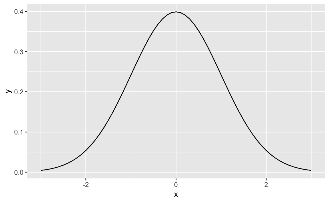
Figure 8-1 shows the smooth density function.
All the built-in probability distributions include a density function.
For a particular density, the function name is “d” prepended to the
density name. The density function for the Normal distribution is
dnorm, the density for the gamma distribution is dgamma, and so
forth.
If the first argument of the density function is a vector, then the function calculates the density at each point and returns the vector of densities.
The following code creates a 2 × 2 plot of four densities:
x<-seq(from=0,to=6,length.out=100)# Define the density domainsylim<-c(0,0.6)# Make a data.frame with densities of several distributionsdf<-rbind(data.frame(x=x,dist_name="Uniform",y=dunif(x,min=2,max=4)),data.frame(x=x,dist_name="Normal",y=dnorm(x,mean=3,sd=1)),data.frame(x=x,dist_name="Exponential",y=dexp(x,rate=1/2)),data.frame(x=x,dist_name="Gamma",y=dgamma(x,shape=2,rate=1)))# Make a line plot like before, but use facet_wrap to create the gridggplot(data=df,aes(x=x,y=y))+geom_line()+facet_wrap(~dist_name)# facet and wrap by the variable dist_name
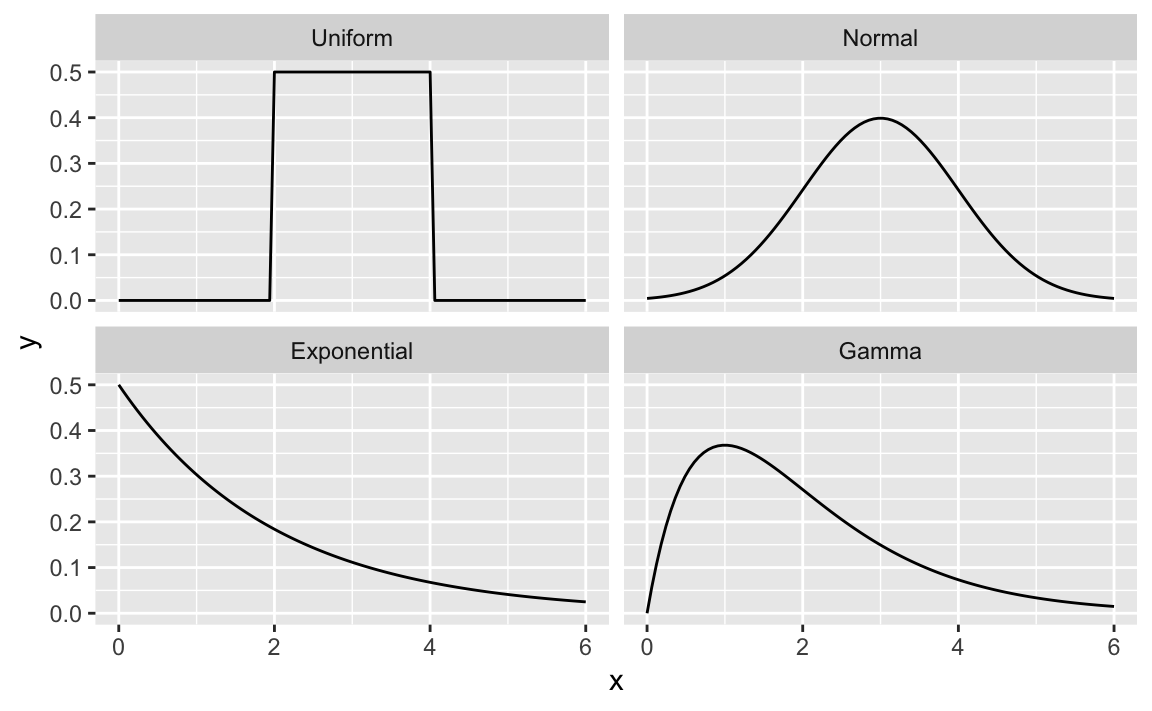
Figure 8-2 shows four density plots. However, a raw density plot is rarely useful or interesting by itself, and we often shade a region of interest.
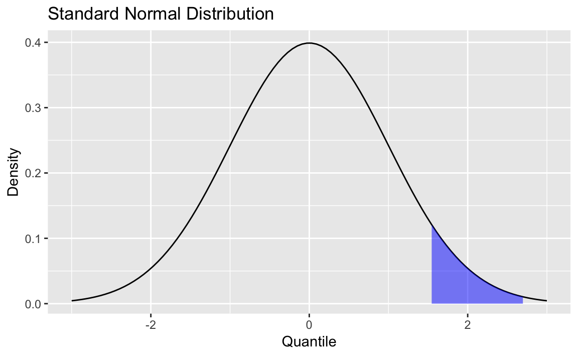
Figure 8-3 is a normal distribution with shading from the 75th percentile to the 95th percentile.
We create the plot by first plotting the density and then creating a
shaded region with the geom_ribbon function from ggplot2.
First, we create some data and draw the density curve shown in Figure 8-4
x<-seq(from=-3,to=3,length.out=100)df<-data.frame(x=x,y=dnorm(x,mean=0,sd=1))p<-ggplot(df,aes(x,y))+geom_line()+labs(title="Standard Normal Distribution",y="Density",x="Quantile")p
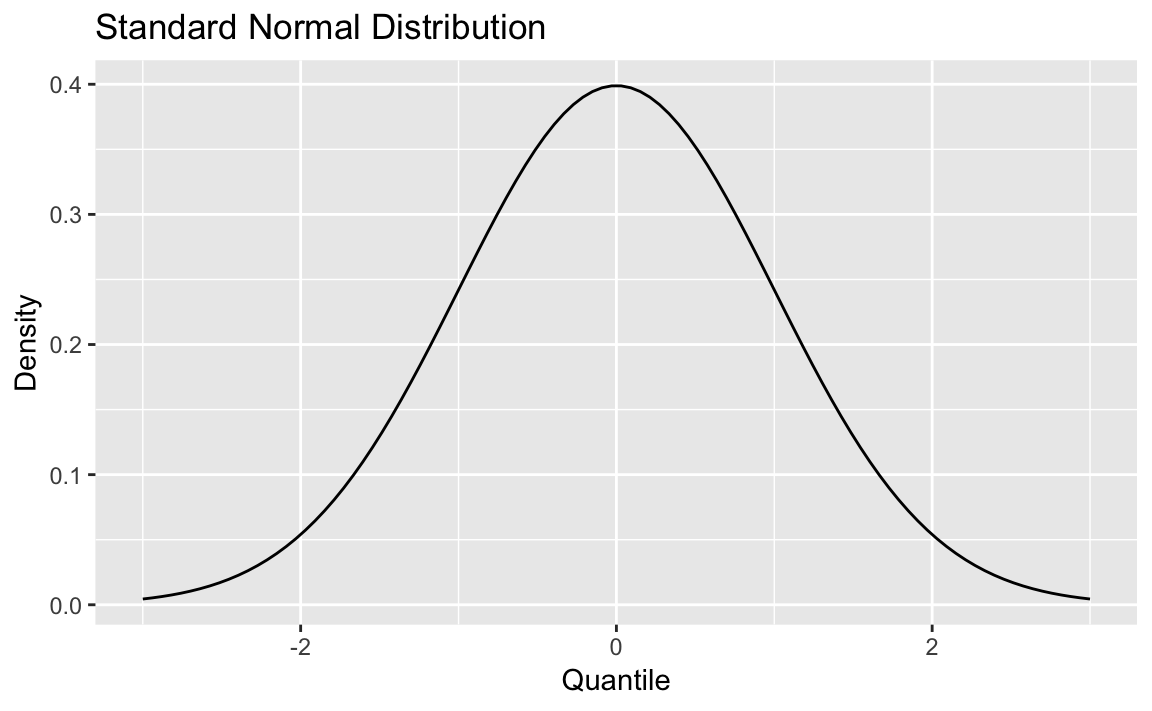
Next, we define the region of interest by calculating the x value for
the quantiles we’re interested in. Then finally we add a geom_ribbon
to add a subset of our original data as a colored region. The resulting
plot is shown here:
q75<-quantile(df$x,.75)q95<-quantile(df$x,.95)p+geom_ribbon(data=subset(df,x>q75&x<q95),aes(ymax=y),ymin=0,fill="blue",colour=NA,alpha=0.5)
Any significant application of R includes statistics or models or graphics. This chapter addresses the statistics. Some recipes simply describe how to calculate a statistic, such as relative frequency. Most recipes involve statistical tests or confidence intervals. The statistical tests let you choose between two competing hypotheses; that paradigm is described next. Confidence intervals reflect the likely range of a population parameter and are calculated based on your data sample.
Many of the statistical tests in this chapter use a time-tested paradigm of statistical inference. In the paradigm, we have one or two data samples. We also have two competing hypotheses, either of which could reasonably be true.
One hypothesis, called the null hypothesis, is that nothing happened: the mean was unchanged; the treatment had no effect; you got the expected answer; the model did not improve; and so forth.
The other hypothesis, called the alternative hypothesis, is that something happened: the mean rose; the treatment improved the patients’ health; you got an unexpected answer; the model fit better; and so forth.
We want to determine which hypothesis is more likely in light of the data:
To begin, we assume that the null hypothesis is true.
We calculate a test statistic. It could be something simple, such as the mean of the sample, or it could be quite complex. The critical requirement is that we must know the statistic’s distribution. We might know the distribution of the sample mean, for example, by invoking the Central Limit Theorem.
From the statistic and its distribution we can calculate a p-value, the probability of a test statistic value as extreme or more extreme than the one we observed, while assuming that the null hypothesis is true.
If the p-value is too small, we have strong evidence against the null hypothesis. This is called rejecting the null hypothesis.
If the p-value is not small then we have no such evidence. This is called failing to reject the null hypothesis.
There is one necessary decision here: When is a p-value “too small”?
In this book, we follow the common convention that we reject the null hypothesis when p < 0.05 and fail to reject it when p > 0.05. In statistical terminology, we chose a significance level of α = 0.05 to define the border between strong evidence and insufficient evidence against the null hypothesis.
But the real answer is, “it depends”. Your chosen significance level depends on your problem domain. The conventional limit of p < 0.05 works for many problems. In our work, the data are especially noisy and so we are often satisfied with p < 0.10. For someone working in high-risk areas, p < 0.01 or p < 0.001 might be necessary.
In the recipes, we mention which tests include a p-value so that you can compare the p-value against your chosen significance level of α. We worded the recipes to help you interpret the comparison. Here is the wording from “Testing Categorical Variables for Independence”, a test for the independence of two factors:
Conventionally, a p-value of less than 0.05 indicates that the variables are likely not independent whereas a p-value exceeding 0.05 fails to provide any such evidence.
This is a compact way of saying:
The null hypothesis is that the variables are independent.
The alternative hypothesis is that the variables are not independent.
For α = 0.05, if p < 0.05 then we reject the null hypothesis, giving strong evidence that the variables are not independent; if p > 0.05, we fail to reject the null hypothesis.
You are free to choose your own α, of course, in which case your decision to reject or fail to reject might be different.
Remember, the recipe states the informal interpretation of the test results, not the rigorous mathematical interpretation. We use colloquial language in the hope that it will guide you toward a practical understanding and application of the test. If the precise semantics of hypothesis testing is critical for your work, we urge you to consult the reference cited under See Also or one of the other fine textbooks on mathematical statistics.
Hypothesis testing is a well-understood mathematical procedure, but it can be frustrating. First, the semantics is tricky. The test does not reach a definite, useful conclusion. You might get strong evidence against the null hypothesis, but that’s all you’ll get. Second, it does not give you a number, only evidence.
If you want numbers then use confidence intervals, which bound the estimate of a population parameter at a given level of confidence. Recipes in this chapter can calculate confidence intervals for means, medians, and proportions of a population.
For example, “Forming a Confidence Interval for a Mean” calculates a 95% confidence interval for the population mean based on sample data. The interval is 97.16 < μ < 103.98, which means there is a 95% probability that the population’s mean, μ, is between 97.16 and 103.98.
Statistical terminology and conventions can vary. This book generally follows the conventions of Mathematical Statistics with Applications, 6th ed., by Wackerly et al. (Duxbury Press). We recommend this book also for learning more about the statistical tests described in this chapter.
You want a basic statistical summary of your data.
The summary function gives some useful statistics for vectors,
matrices, factors, and data frames:
summary(vec)#> Min. 1st Qu. Median Mean 3rd Qu. Max.#> 0.0 0.5 1.0 1.6 1.9 33.0
The Solution exhibits the summary of a vector. The 1st Qu. and
3rd Qu. are the first and third quartile, respectively. Having both
the median and mean is useful because you can quickly detect skew. The
Solution above, for example, shows a mean that is larger than the
median; this indicates a possible skew to the right, as one would expect
from a lognormal distribution.
The summary of a matrix works column by column. Here we see the summary
of a matrix, mat, with three columns named Samp1, Samp2, and
Samp3:
summary(mat)#> Samp1 Samp2 Samp3#> Min. : 1.0 Min. :-2.943 Min. : 0.04#> 1st Qu.: 25.8 1st Qu.:-0.774 1st Qu.: 0.39#> Median : 50.5 Median :-0.052 Median : 0.85#> Mean : 50.5 Mean :-0.067 Mean : 1.60#> 3rd Qu.: 75.2 3rd Qu.: 0.684 3rd Qu.: 2.12#> Max. :100.0 Max. : 2.150 Max. :13.18
The summary of a factor gives counts:
summary(fac)#> Maybe No Yes#> 38 32 30
The summary of a character vector is pretty useless, just the vector length:
summary(char)#> Length Class Mode#> 100 character character
The summary of a data frame incorporates all these features. It works column by column, giving an appropriate summary according to the column type. Numeric values receive a statistical summary and factors are counted (character strings are not summarized):
suburbs<-read_csv("./data/suburbs.txt")summary(suburbs)#> city county state#> Length:17 Length:17 Length:17#> Class :character Class :character Class :character#> Mode :character Mode :character Mode :character#>#>#>#> pop#> Min. : 5428#> 1st Qu.: 72616#> Median : 83048#> Mean : 249770#> 3rd Qu.: 102746#> Max. :2853114
The “summary” of a list is pretty funky: just the data type of each list
member. Here is a summary of a list of vectors:
summary(vec_list)#> Length Class Mode#> x 100 -none- numeric#> y 100 -none- numeric#> z 100 -none- character
To summarize the data inside a list of vectors, map summary to each
list element:
library(purrr)map(vec_list,summary)#> $x#> Min. 1st Qu. Median Mean 3rd Qu. Max.#> -2.572 -0.686 -0.084 -0.043 0.660 2.413#>#> $y#> Min. 1st Qu. Median Mean 3rd Qu. Max.#> -1.752 -0.589 0.045 0.079 0.769 2.293#>#> $z#> Length Class Mode#> 100 character character
Unfortunately, the summary function does not compute any measure of
variability, such as standard deviation or median absolute deviation.
This is a serious shortcoming, so we usually call sd or mad right
after calling summary.
See Recipes “Computing Basic Statistics” and .
You want to count the relative frequency of certain observations in your sample.
Identify the interesting observations by using a logical expression;
then use the mean function to calculate the fraction of observations
it identifies. For example, given a vector x, you can find the
relative frequency of positive values in this way:
mean(x>3)#> [1] 0.12
A logical expression, such as x > 3, produces a vector of logical
values (TRUE and FALSE), one for each element of x. The mean
function converts those values to 1s and 0s, respectively, and computes
the average. This gives the fraction of values that are TRUE—in other
words, the relative frequency of the interesting values. In the
Solution, for example, that’s the relative frequency of values greater
than 3.
The concept here is pretty simple. The tricky part is dreaming up a suitable logical expression. Here are some examples:
mean(lab == “NJ”)Fraction of lab values that are New Jersey
mean(after > before)Fraction of observations for which the effect increases
mean(abs(x-mean(x)) > 2*sd(x))Fraction of observations that exceed two standard deviations from the mean
mean(diff(ts) > 0)Fraction of observations in a time series that are larger than the previous observation
You want to tabulate one factor or to build a contingency table from multiple factors.
The table function produces counts of one factor:
table(f1)#> f1#> a b c d e#> 14 23 24 21 18
It can also produce contingency tables (cross-tabulations) from two or more factors:
table(f1,f2)#> f2#> f1 f g h#> a 6 4 4#> b 7 9 7#> c 4 11 9#> d 7 8 6#> e 5 10 3
table works for characters, too, not only factors:
t1<-sample(letters[9:11],100,replace=TRUE)table(t1)#> t1#> i j k#> 20 40 40
The table function counts the levels of one factor or characters, such
as these counts of initial and outcome (which are factors):
set.seed(42)initial<-factor(sample(c("Yes","No","Maybe"),100,replace=TRUE))outcome<-factor(sample(c("Pass","Fail"),100,replace=TRUE))table(initial)#> initial#> Maybe No Yes#> 39 31 30table(outcome)#> outcome#> Fail Pass#> 56 44
The greater power of table is in producing contingency tables, also
known as cross-tabulations. Each cell in a contingency table counts how
many times that row–column combination occurred:
table(initial,outcome)#> outcome#> initial Fail Pass#> Maybe 23 16#> No 20 11#> Yes 13 17
This table shows that the combination of initial = Yes and
outcome = Fail occurred 13 times, the combination of initial = Yes
and outcome = Pass occurred 17 times, and so forth.
The xtabs function can also produce a contingency table. It has a
formula interface, which some people prefer.
You have two categorical variables that are represented by factors. You want to test them for independence using the chi-squared test.
Use the table function to produce a contingency table from the two
factors. Then use the summary function to perform a chi-squared test
of the contingency table. In the example below we have two vectors of
factor values which we created in the prior recipe:
summary(table(initial,outcome))#> Number of cases in table: 100#> Number of factors: 2#> Test for independence of all factors:#> Chisq = 3, df = 2, p-value = 0.2
The output includes a p-value. Conventionally, a p-value of less than 0.05 indicates that the variables are likely not independent whereas a p-value exceeding 0.05 fails to provide any such evidence.
This example performs a chi-squared test on the contingency table of “Tabulating Factors and Creating Contingency Tables” and yields a p-value of 0.2225:
summary(table(initial,outcome))#> Number of cases in table: 100#> Number of factors: 2#> Test for independence of all factors:#> Chisq = 3, df = 2, p-value = 0.2
The large p-value indicates that the two factors, initial and
outcome, are probably independent. Practically speaking, we conclude
there is no connection between the variables. This makes sense as this
example data was created by simply drawing random data using the
sample function in the prior recipe.
The chisq.test function can also perform this test.
Given a fraction f, you want to know the corresponding quantile of your data. That is, you seek the observation x such that the fraction of observations below x is f.
Use the quantile function. The second argument is the fraction, f:
quantile(vec,0.95)#> 95%#> 1.43
For quartiles, simply omit the second argument altogether:
quantile(vec)#> 0% 25% 50% 75% 100%#> -2.0247 -0.5915 -0.0693 0.4618 2.7019
Suppose vec contains 1,000 observations between 0 and 1. The
quantile function can tell you which observation delimits the lower 5%
of the data:
vec<-runif(1000)quantile(vec,.05)#> 5%#> 0.0451
The quantile documentation refers to the second argument as a
“probability”, which is natural when we think of probability as meaning
relative frequency.
In true R style, the second argument can be a vector of probabilities;
in this case, quantile returns a vector of corresponding quantiles,
one for each probability:
quantile(vec,c(.05,.95))#> 5% 95%#> 0.0451 0.9363
That is a handy way to identify the middle 90% (in this case) of the observations.
If you omit the probabilities altogether then R assumes you want the probabilities 0, 0.25, 0.50, 0.75, and 1.0—in other words, the quartiles:
quantile(vec)#> 0% 25% 50% 75% 100%#> 0.000405 0.235529 0.479543 0.737619 0.999379
Amazingly, the quantile function implements nine (yes, nine) different
algorithms for computing quantiles. Study the help page before assuming
that the default algorithm is the best one for you.
Given an observation x from your data, you want to know its corresponding quantile. That is, you want to know what fraction of the data is less than x.
Assuming your data is in a vector vec, compare the data against the
observation and then use mean to compute the relative frequency of
values less than x; say, 1.6 as per this example.
mean(vec<1.6)#> [1] 0.948
The expression vec < x compares every element of vec against x and
returns a vector of logical values, where the n_th logical value is
TRUE if vec[n] < x. The mean function converts those logical
values to 0 and 1: 0 for FALSE and 1 for TRUE. The average of all
those 1s and 0s is the fraction of vec that is less than _x, or the
inverse quantile of x.
This is an application of the general approach described in “Calculating Relative Frequencies”.
You have a dataset, and you want to calculate the corresponding z-scores for all data elements. (This is sometimes called normalizing the data.)
Use the scale function:
scale(x)#> [,1]#> [1,] 0.8701#> [2,] -0.7133#> [3,] -1.0503#> [4,] 0.5790#> [5,] -0.6324#> [6,] 0.0991#> [7,] 2.1495#> [8,] 0.2481#> [9,] -0.8155#> [10,] -0.7341#> attr(,"scaled:center")#> [1] 2.42#> attr(,"scaled:scale")#> [1] 2.11
This works for vectors, matrices, and data frames. In the case of a
vector, scale returns the vector of normalized values. In the case of
matrices and data frames, scale normalizes each column independently
and returns columns of normalized values in a matrix.
You might also want to normalize a single value y relative to a dataset x. That can be done by using vectorized operations as follows:
(y-mean(x))/sd(x)#> [1] -0.633
You have a sample from a population. Given this sample, you want to know if the mean of the population could reasonably be a particular value m.
Apply the t.test function to the sample x with the argument mu=m:
t.test(x,mu=m)
The output includes a p-value. Conventionally, if p < 0.05 then the population mean is unlikely to be m whereas p > 0.05 provides no such evidence.
If your sample size n is small, then the underlying population must be normally distributed in order to derive meaningful results from the t test. A good rule of thumb is that “small” means n < 30.
The t test is a workhorse of statistics, and this is one of its basic
uses: making inferences about a population mean from a sample. The
following example simulates sampling from a normal population with mean
μ = 100. It uses the t test to ask if the population mean could be
95, and t.test reports a p-value of 0.005055:
x<-rnorm(75,mean=100,sd=15)t.test(x,mu=95)#>#> One Sample t-test#>#> data: x#> t = 3, df = 70, p-value = 0.005#> alternative hypothesis: true mean is not equal to 95#> 95 percent confidence interval:#> 96.5 103.0#> sample estimates:#> mean of x#> 99.7
The p-value is small and so it’s unlikely (based on the sample data) that 95 could be the mean of the population.
Informally, we could interpret the low p-value as follows. If the population mean were really 95, then the probability of observing our test statistic (t = 2.8898 or something more extreme) would be only 0.005055 That is very improbable, yet that is the value we observed. Hence we conclude that the null hypothesis is wrong; therefore, the sample data does not support the claim that the population mean is 95.
In sharp contrast, testing for a mean of 100 gives a p-value of 0.8606:
t.test(x,mu=100)#>#> One Sample t-test#>#> data: x#> t = -0.2, df = 70, p-value = 0.9#> alternative hypothesis: true mean is not equal to 100#> 95 percent confidence interval:#> 96.5 103.0#> sample estimates:#> mean of x#> 99.7
The large p-value indicates that the sample is consistent with assuming a population mean μ of 100. In statistical terms, the data does not provide evidence against the true mean being 100.
A common case is testing for a mean of zero. If you omit the mu
argument, it defaults to zero.
You have a sample from a population. Given that sample, you want to determine a confidence interval for the population’s mean.
Apply the t.test function to your sample x:
t.test(x)
The output includes a confidence interval at the 95% confidence level.
To see intervals at other levels, use the conf.level argument.
As in “Testing the Mean of a Sample (t Test)”, if your sample size n is small then the underlying population must be normally distributed for there to be a meaningful confidence interval. Again, a good rule of thumb is that “small” means n < 30.
Applying the t.test function to a vector yields a lot of output.
Buried in the output is a confidence interval:
t.test(x)#>#> One Sample t-test#>#> data: x#> t = 50, df = 50, p-value <2e-16#> alternative hypothesis: true mean is not equal to 0#> 95 percent confidence interval:#> 94.2 101.5#> sample estimates:#> mean of x#> 97.9
In this example, the confidence interval is approximately 94.16 < μ < 101.55, which is sometimes written simply as (94.16, 101.55).
We can raise the confidence level to 99% by setting conf.level=0.99:
t.test(x,conf.level=0.99)#>#> One Sample t-test#>#> data: x#> t = 50, df = 50, p-value <2e-16#> alternative hypothesis: true mean is not equal to 0#> 99 percent confidence interval:#> 92.9 102.8#> sample estimates:#> mean of x#> 97.9
That change widens the confidence interval to 92.93 < μ < 102.78
You have a data sample, and you want to know the confidence interval for the median.
Use the wilcox.test function, setting conf.int=TRUE:
wilcox.test(x,conf.int=TRUE)
The output will contain a confidence interval for the median.
The procedure for calculating the confidence interval of a mean is well-defined and widely known. The same is not true for the median, unfortunately. There are several procedures for calculating the median’s confidence interval. None of them is “the” procedure, but the Wilcoxon signed rank test is pretty standard.
The wilcox.test function implements that procedure. Buried in the
output is the 95% confidence interval, which is approximately (-0.102,
0.646) in this case:
wilcox.test(x,conf.int=TRUE)#>#> Wilcoxon signed rank test#>#> data: x#> V = 200, p-value = 0.1#> alternative hypothesis: true location is not equal to 0#> 95 percent confidence interval:#> -0.102 0.646#> sample estimates:#> (pseudo)median#> 0.311
You can change the confidence level by setting conf.level, such as
conf.level=0.99 or other such values.
The output also includes something called the pseudomedian, which is defined on the help page. Don’t assume it equals the median; they are different:
median(x)#> [1] 0.314
You have a sample of values from a population consisting of successes and failures. You believe the true proportion of successes is p, and you want to test that hypothesis using the sample data.
Use the prop.test function. Suppose the sample size is n and the
sample contains x successes:
prop.test(x,n,p)
The output includes a p-value. Conventionally, a p-value of less than 0.05 indicates that the true proportion is unlikely to be p whereas a p-value exceeding 0.05 fails to provide such evidence.
Suppose you encounter some loudmouthed fan of the Chicago Cubs early in the baseball season. The Cubs have played 20 games and won 11 of them, or 55% of their games. Based on that evidence, the fan is “very confident” that the Cubs will win more than half of their games this year. Should he be that confident?
The prop.test function can evaluate the fan’s logic. Here, the number
of observations is n = 20, the number of successes is x = 11, and
p is the true probability of winning a game. We want to know whether
it is reasonable to conclude, based on the data, that p > 0.5.
Normally, prop.test would check for p ≠ 0.05 but we can check for
p > 0.5 instead by setting alternative="greater":
prop.test(11,20,0.5,alternative="greater")#>#> 1-sample proportions test with continuity correction#>#> data: 11 out of 20, null probability 0.5#> X-squared = 0.05, df = 1, p-value = 0.4#> alternative hypothesis: true p is greater than 0.5#> 95 percent confidence interval:#> 0.35 1.00#> sample estimates:#> p#> 0.55
The prop.test output shows a large p-value, 0.4115, so we cannot
reject the null hypothesis; that is, we cannot reasonably conclude that
p is greater than 1/2. The Cubs fan is being overly confident based on
too little data. No surprise there.
You have a sample of values from a population consisting of successes and failures. Based on the sample data, you want to form a confidence interval for the population’s proportion of successes.
Use the prop.test function. Suppose the sample size is n and the
sample contains x successes:
prop.test(x,n)
The function output includes the confidence interval for p.
We subscribe to a stock market newsletter that is well written, but includes a section purporting to identify stocks that are likely to rise. It does this by looking for a certain pattern in the stock price. It recently reported, for example, that a certain stock was following the pattern. It also reported that the stock rose six times after the last nine times that pattern occurred. The writers concluded that the probability of the stock rising again was therefore 6/9 or 66.7%.
Using prop.test, we can obtain the confidence interval for the true
proportion of times the stock rises after the pattern. Here, the number
of observations is n = 9 and the number of successes is x = 6. The
output shows a confidence interval of (0.309, 0.910) at the 95%
confidence level:
prop.test(6,9)#> Warning in prop.test(6, 9): Chi-squared approximation may be incorrect#>#> 1-sample proportions test with continuity correction#>#> data: 6 out of 9, null probability 0.5#> X-squared = 0.4, df = 1, p-value = 0.5#> alternative hypothesis: true p is not equal to 0.5#> 95 percent confidence interval:#> 0.309 0.910#> sample estimates:#> p#> 0.667
The writers are pretty foolish to say the probability of rising is 66.7%. They could be leading their readers into a very bad bet.
By default, prop.test calculates a confidence interval at the 95%
confidence level. Use the conf.level argument for other confidence
levels:
prop.test(x,n,p,conf.level=0.99)# 99% confidence level
You want a statistical test to determine whether your data sample is from a normally distributed population.
Use the shapiro.test function:
shapiro.test(x)
The output includes a p-value. Conventionally, p < 0.05 indicates that the population is likely not normally distributed whereas p > 0.05 provides no such evidence.
This example reports a p-value of .7765 for x:
shapiro.test(x)#>#> Shapiro-Wilk normality test#>#> data: x#> W = 1, p-value = 0.05
The large p-value suggests the underlying population could be normally distributed. The next example reports a very small p-value for y, so it is unlikely that this sample came from a normal population:
shapiro.test(y)#>#> Shapiro-Wilk normality test#>#> data: y#> W = 0.7, p-value = 9e-12
We have highlighted the Shapiro–Wilk test because it is a standard R
function. You can also install the package nortest, which is dedicated
entirely to tests for normality. This package includes:
Anderson–Darling test (ad.test)
Cramer–von Mises test (cvm.test)
Lilliefors test (lillie.test)
Pearson chi-squared test for the composite hypothesis of normality
(pearson.test)
Shapiro–Francia test (sf.test)
The problem with all these tests is their null hypothesis: they all assume that the population is normally distributed until proven otherwise. As a result, the population must be decidedly nonnormal before the test reports a small p-value and you can reject that null hypothesis. That makes the tests quite conservative, tending to err on the side of normality.
Instead of depending solely upon a statistical test, we suggest also using histograms (“Creating a Histogram”) and quantile-quantile plots (“Creating a Normal Quantile-Quantile (Q-Q) Plot”) to evaluate the normality of any data. Are the tails too fat? Is the peak to peaked? Your judgment is likely better than a single statistical test.
See “Installing Packages from CRAN” for how to install the nortest package.
Your data is a sequence of binary values: yes–no, 0–1, true–false, or other two-valued data. You want to know: Is the sequence random?
The tseries package contains the runs.test function, which checks a
sequence for randomness. The sequence should be a factor with two
levels:
library(tseries)runs.test(as.factor(s))
The runs.test function reports a p-value. Conventionally, a
p-value of less than 0.05 indicates that the sequence is likely not
random whereas a p-value exceeding 0.05 provides no such evidence.
A run is a subsequence composed of identical values, such as all 1s or all 0s. A random sequence should be properly jumbled up, without too many runs. Similarly, it shouldn’t contain too few runs, either. A sequence of perfectly alternating values (0, 1, 0, 1, 0, 1, …) contains no runs, but would you say that it’s random?
The runs.test function checks the number of runs in your sequence. If
there are too many or too few, it reports a small p-value.
This first example generates a random sequence of 0s and 1s and then
tests the sequence for runs. Not surprisingly, runs.test reports a
large p-value, indicating the sequence is likely random:
s<-sample(c(0,1),100,replace=T)runs.test(as.factor(s))#>#> Runs Test#>#> data: as.factor(s)#> Standard Normal = 0.1, p-value = 0.9#> alternative hypothesis: two.sided
This next sequence, however, consists of three runs and so the reported p-value is quite low:
s<-c(0,0,0,0,1,1,1,1,0,0,0,0)runs.test(as.factor(s))#>#> Runs Test#>#> data: as.factor(s)#> Standard Normal = -2, p-value = 0.02#> alternative hypothesis: two.sided
You have one sample each from two populations. You want to know if the two populations could have the same mean.
Perform a t test by calling the t.test function:
t.test(x,y)
By default, t.test assumes that your data are not paired. If the
observations are paired (i.e., if each xi is paired with one
yi), then specify paired=TRUE:
t.test(x,y,paired=TRUE)
In either case, t.test will compute a p-value. Conventionally, if
p < 0.05 then the means are likely different whereas p > 0.05
provides no such evidence:
If either sample size is small, then the populations must be normally distributed. Here, “small” means fewer than 20 data points.
If the two populations have the same variance, specify
var.equal=TRUE to obtain a less conservative test.
We often use the t test to get a quick sense of the difference between two population means. It requires that the samples be large enough (both samples have 20 or more observations) or that the underlying populations be normally distributed. We don’t take the “normally distributed” part too literally. Being bell-shaped and reasonably symetrical should be good enough.
A key distinction here is whether or not your data contains paired observations, since the results may differ in the two cases. Suppose we want to know if coffee in the morning improves scores on SAT tests. We could run the experiment two ways:
Randomly select one group of people. Give them the SAT test twice, once with morning coffee and once without morning coffee. For each person, we will have two SAT scores. These are paired observations.
Randomly select two groups of people. One group has a cup of morning coffee and takes the SAT test. The other group just takes the test. We have a score for each person, but the scores are not paired in any way.
Statistically, these experiments are quite different. In experiment 1, there are two observations for each person (caffeinated and decaf) and they are not statistically independent. In experiment 2, the data are independent.
If you have paired observations (experiment 1) and erroneously analyze them as unpaired observations (experiment 2), then you could get this result with a p-value of 0.9867:
load("./data/sat.rdata")t.test(x,y)#>#> Welch Two Sample t-test#>#> data: x and y#> t = -1, df = 200, p-value = 0.3#> alternative hypothesis: true difference in means is not equal to 0#> 95 percent confidence interval:#> -46.4 16.2#> sample estimates:#> mean of x mean of y#> 1054 1069
The large p-value forces you to conclude there is no difference between the groups. Contrast that result with the one that follows from analyzing the same data but correctly identifying it as paired:
t.test(x,y,paired=TRUE)#>#> Paired t-test#>#> data: x and y#> t = -20, df = 100, p-value <2e-16#> alternative hypothesis: true difference in means is not equal to 0#> 95 percent confidence interval:#> -16.8 -13.5#> sample estimates:#> mean of the differences#> -15.1
The p-value plummets to 2.2e-16, and we reach the exactly opposite conclusion.
If the populations are not normally distributed (bell-shaped) and either sample is small, consider using the Wilcoxon–Mann–Whitney test described in “Comparing the Locations of Two Samples Nonparametrically”.
You have samples from two populations. You don’t know the distribution of the populations, but you know they have similar shapes. You want to know: Is one population shifted to the left or right compared with the other?
You can use a nonparametric test, the Wilcoxon–Mann–Whitney test, which
is implemented by the wilcox.test function. For paired observations
(every xi is paired with yi), set paired=TRUE:
wilcox.test(x,y,paired=TRUE)
For unpaired observations, let paired default to FALSE:
wilcox.test(x,y)
The test output includes a p-value. Conventionally, a p-value of less than 0.05 indicates that the second population is likely shifted left or right with respect to the first population whereas a p-value exceeding 0.05 provides no such evidence.
When we stop making assumptions regarding the distributions of populations, we enter the world of nonparametric statistics. The Wilcoxon–Mann–Whitney test is nonparametric and so can be applied to more datasets than the t test, which requires that the data be normally distributed (for small samples). This test’s only assumption is that the two populations have the same shape.
In this recipe, we are asking: Is the second population shifted left or right with respect to the first? This is similar to asking whether the average of the second population is smaller or larger than the first. However, the Wilcoxon–Mann–Whitney test answers a different question: it tells us whether the central locations of the two populations are significantly different or, equivalently, whether their relative frequencies are different.
Suppose we randomly select a group of employees and ask each one to complete the same task under two different circumstances: under favorable conditions and under unfavorable conditions, such as a noisy environment. We measure their completion times under both conditions, so we have two measurements for each employee. We want to know if the two times are significantly different, but we can’t assume they are normally distributed.
The data are paired, so we must set paired=TRUE:
load(file="./data/workers.rdata")wilcox.test(fav,unfav,paired=TRUE)#>#> Wilcoxon signed rank test#>#> data: fav and unfav#> V = 10, p-value = 1e-04#> alternative hypothesis: true location shift is not equal to 0
The p-value is essentially zero. Statistically speaking, we reject the assumption that the completion times were equal. Practically speaking, it’s reasonable to conclude that the times were different.
In this example, setting paired=TRUE is critical. Treating the data as
unpaired would be wrong because the observations are not independent;
and this, in turn, would produce bogus results. Running the example with
paired=FALSE produces a p-value of 0.1022, which leads to the wrong
conclusion.
See “Comparing the Means of Two Samples” for the parametric test.
You calculated the correlation between two variables, but you don’t know if the correlation is statistically significant.
The cor.test function can calculate both the p-value and the
confidence interval of the correlation. If the variables came from
normally distributed populations then use the default measure of
correlation, which is the Pearson method:
cor.test(x,y)
For nonnormal populations, use the Spearman method instead:
cor.test(x,y,method="spearman")
The function returns several values, including the p-value from the test of significance. Conventionally, p < 0.05 indicates that the correlation is likely significant whereas p > 0.05 indicates it is not.
In my experience, people often fail to check a correlation for
significance. In fact, many people are unaware that a correlation can be
insignificant. They jam their data into a computer, calculate the
correlation, and blindly believe the result. However, they should ask
themselves: Was there enough data? Is the magnitude of the correlation
large enough? Fortunately, the cor.test function answers those
questions.
Suppose we have two vectors, x and y, with values from normal populations. We might be very pleased that their correlation is greater than 0.75:
cor(x,y)#> [1] 0.751
But that is naïve. If we run cor.test, it reports a relatively large
p-value of 0.085:
cor.test(x,y)#>#> Pearson's product-moment correlation#>#> data: x and y#> t = 2, df = 4, p-value = 0.09#> alternative hypothesis: true correlation is not equal to 0#> 95 percent confidence interval:#> -0.155 0.971#> sample estimates:#> cor#> 0.751
The p-value is above the conventional threshold of 0.05, so we conclude that the correlation is unlikely to be significant.
You can also check the correlation by using the confidence interval. In this example, the confidence interval is (−0.155, 0.970). The interval contains zero and so it is possible that the correlation is zero, in which case there would be no correlation. Again, you could not be confident that the reported correlation is significant.
The cor.test output also includes the point estimate reported by cor
(at the bottom, labeled “sample estimates”), saving you the additional
step of running cor.
By default, cor.test calculates the Pearson correlation, which assumes
that the underlying populations are normally distributed. The Spearman
method makes no such assumption because it is nonparametric. Use
method="Spearman" when working with nonnormal data.
See “Computing Basic Statistics” for calculating simple correlations.
You have samples from two or more groups. The group’s elements are binary-valued: either success or failure. You want to know if the groups have equal proportions of successes.
Use the prop.test function with two vector arguments:
#> #> 2-sample test for equality of proportions with continuity #> correction #> #> data: ns out of nt #> X-squared = 5, df = 1, p-value = 0.03 #> alternative hypothesis: two.sided #> 95 percent confidence interval: #> -0.3058 -0.0142 #> sample estimates: #> prop 1 prop 2 #> 0.48 0.64
ns<-c(48,64)nt<-c(100,100)prop.test(ns,nt)
These are parallel vectors. The first vector, ns, gives the number of
successes in each group. The second vector, nt, gives the size of the
corresponding group (often called the number of trials).
The output includes a p-value. Conventionally, a p-value of less than 0.05 indicates that it is likely the groups’ proportions are different whereas a p-value exceeding 0.05 provides no such evidence.
In “Testing a Sample Proportion” we tested a proportion based on one sample. Here, we have samples from several groups and want to compare the proportions in the underlying groups.
One of the authors recently taught statistics to 38 students and awarded a grade of A to 14 of them. A colleague taught the same class to 40 students and awarded an A to only 10. We wanted to know: Is the author fostering grade inflation by awarding significantly more A grades than the other teacher did?
We used prop.test. “Success” means awarding an A, so the vector of
successes contains two elements: the number awarded by me and the number
awarded by my colleague:
successes<-c(14,10)
The number of trials is the number of students in the corresponding class:
trials<-c(38,40)
The prop.test output yields a p-value of 0.3749:
prop.test(successes,trials)#>#> 2-sample test for equality of proportions with continuity#> correction#>#> data: successes out of trials#> X-squared = 0.8, df = 1, p-value = 0.4#> alternative hypothesis: two.sided#> 95 percent confidence interval:#> -0.111 0.348#> sample estimates:#> prop 1 prop 2#> 0.368 0.250
The relatively large p-value means that we cannot reject the null hypothesis: the evidence does not suggest any difference between the teachers’ grading.
You have several samples, and you want to perform a pairwise comparison between the sample means. That is, you want to compare the mean of every sample against the mean of every other sample.
Place all data into one vector and create a parallel factor to identify
the groups. Use pairwise.t.test to perform the pairwise comparison of
means:
pairwise.t.test(x,f)# x is the data, f is the grouping factor
The output contains a table of p-values, one for each pair of groups. Conventionally, if p < 0.05 then the two groups likely have different means whereas p > 0.05 provides no such evidence.
This is more complicated than “Comparing the Means of Two Samples”, where we compared the means of two samples. Here we have several samples and want to compare the mean of every sample against the mean of every other sample.
Statistically speaking, pairwise comparisons are tricky. It is not the
same as simply performing a t test on every possible pair. The
p-values must be adjusted, for otherwise you will get an overly
optimistic result. The help pages for pairwise.t.test and p.adjust
describe the adjustment algorithms available in R. Anyone doing serious
pairwise comparisons is urged to review the help pages and consult a
good textbook on the subject.
Suppose we are using a larger sample of the data from
“Combining Multiple Vectors into One Vector and a Factor”, where we combined data for freshmen, sophomores, and juniors
into a data frame called comb. The data frame has two columns: the
data in a column called values, and the grouping factor in a column
called ind. We can use pairwise.t.test to perform pairwise
comparisons between the groups:
pairwise.t.test(comb$values,comb$ind)#>#> Pairwise comparisons using t tests with pooled SD#>#> data: comb$values and comb$ind#>#> fresh soph#> soph 0.001 -#> jrs 3e-04 0.592#>#> P value adjustment method: holm
Notice the table of p-values. The comparisons of juniors versus freshmen and of sophomores versus freshmen produced small p-values: 0.0011 and 0.0003, respectively. We can conclude there are significant differences between those groups. However, the comparison of sophomores versus juniors produced a (relatively) large p-value of 0.5922, so they are not significantly different.
You have two samples, and you are wondering: Did they come from the same distribution?
The Kolmogorov–Smirnov test compares two samples and tests them for
being drawn from the same distribution. The ks.test function
implements that test:
ks.test(x,y)
The output includes a p-value. Conventionally, a p-value of less than 0.05 indicates that the two samples (x and y) were drawn from different distributions whereas a p-value exceeding 0.05 provides no such evidence.
The Kolmogorov–Smirnov test is wonderful for two reasons. First, it is a nonparametric test and so you needn’t make any assumptions regarding the underlying distributions: it works for all distributions. Second, it checks the location, dispersion, and shape of the populations, based on the samples. If these characteristics disagree then the test will detect that, allowing us to conclude that the underlying distributions are different.
Suppose we suspect that the vectors x and y come from differing
distributions. Here, ks.test reports a p-value of 0.03663:
#> #> Two-sample Kolmogorov-Smirnov test #> #> data: x and y #> D = 0.2, p-value = 0.04 #> alternative hypothesis: two-sided
ks.test(x,y)#>#> Two-sample Kolmogorov-Smirnov test#>#> data: x and y#> D = 0.2, p-value = 0.04#> alternative hypothesis: two-sided
From the small p-value we can conclude that the samples are from different distributions. However, when we test x against another sample, z, the p-value is much larger (0.5806); this suggests that x and z could have the same underlying distribution:
z<-rnorm(100,mean=4,sd=6)ks.test(x,z)#>#> Two-sample Kolmogorov-Smirnov test#>#> data: x and z#> D = 0.1, p-value = 0.6#> alternative hypothesis: two-sided
Graphics is a great strength of R. The graphics package is part of the
standard distribution and contains many useful functions for creating a
variety of graphic displays. The base functionality has been expanded
and made easier with ggplot2, part of the tidyverse of packages. In
this chapter we will focus on examples using ggplot2, and we will
occasionally suggest other packages. In this chapter’s See Also sections
we mention functions in other packages that do the same job in a
different way. We suggest that you explore those alternatives if you are
dissatisfied with what’s offered by ggplot2 or base graphics.
Graphics is a vast subject, and we can only scratch the surface here.
Winston Chang’s R Graphics Cookbook, 2nd Edition is part of the
O’Reilly Cookbook series and walks through many useful recipes with a
focus on ggplot2. If you want to delve deeper, we recommend R
Graphics by Paul Murrell (Chapman & Hall, 2006). That book discusses
the paradigms behind R graphics, explains how to use the graphics
functions, and contains numerous examples—including the code to recreate
them. Some of the examples are pretty amazing.
The graphs in this chapter are mostly plain and unadorned. We did that
intentionally. When you call the ggplot function, as in:
library(tidyverse)
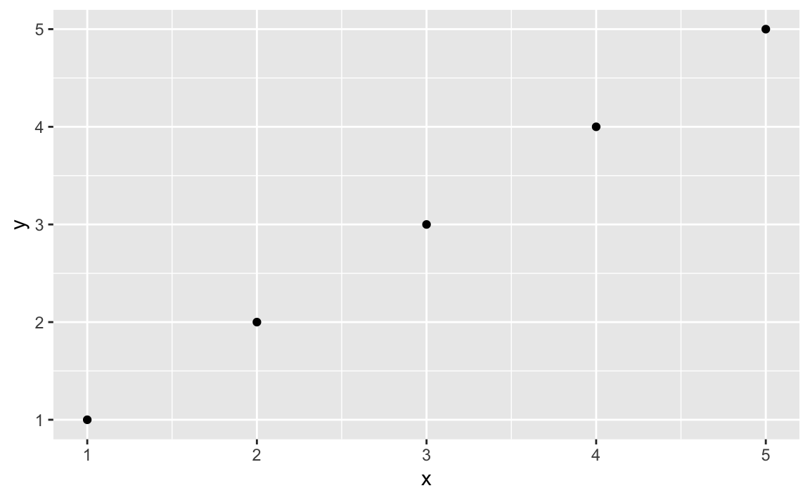
df<-data.frame(x=1:5,y=1:5)ggplot(df,aes(x,y))+geom_point()
you get a plain, graphical representation of x and y as shown in
Figure 10-1. You could adorn the graph with colors, a
title, labels, a legend, text, and so forth, but then the call to
ggplot becomes more and more crowded, obscuring the basic intention.
ggplot(df,aes(x,y))+geom_point()+labs(title="Simple Plot Example",subtitle="with a subtitle",x="x values",y="y values")+theme(panel.background=element_rect(fill="white",colour="grey50"))
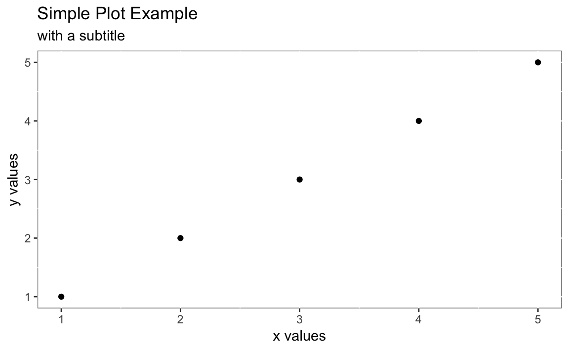
The resulting plot is shown in Figure 10-2. We want to keep the recipes clean, so we emphasize the basic plot and then show later (as in “Adding a Title and Labels”) how to add adornments.
ggplot2 basicsWhile the package is called ggplot2 the primary plotting function in
the package is called ggplot. It is important to understand the basic
pieces of a ggplot2 graph. In the examples above you can see that we
pass data into ggplot then define how the graph is created by stacking
together small phrases that describe some aspect of the plot. This
stacking together of phrases is part of the “grammar of graphics” ethos
(that’s where the gg comes from). To learn more, you can read “The
Layered Grammar of Graphics” written by ggplot2 author, Hadley Wickham
(http://vita.had.co.nz/papers/layered-grammar.pdf). The “grammar of
graphics,” concept originating with Leland Wilkinson who articulated the
idea of building graphics up from a set of primitives (i.e. verbs and
nouns). With ggplot, the underlying data need not be fundamentally
reshaped for each type of graphical representation. In general, the data
stays the same and the user then changes syntax slightly to illustrate
the data differently. This is significantly more consistent than base
graphics which often require reshaping the data in order to change the
way the data is visualized.
As we talk about ggplot graphics it’s worth defining the things that
make up a ggplot graph:
geometric object functionsThese are geometric objects that describe the type of graph being
created. These start with geom_ and examples include geom_line,
geom_boxplot, and geom_point along with dozens more.
aestheticsThe aesthetics, or aesthetic mappings, communicate to ggplot which
fields in the source data get mapped to which visual elements in the
graphic. This is the aes() line in a ggplot call.
statsStats are statistical transformations that are done before displaying
the data. Not all graphs will have stats, but a few common stats are
stat_ecdf (the empirical cumulative distribution function) and
stat_identity which tells ggplot to pass the data without doing
any stats at all.
facet functionsFacets are subplots where each small plot represents a subgroup of the
data. The faceting functions include facet_wrap and facet_grid.
themesThemes are the visual elements of the plot that are not tied to data. These might include titles, margins, table of contents locations, or font choices.
layerA layer is a combination of data, aesthetics, a geometric object, a
stat, and other options to produce a visual layer in the ggplot
graphic.
One of the first confusions new users to ggplot often face is that
they are inclined to reshape their data to be “wide” before plotting it.
Wide here meaning every variable they are plotting is its own column in
the underlying data frame.
ggplot works most easily with “long” data where additional variables
are added as rows in the data frame rather than columns. The great side
effect of adding additional measurements as rows is that any properly
constructed ggplot graphs will automatically update to reflect the new
data without changing the ggplot code. If each additional variable was
added as a column, then the plotting code would have to be changed to
introduce additional variables. This idea of “long” vs. “wide” data will
become more obvious in the examples in the rest of this chapter.
R is highly programmable, and many people have extended its graphics
machinery with additional features. Quite often, packages include
specialized functions for plotting their results and objects. The zoo
package, for example, implements a time series object. If you create a
zoo object z and call plot(z), then the zoo package does the
plotting; it creates a graphic that is customized for displaying a time
series. Zoo uses base graphics so the resulting graph will not be a
ggplot graphic.
There are even entire packages devoted to extending R with new graphics
paradigms. The lattice package is an alternative to base graphics that
predates ggplot2. It uses a powerful graphics paradigm that enables
you to create informative graphics more easily. It was implemented by
Deepayan Sarkar, who also wrote Lattice: Multivariate Data
Visualization with R (Springer, 2008), which explains the package and
how to use it. The lattice package is also described in
R in a Nutshell (O’Reilly).
There are two chapters in Hadley Wickham’s excellent book R for Data
Science which deal with graphics. The first, “Exploratory Data
Analysis” focuses on exploring data with ggplot2 while “Graphics for
Communication” explores communicating to others with graphics. R for
Data Science is availiable in a printed version from O’Reilly Media or
online at http://r4ds.had.co.nz/graphics-for-communication.html.
You have paired observations: (x1, y1), (x2, y2), …, (xn, yn). You want to create a scatter plot of the pairs.
We can plot the data by calling ggplot, passing in the data frame, and
invoking a geometric point function:
ggplot(df,aes(x,y))+geom_point()
In this example, the data frame is called df and the x and y data
are in fields named x and y which we pass to the aesthetic in the
call aes(x, y).
A scatter plot is a common first attack on a new dataset. It’s a quick way to see the relationship, if any, between x and y.
Plotting with ggplot requires telling ggplot what data frame to use,
then what type of graph to create, and which aesthetic mapping (aes) to
use . The aes in this case defines which field from df goes into
which axis on the plot. Then the command geom_point communicates that
you want a point graph, as opposed to a line or other type of graphic.
We can use the built in mtcars dataset to illustrate plotting
horsepower hp on the x axis and fuel economy mpg on the y:
ggplot(mtcars,aes(hp,mpg))+geom_point()
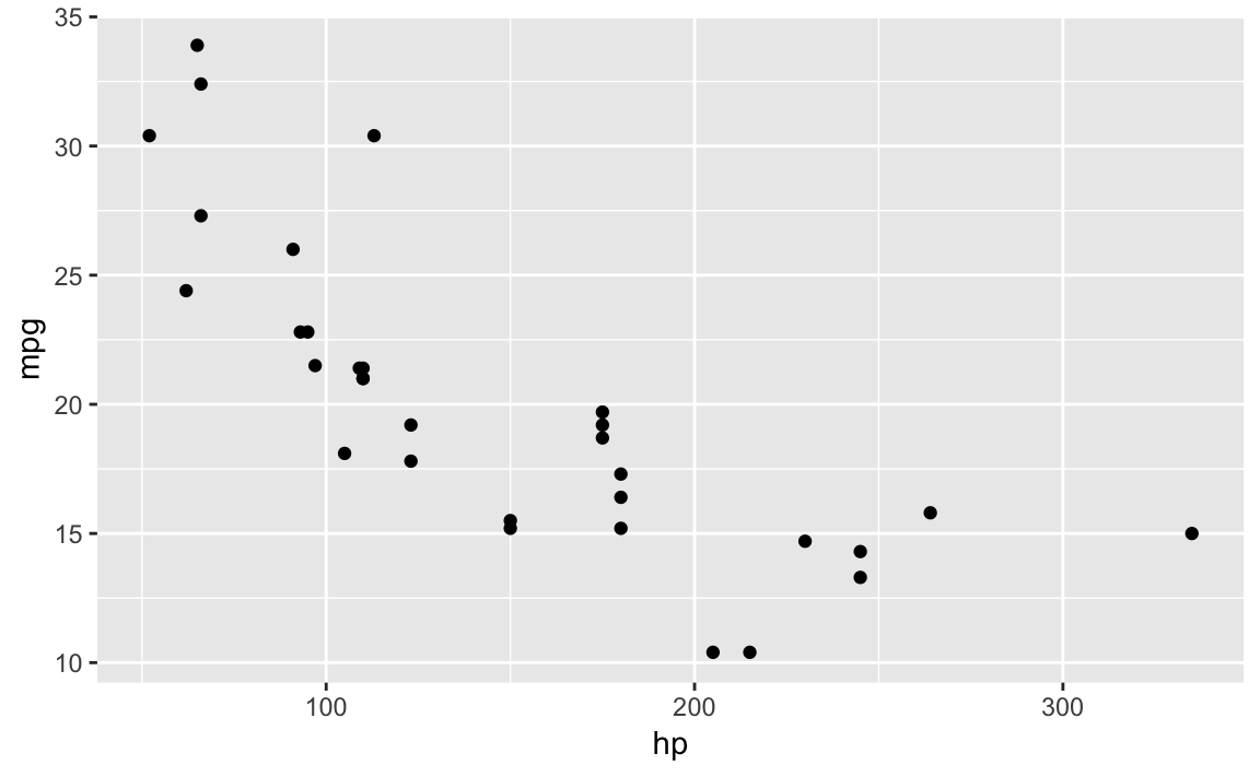
The resulting plot is shown in Figure 10-3.
See “Adding a Title and Labels” for adding a title and labels; see Recipes and for adding a grid and a legend (respectively). See “Plotting All Variables Against All Other Variables” for plotting multiple variables.
You want to add a title to your plot or add labels for the axes.
With ggplot we add a labs element which controls the labels for the
title and axies.
When calling labs in ggplot:
: title The desired title text
: x x-axis label
: y: y-axis label
ggplot(df,aes(x,y))+geom_point()+labs(title="The Title",x="X-axis Label",y="Y-axis Label")
The graph created in “Creating a Scatter Plot” is quite plain. A title and better labels will make it more interesting and easier to interpret.
Note that in ggplot you build up the elements of the graph by
connecting the parts with the plus sign +. So we add additional
graphical elements by stringing together phrases. You can see this in
the following code that uses the built in cars dataset and plots speed
vs. stopping distance in a scatter plot, shown in Figure 10-4
ggplot(mtcars,aes(hp,mpg))+geom_point()+labs(title="Cars: Horsepower vs. Fuel Economy",x="HP",y="Economy (miles per gallon)")
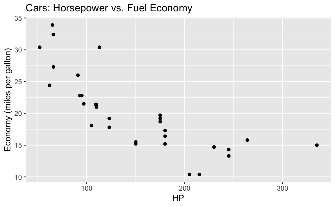
You want to change the background grid to your graphic.
With ggplot background grids come as a default, as you have seen in
other recipes. However we can alter the background grid using the
theme function or by applying a prepackaed theme to our graph.
We can use theme to alter the backgorund panel of our graphic:
ggplot(df)+geom_point(aes(x,y))+theme(panel.background=element_rect(fill="white",colour="grey50"))
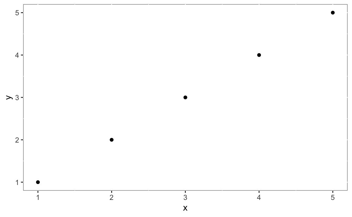
ggplot fills in the background with a grey grid by default. So you may
find yourself wanting to remove that grid completely or change it to
something else. Let’s create a ggplot graphic and then incrementally
change the background style.
We can add or change aspects of our graphic by creating a ggplot
object then calling the object and using the + to add to it. The
background shading in a ggplot graphic is actually 3 different graph
elements:
panel.grid.major:
These are white by default and heavy
panel.grid.minor:
These are white by default and light
panel.background:
This is the background that is grey by default
You can see these elements if you look carefully at the background of Figure 10-4:
If we set the background as element_blank() then the major and minor
grids are there but they are white on white so we can’t see them in
???:
g1<-ggplot(mtcars,aes(hp,mpg))+geom_point()+labs(title="Cars: Horsepower vs. Fuel Economy",x="HP",y="Economy (miles per gallon)")+theme(panel.background=element_blank())g1
. image::images/10_Graphics_files/figure-html/examplebackground-1.png[]
Notice in the code above we put the ggplot graph into a variable
called g1. Then we printed the graphic by just calling g1. By having
the graph inside of g1 we can then add additional graphical components
without rebuilding the graph again.
But if we wanted to show the background grid in some bright colors for illustration, it’s as easy as setting them to a color and setting a line type which is shown in ???.
g2<-g1+theme(panel.grid.major=element_line(color="red",linetype=3))+# linetype = 3 is dashtheme(panel.grid.minor=element_line(color="blue",linetype=4))# linetype = 4 is dot dashg2
. image::images/10_Graphics_files/figure-html/majorgrid-1.png[]
??? lacks visual appeal, but you can cleary see that the red lines make up the major grid and the blue lines are the minor grid.
Or we could do something less garash and take the ggplot object g1
from above and add grey gridlines to the white background, shown in
Figure 10-6.
g1+theme(panel.grid.major=element_line(colour="grey"))
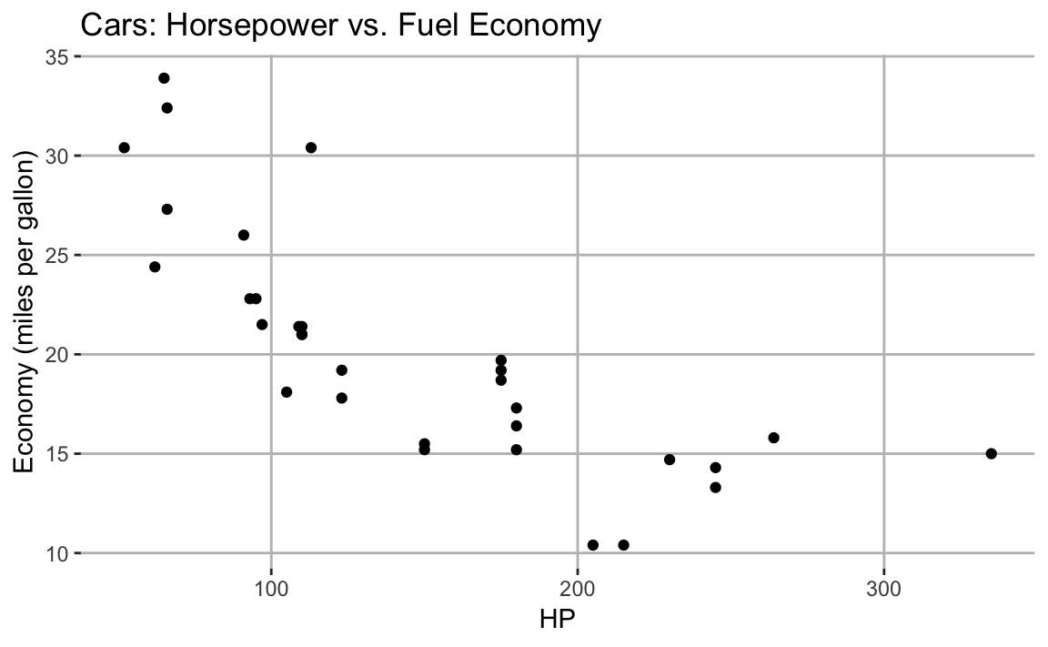
You have data in a data frame with three observations per record: x, y, and a factor f that indicates the group. You want to create a scatter plot of x and y that distinguishes among the groups.
With ggplot we control the mapping of shapes to the factor f by
passing shape = f to the aes.
ggplot(df,aes(x,y,shape=f))+geom_point()
Plotting multiple groups in one scatter plot creates an uninformative
mess unless we distinguish one group from another. This distinction is
done in ggplot by setting the shape parameter of the aes function.
The built in iris dataset contains paired measures of Petal.Length
and Petal.Width. Each measurement also has a Species property
indicating the species of the flower that was measured. If we plot all
the data at once, we just get the scatter plot shown in ???:
ggplot(data=iris,aes(x=Petal.Length,y=Petal.Width))+geom_point()
. image::images/10_Graphics_files/figure-html/irisnoshape-1.png[]
The graphic would be far more informative if we distinguished the points
by species. In addition to distinguising species by shape, we could also
differentiate by color. We can add shape = Species and
color = Species to our aes call, to get each species with a
different shape and color, shown in ???.
ggplot(data=iris,aes(x=Petal.Length,y=Petal.Width,shape=Species,color=Species))+geom_point()
. image::images/10_Graphics_files/figure-html/irisshape-1.png[]
ggplot conveniently sets up a legend for you as well, which is handy.
See “Adding (or Removing) a Legend” to add a legend.
You want your plot to include a legend, the little box that decodes the graphic for the viewer.
In most cases ggplot will add the legends automatically, as you can
see in the previous recipe. If you do not have explicit grouping in the
aes then ggplot will not show a legend by default. If we want to
force ggplot to show a legend we can set the shape or linetype of our
graph to a constant. ggplot will then show a legend with one group. We
then use guides to guide ggplot in how to label the legend.
This can be illustrated with our iris scatterplot:
g<-ggplot(data=iris,aes(x=Petal.Length,y=Petal.Width,shape="Point Name"))+geom_point()+guides(shape=guide_legend(title="Legend Title"))g
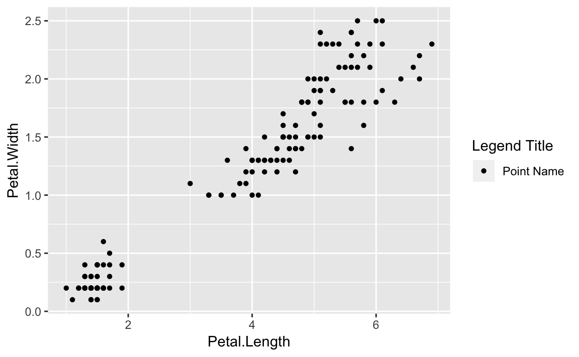
Figure 10-7 illustrates the result of setting the shape
to a string value then relabeling the legend using guides.
More commonly, you may want to turn legends off which can be done by
setting the legend.position = "none" in the theme. We can use the
iris plot from the prior recipe and add the theme call as shown in
Figure 10-8:
g<-ggplot(data=iris,aes(x=Petal.Length,y=Petal.Width,shape=Species,color=Species))+geom_point()+theme(legend.position="none")g
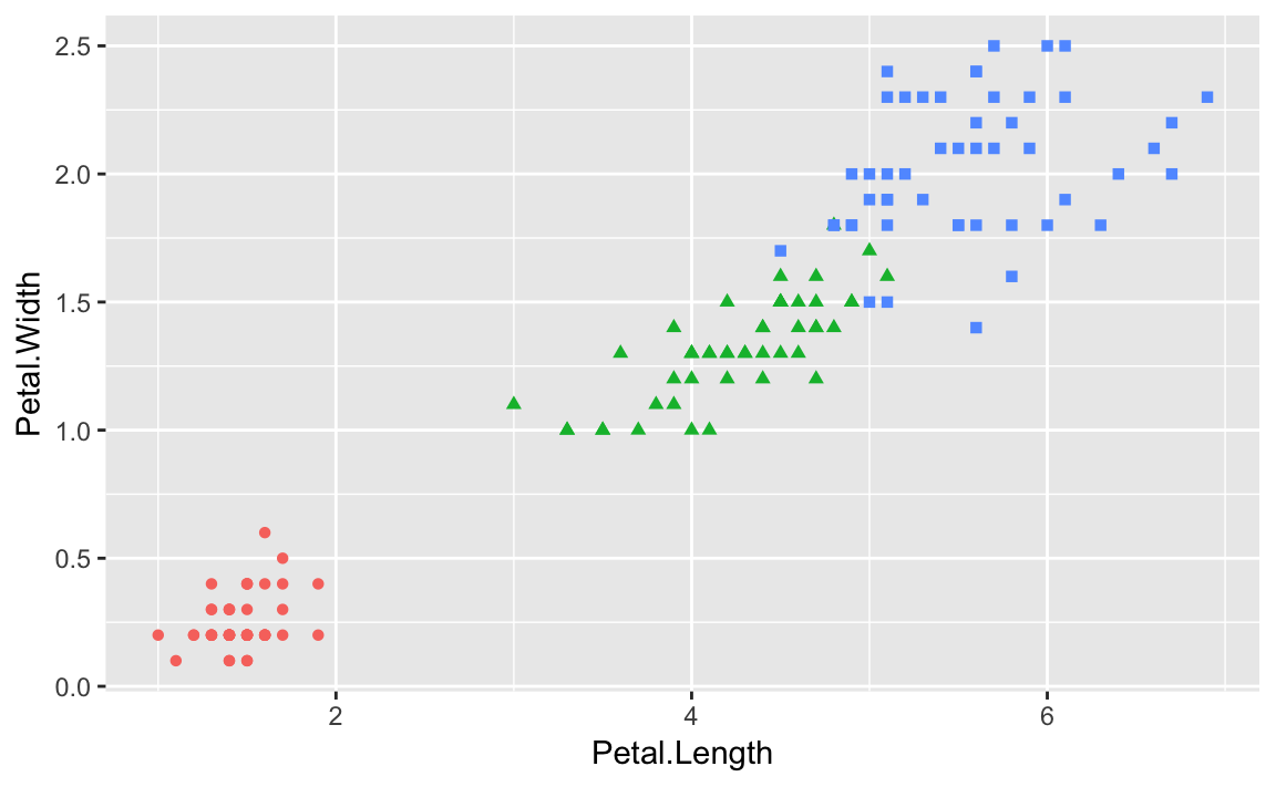
Adding legends to ggplot when there is no grouping is an excercise in
tricking ggplot into showing the legend by passing a string to a
grouping parameter in aes. This will not change the grouping as there
is only one group, but will result in a legend being shown with a name.
Then we can use guides to alter the legend title. It’s worth noting
that we are not changing anything about the data, just exploiting
settings in order to coerce ggplot into showing a legend when it
typically would not.
One of the huge benefits of ggplot is its very good defaults. Getting
positions and correspondence between labels and their point types is
done automatically, but can be overridden if needed. To remove a legend
totally, we set theme parameters with
theme(legend.position = "none"). In addition to “none” you can set the
legend.position to be "left", "right", "bottom", "top", or a
two-element numeric vector. Use a two-element numeric vector in order to
pass ggplot specific coordinates of where you want the legend. If
using the coordinate positions the values passed are between 0 and 1 for
x and y position, respectivly.
An example of a legend positioned at the bottom is in Figure 10-9 created with this adjustment to the
legend.poisition:
g+theme(legend.position="bottom")
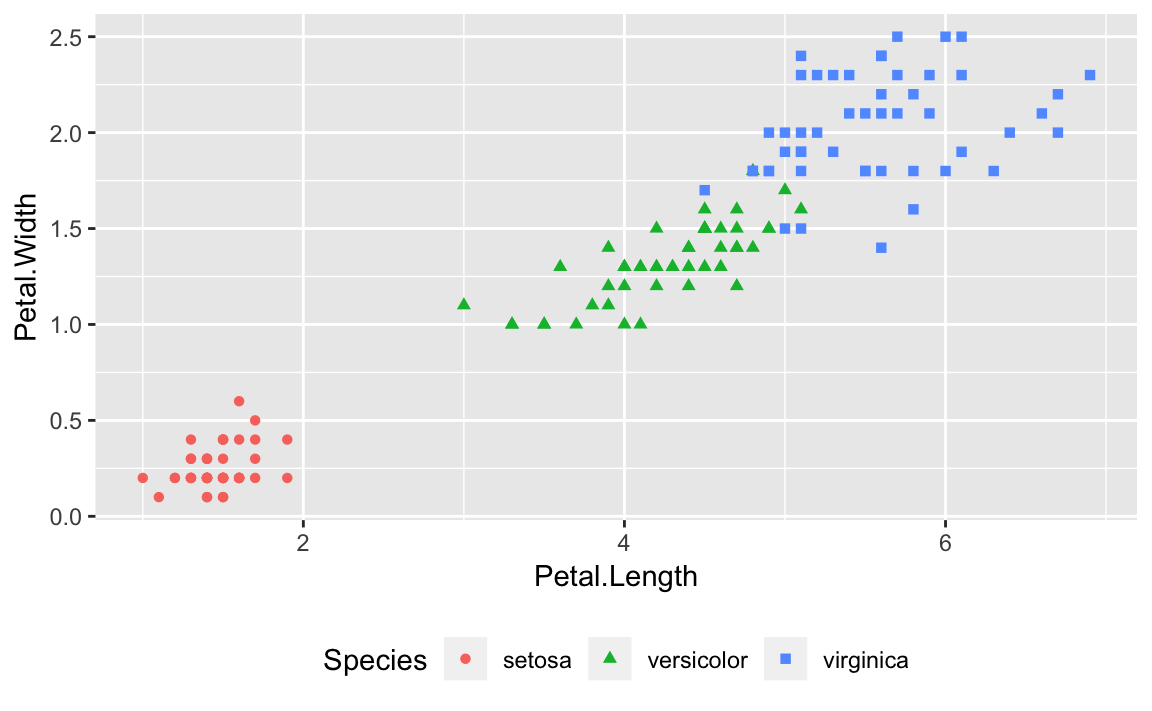
Or we could use the two-element numeric vector to put the legend in a specific location as in Figure 10-10. The example puts the center of the legend at 80% to the right and 20% up from the bottom.
g+theme(legend.position=c(.8,.2))
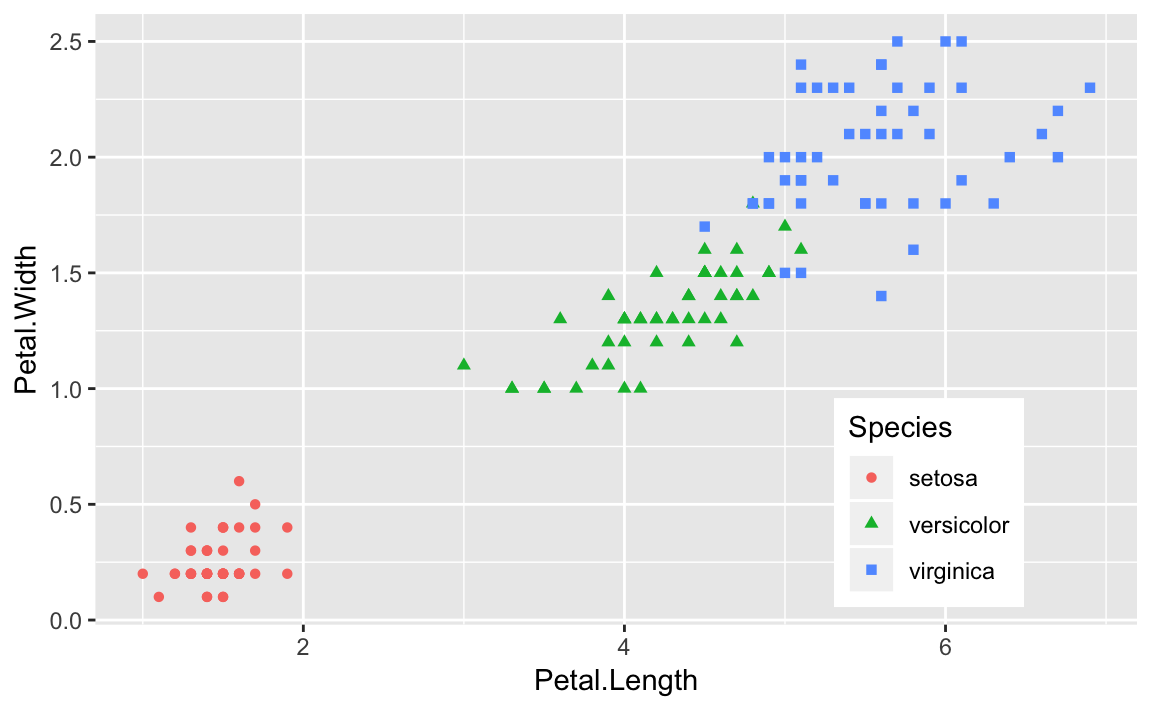
In many aspects beyond legends, ggplot uses sane defaults with
flexibility to override those and tweak the details. More detail of
ggplot options related to legends can be found in the help for theme
by typing ?theme or looking in the ggplot online reference material:
You are plotting pairs of data points, and you want to add a line that illustrates their linear regression.
Using ggplot there is no need to calculate the linear model first
using the R lm function. We can instead use the geom_smooth function
to calculate the linear regression inside of our ggplot call.
If our data is in a data frame df and the x and y data are in
columns x and y we plot the regression line like this:
ggplot(df,aes(x,y))+geom_point()+geom_smooth(method="lm",formula=y~x,se=FALSE)
The se = FALSE parameter tells ggplot not to plot the standard error
bands around our regression line.
Suppose we are modeling the strongx dataset found in the faraway
package. We can create a linear model using the built in lm function
in R. We can predict the variable crossx as a linear function of
energy. First, lets look at a simple scatter plot of our data:
library(faraway)data(strongx)ggplot(strongx,aes(energy,crossx))+geom_point()
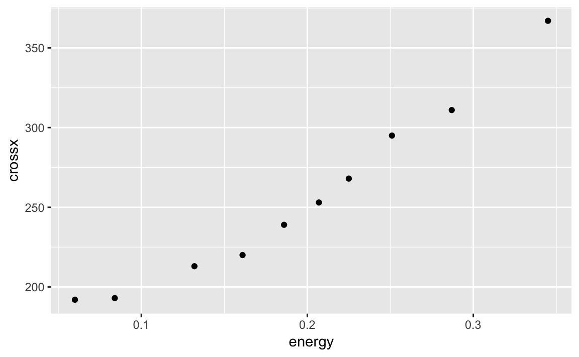
ggplot can calculate a linear model on the fly and then plot the
regression line along with our data:
g<-ggplot(strongx,aes(energy,crossx))+geom_point()g+geom_smooth(method="lm",formula=y~x,se=FALSE)
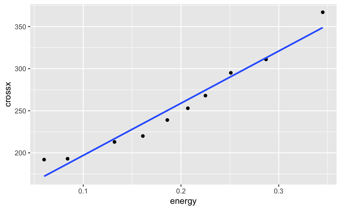
We can turn the confidence bands on by omitting the se = FALSE option
as as shown in ???:
g+geom_smooth(method="lm",formula=y~x)
. image::images/10_Graphics_files/figure-html/one-step-nose-1.png[]
Notice that in the geom_smooth we use x and y rather than the
variable names. ggplot has set the x and y inside the plot based
on the aesthetic. Multiple smoothing methods are supported by
geom_smooth. You can explore those, and other options in the help by
typing ?geom_smooth.
If we had a line we wanted to plot that was stored in another R object,
we could use geom_abline to plot the line on our graph. In the
following example we pull the intercept term and the slope from the
regression model m and add those to our graph:
m<-lm(crossx~energy,data=strongx)ggplot(strongx,aes(energy,crossx))+geom_point()+geom_abline(intercept=m$coefficients[1],slope=m$coefficients[2])
This produces a very similar plot to ???. The
geom_abline method can be handy if you are plotting a line from a
source other than a simple linear model.
See the chapter on Linear Regression and
ANOVA for more about linear regression and the lm function.
Your dataset contains multiple numeric variables. You want to see scatter plots for all pairs of variables.
ggplot does not have any built in method to create pairs plots,
however, the package GGally provides the functionality with the
ggpairs function:
library(GGally)ggpairs(df)
When you have a large number of variables, finding interrelationships
between them is difficult. One useful technique is looking at scatter
plots of all pairs of variables. This would be quite tedious if coded
pair-by-pair, but the ggpairs function from the package GGally
provides an easy way to produce all those scatter plots at once.
The iris dataset contains four numeric variables and one categorical
variable:
head(iris)#> Sepal.Length Sepal.Width Petal.Length Petal.Width Species#> 1 5.1 3.5 1.4 0.2 setosa#> 2 4.9 3.0 1.4 0.2 setosa#> 3 4.7 3.2 1.3 0.2 setosa#> 4 4.6 3.1 1.5 0.2 setosa#> 5 5.0 3.6 1.4 0.2 setosa#> 6 5.4 3.9 1.7 0.4 setosa
What is the relationship, if any, between the columns? Plotting the
columns with ggpairs produces multiple scatter plots.
library(GGally)ggpairs(iris)
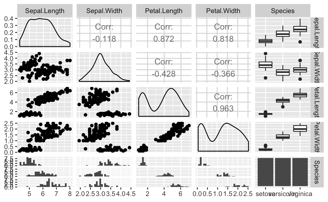
ggpairs Plot of Iris DataThe ggpairs function is pretty, but not particularly fast. If you’re
just doing interactive work and want a quick peak at the data, the base
R plot function provides faster output and is shown in Figure 10-13.
plot(iris)
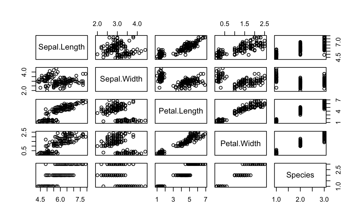
While the ggpairs function is not as fast to plot as the Base R plot
function, it produces density graphs on the diagonal and reports
correlation in the upper triangle of the graph. When factors or
character columns are present, ggpairs produces histograms on the
lower triangle of the graph and boxplots on the upper triangle. These
are nice additions to understanding relationships in your data.
Your dataset contains (at least) two numeric variables and a factor. You want to create several scatter plots for the numeric variables, with one scatter plot for each level of the factor.
This kind of plot is called a conditioning plot, which is produced in
ggplot by adding facet_wrap to our plot. In this example we use the
data frame df which contains three columns: x, y, and f with f
being a factor (or a character).
ggplot(df,aes(x,y))+geom_point()+facet_wrap(~f)
Conditioning plots (coplots) are another way to explore and illustrate the effect of a factor or to compare different groups to each other.
The Cars93 dataset contains 27 variables describing 93 car models as
of 1993. Two numeric variables are MPG.city, the miles per gallon in
the city, and Horsepower, the engine horsepower. One categorical
variable is Origin, which can be USA or non-USA according to where the
model was built.
Exploring the relationship between MPG and horsepower, we might ask: Is there a different relationship for USA models and non-USA models?
Let’s examine this as a facet plot:
data(Cars93,package="MASS")ggplot(data=Cars93,aes(MPG.city,Horsepower))+geom_point()+facet_wrap(~Origin)
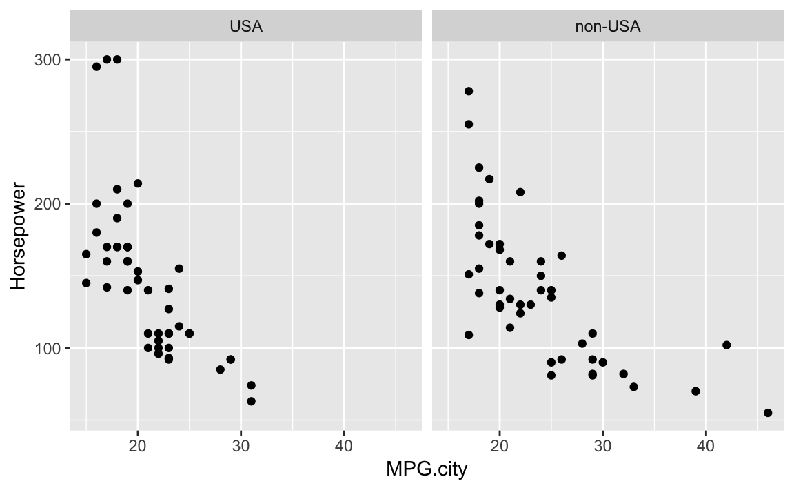
The resulting plot in Figure 10-13 reveals a few insights. If we really crave that 300-horsepower monster then we’ll have to buy a car built in the USA; but if we want high MPG, we have more choices among non-USA models. These insights could be teased out of a statistical analysis, but the visual presentation reveals them much more quickly.
Note that using facet results in subplots with the same x and y
axis ranges. This helps insure that visual inspection of the data is not
misleading because of differeing axis ranges.
The Base R Graphics function coplot can accomplish very similar plots
using only Base Graphics.
You want to create a bar chart.
A common situation is to have a column of data that represents a group and then another column that represents a measure about that group. This format is “long” data because the data runs vertically instead of having a column for each group.
Using the geom_bar function in ggplot we can plot the heights as
bars. If the data is already aggregated, we add stat = "identity" so
that ggplot knows it needs to do no aggregation on the groups of
values before plotting.
ggplot(data=df,aes(x,y))+geom_bar(stat="identity")
Let’s use the cars made by Ford in the Cars93 data in an example:
ford_cars<-Cars93%>%filter(Manufacturer=="Ford")ggplot(ford_cars,aes(Model,Horsepower))+geom_bar(stat="identity")
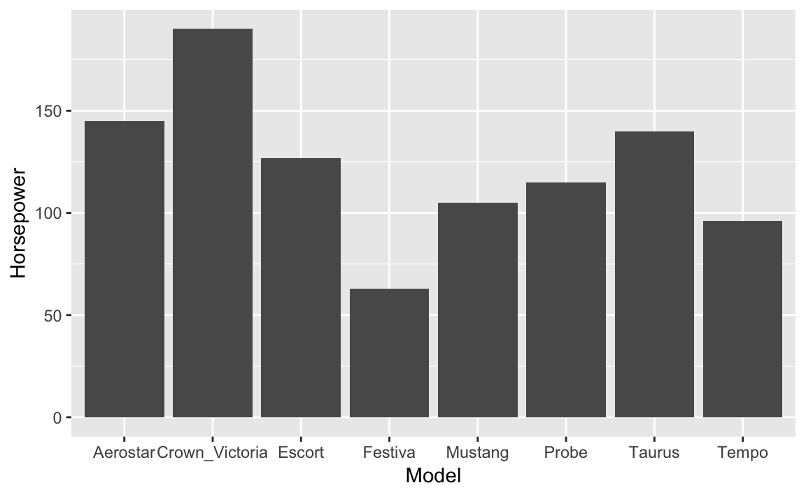
The resulting graph in Figure 10-15 shows the resuting bar chart.
This example above uses stat = "identity" which assumes that the
heights of your bars are conveniently stored as a value in one field
with only one record per column. That is not always the case, however.
Often you have a vector of numeric data and a parallel factor or
character field that groups the data, and you want to produce a bar
chart of the group means or the group totals.
Let’s work up an example using the built-in airquality dataset which
contains daily temperature data for a single location for five months.
The data frame has a numeric Temp column and Month and Day
columns. If we want to plot the mean temp by month using ggplot we
don’t need to precompute the mean, instead we can have ggplot do that
in the plot command logic. To tell ggplot to calculate the mean we
pass stat = "summary", fun.y = "mean" to the geom_bar command. We
can also turn the month numbers into dates using the built in constant
month.abb which contains the abbreviations for the months.
ggplot(airquality,aes(month.abb[Month],Temp))+geom_bar(stat="summary",fun.y="mean")+labs(title="Mean Temp by Month",x="",y="Temp (deg. F)")
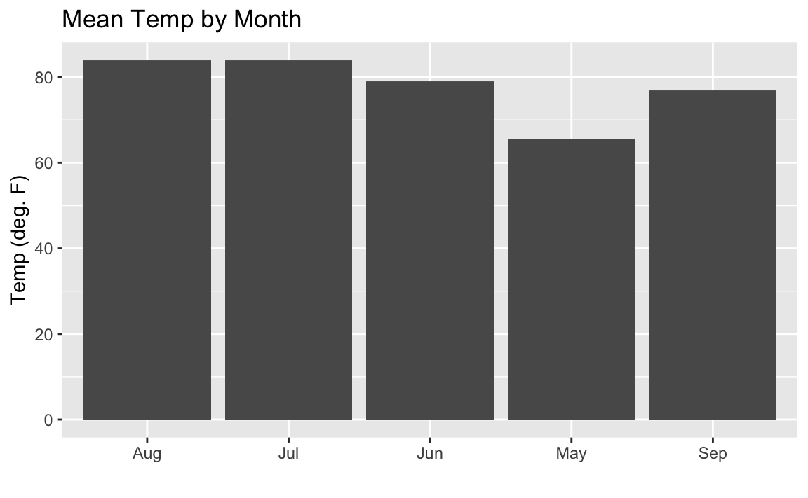
Figure 10-16 shows the resulting plot. But you might notice the sort order on the months is alphabetical, which is not how we typically like to see months sorted.
We can fix the sorting issue using a few functions from dplyr combined
with fct_inorder from the forcats Tidyverse package. To get the
months in the correct order we can sort the data frame by Month which
is the month number, then we can apply fct_inorder which will arrange
our factors in the order they appear in the data. You can see in Figure 10-17 that the bars are now sorted properly.
aq_data<-airquality%>%arrange(Month)%>%mutate(month_abb=fct_inorder(month.abb[Month]))ggplot(aq_data,aes(month_abb,Temp))+geom_bar(stat="summary",fun.y="mean")+labs(title="Mean Temp by Month",x="",y="Temp (deg. F)")
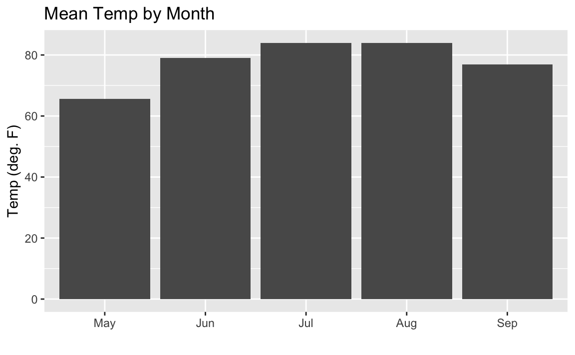
See “Adding Confidence Intervals to a Bar Chart” for adding confidence intervals and “Coloring a Bar Chart” for adding color
?geom_bar for help with bar charts in ggplot
barplot for Base R bar charts or the barchart function in the
lattice package.
You want to augment a bar chart with confidence intervals.
Suppose you have a data frame df with columns group which are group
names, stat which is a column of statistics, and lower and upper
which represent the corresponding limits for the confidence intervals.
We can display a bar chart of stat for each group and its confidence
intervals using the geom_bar combined with geom_errorbar.
ggplot(df,aes(group,stat))+geom_bar(stat="identity")+geom_errorbar(aes(ymin=lower,ymax=upper),width=.2)
. image::images/10_Graphics_files/figure-html/confbars-1.png[]
??? shows the resulting bar chart with confidence intervals.
Most bar charts display point estimates, which are shown by the heights of the bars, but rarely do they include confidence intervals. Our inner statisticians dislike this intensely. The point estimate is only half of the story; the confidence interval gives the full story.
Fortunately, we can plot the error bars using ggplot. The hard part is
calculating the intervals. In the examples above our data had a simple
-15% and +20% interval. However, in “Creating a Bar Chart”, we calculated group means before plotting them. If we let
ggplot do the calculations for us we can use the build in mean_se
along with the stat_summary function to get the standard errors of the
mean measures.
Let’s use the airquality data we used previously. First we’ll do the
sorted factor procedure (from the prior recipe) to get the month names
in the desired order:
aq_data<-airquality%>%arrange(Month)%>%mutate(month_abb=fct_inorder(month.abb[Month]))
Now we can plot the bars along with the associated standard errors as in the following:
ggplot(aq_data,aes(month_abb,Temp))+geom_bar(stat="summary",fun.y="mean",fill="cornflowerblue")+stat_summary(fun.data=mean_se,geom="errorbar")+labs(title="Mean Temp by Month",x="",y="Temp (deg. F)")
Sometimes you’ll want to sort your columns in your bar chart in
descending order based on their height. This can be a little bit
confusing when using summary stats in ggplot but the secret is to use
mean in the reorder statement to sort the factor by the mean of the
temp. Note that the reference to mean in reorder is not quoted,
while the reference to mean in geom_bar is quoted:
ggplot(aq_data,aes(reorder(month_abb,-Temp,mean),Temp))+geom_bar(stat="summary",fun.y="mean",fill="tomato")+stat_summary(fun.data=mean_se,geom="errorbar")+labs(title="Mean Temp by Month",x="",y="Temp (deg. F)")
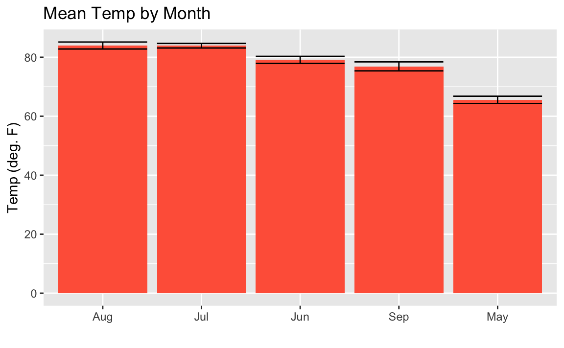
You may look at this example and the result in Figure 10-18
and wonder, “Why didn’t they just use reorder(month_abb, Month) in the
first example instead of that sorting business with
forcats::fct_inorder to get the months in the right order?” Well, we
could have. But sorting using fct_inorder is a design pattern that
provides flexibility for more complicated things. Plus it’s quite easy
to read in a script. Using reorder inside the aes is a bit more
dense and hard to read later. But either approach is reasonable.
See “Forming a Confidence Interval for a Mean” for
more about t.test.
You want to color or shade the bars of a bar chart.
With gplot we add the fill= call to our aes and let ggplot pick
the colors for us:
ggplot(df,aes(x,y,fill=group))
In ggplot we can use the fill parameter in aes to tell ggplot
what field to base the colors on. If we pass a numeric field to ggplot
we will get a continuous gradient of colors and if we pass a factor or
character field to fill we will get contrasting colors for each group.
Below we pass the character name of each month to the fill parameter:
aq_data<-airquality%>%arrange(Month)%>%mutate(month_abb=fct_inorder(month.abb[Month]))ggplot(data=aq_data,aes(month_abb,Temp,fill=month_abb))+geom_bar(stat="summary",fun.y="mean")+labs(title="Mean Temp by Month",x="",y="Temp (deg. F)")+scale_fill_brewer(palette="Paired")
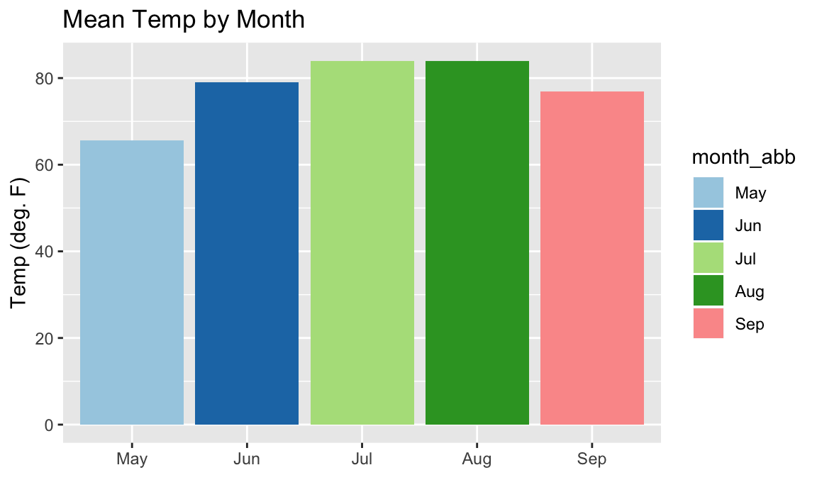
The colors in the resulting Figure 10-19 are defined by
calling scale_fill_brewer(palette="Paired"). The "Paired" color
palette comes, along with many other color pallets, in the package
RColorBrewer.
If we wanted to change the color of each bar based on the temperature,
we can’t just set fill=Temp as might seem intuitive because ggplot
would not understand we want the mean temperature after the grouping by
month. So the way we get around this is to access a special field inside
of our graph called ..y.. which is the calculated value on the Y axis.
But we don’t want the legend labeled ..y.. so we add fill="Temp" to
our labs call in order to change the name of the legend. The result is
???
ggplot(airquality,aes(month.abb[Month],Temp,fill=..y..))+geom_bar(stat="summary",fun.y="mean")+labs(title="Mean Temp by Month",x="",y="Temp (deg. F)",fill="Temp")
images::images/10_Graphics_files/figure-latex/barsshaded-1.png[]
If we want to reverse the color scale, we can just add a negative - in
front of the field we are filling by. Like fill= -..y.., for example.
See “Creating a Bar Chart” for creating a bar chart.
You have paired observations in a data frame: (x1, y1), (x2, y2), …, (xn, yn). You want to plot a series of line segments that connect the data points.
With ggplot we can use geom_point to plot the points:.
ggplot(df,aes(x,y))+geom_point()
Since ggplot graphics are built up, element by element, we can have
both a point and a line in the same graphic very easily by having two
geoms:
ggplot(df,aes(x,y))+geom_point()+geom_line()
To illustrate, let’s look at some example US economic data that comes
with ggplot2. This example data frame has a column called date which
we’ll plot on the x axis and a field unemploy which is the number of
unemployed people.
ggplot(economics,aes(date,unemploy))+geom_point()+geom_line()
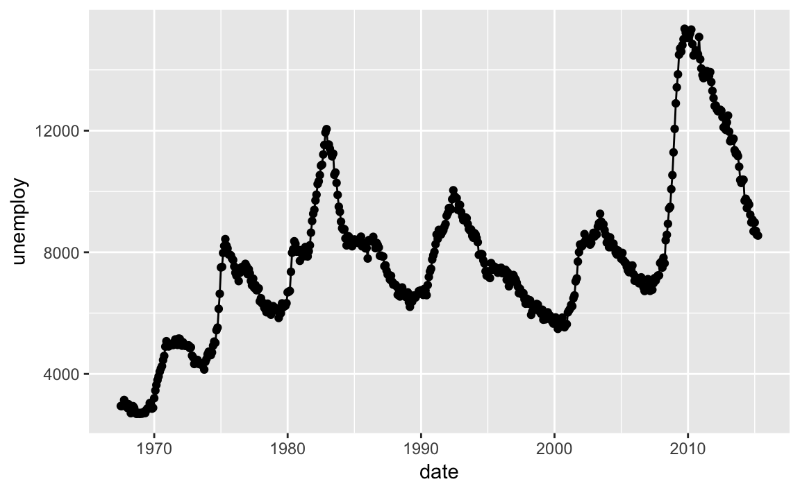
Figure 10-20 shows the resulting chart which contains both lines and points because we used both geoms.
You are plotting a line. You want to change the type, width, or color of the line.
ggplot uses the linetype parameter for controlling the appearance of
lines:
linetype="solid" or linetype=1 (default)
linetype="dashed" or linetype=2
linetype="dotted" or linetype=3
linetype="dotdash" or linetype=4
linetype="longdash" or linetype=5
linetype="twodash" or linetype=6
linetype="blank" or linetype=0 (inhibits drawing)
You can change the line characteristics by passing linetype, col
and/or size as parameters to the geom_line. So if we want to change
the linetype to dashed, red, and heavy we could pass the linetype,
col and size params to geom_line:
ggplot(df,aes(x,y))+geom_line(linetype=2,size=2,col="red")
The example syntax above shows how to draw one line and specify its style, width, or color. A common scenario involves drawing multiple lines, each with its own style, width, or color.
Let’s set up some example data:
x<-1:10y1<-x**1.5y2<-x**2y3<-x**2.5df<-data.frame(x,y1,y2,y3)
In ggplot this can be a conundrum for many users. The challenge is
that ggplot works best with “long” data instead of “wide” data as was
mentioned in the introduction to this chapter. Our example data frame
has 4 columns of wide data:
head(df,3)#> x y1 y2 y3#> 1 1 1.00 1 1.00#> 2 2 2.83 4 5.66#> 3 3 5.20 9 15.59
We can make our wide data long by using the gather function from the
core tidyverse pacakge tidyr. In the example below, we use gather to
create a new column named bucket and put our column names in there
while keeping our x and y variables.
df_long<-gather(df,bucket,y,-x)head(df_long,3)#> x bucket y#> 1 1 y1 1.00#> 2 2 y1 2.83#> 3 3 y1 5.20tail(df_long,3)#> x bucket y#> 28 8 y3 181#> 29 9 y3 243#> 30 10 y3 316
Now we can pass bucket to the col parameter and get multiple lines,
each a different color:
ggplot(df_long,aes(x,y,col=bucket))+geom_line()
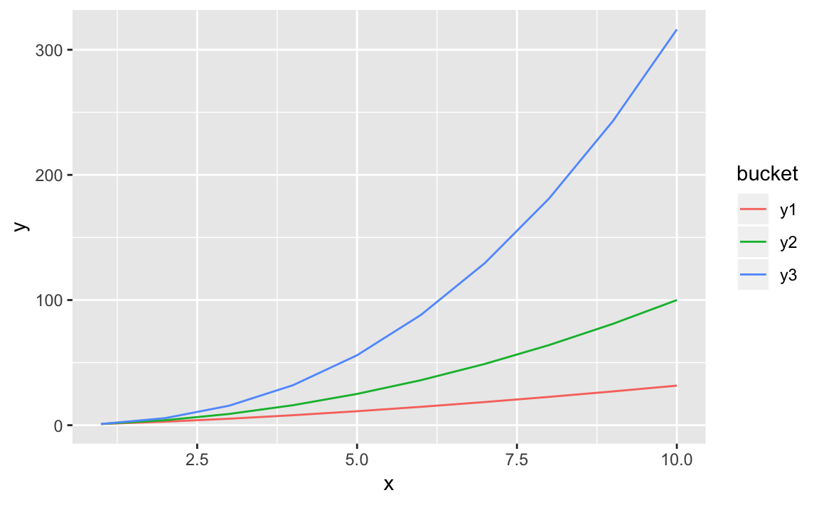
It’s straight forward to vary the line weight by a variable by passing a
numerical variable to size:
ggplot(df,aes(x,y1,size=y2))+geom_line()+scale_size(name="Thickness based on y2")
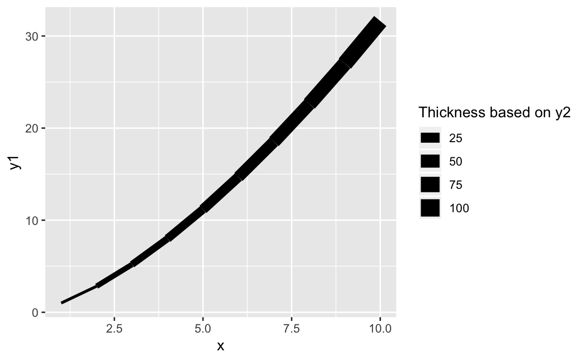
The result of varying the thickness with x is shown in Figure 10-21.
See “Plotting a Line from x and y Points” for plotting a basic line.
You want to show multiple datasets in one plot.
We could combine the data into one data frame before plotting using one
of the join functions from dplyr. However below we will create two
seperate data frames then add them each to a ggplot graph.
First let’s set up our example data frames, df1 and df2:
# example datan<-20x1<-1:ny1<-rnorm(n,0,.5)df1<-data.frame(x1,y1)x2<-(.5*n):((1.5*n)-1)y2<-rnorm(n,1,.5)df2<-data.frame(x2,y2)
Typically we would pass the data frame directly into the ggplot
function call. Since we want two geoms with two different data sources,
we will initiate a plot with ggplot() and then add in two calls to
geom_line each with its own data source.
ggplot()+geom_line(data=df1,aes(x=x1,y=y1),color="darkblue")+geom_line(data=df2,aes(x=x2,y=y2),linetype="dashed")
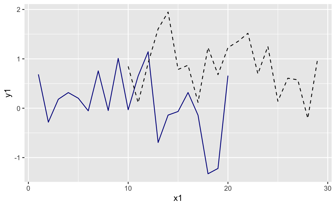
ggplot allows us to make multiple calls to different geom_ functions
each with its own data source, if desired. Then ggplot will look at
all the data we are plotting and adjust the ranges to accomodate all the
data.
Even with good defaults, sometimes we want our plot range to show a
different range. We can do that by setting the xlim and ylim in our
ggplot.
ggplot()+geom_line(data=df1,aes(x=x1,y=y1),color="darkblue")+geom_line(data=df2,aes(x=x2,y=y2),linetype="dashed")+xlim(0,35)+ylim(-2,2)
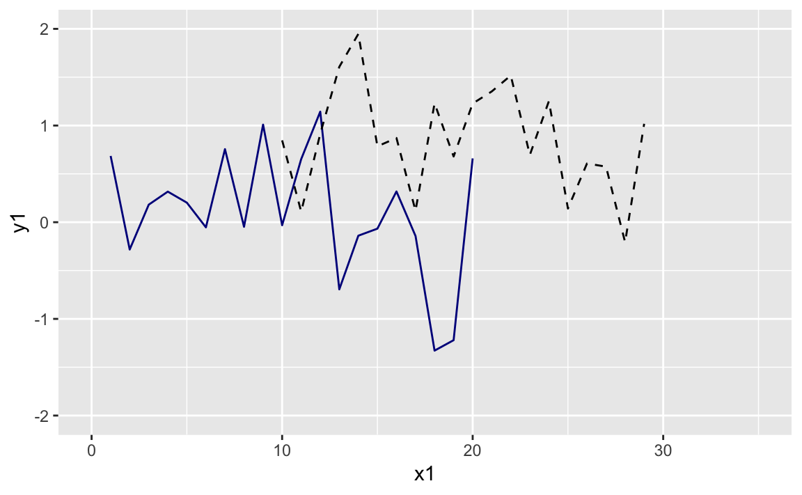
The graph with expanded limits is in Figure 10-23.
You want to add a vertical or horizontal line to your plot, such as an axis through the origin or pointing out a threshold.
The ggplot functions geom_vline and geom_hline allow vertical and
horizontal lines, respectivly. The functions can also take color,
linetype, and size parameters to set the line style:
# using the data.frame df1 from the prior recipeggplot(df1)+aes(x=x1,y=y1)+geom_point()+geom_vline(xintercept=10,color="red",linetype="dashed",size=1.5)+geom_hline(yintercept=0,color="blue")
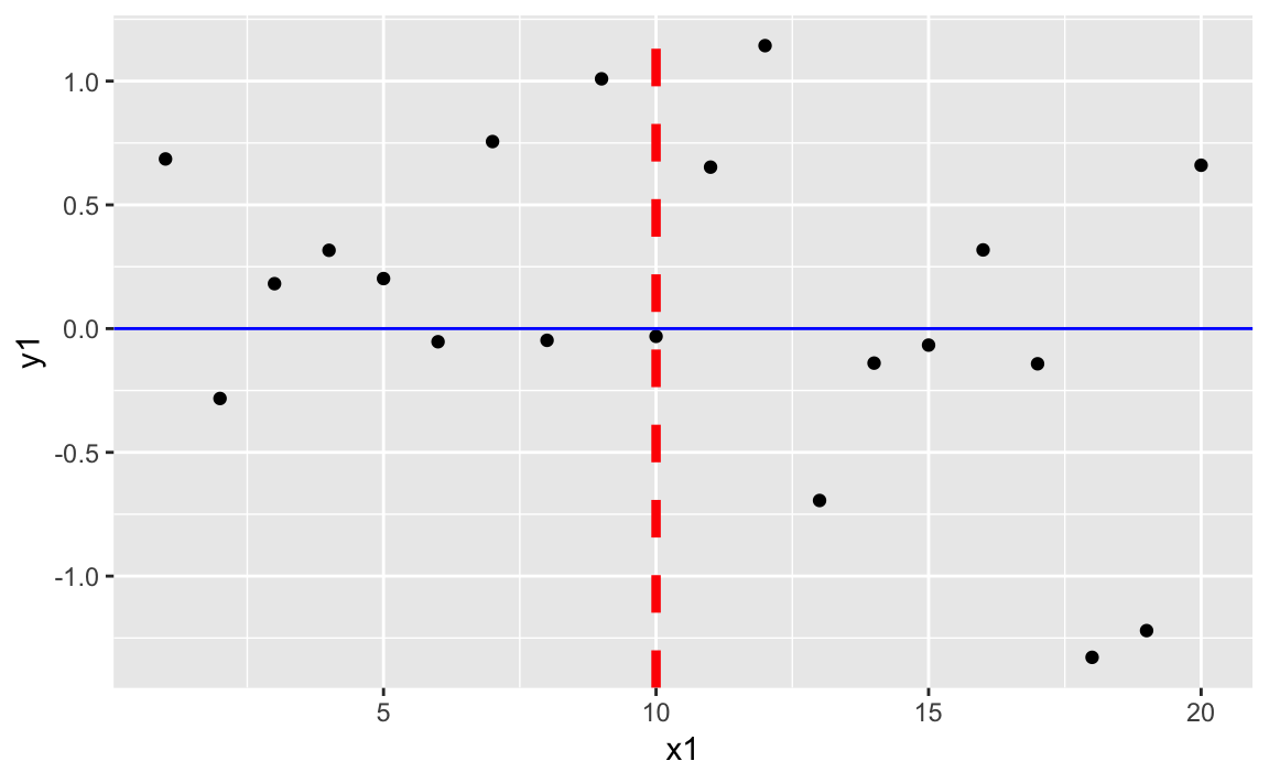
Figure 10-24 shows the resulting plot with added horizontal and vertical lines.
A typical use of lines would be drawing regularly spaced lines. Suppose
we have a sample of points, samp. First, we plot them with a solid
line through the mean. Then we calculate and draw dotted lines at ±1 and
±2 standard deviations away from the mean. We can add the lines into our
plot with geom_hline:
samp<-rnorm(1000)samp_df<-data.frame(samp,x=1:length(samp))mean_line<-mean(samp_df$samp)sd_lines<-mean_line+c(-2,-1,+1,+2)*sd(samp_df$samp)ggplot(samp_df)+aes(x=x,y=samp)+geom_point()+geom_hline(yintercept=mean_line,color="darkblue")+geom_hline(yintercept=sd_lines,linetype="dotted")
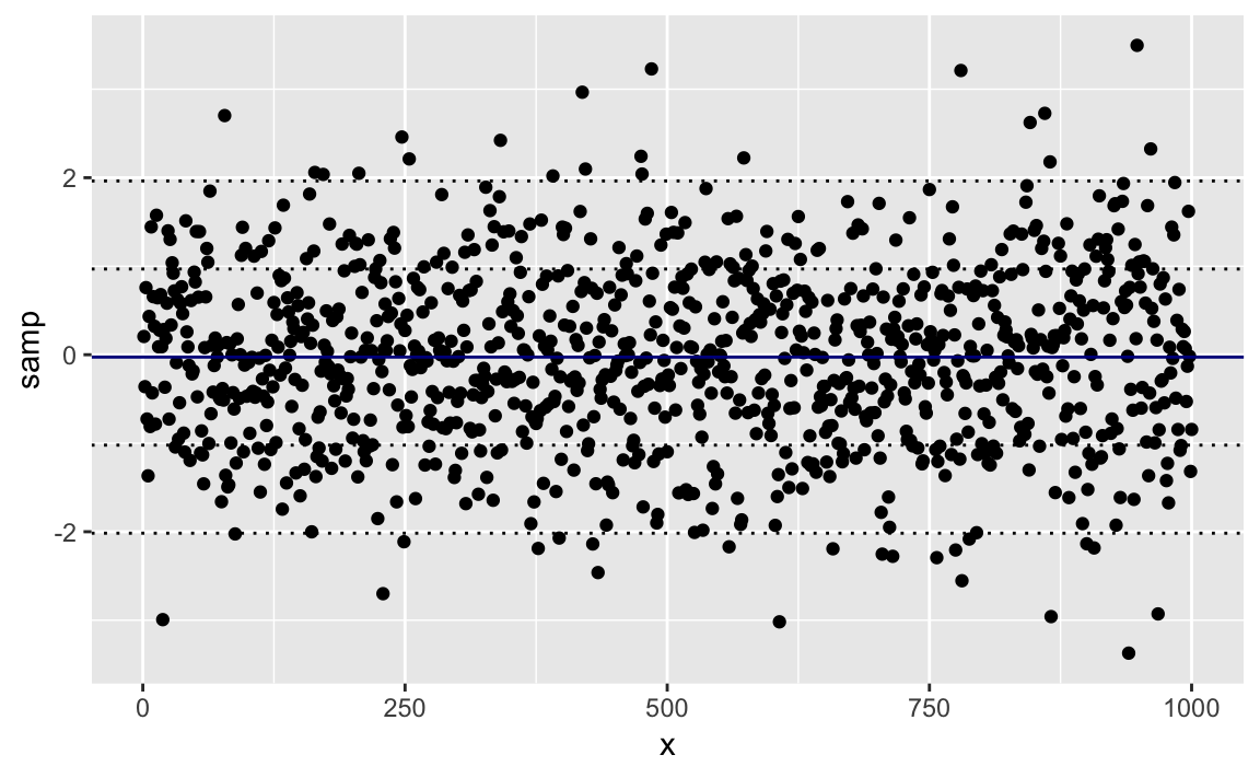
Figure 10-25 shows the sampled data along with the mean and standard deviation lines.
See “Changing the Type, Width, or Color of a Line” for more about changing line types.
You want to create a box plot of your data.
Use geom_boxplot from ggplot to add a boxplot geom to a ggplot
graphic. Using the samp_df data frame from the prior recipe, we can
create a box plot of the values in the x column. The resulting graph
is in Figure 10-26.
ggplot(samp_df)+aes(y=samp)+geom_boxplot()
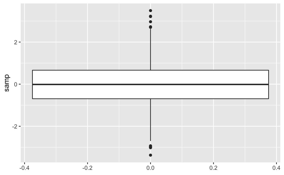
A box plot provides a quick and easy visual summary of a dataset.
The thick line in the middle is the median.
The box surrounding the median identifies the first and third quartiles; the bottom of the box is Q1, and the top is Q3.
The “whiskers” above and below the box show the range of the data, excluding outliers.
The circles identify outliers. By default, an outlier is defined as any value that is farther than 1.5 × IQR away from the box. (IQR is the interquartile range, or Q3 − Q1.) In this example, there are a few outliers on the high side.
We can rotate the boxplot by flipping the coordinates. There are some situations where this makes a more appealing graphic. This is shown in Figure 10-27.
ggplot(samp_df)+aes(y=samp)+geom_boxplot()+coord_flip()
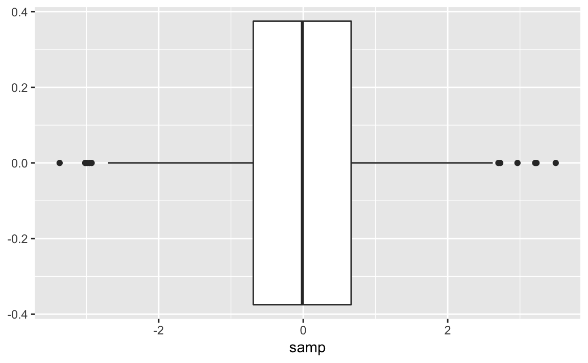
One box plot alone is pretty boring. See “Creating One Box Plot for Each Factor Level” for creating multiple box plots.
Your dataset contains a numeric variable and a factor (or other catagorical text). You want to create several box plots of the numeric variable broken out by levels.
With ggplot we pass the name of the categorical variable to the x
parameter in the aes call. The resulting boxplot will then be grouped
by the values in the categorical variable:
ggplot(df)+aes(x=factor,y=values)+geom_boxplot()
This recipe is another great way to explore and illustrate the relationship between two variables. In this case, we want to know whether the numeric variable changes according to the level of a category.
The UScereal dataset from the MASS package contains many variables
regarding breakfast cereals. One variable is the amount of sugar per
portion and another is the shelf position (counting from the floor).
Cereal manufacturers can negotiate for shelf position, placing their
product for the best sales potential. We wonder: Where do they put the
high-sugar cereals? We can produce Figure 10-28 and
explore that question by creating one box plot per shelf:
data(UScereal,package="MASS")ggplot(UScereal)+aes(x=as.factor(shelf),y=sugars)+geom_boxplot()+labs(title="Sugar Content by Shelf",x="Shelf",y="Sugar (grams per portion)")
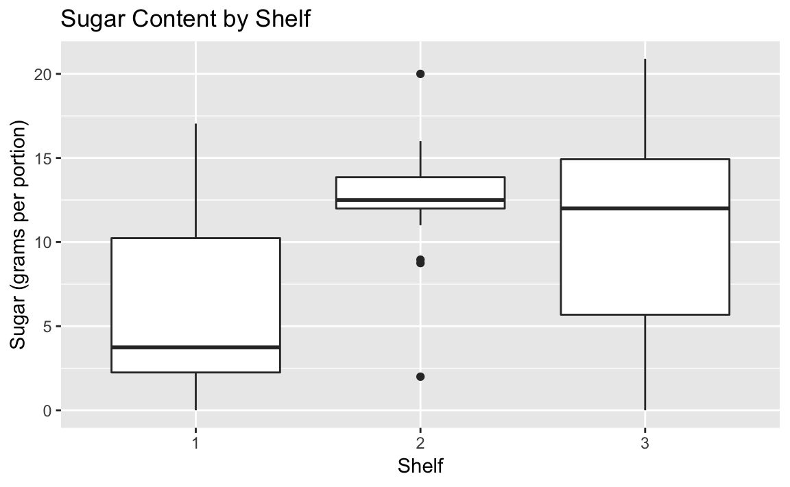
The box plots suggest that shelf #2 has the most high-sugar cereals. Could it be that this shelf is at eye level for young children who can influence their parent’s choice of cereals?
Note that in the aes call we had to tell ggplot to treat the shelf
number as a factor. Otherwise ggplot would not react to the shelf as a
grouping and only print a single boxplot.
See “Creating a Box Plot” for creating a basic box plot.
You want to create a histogram of your data.
Use geom_histogram, and set x to a vector of numeric values.
Figure 10-29 is a histogram of the MPG.city column taken
from the Cars93 dataset:
data(Cars93,package="MASS")ggplot(Cars93)+geom_histogram(aes(x=MPG.city))#> `stat_bin()` using `bins = 30`. Pick better value with `binwidth`.
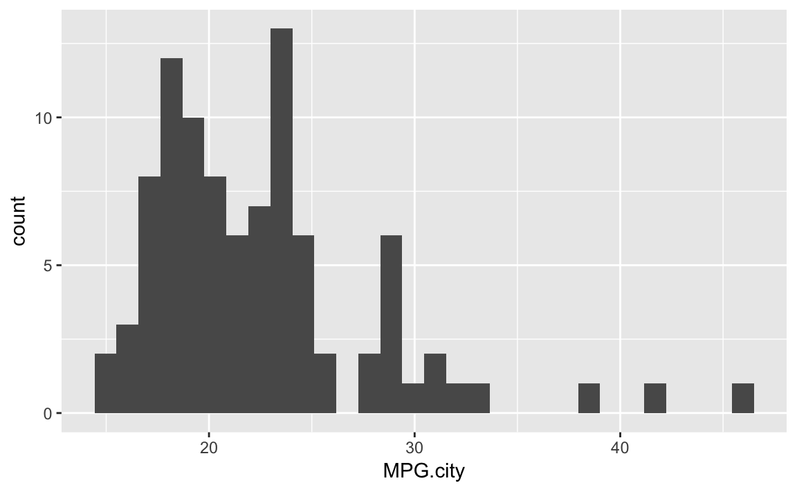
The geom_histogram function must decide how many cells (bins) to
create for binning the data. In this example, the default algorithm
chose 30 bins. If we wanted fewer bins, we wo would include the bins
parameter to tell geom_histogram how many bins we want:
ggplot(Cars93)+geom_histogram(aes(x=MPG.city),bins=13)
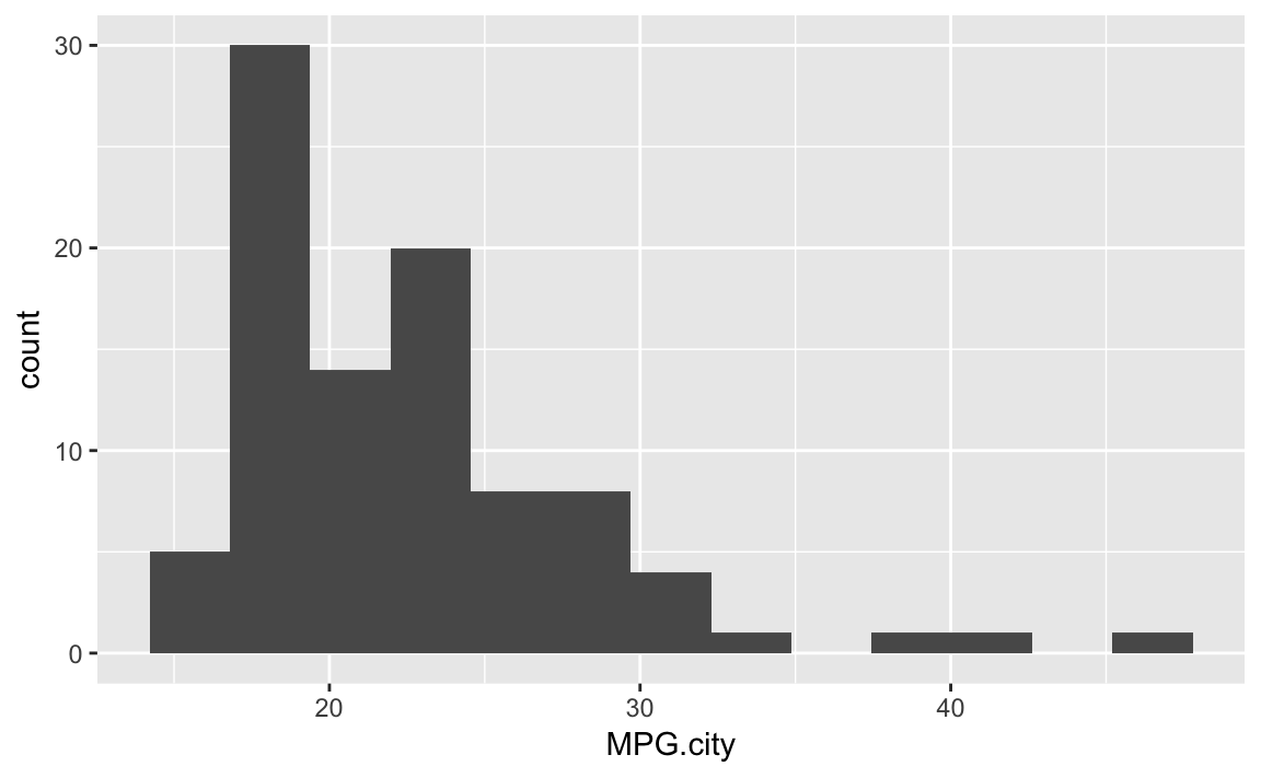
Figure 10-30 shows the histogram with 13 bins.
The Base R function hist provides much of the same functionality as
does the histogram function of the lattice package.
You have a histogram of your data sample, and you want to add a curve to illustrate the apparent density.
Use the geom_density function to approximate the sample density as
shown in Figure 10-31:
ggplot(Cars93)+aes(x=MPG.city)+geom_histogram(aes(y=..density..),bins=21)+geom_density()
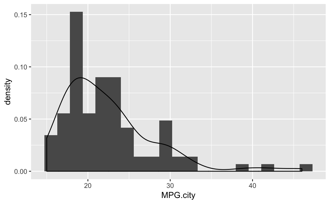
A histogram suggests the density function of your data, but it is rough. A smoother estimate could help you better visualize the underlying distribution. A Kernel Density Estimation (KDE) is a smoother representation of univariate data.
In ggplot we tell the geom_histogram function to use the density
function by passing it aes(y = ..density..).
The following example takes a sample from a gamma distribution and then plots the histogram and the estimated density as shown in Figure 10-32.
samp<-rgamma(500,2,2)ggplot()+aes(x=samp)+geom_histogram(aes(y=..density..),bins=10)+geom_density()
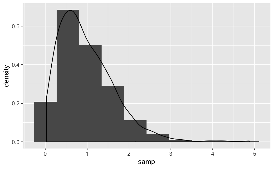
The density function approximates the shape of the density nonparametrically. If you know the actual underlying distribution, use instead “Plotting a Density Function” to plot the density function.
You want to create a quantile-quantile (Q-Q) plot of your data, typically because you want to know how the data differs from a normal distribution.
With ggplot we can use the stat_qq and stat_qq_line functions to
create a Q-Q plot that shows both the observed points as well as the Q-Q
Line. Figure 10-33 shows the resulting plot.
df<-data.frame(x=rnorm(100))ggplot(df,aes(sample=x))+stat_qq()+stat_qq_line()
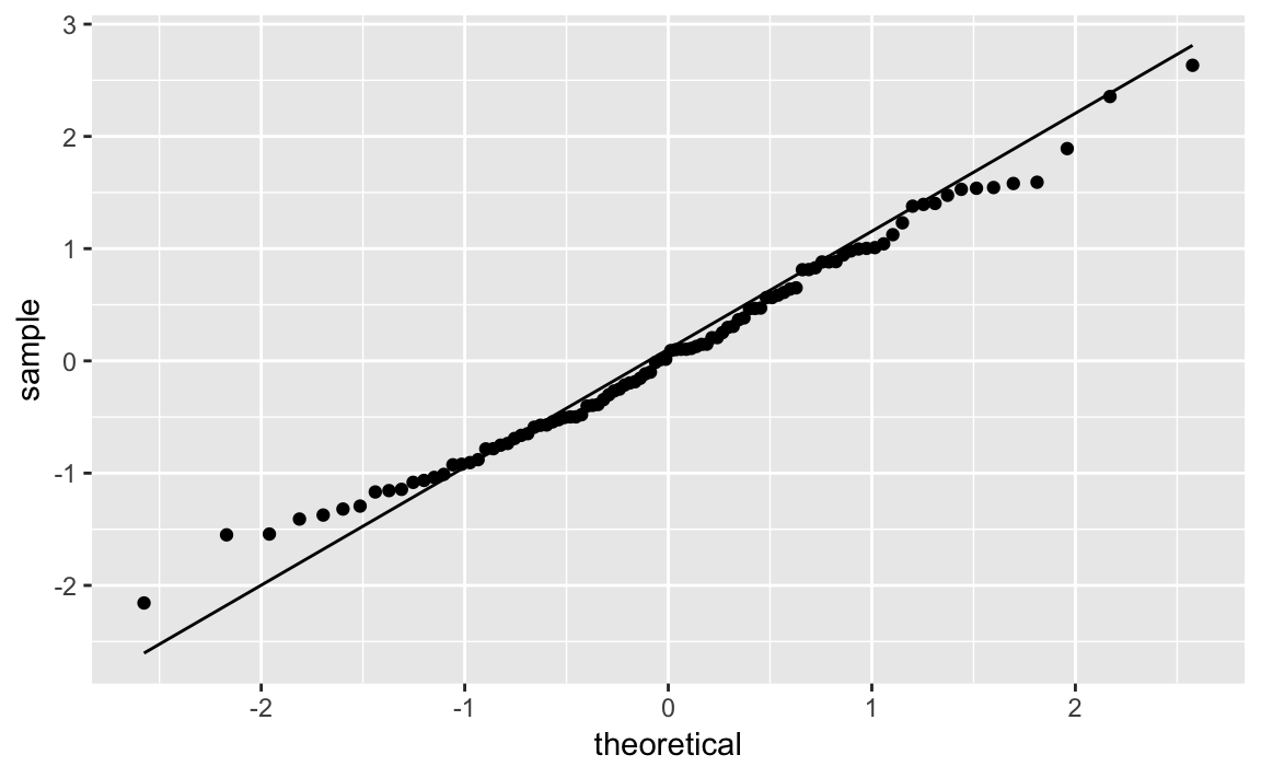
Sometimes it’s important to know if your data is normally distributed. A quantile-quantile (Q-Q) plot is a good first check.
The Cars93 dataset contains a Price column. Is it normally
distributed? This code snippet creates a Q-Q plot of Price shown in
Figure 10-34:
ggplot(Cars93,aes(sample=Price))+stat_qq()+stat_qq_line()
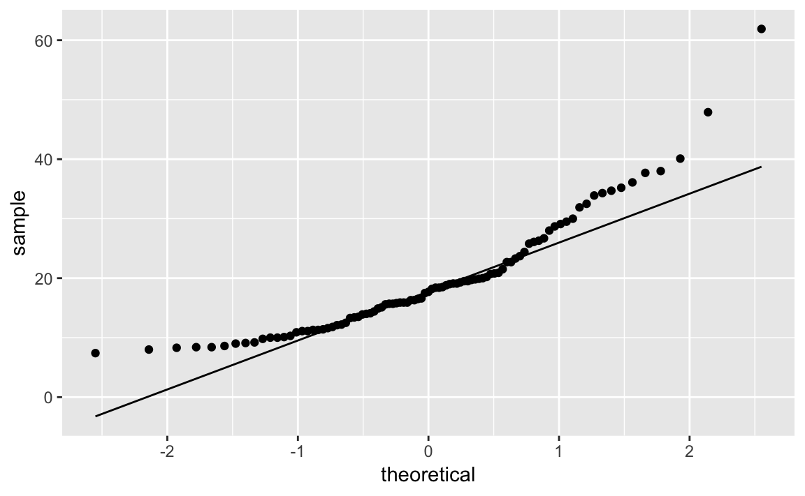
If the data had a perfect normal distribution, then the points would fall exactly on the diagonal line. Many points are close, especially in the middle section, but the points in the tails are pretty far off. Too many points are above the line, indicating a general skew to the left.
The leftward skew might be cured by a logarithmic transformation. We can plot log(Price), which yields Figure 10-35:
ggplot(Cars93,aes(sample=log(Price)))+stat_qq()+stat_qq_line()
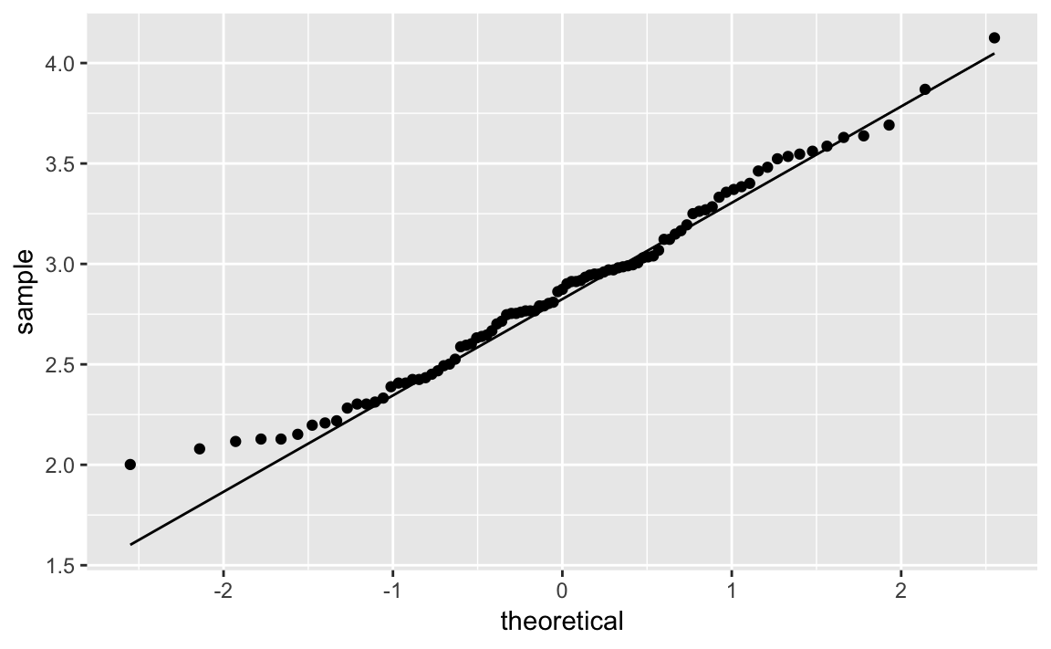
Notice that the points in the new plot are much better behaved, staying close to the line except in the extreme left tail. It appears that log(Price) is approximately Normal.
See “Creating Other Quantile-Quantile Plots” for creating Q-Q plots for other distributions. See Recipe X-X for an application of Normal Q-Q plots to diagnosing linear regression.
You want to view a quantile-quantile plot for your data, but the data is not normally distributed.
For this recipe, you must have some idea of the underlying distribution, of course. The solution is built from the following steps:
Use the ppoints function to generate a sequence of points between 0
and 1.
Transform those points into quantiles, using the quantile function for the assumed distribution.
Sort your sample data.
Plot the sorted data against the computed quantiles.
Use abline to plot the diagonal line.
This can all be done in two lines of R code. Here is an example that
assumes your data, y, has a Student’s t distribution with 5 degrees
of freedom. Recall that the quantile function for Student’s t is qt
and that its second argument is the degrees of freedom. To create draws
from
First let’s make some example data:
df_t<-data.frame(y=rt(100,5))
In order to plot the Q-Q plot we need to estimate the parameters of the
distribution we’re wanting to plot. Since this is a Student’s t
distribution, we only need to estimate one parameter, the degrees of
freedom. Of course we know the actual degrees of freedom is 5, but in
most situations we’ll need to calcuate value. So we’ll use the
MASS::fitdistr function to estimate the degrees of freedom:
est_df<-as.list(MASS::fitdistr(df_t$y,"t")$estimate)[["df"]]#> Warning in log(s): NaNs produced#> Warning in log(s): NaNs produced#> Warning in log(s): NaNs producedest_df#> [1] 19.5
As expected, that’s pretty close to what was used to generate the simulated data. So let’s pass the estimaged degrees of freedom to the Q-Q functions and create Figure 10-36:
ggplot(df_t)+aes(sample=y)+geom_qq(distribution=qt,dparams=est_df)+stat_qq_line(distribution=qt,dparams=est_df)
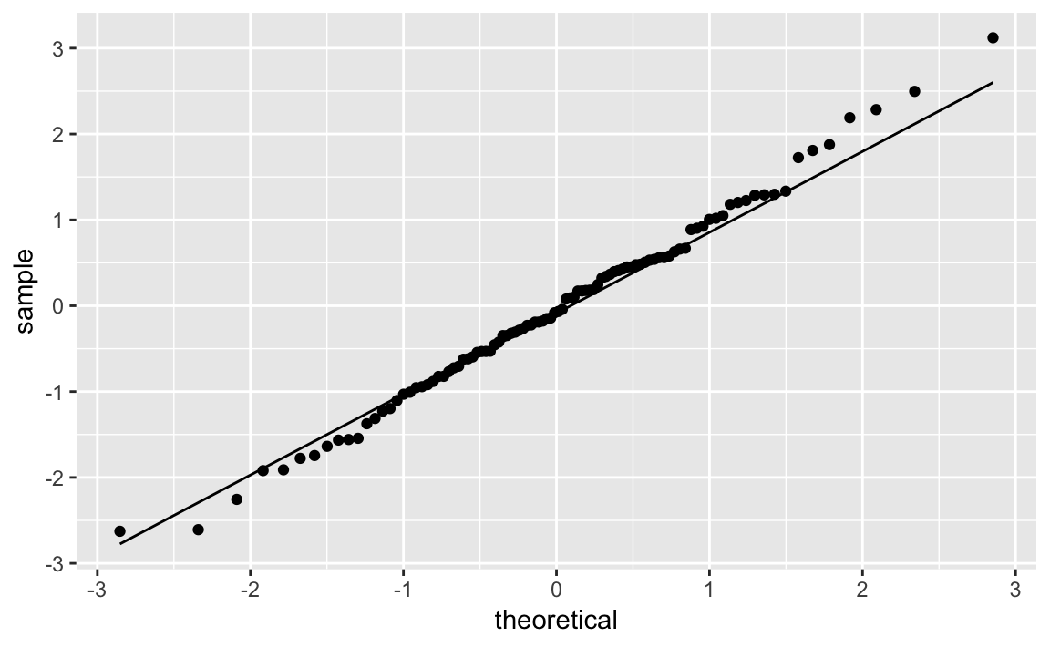
The solution looks complicated, but the gist of it is picking a
distribution, fitting the parameters, and then passing those parameters
to the Q-Q functions in ggplot.
We can illustrate this recipe by taking a random sample from an exponential distribution with a mean of 10 (or, equivalently, a rate of 1/10):
rate<-1/10n<-1000df_exp<-data.frame(y=rexp(n,rate=rate))
est_exp<-as.list(MASS::fitdistr(df_exp$y,"exponential")$estimate)[["rate"]]est_exp#> [1] 0.101
Notice that for an exponential distribution the parameter we estimate is
called rate as opposed to df which was the parameter in the t
distribution.
ggplot(df_exp)+aes(sample=y)+geom_qq(distribution=qexp,dparams=est_exp)+stat_qq_line(distribution=qexp,dparams=est_exp)

The quantile function for the exponential distribution is qexp, which
takes the rate argument. Figure 10-37 shows the resulting
Q-Q plot using a theoretical exponential distribution.
You want to plot your data in multiple colors, typically to make the plot more informative, readable, or interesting.
We can pass a color to a geom_ function in order to produced colored
output:
df<-data.frame(x=rnorm(200),y=rnorm(200))ggplot(df)+aes(x=x,y=y)+geom_point(color="blue")
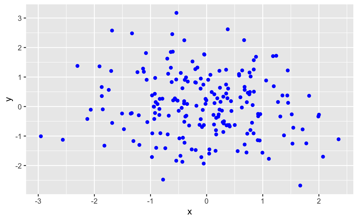
The value of color can be:
One color, in which case all data points are that color.
A vector of colors, the same length as x, in which case each value
of x is colored with its corresponding color.
A short vector, in which case the vector of colors is recycled.
The default color in ggplot is black. While it’s not very exciting,
black is high contrast and easy for most anyone to see.
However, it is much more useful (and interesting) to vary the color in a way that illuminates the data. Let’s illustrate this by plotting a graphic two ways, once in black and white and once with simple shading.
This produces the basic black-and-white graphic in Figure 10-39:
df<-data.frame(x=1:100,y=rnorm(100))ggplot(df)+aes(x,y)+geom_point()
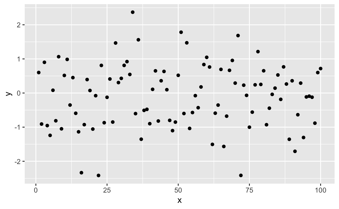
Now we can make it more interesting by creating a vector of "gray" and
"black" values, according to the sign of x and then plotting x
using those colors as shown in Figure 10-40:
shade<-if_else(df$y>=0,"black","gray")ggplot(df)+aes(x,y)+geom_point(color=shade)
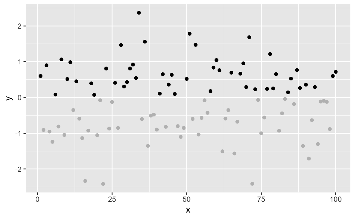
The negative values are now plotted in gray because the corresponding
element of colors is "gray".
See “Understanding the Recycling Rule” regarding the Recycling Rule. Execute colors() to see
a list of available colors, and use geom_segment in ggplot to plot
line segments in multiple colors.
You want to graph the value of a function.
The ggplot function stat_function will graph a function across a
range. In Figure 10-41 we plot a sin wave across the
range -3 to 3.
ggplot(data.frame(x=c(-3,3)))+aes(x)+stat_function(fun=sin)
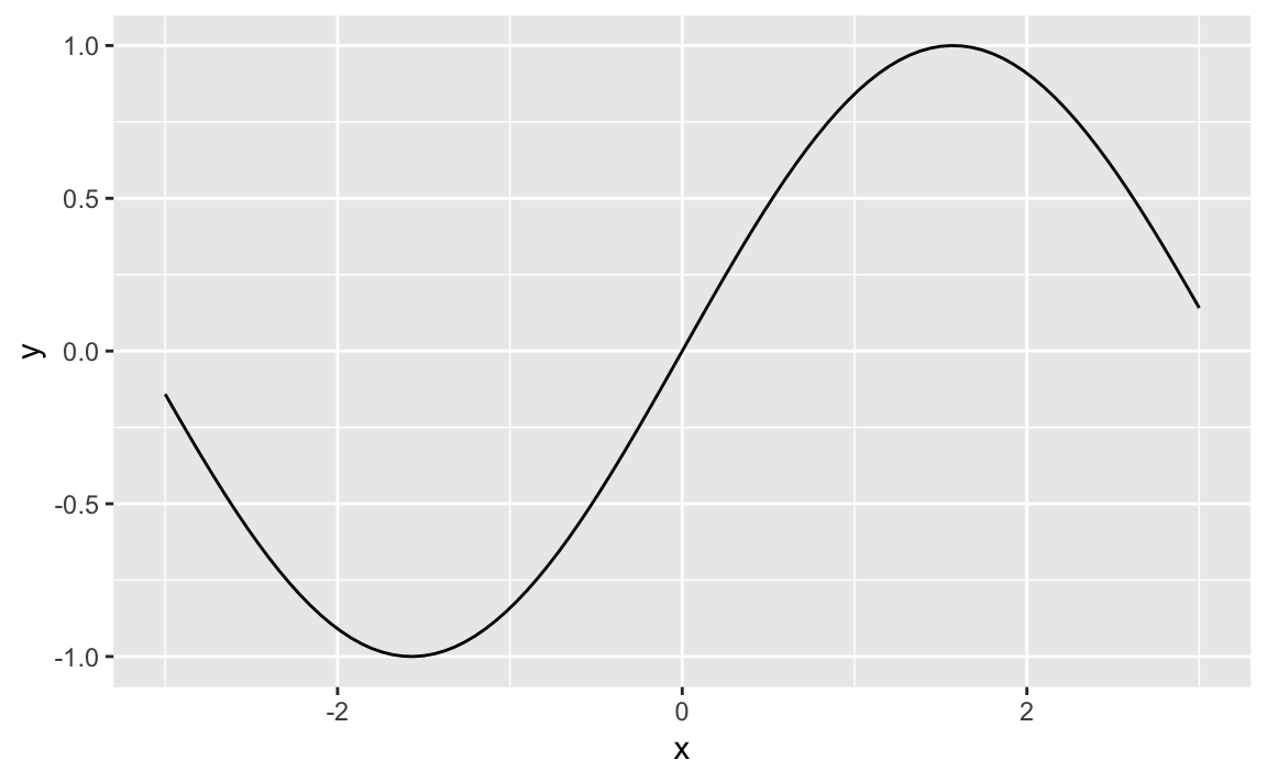
It’s pretty common to want to plot a statistical function, such as a
normal distribution across a given range. The stat_function in
ggplot allows us to do thise. We need only supply a data frame with
x value limits and stat_function will calculate the y values, and
plot the results:
ggplot(data.frame(x=c(-3.5,3.5)))+aes(x)+stat_function(fun=dnorm)+ggtitle("Std. Normal Density")
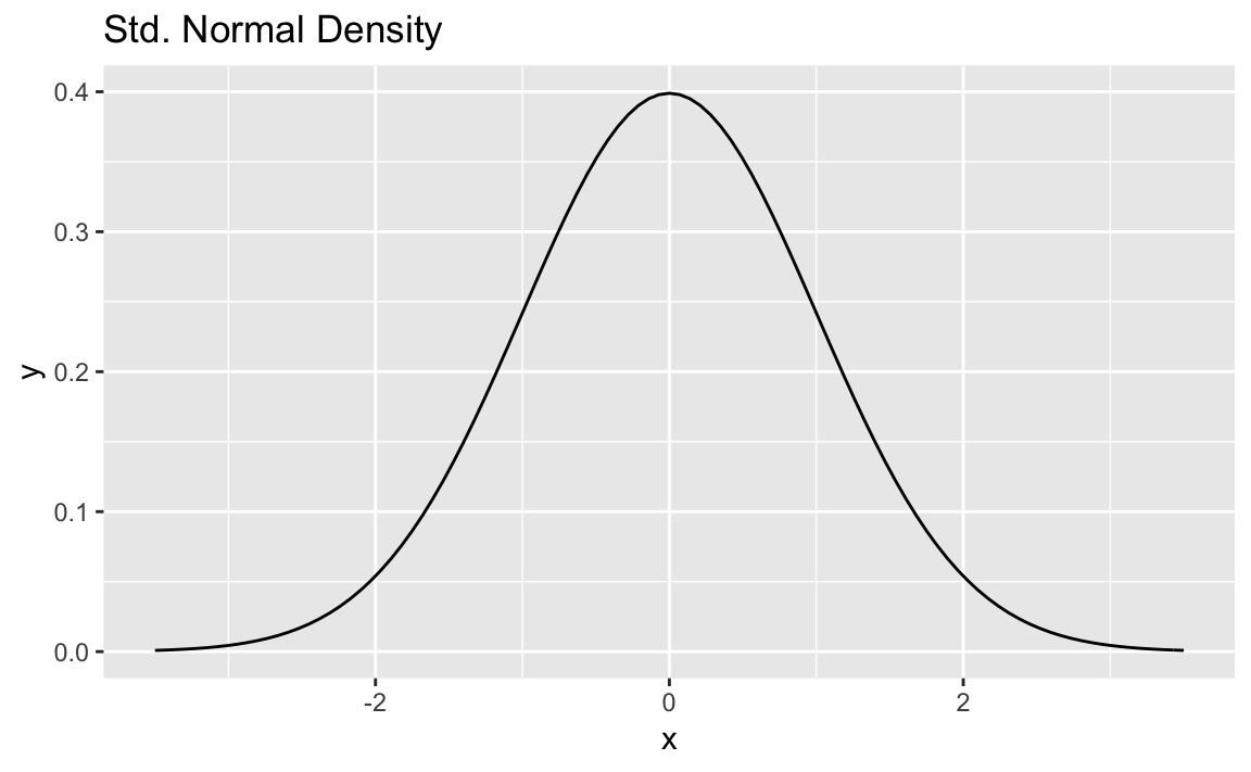
Notice in the chart above we use ggtitle to set the title. If setting
multiple text elements in a ggplot we use labs but when just adding
a title, ggtitle is more concise than
labs(title='Std. Normal Density') although they accomplish the same
thing. See ?labs for more discussion of labels with ggplot
stat_function can graph any function that takes one argument and
returns one value. Let’s create a function and then plot it. Our
function is a dampened sin wave that is a sin wave that loses amplitude
as it moves away from 0:
f<-function(x)exp(-abs(x))*sin(2*pi*x)
ggplot(data.frame(x=c(-3.5,3.5)))+aes(x)+stat_function(fun=f)+ggtitle("Dampened Sine Wave")
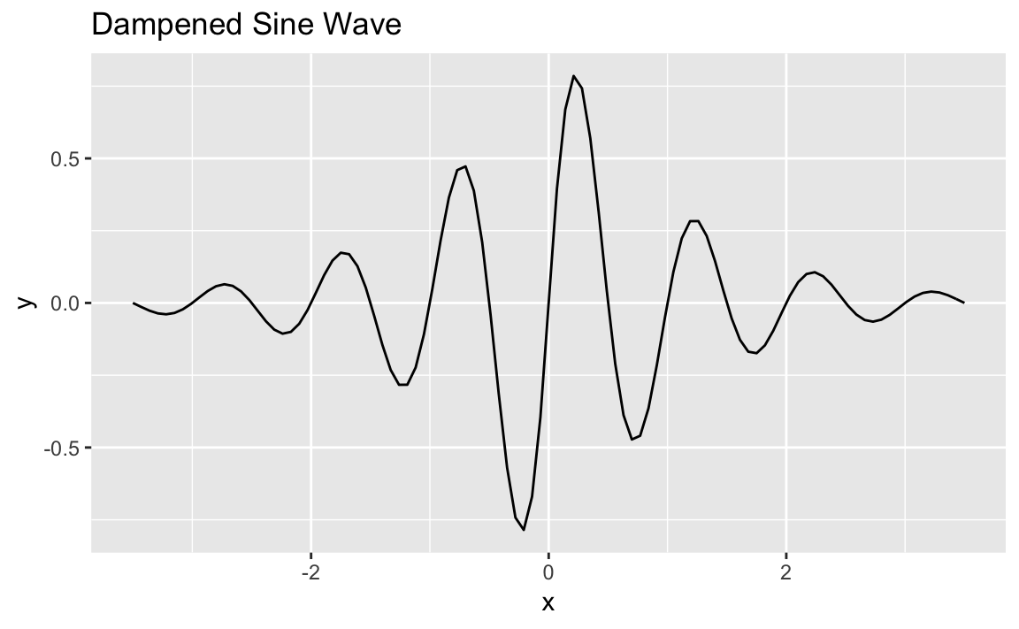
See Recipe X-X for how to define a function.
You are creating several plots, and each plot is overwriting the previous one. You want R to pause between plots so you can view each one before it’s overwritten.
There is a global graphics option called ask. Set it to TRUE, and R
will pause before each new plot. We turn on this option by passing it to
the par function which sets parameters:
par(ask=TRUE)
When you are tired of R pausing between plots, set it to FALSE:
par(ask=FALSE)
When ask is TRUE, R will print this message immediately before
starting a new plot:
Hit <Return> to see next plot:
When you are ready, hit the return or enter key and R will begin the next plot.
This is a Base R Graphics function but you can use it in ggplot if you
wrap your plot function in a print statement in order to get prompted.
Below is an example of a loop that prints a random set of points 5
times. If you run this loop in RStudio, you will be prompted between
each graphic. Notice how we wrap g inside a print call:
par(ask=TRUE)for(iin(11:15)){g<-ggplot(data.frame(x=rnorm(i),y=1:i))+aes(x,y)+geom_point()(g)}# don't forget to turn ask off after you're donepar(ask=FALSE)
If one graph is overwriting another, consider using “Displaying Several Figures on One Page” to plot multiple graphs in one frame. See Recipe X-X for more about changing graphical parameters.
JDL EDIT MARK
You want to display several plots side by side on one page.
# example dataz<-rnorm(1000)y<-runif(1000)# plot elementsp1<-ggplot()+geom_point(aes(x=1:1000,y=z))p2<-ggplot()+geom_point(aes(x=1:1000,y=y))p3<-ggplot()+geom_density(aes(z))p4<-ggplot()+geom_density(aes(y))
There are a number of ways to put ggplot graphics into a grid, but one
of the easiest to use and understand is patchwork by Thomas Lin
Pedersen. When this book was written, patchwork was not availiable on
CRAN, but can be installed using devtools:
devtools::install_github("thomasp85/patchwork")
After installing the package we can use it to plot mulitple ggplot
objects using a + between the objects then a call to plot_layout to
arrange the images into a grid as shown in Figure 10-42:
library(patchwork)p1+p2+p3+p4
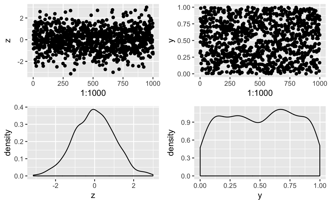
patchwork supports grouping with parenthesis and using / to put
groupings under other elements as illustrated in Figure 10-43.
p3/(p1+p2+p4)
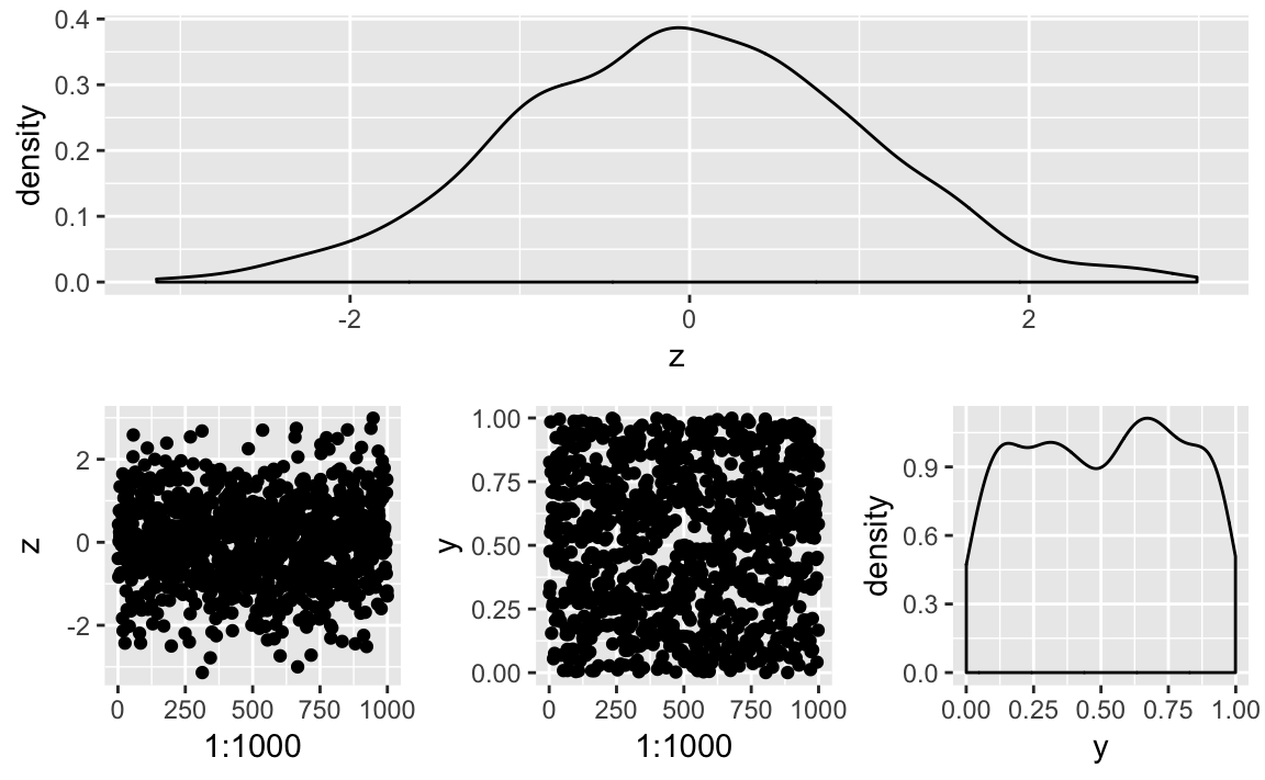
Let’s use a multifigure plot to display four different beta
distributions. Using ggplot and the patchwork package, we can create
a 2 x 2 layout effect by greating four graphics objects then print them
using the + notation from Patchwork:
library(patchwork)df<-data.frame(x=c(0,1))g1<-ggplot(df)+aes(x)+stat_function(fun=function(x)dbeta(x,2,4))+ggtitle("First")g2<-ggplot(df)+aes(x)+stat_function(fun=function(x)dbeta(x,4,1))+ggtitle("Second")g3<-ggplot(df)+aes(x)+stat_function(fun=function(x)dbeta(x,1,1))+ggtitle("Third")g4<-ggplot(df)+aes(x)+stat_function(fun=function(x)dbeta(x,.5,.5))+ggtitle("Fourth")g1+g2+g3+g4+plot_layout(ncol=2,byrow=TRUE)
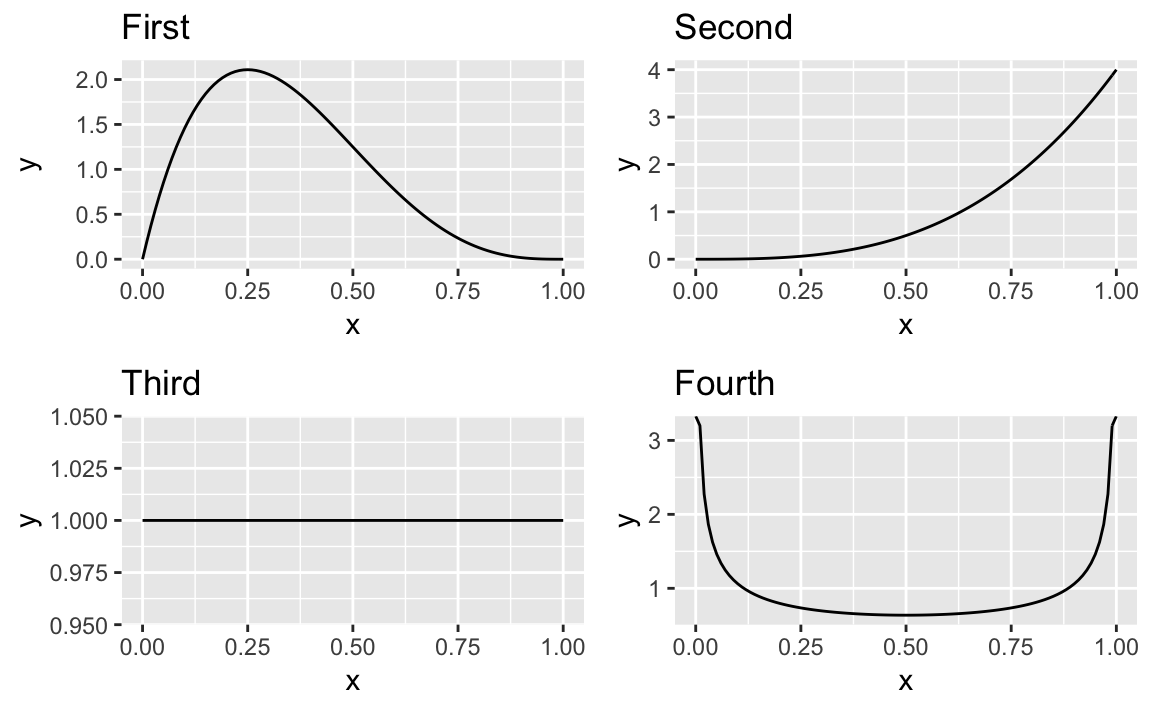
To lay the images out in columns order we could pass the byrow=FALSE
to plot_layout:
g1+g2+g3+g4+plot_layout(ncol=2,byrow=FALSE)
“Plotting a Density Function” discusses plotting of density functions as we do above.
The grid package and the lattice package contain additional tools
for multifigure layouts with Base Graphics.
You want to save your graphics in a file, such as a PNG, JPEG, or PostScript file.
With ggplot figures we can use ggsave to save a displayed image to a
file. ggsave will make some default assumptions about size and file
type for you, allowing you to only specify a filename:
ggsave("filename.jpg")
The file type is derived from the extension you use in the filename you
pass to ggsave. You can control details of size, filetype, and scale
by passing parameters to ggsave. See ?ggsave for specific details.
In RStudio, a shortcut is to click on Export in the Plots window and
then click on Save as Image, Save as PDF, or Copy to Clipboard.
The save options will prompt you for a file type and a file name before
writing the file. The Copy to Clipboard option can be handy if you are
manually copying and pasting your graphics into a presentation or word
processor.
Remember that the file will be written to your current working directory
(unless you use an absolute file path), so be certain you know which
directory is your working directory before calling savePlot.
In a non-interactive script using ggplot you can pass plot objects
directly to ggsave so they need not be displayed before saving. In the
prior recipe we created a plot object called g1. We can save it to a
file like this:
ggsave("g1.png",plot=g1,units="in",width=5,height=4)
Note that the units for height and width in ggsave are specified
with the units parameter. In this case we used in for inches, but
ggsave also supports mm and cm for the more metricly inclined.
See “Getting and Setting the Working Directory” for more about the current working directory.
In statistics, modeling is where we get down to business. Models quantify the relationships between our variables. Models let us make predictions.
A simple linear regression is the most basic model. It’s just two variables and is modeled as a linear relationship with an error term:
We are given the data for x and y. Our mission is to fit the model, which will give us the best estimates for β0 and β1 (“Performing Simple Linear Regression”).
That generalizes naturally to multiple linear regression, where we have multiple variables on the righthand side of the relationship (“Performing Multiple Linear Regression”):
Statisticians call u, v, and w the predictors and y the response. Obviously, the model is useful only if there is a fairly linear relationship between the predictors and the response, but that requirement is much less restrictive than you might think. “Regressing on Transformed Data” discusses transforming your variables into a (more) linear relationship so that you can use the well-developed machinery of linear regression.
The beauty of R is that anyone can build these linear models. The models
are built by a function, lm, which returns a model object. From the
model object, we get the coefficients (βi) and regression
statistics. It’s easy. Really!
The horror of R is that anyone can build these models. Nothing requires you to check that the model is reasonable, much less statistically significant. Before you blindly believe a model, check it. Most of the information you need is in the regression summary (“Understanding the Regression Summary”):
Check the F statistic at the bottom of the summary.
Check the coefficient’s t statistics and p-values in the summary, or check their confidence intervals (“Forming Confidence Intervals for Regression Coefficients”).
Check the R2 near the bottom of the summary.
Plot the residuals and check the regression diagnostics (Recipes and .
Check whether the diagnostics confirm that a linear model is reasonable for your data (“Diagnosing a Linear Regression”).
Analysis of variance (ANOVA) is a powerful statistical technique. First-year graduate students in statistics are taught ANOVA almost immediately because of its importance, both theoretical and practical. We are often amazed, however, at the extent to which people outside the field are unaware of its purpose and value.
Regression creates a model, and ANOVA is one method of evaluating such models. The mathematics of ANOVA are intertwined with the mathematics of regression, so statisticians usually present them together; we follow that tradition here.
ANOVA is actually a family of techniques that are connected by a common mathematical analysis. This chapter mentions several applications:
This is the simplest application of ANOVA. Suppose you have data
samples from several populations and are wondering whether the
populations have different means. One-way ANOVA answers that question.
If the populations have normal distributions, use the oneway.test
function (“Performing One-Way ANOVA”); otherwise,
use the nonparametric version, the kruskal.test function
(“Performing Robust ANOVA (Kruskal–Wallis Test)”).
When you add or delete a predictor variable from a linear regression,
you want to know whether that change did or did not improve the model.
The anova function compares two regression models and reports
whether they are significantly different (“Comparing Models by Using ANOVA”).
The anova function can also construct the ANOVA table of a linear
regression model, which includes the F statistic needed to gauge the
model’s statistical significance (“Getting Regression Statistics”). This important table is discussed in nearly
every textbook on regression.
The See Also section below contain more about the mathematics of ANOVA.
In many of the examples in this chapter, we start with creating example data using R’s pseudo random number generation capabilities. So at the beginning of each recipe you may see something like the following:
set.seed(42)x<-rnorm(100)e<-rnorm(100,mean=0,sd=5)y<-5+15*x+e
We use set.seed to set the random number generation seed so that if
you run the example code on your machine you will get the same answer.
In the above example, x is a vector of 100 draws from a standard
normal (mean=0, sd=1) distribution. Then we create a little random noise
called e from a normal distribution with mean=0 and sd=5. y is then
calculated as 5 + 15 * x + e. The idea behind creating example data
rather than using “real world” data is that with simulated “toy” data
you can change the coefficients and parameters in the example data and
see how the change impacts the resulting model. For example, you could
increase the standard deviation of e in the example data and see what
impact that has on the R^2 of your model.
There are many good texts on linear regression. One of our favorites is Applied Linear Regression Models (4th ed.) by Kutner, Nachtsheim, and Neter (McGraw-Hill/Irwin). We generally follow their terminology and conventions in this chapter.
We also like Linear Models with R by Julian Faraway (Chapman & Hall), because it illustrates regression using R and is quite readable. Earlier versions of Faraday’s work are available free on-line, too (e.g., http://cran.r-project.org/doc/contrib/Faraway-PRA.pdf).
You have two vectors, x and y, that hold paired observations: (x1, y1), (x2, y2), …, (xn, yn). You believe there is a linear relationship between x and y, and you want to create a regression model of the relationship.
The lm function performs a linear regression and reports the
coefficients:
set.seed(42)x<-rnorm(100)e<-rnorm(100,mean=0,sd=5)y<-5+15*x+elm(y~x)#>#> Call:#> lm(formula = y ~ x)#>#> Coefficients:#> (Intercept) x#> 4.56 15.14
Simple linear regression involves two variables: a predictor (or independent) variable, often called x; and a response (or dependent) variable, often called y. The regression uses the ordinary least-squares (OLS) algorithm to fit the linear model:
where β0 and β1 are the regression coefficients and the εi are the error terms.
The lm function can perform linear regression. The main argument is a
model formula, such as y ~ x. The formula has the response variable on
the left of the tilde character (~) and the predictor variable on the
right. The function estimates the regression coefficients, β0 and
β1, and reports them as the intercept and the coefficient of x,
respectively:
Coefficients:(Intercept)x4.55815.136
In this case, the regression equation is:
It is quite common for data to be captured inside a data frame, in which
case you want to perform a regression between two data frame columns.
Here, x and y are columns of a data frame dfrm:
df<-data.frame(x,y)head(df)#> x y#> 1 1.371 31.57#> 2 -0.565 1.75#> 3 0.363 5.43#> 4 0.633 23.74#> 5 0.404 7.73#> 6 -0.106 3.94
The lm function lets you specify a data frame by using the data
parameter. If you do, the function will take the variables from the data
frame and not from your workspace:
lm(y~x,data=df)# Take x and y from df#>#> Call:#> lm(formula = y ~ x, data = df)#>#> Coefficients:#> (Intercept) x#> 4.56 15.14
You have several predictor variables (e.g., u, v, and w) and a response variable y. You believe there is a linear relationship between the predictors and the response, and you want to perform a linear regression on the data.
Use the lm function. Specify the multiple predictors on the righthand
side of the formula, separated by plus signs (+):
lm(y~u+v+w)
Multiple linear regression is the obvious generalization of simple linear regression. It allows multiple predictor variables instead of one predictor variable and still uses OLS to compute the coefficients of a linear equation. The three-variable regression just given corresponds to this linear model:
R uses the lm function for both simple and multiple linear regression.
You simply add more variables to the righthand side of the model
formula. The output then shows the coefficients of the fitted model:
set.seed(42)u<-rnorm(100)v<-rnorm(100,mean=3,sd=2)w<-rnorm(100,mean=-3,sd=1)e<-rnorm(100,mean=0,sd=3)y<-5+4*u+3*v+2*w+elm(y~u+v+w)#>#> Call:#> lm(formula = y ~ u + v + w)#>#> Coefficients:#> (Intercept) u v w#> 4.77 4.17 3.01 1.91
The data parameter of lm is especially valuable when the number of
variables increases, since it’s much easier to keep your data in one
data frame than in many separate variables. Suppose your data is
captured in a data frame, such as the df variable shown here:
df<-data.frame(y,u,v,w)head(df)#> y u v w#> 1 16.67 1.371 5.402 -5.00#> 2 14.96 -0.565 5.090 -2.67#> 3 5.89 0.363 0.994 -1.83#> 4 27.95 0.633 6.697 -0.94#> 5 2.42 0.404 1.666 -4.38#> 6 5.73 -0.106 3.211 -4.15
When we supply df to the data parameter of lm, R looks for the
regression variables in the columns of the data frame:
lm(y~u+v+w,data=df)#>#> Call:#> lm(formula = y ~ u + v + w, data = df)#>#> Coefficients:#> (Intercept) u v w#> 4.77 4.17 3.01 1.91
See “Performing Simple Linear Regression” for simple linear regression.
You want the critical statistics and information regarding your regression, such as R2, the F statistic, confidence intervals for the coefficients, residuals, the ANOVA table, and so forth.
Save the regression model in a variable, say m:
m<-lm(y~u+v+w)
Then use functions to extract regression statistics and information from the model:
anova(m)ANOVA table
coefficients(m)Model coefficients
coef(m)Same as coefficients(m)
confint(m)Confidence intervals for the regression coefficients
deviance(m)Residual sum of squares
effects(m)Vector of orthogonal effects
fitted(m)Vector of fitted y values
residuals(m)Model residuals
resid(m)Same as residuals(m)
summary(m)Key statistics, such as R2, the F statistic, and the residual standard error (σ)
vcov(m)Variance–covariance matrix of the main parameters
When we started using R, the documentation said use the lm function to
perform linear regression. So we did something like this, getting the
output shown in “Performing Multiple Linear Regression”:
lm(y~u+v+w)#>#> Call:#> lm(formula = y ~ u + v + w)#>#> Coefficients:#> (Intercept) u v w#> 4.77 4.17 3.01 1.91
How disappointing! The output was nothing compared to other statistics packages such as SAS. Where is R2? Where are the confidence intervals for the coefficients? Where is the F statistic, its p-value, and the ANOVA table?
Of course, all that information is available—you just have to ask for it. Other statistics systems dump everything and let you wade through it. R is more minimalist. It prints a bare-bones output and lets you request what more you want.
The lm function returns a model object that you can assign to a
variable:
m<-lm(y~u+v+w)
From the model object, you can extract important information using
specialized functions. The most important function is summary:
summary(m)#>#> Call:#> lm(formula = y ~ u + v + w)#>#> Residuals:#> Min 1Q Median 3Q Max#> -5.383 -1.760 -0.312 1.856 6.984#>#> Coefficients:#> Estimate Std. Error t value Pr(>|t|)#> (Intercept) 4.770 0.969 4.92 3.5e-06 ***#> u 4.173 0.260 16.07 < 2e-16 ***#> v 3.013 0.148 20.31 < 2e-16 ***#> w 1.905 0.266 7.15 1.7e-10 ***#> ---#> Signif. codes: 0 '***' 0.001 '**' 0.01 '*' 0.05 '.' 0.1 ' ' 1#>#> Residual standard error: 2.66 on 96 degrees of freedom#> Multiple R-squared: 0.885, Adjusted R-squared: 0.882#> F-statistic: 247 on 3 and 96 DF, p-value: <2e-16
The summary shows the estimated coefficients. It shows the critical statistics, such as R2 and the F statistic. It shows an estimate of σ, the standard error of the residuals. The summary is so important that there is an entire recipe devoted to understanding it (“Understanding the Regression Summary”).
There are specialized extractor functions for other important information:
coef(m)#> (Intercept) u v w#> 4.77 4.17 3.01 1.91
confint(m)#> 2.5 % 97.5 %#> (Intercept) 2.85 6.69#> u 3.66 4.69#> v 2.72 3.31#> w 1.38 2.43
resid(m)#> 1 2 3 4 5 6 7 8 9#> -0.5675 2.2880 0.0972 2.1474 -0.7169 -0.3617 1.0350 2.8040 -4.2496#> 10 11 12 13 14 15 16 17 18#> -0.2048 -0.6467 -2.5772 -2.9339 -1.9330 1.7800 -1.4400 -2.3989 0.9245#> 19 20 21 22 23 24 25 26 27#> -3.3663 2.6890 -1.4190 0.7871 0.0355 -0.3806 5.0459 -2.5011 3.4516#> 28 29 30 31 32 33 34 35 36#> 0.3371 -2.7099 -0.0761 2.0261 -1.3902 -2.7041 0.3953 2.7201 -0.0254#> 37 38 39 40 41 42 43 44 45#> -3.9887 -3.9011 -1.9458 -1.7701 -0.2614 2.0977 -1.3986 -3.1910 1.8439#> 46 47 48 49 50 51 52 53 54#> 0.8218 3.6273 -5.3832 0.2905 3.7878 1.9194 -2.4106 1.6855 -2.7964#> 55 56 57 58 59 60 61 62 63#> -1.3348 3.3549 -1.1525 2.4012 -0.5320 -4.9434 -2.4899 -3.2718 -1.6161#> 64 65 66 67 68 69 70 71 72#> -1.5119 -0.4493 -0.9869 5.6273 -4.4626 -1.7568 0.8099 5.0320 0.1689#> 73 74 75 76 77 78 79 80 81#> 3.5761 -4.8668 4.2781 -2.1386 -0.9739 -3.6380 0.5788 5.5664 6.9840#> 82 83 84 85 86 87 88 89 90#> -3.5119 1.2842 4.1445 -0.4630 -0.7867 -0.7565 1.6384 3.7578 1.8942#> 91 92 93 94 95 96 97 98 99#> 0.5542 -0.8662 1.2041 -1.7401 -0.7261 3.2701 1.4012 0.9476 -0.9140#> 100#> 2.4278
deviance(m)#> [1] 679
anova(m)#> Analysis of Variance Table#>#> Response: y#> Df Sum Sq Mean Sq F value Pr(>F)#> u 1 1776 1776 251.0 < 2e-16 ***#> v 1 3097 3097 437.7 < 2e-16 ***#> w 1 362 362 51.1 1.7e-10 ***#> Residuals 96 679 7#> ---#> Signif. codes: 0 '***' 0.001 '**' 0.01 '*' 0.05 '.' 0.1 ' ' 1
If you find it annoying to save the model in a variable, you are welcome to use one-liners such as this:
summary(lm(y~u+v+w))
Or you can use Magritr pipes:
lm(y~u+v+w)%>%summary
See “Understanding the Regression Summary”. See “Identifying Influential Observations” for regression statistics specific to model diagnostics.
You created a linear regression model, m. However, you are confused by
the output from summary(m).
The model summary is important because it links you to the most critical regression statistics. Here is the model summary from “Getting Regression Statistics”:
summary(m)#>#> Call:#> lm(formula = y ~ u + v + w)#>#> Residuals:#> Min 1Q Median 3Q Max#> -5.383 -1.760 -0.312 1.856 6.984#>#> Coefficients:#> Estimate Std. Error t value Pr(>|t|)#> (Intercept) 4.770 0.969 4.92 3.5e-06 ***#> u 4.173 0.260 16.07 < 2e-16 ***#> v 3.013 0.148 20.31 < 2e-16 ***#> w 1.905 0.266 7.15 1.7e-10 ***#> ---#> Signif. codes: 0 '***' 0.001 '**' 0.01 '*' 0.05 '.' 0.1 ' ' 1#>#> Residual standard error: 2.66 on 96 degrees of freedom#> Multiple R-squared: 0.885, Adjusted R-squared: 0.882#> F-statistic: 247 on 3 and 96 DF, p-value: <2e-16
Let’s dissect this summary by section. We’ll read it from top to bottom—even though the most important statistic, the F statistic, appears at the end:
summary(m)$call
This shows how lm was called when it created the model, which is
important for putting this summary into the proper context.
# Residuals:
# Min 1Q Median 3Q Max
# -5.3832 -1.7601 -0.3115 1.8565 6.9840
Ideally, the regression residuals would have a perfect, normal distribution. These statistics help you identify possible deviations from normality. The OLS algorithm is mathematically guaranteed to produce residuals with a mean of zero.[‸1] Hence the sign of the median indicates the skew’s direction, and the magnitude of the median indicates the extent. In this case the median is negative, which suggests some skew to the left.
If the residuals have a nice, bell-shaped distribution, then the first quartile (1Q) and third quartile (3Q) should have about the same magnitude. In this example, the larger magnitude of 3Q versus 1Q (1.3730 versus 0.9472) indicates a slight skew to the right in our data, although the negative median makes the situation less clear-cut.
The Min and Max residuals offer a quick way to detect extreme outliers in the data, since extreme outliers (in the response variable) produce large residuals.
summary(m)$coefficients#> Estimate Std. Error t value Pr(>|t|)#> (Intercept) 4.77 0.969 4.92 3.55e-06#> u 4.17 0.260 16.07 5.76e-29#> v 3.01 0.148 20.31 1.58e-36#> w 1.91 0.266 7.15 1.71e-10
The column labeled Estimate contains the estimated regression
coefficients as calculated by ordinary least squares.
Theoretically, if a variable’s coefficient is zero then the variable
is worthless; it adds nothing to the model. Yet the coefficients
shown here are only estimates, and they will never be exactly zero.
We therefore ask: Statistically speaking, how likely is it that the
true coefficient is zero? That is the purpose of the t statistics
and the p-values, which in the summary are labeled (respectively)
t value and Pr(>|t|).
The p-value is a probability. It gauges the likelihood that the coefficient is not significant, so smaller is better. Big is bad because it indicates a high likelihood of insignificance. In this example, the p-value for the u coefficient is a mere 0.00106, so u is likely significant. The p-value for w, however, is 0.05744; this is just over our conventional limit of 0.05, which suggests that w is likely insignificant.[^2] Variables with large p-values are candidates for elimination.
A handy feature is that R flags the significant variables for
quick identification. Do you notice the extreme righthand column
containing double asterisks (**), a single asterisk (*), and a
period(.)? That column highlights the significant variables. The
line labeled "Signif. codes" at the bottom gives a cryptic guide
to the flags’ meanings:
+
--------- ----------------------------------
*** p-value between 0 and 0.001
** p-value between 0.001 and 0.01
* p-value between 0.01 and 0.05
. p-value between 0.05 and 0.1
(blank) p-value between 0.1 and 1.0
--------- ----------------------------------
+
The column labeled Std. Error is the standard error of the
estimated coefficient. The column labeled t value is the t
statistic from which the p-value was calculated.
Residual standard error:: + [source, r]
# Residual standard error: 2.66 on 96 degrees of freedom
+ ------------------------------------------------------------------- This reports the standard error of the residuals (*σ*)—that is, the sample standard deviation of *ε*. ------------------------------------------------------------------- _R_^2^ (coefficient of determination):: + [source, r]
# Multiple R-squared: 0.8851, Adjusted R-squared: 0.8815
+ ------------------------------------------------------------------- *R*^2^ is a measure of the model’s quality. Bigger is better. Mathematically, it is the fraction of the variance of *y* that is explained by the regression model. The remaining variance is not explained by the model, so it must be due to other factors (i.e., unknown variables or sampling variability). In this case, the model explains 0.4981 (49.81%) of the variance of *y*, and the remaining 0.5019 (50.19%) is unexplained. That being said, we strongly suggest using the adjusted rather than the basic *R*^2^. The adjusted value accounts for the number of variables in your model and so is a more realistic assessment of its effectiveness. In this case, then, we would use 0.8815, not 0.8851s ------------------------------------------------------------------- _F_ statistic:: + [source, r]
# F-statistic: 246.6 on 3 and 96 DF, p-value: < 2.2e-16
+ -------------------------------------------------------------------- The *F* statistic tells you whether the model is significant or insignificant. The model is significant if any of the coefficients are nonzero (i.e., if *β*~*i*~ ≠ 0 for some *i*). It is insignificant if all coefficients are zero (*β*~1~ = *β*~2~ = … = *β*~*n*~ = 0). Conventionally, a *p*-value of less than 0.05 indicates that the model is likely significant (one or more *β*~*i*~ are nonzero) whereas values exceeding 0.05 indicate that the model is likely not significant. Here, the probability is only 0.000391 that our model is insignificant. That’s good. Most people look at the *R*^2^ statistic first. The statistician wisely starts with the *F* statistic, for if the model is not significant then nothing else matters. -------------------------------------------------------------------- [[see_also-id240]] ==== See Also See <<recipe-id231>> for more on extracting statistics and information from the model object. [[recipe-id205]] === Performing Linear Regression Without an Intercept [[problem-id205]] ==== Problem You want to perform a linear regression, but you want to force the intercept to be zero. [[solution-id205]] ==== Solution Add "`+` `0`" to the righthand side of your regression formula. That will force `lm` to fit the model with a zero intercept: [source, r]
lm(y ~ x + 0)
The corresponding regression equation is: ++++ <ul class="simplelist"> <li><em>y</em><sub><em>i</em></sub> = <em>βx</em><sub><em>i</em></sub> + <em>ε</em><sub><em>i</em></sub></li> </ul> ++++ [[discussion-id205]] ==== Discussion Linear regression ordinarily includes an intercept term, so that is the default in R. In rare cases, however, you may want to fit the data while assuming that the intercept is zero. In this you make a modeling assumption: when _x_ is zero, _y_ should be zero. When you force a zero intercept, the `lm` output includes a coefficient for _x_ but no intercept for _y_, as shown here: [source, r]
lm(y x + 0) #> #> Call: #> lm(formula = y x + 0) #> #> Coefficients: #> x #> 4.3
We strongly suggest you check that modeling assumption before proceeding. Perform a regression with an intercept; then see if the intercept could plausibly be zero. Check the intercept’s confidence interval. In this example, the confidence interval is (6.26, 8.84): [source, r]
confint(lm(y ~ x)) #> 2.5 % 97.5 % #> (Intercept) 6.26 8.84 #> x 2.82 5.31
Because the confidence interval does not contain zero, it is NOT statistically plausible that the intercept could be zero. So in this case, it is not reasonable to rerun the regression while forcing a zero intercept. [[title-highcor]] === Regressing Only Variables that Highly Correlate with your Dependent Variable [[problem-highcor]] ==== Problem You have a data frame with many variables and you want to build a multiple linear regression using only the variables that are highly correlated to your response (dependent) variable. [[solution-highcor]] ==== Solution If `df` is our data frame containing both our response (dependent) and all our predictor (independent) variables and `dep_var` is our response variable, we can figure out our best predictors and then use them in a linear regression. If we want the top 4 predictor variables, we can use this recipe: [source, r]
best_pred ← df %>% select(-dep_var) %>% map_dbl(cor, y = df$dep_var) %>% sort(decreasing = TRUE) %>% .[1:4] %>% names %>% df[.]
mod ← lm(df$dep_var ~ as.matrix(best_pred))
This recipe is a combination of many differnt pieces of logic used elsewhere in this book. We will describe each step here then walk through it in the discussion using some example data. First we drop the response variable out of our pipe chain so that we have only our predictor variables in our data flow: [source, r]
df %>% select(-dep_var)
Then we use `map_dbl` from `purrr` to perform a pairwise correlation on each column relative to the response variable. [source, r]
map_dbl(cor, y = df$dep_var) %>%
We then take the resulting correlations and sort them in decreasing order: [source, r]
sort(decreasing = TRUE) %>%
We want only the top 4 correlated variables so we select the top 4 records in the resulting vector: [source, r]
.[1:4] %>%
And we don't need the correlation values, only the names of the rows which are the variable names from our original data frame `df`: [source, r]
names %>%
Then we can pass those names into our subsetting brackets to select only the columns with names matching the ones we want: [source, r]
Our pipe chain assigns the resulting data frame into best_pred. We can
then use best_pred as the predictor variables in our regression and we
can use df$dep_var as the response
mod<-lm(df$dep_var~as.matrix(best_pred))
We can combine the mapping functions discussed in recpie @ref(recipe-id157): “Applying a Function to Every Column” and create a recipe to remove low-correlation variables from a set of predictors and use the high correlation predictors in a regression.
We have an example data frame that contains 6 predictor variables named
pred1 through pred6. The response variable is named resp. Let’s
walk that data frame through our logic and see how it works.
Loading the data and dropping the resp variable is pretty straight
forward. So let’s look at the result of mapping the cor function:
# loads the pred data frameload("./data/pred.rdata")pred%>%select(-resp)%>%map_dbl(cor,y=pred$resp)#> pred1 pred2 pred3 pred4 pred5 pred6#> 0.573 0.279 0.753 0.799 0.322 0.607
The output is a named vector of values where the names are the variable
names and the values are the pairwise correlations between each
predictor variable and resp, the response variable.
If we sort this vector, we get the correlations in decreasing order:
pred%>%select(-resp)%>%map_dbl(cor,y=pred$resp)%>%sort(decreasing=TRUE)#> pred4 pred3 pred6 pred1 pred5 pred2#> 0.799 0.753 0.607 0.573 0.322 0.279
Using subsetting allows us to select the top 4 records. The . operator
is a special operator that tells the pipe where to put the result of the
prior step.
pred%>%select(-resp)%>%map_dbl(cor,y=pred$resp)%>%sort(decreasing=TRUE)%>%.[1:4]#> pred4 pred3 pred6 pred1#> 0.799 0.753 0.607 0.573
We then use the names function to extract the names from our vector.
The names are the names of the columns we ultimatly want to use as our
independent variables:
pred%>%select(-resp)%>%map_dbl(cor,y=pred$resp)%>%sort(decreasing=TRUE)%>%.[1:4]%>%names#> [1] "pred4" "pred3" "pred6" "pred1"
When we pass the vecotr of names into pred[.] the names are used to
select columns from the pred data frame. We then use head to select
only the top 6 rows for easier illustration:
pred%>%select(-resp)%>%map_dbl(cor,y=pred$resp)%>%sort(decreasing=TRUE)%>%.[1:4]%>%names%>%pred[.]%>%head#> pred4 pred3 pred6 pred1#> 1 7.252 1.5127 0.560 0.206#> 2 2.076 0.2579 -0.124 -0.361#> 3 -0.649 0.0884 0.657 0.758#> 4 1.365 -0.1209 0.122 -0.727#> 5 -5.444 -1.1943 -0.391 -1.368#> 6 2.554 0.6120 1.273 0.433
Now let’s bring it all together and pass the resulting data into the regression:
best_pred<-pred%>%select(-resp)%>%map_dbl(cor,y=pred$resp)%>%sort(decreasing=TRUE)%>%.[1:4]%>%names%>%pred[.]mod<-lm(pred$resp~as.matrix(best_pred))summary(mod)#>#> Call:#> lm(formula = pred$resp ~ as.matrix(best_pred))#>#> Residuals:#> Min 1Q Median 3Q Max#> -1.485 -0.619 0.189 0.562 1.398#>#> Coefficients:#> Estimate Std. Error t value Pr(>|t|)#> (Intercept) 1.117 0.340 3.28 0.0051 **#> as.matrix(best_pred)pred4 0.523 0.207 2.53 0.0231 *#> as.matrix(best_pred)pred3 -0.693 0.870 -0.80 0.4382#> as.matrix(best_pred)pred6 1.160 0.682 1.70 0.1095#> as.matrix(best_pred)pred1 0.343 0.359 0.95 0.3549#> ---#> Signif. codes: 0 '***' 0.001 '**' 0.01 '*' 0.05 '.' 0.1 ' ' 1#>#> Residual standard error: 0.927 on 15 degrees of freedom#> Multiple R-squared: 0.838, Adjusted R-squared: 0.795#> F-statistic: 19.4 on 4 and 15 DF, p-value: 8.59e-06
You want to include an interaction term in your regression.
The R syntax for regression formulas lets you specify interaction terms.
The interaction of two variables, u and v, is indicated by
separating their names with an asterisk (*):
lm(y~u*v)
This corresponds to the model yi = β0 + β1ui
β2vi + β3uivi + εi, which includes the
first-order interaction term β3uivi.
In regression, an interaction occurs when the product of two predictor variables is also a significant predictor (i.e., in addition to the predictor variables themselves). Suppose we have two predictors, u and v, and want to include their interaction in the regression. This is expressed by the following equation:
Here the product term, β3uivi, is called the interaction term. The R formula for that equation is:
y~u*v
When you write y ~ u*v, R automatically includes u, v, and
their product in the model. This is for a good reason. If a model
includes an interaction term, such as β3uivi, then
regression theory tells us the model should also contain the constituent
variables ui and vi.
Likewise, if you have three predictors (u, v, and w) and want to include all their interactions, separate them by asterisks:
y~u*v*w
This corresponds to the regression equation:
Now we have all the first-order interactions and a second-order interaction (β7uiviwi).
Sometimes, however, you may not want every possible interaction. You can
explicitly specify a single product by using the colon operator (:).
For example, u:v:w denotes the product term βuiviwi
but without all possible interactions. So the R formula:
y~u+v+w+u:v:w
corresponds to the regression equation:
It might seem odd that colon (:) means pure multiplication while
asterisk (*) means both multiplication and inclusion of constituent
terms. Again, this is because we normally incorporate the constituents
when we include their interaction, so making that the default for
asterisk makes sense.
There is some additional syntax for easily specifying many interactions:
(u + v + ... + w)^2
: Include all variables (u, v, …, w) and all their first-order interactions.
(u + v + ... + w)^3
: Include all variables, all their first-order interactions, and all their second-order interactions.
(u + v + ... + w)^4
: And so forth.
Both the asterisk (*) and the colon (:) follow a “distributive law”,
so the following notations are also allowed:
x*(u + v + ... + w)
: Same as x*u + x*v + ... + x*w (which is the same
as x + u + v + ... + w + x:u + x:v + ... + x:w).
x:(u + v + ... + w)
: Same as x:u + x:v + ... + x:w.
All this syntax gives you some flexibility in writing your formula. For example, these three formulas are equivalent:
y~u*vy~u+v+u:vy~(u+v)^2
They all define the same regression equation, yi = β0
β1ui + β2vi + β3uivi + εi .
The full syntax for formulas is richer than described here. See R in a Nutshell (O’Reilly) or the R Language Definition for more details.
You are creating a new regression model or improving an existing model. You have the luxury of many regression variables, and you want to select the best subset of those variables.
The step function can perform stepwise regression, either forward or
backward. Backward stepwise regression starts with many variables and
removes the underperformers:
full.model<-lm(y~x1+x2+x3+x4)reduced.model<-step(full.model,direction="backward")
Forward stepwise regression starts with a few variables and adds new ones to improve the model until it cannot be improved further:
min.model<-lm(y~1)fwd.model<-step(min.model,direction="forward",scope=(~x1+x2+x3+x4))
When you have many predictors, it can be quite difficult to choose the best subset. Adding and removing individual variables affects the overall mix, so the search for “the best” can become tedious.
The step function automates that search. Backward stepwise regression
is the easiest approach. Start with a model that includes all the
predictors. We call that the full model. The model summary, shown here,
indicates that not all predictors are statistically significant:
# example dataset.seed(4)n<-150x1<-rnorm(n)x2<-rnorm(n,1,2)x3<-rnorm(n,3,1)x4<-rnorm(n,-2,2)e<-rnorm(n,0,3)y<-4+x1+5*x3+e# build the modelfull.model<-lm(y~x1+x2+x3+x4)summary(full.model)#>#> Call:#> lm(formula = y ~ x1 + x2 + x3 + x4)#>#> Residuals:#> Min 1Q Median 3Q Max#> -8.032 -1.774 0.158 2.032 6.626#>#> Coefficients:#> Estimate Std. Error t value Pr(>|t|)#> (Intercept) 3.40224 0.80767 4.21 4.4e-05 ***#> x1 0.53937 0.25935 2.08 0.039 *#> x2 0.16831 0.12291 1.37 0.173#> x3 5.17410 0.23983 21.57 < 2e-16 ***#> x4 -0.00982 0.12954 -0.08 0.940#> ---#> Signif. codes: 0 '***' 0.001 '**' 0.01 '*' 0.05 '.' 0.1 ' ' 1#>#> Residual standard error: 2.92 on 145 degrees of freedom#> Multiple R-squared: 0.77, Adjusted R-squared: 0.763#> F-statistic: 121 on 4 and 145 DF, p-value: <2e-16
We want to eliminate the insignificant variables, so we use step to
incrementally eliminate the underperformers. The result is called the
reduced model:
reduced.model<-step(full.model,direction="backward")#> Start: AIC=327#> y ~ x1 + x2 + x3 + x4#>#> Df Sum of Sq RSS AIC#> - x4 1 0 1240 325#> - x2 1 16 1256 327#> <none> 1240 327#> - x1 1 37 1277 329#> - x3 1 3979 5219 540#>#> Step: AIC=325#> y ~ x1 + x2 + x3#>#> Df Sum of Sq RSS AIC#> - x2 1 16 1256 325#> <none> 1240 325#> - x1 1 37 1277 327#> - x3 1 3988 5228 539#>#> Step: AIC=325#> y ~ x1 + x3#>#> Df Sum of Sq RSS AIC#> <none> 1256 325#> - x1 1 44 1300 328#> - x3 1 3974 5230 537
The output from step shows the sequence of models that it explored. In
this case, step removed x2 and x4 and left only x1 and x3 in
the final (reduced) model. The summary of the reduced model shows that
it contains only significant predictors:
summary(reduced.model)#>#> Call:#> lm(formula = y ~ x1 + x3)#>#> Residuals:#> Min 1Q Median 3Q Max#> -8.148 -1.850 -0.055 2.026 6.550#>#> Coefficients:#> Estimate Std. Error t value Pr(>|t|)#> (Intercept) 3.648 0.751 4.86 3e-06 ***#> x1 0.582 0.255 2.28 0.024 *#> x3 5.147 0.239 21.57 <2e-16 ***#> ---#> Signif. codes: 0 '***' 0.001 '**' 0.01 '*' 0.05 '.' 0.1 ' ' 1#>#> Residual standard error: 2.92 on 147 degrees of freedom#> Multiple R-squared: 0.767, Adjusted R-squared: 0.763#> F-statistic: 241 on 2 and 147 DF, p-value: <2e-16
Backward stepwise regression is easy, but sometimes it’s not feasible to start with “everything” because you have too many candidate variables. In that case use forward stepwise regression, which will start with nothing and incrementally add variables that improve the regression. It stops when no further improvement is possible.
A model that “starts with nothing” may look odd at first:
min.model<-lm(y~1)
This is a model with a response variable (y) but no predictor variables. (All the fitted values for y are simply the mean of y, which is what you would guess if no predictors were available.)
We must tell step which candidate variables are available for
inclusion in the model. That is the purpose of the scope argument. The
scope is a formula with nothing on the lefthand side of the tilde
(~) and candidate variables on the righthand side:
fwd.model<-step(min.model,direction="forward",scope=(~x1+x2+x3+x4),trace=0)
Here we see that x1, x2, x3, and x4 are all candidates for
inclusion. (We also included trace=0 to inhibit the voluminous output
from step.) The resulting model has two significant predictors and no
insignificant predictors:
summary(fwd.model)#>#> Call:#> lm(formula = y ~ x3 + x1)#>#> Residuals:#> Min 1Q Median 3Q Max#> -8.148 -1.850 -0.055 2.026 6.550#>#> Coefficients:#> Estimate Std. Error t value Pr(>|t|)#> (Intercept) 3.648 0.751 4.86 3e-06 ***#> x3 5.147 0.239 21.57 <2e-16 ***#> x1 0.582 0.255 2.28 0.024 *#> ---#> Signif. codes: 0 '***' 0.001 '**' 0.01 '*' 0.05 '.' 0.1 ' ' 1#>#> Residual standard error: 2.92 on 147 degrees of freedom#> Multiple R-squared: 0.767, Adjusted R-squared: 0.763#> F-statistic: 241 on 2 and 147 DF, p-value: <2e-16
The step-forward algorithm reached the same model as the step-backward
model by including x1 and x3 but excluding x2 and x4. This is a
toy example, so that is not surprising. In real applications, we suggest
trying both the forward and the backward regression and then comparing
the results. You might be surprised.
Finally, don’t get carried away by stepwise regression. It is not a
panacea, it cannot turn junk into gold, and it is definitely not a
substitute for choosing predictors carefully and wisely. You might
think: “Oh boy! I can generate every possible interaction term for my
model, then let step choose the best ones! What a model I’ll get!”
You’d be thinking of something like this, which starts with all possible
interactions then tries to reduce the model:
full.model<-lm(y~(x1+x2+x3+x4)^4)reduced.model<-step(full.model,direction="backward")#> Start: AIC=337#> y ~ (x1 + x2 + x3 + x4)^4#>#> Df Sum of Sq RSS AIC#> - x1:x2:x3:x4 1 0.0321 1145 335#> <none> 1145 337#>#> Step: AIC=335#> y ~ x1 + x2 + x3 + x4 + x1:x2 + x1:x3 + x1:x4 + x2:x3 + x2:x4 +#> x3:x4 + x1:x2:x3 + x1:x2:x4 + x1:x3:x4 + x2:x3:x4#>#> Df Sum of Sq RSS AIC#> - x2:x3:x4 1 0.76 1146 333#> - x1:x3:x4 1 8.37 1154 334#> <none> 1145 335#> - x1:x2:x4 1 20.95 1166 336#> - x1:x2:x3 1 25.18 1170 336#>#> Step: AIC=333#> y ~ x1 + x2 + x3 + x4 + x1:x2 + x1:x3 + x1:x4 + x2:x3 + x2:x4 +#> x3:x4 + x1:x2:x3 + x1:x2:x4 + x1:x3:x4#>#> Df Sum of Sq RSS AIC#> - x1:x3:x4 1 8.74 1155 332#> <none> 1146 333#> - x1:x2:x4 1 21.72 1168 334#> - x1:x2:x3 1 26.51 1172 334#>#> Step: AIC=332#> y ~ x1 + x2 + x3 + x4 + x1:x2 + x1:x3 + x1:x4 + x2:x3 + x2:x4 +#> x3:x4 + x1:x2:x3 + x1:x2:x4#>#> Df Sum of Sq RSS AIC#> - x3:x4 1 0.29 1155 330#> <none> 1155 332#> - x1:x2:x4 1 23.24 1178 333#> - x1:x2:x3 1 31.11 1186 334#>#> Step: AIC=330#> y ~ x1 + x2 + x3 + x4 + x1:x2 + x1:x3 + x1:x4 + x2:x3 + x2:x4 +#> x1:x2:x3 + x1:x2:x4#>#> Df Sum of Sq RSS AIC#> <none> 1155 330#> - x1:x2:x4 1 23.4 1178 331#> - x1:x2:x3 1 31.5 1187 332
This does not work well. Most of the interaction terms are meaningless.
The step function becomes overwhelmed, and you are left with many
insignificant terms.
You want to fit a linear model to a subset of your data, not to the entire dataset.
The lm function has a subset parameter that specifies which data
elements should be used for fitting. The parameter’s value can be any
index expression that could index your data. This shows a fitting that
uses only the first 100 observations:
lm(y~x1,subset=1:100)# Use only x[1:100]
You will often want to regress only a subset of your data. This can happen, for example, when using in-sample data to create the model and out-of-sample data to test it.
The lm function has a parameter, subset, that selects the
observations used for fitting. The value of subset is a vector. It can
be a vector of index values, in which case lm selects only the
indicated observations from your data. It can also be a logical vector,
the same length as your data, in which case lm selects the
observations with a corresponding TRUE.
Suppose you have 1,000 observations of (x, y) pairs and want to fit
your model using only the first half of those observations. Use a
subset parameter of 1:500, indicating lm should use observations 1
through 500:
## example datan<-1000x<-rnorm(n)e<-rnorm(n,0,.5)y<-3+2*x+elm(y~x,subset=1:500)#>#> Call:#> lm(formula = y ~ x, subset = 1:500)#>#> Coefficients:#> (Intercept) x#> 3 2
More generally, you can use the expression 1:floor(length(x)/2) to
select the first half of your data, regardless of size:
lm(y~x,subset=1:floor(length(x)/2))#>#> Call:#> lm(formula = y ~ x, subset = 1:floor(length(x)/2))#>#> Coefficients:#> (Intercept) x#> 3 2
Let’s say your data was collected in several labs and you have a factor,
lab, that identifies the lab of origin. You can limit your regression
to observations collected in New Jersey by using a logical vector that
is TRUE only for those observations:
load('./data/lab_df.rdata')lm(y~x,subset=(lab=="NJ"),data=lab_df)#>#> Call:#> lm(formula = y ~ x, data = lab_df, subset = (lab == "NJ"))#>#> Coefficients:#> (Intercept) x#> 2.58 5.03
You want to regress on calculated values, not simple variables, but the syntax of a regression formula seems to forbid that.
Embed the expressions for the calculated values inside the I(...)
operator. That will force R to calculate the expression and use the
calculated value for the regression.
If you want to regress on the sum of u and v, then this is your regression equation:
How do you write that equation as a regression formula? This won’t work:
lm(y~u+v)# Not quite right
Here R will interpret u and v as two separate predictors, each with
its own regression coefficient. Likewise, suppose your regression
equation is:
This won’t work:
lm(y~u+u^2)# That's an interaction, not a quadratic term
R will interpret u^2 as an interaction term
(“Performing Linear Regression with Interaction Terms”) and not as the square of u.
The solution is to surround the expressions by the I(...) operator,
which inhibits the expressions from being interpreted as a regression
formula. Instead, it forces R to calculate the expression’s value and
then incorporate that value directly into the regression. Thus the first
example becomes:
lm(y~I(u+v))
In response to that command, R computes u + v and then regresses y on the sum.
For the second example we use:
lm(y~u+I(u^2))
Here R computes the square of u and then regresses on the sum u
u2.
All the basic binary operators (+, -, *, /, ^) have special
meanings inside a regression formula. For this reason, you must use the
I(...) operator whenever you incorporate calculated values into a
regression.
A beautiful aspect of these embedded transformations is that R remembers
the transformations and applies them when you make predictions from the
model. Consider the quadratic model described by the second example. It
uses u and u^2, but we supply the value of u only and R does the
heavy lifting. We don’t need to calculate the square of u ourselves:
load('./data/df_squared.rdata')m<-lm(y~u+I(u^2),data=df_squared)predict(m,newdata=data.frame(u=13.4))#> 1#> 877
See “Regressing on a Polynomial” for the special case of regression on a polynomial. See “Regressing on Transformed Data” for incorporating other data transformations into the regression.
You want to regress y on a polynomial of x.
Use the poly(x,n) function in your regression formula to regress on an
n-degree polynomial of x. This example models y as a cubic
function of x:
lm(y~poly(x,3,raw=TRUE))
The example’s formula corresponds to the following cubic regression equation:
When a person first uses a polynomial model in R, they often do something clunky like this:
x_sq<-x^2x_cub<-x^3m<-lm(y~x+x_sq+x_cub)
Obviously, this was quite annoying, and it littered my workspace with extra variables.
It’s much easier to write:
m<-lm(y~poly(x,3,raw=TRUE))
The raw=TRUE is necessary. Without it, the poly function computes
orthogonal polynomials instead of simple polynomials.
Beyond the convenience, a huge advantage is that R will calculate all those powers of x when you make predictions from the model (“Predicting New Values”). Without that, you are stuck calculating x2 and x3 yourself every time you employ the model.
Here is another good reason to use poly. You cannot write your
regression formula in this way:
lm(y~x+x^2+x^3)# Does not do what you think!
R will interpret x^2 and x^3 as interaction terms, not as powers of
x. The resulting model is a one-term linear regression, completely
unlike your expectation. You could write the regression formula like
this:
lm(y~x+I(x^2)+I(x^3))
But that’s getting pretty verbose. Just use poly.
JDL note: we don’t give a runnable example here… that OK?
See “Performing Linear Regression with Interaction Terms” for more about interaction terms. See “Regressing on Transformed Data” for other transformations on regression data.
You want to build a regression model for x and y, but they do not have a linear relationship.
You can embed the needed transformation inside the regression formula. If, for example, y must be transformed into log(y), then the regression formula becomes:
lm(log(y)~x)
A critical assumption behind the lm function for regression is that
the variables have a linear relationship. To the extent this assumption
is false, the resulting regression becomes meaningless.
Fortunately, many datasets can be transformed into a linear relationship
before applying lm.
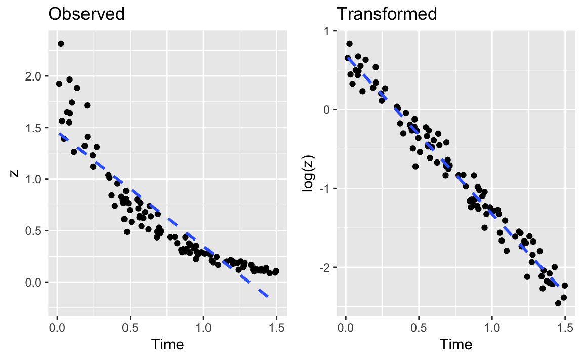
Figure 12-1 shows an example of exponential decay. The left panel shows the original data, z. The dotted line shows a linear regression on the original data; clearly, it’s a lousy fit. If the data is really exponential, then a possible model is:
where t is time and exp[⋅] is the exponential function (ex). This is not linear, of course, but we can linearize it by taking logarithms:
In R, that regression is simple because we can embed the log transform directly into the regression formula:
# read in our example dataload(file='./data/df_decay.rdata')z<-df_decay$zt<-df_decay$time# transform and modelm<-lm(log(z)~t)summary(m)#>#> Call:#> lm(formula = log(z) ~ t)#>#> Residuals:#> Min 1Q Median 3Q Max#> -0.4479 -0.0993 0.0049 0.0978 0.2802#>#> Coefficients:#> Estimate Std. Error t value Pr(>|t|)#> (Intercept) 0.6887 0.0306 22.5 <2e-16 ***#> t -2.0118 0.0351 -57.3 <2e-16 ***#> ---#> Signif. codes: 0 '***' 0.001 '**' 0.01 '*' 0.05 '.' 0.1 ' ' 1#>#> Residual standard error: 0.148 on 98 degrees of freedom#> Multiple R-squared: 0.971, Adjusted R-squared: 0.971#> F-statistic: 3.28e+03 on 1 and 98 DF, p-value: <2e-16
The right panel of Figure X-X shows the plot of log(z) versus time. Superimposed on that plot is their regression line. The fit appears to be much better; this is confirmed by the R2 = 0.97, compared with 0.82 for the linear regression on the original data.
You can embed other functions inside your formula. If you thought the relationship was quadratic, you could use a square-root transformation:
lm(sqrt(y)~month)
You can apply transformations to variables on both sides of the formula, of course. This formula regresses y on the square root of x:
lm(y~sqrt(x))
This regression is for a log-log relationship between x and y:
lm(log(y)~log(x))
You want to improve your linear model by applying a power transformation to the response variable.
Use the Box–Cox procedure, which is implemented by the boxcox function
of the MASS package. The procedure will identify a power, λ, such
that transforming y into yλ will improve the fit of your model:
library(MASS)m<-lm(y~x)boxcox(m)
To illustrate the Box–Cox transformation, let’s create some artificial data using the equation y−1.5 = x + ε, where ε is an error term:
set.seed(9)x<-10:100eps<-rnorm(length(x),sd=5)y<-(x+eps)^(-1/1.5)
Then we will (mistakenly) model the data using a simple linear regression and derive an adjusted R2 of 0.6374:
m<-lm(y~x)summary(m)#>#> Call:#> lm(formula = y ~ x)#>#> Residuals:#> Min 1Q Median 3Q Max#> -0.04032 -0.01633 -0.00792 0.00996 0.14516#>#> Coefficients:#> Estimate Std. Error t value Pr(>|t|)#> (Intercept) 0.166885 0.007078 23.6 <2e-16 ***#> x -0.001465 0.000116 -12.6 <2e-16 ***#> ---#> Signif. codes: 0 '***' 0.001 '**' 0.01 '*' 0.05 '.' 0.1 ' ' 1#>#> Residual standard error: 0.0291 on 89 degrees of freedom#> Multiple R-squared: 0.641, Adjusted R-squared: 0.637#> F-statistic: 159 on 1 and 89 DF, p-value: <2e-16
When plotting the residuals against the fitted values, we get a clue that something is wrong:
plot(m,which=1)# Plot only the fitted vs residuals
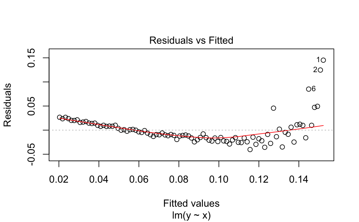
We used the Base R plot function to plot the residuals vs the fitted
values in Figure 12-2. We can see this plot has a clear
parabolic shape. A possible fix is a power transformation on y, so we
run the Box–Cox procedure:
library(MASS)#>#> Attaching package: 'MASS'#> The following object is masked from 'package:dplyr':#>#> selectbc<-boxcox(m)
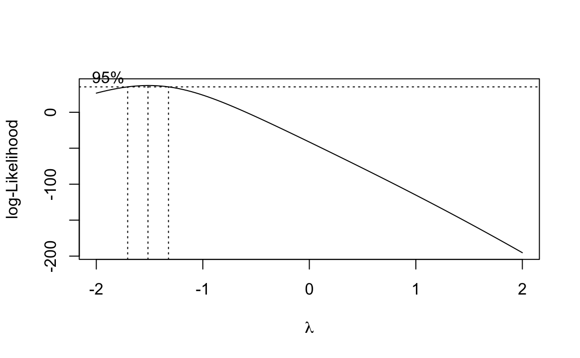
boxcox on the Model (m)The boxcox function plots values of λ against the log-likelihood of
the resulting model as shown in Figure 12-3. We want to maximize
that log-likelihood, so the function draws a line at the best value and
also draws lines at the limits of its confidence interval. In this case,
it looks like the best value is around −1.5, with a confidence interval
of about (−1.75, −1.25).
Oddly, the boxcox function does not return the best value of λ.
Rather, it returns the (x, y) pairs displayed in the plot. It’s
pretty easy to find the values of λ that yield the largest
log-likelihood y. We use the which.max function:
which.max(bc$y)#> [1] 13
Then this gives us the position of the corresponding λ:
lambda<-bc$x[which.max(bc$y)]lambda#> [1] -1.52
The function reports that the best λ is −1.515. In an actual application, We would urge you to interpret this number and choose the power that makes sense to you—rather than blindly accepting this “best” value. Use the graph to assist you in that interpretation. Here, We’ll go with −1.515.
We can apply the power transform to y and then fit the revised model; this gives a much better R2 of 0.9668:
z<-y^lambdam2<-lm(z~x)summary(m2)#>#> Call:#> lm(formula = z ~ x)#>#> Residuals:#> Min 1Q Median 3Q Max#> -13.459 -3.711 -0.228 2.206 14.188#>#> Coefficients:#> Estimate Std. Error t value Pr(>|t|)#> (Intercept) -0.6426 1.2517 -0.51 0.61#> x 1.0514 0.0205 51.20 <2e-16 ***#> ---#> Signif. codes: 0 '***' 0.001 '**' 0.01 '*' 0.05 '.' 0.1 ' ' 1#>#> Residual standard error: 5.15 on 89 degrees of freedom#> Multiple R-squared: 0.967, Adjusted R-squared: 0.967#> F-statistic: 2.62e+03 on 1 and 89 DF, p-value: <2e-16
For those who prefer one-liners, the transformation can be embedded right into the revised regression formula:
m2<-lm(I(y^lambda)~x)
By default, boxcox searches for values of λ in the range −2 to +2.
You can change that via the lambda argument; see the help page for
details.
We suggest viewing the Box–Cox result as a starting point, not as a definitive answer. If the confidence interval for λ includes 1.0, it may be that no power transformation is actually helpful. As always, inspect the residuals before and after the transformation. Did they really improve?
See Recipes “Regressing on Transformed Data” and “Diagnosing a Linear Regression”.
You are performing linear regression and you need the confidence intervals for the regression coefficients.
Save the regression model in an object; then use the confint function
to extract confidence intervals:
load(file='./data/conf.rdata')m<-lm(y~x1+x2)confint(m)#> 2.5 % 97.5 %#> (Intercept) -3.90 6.47#> x1 -2.58 6.24#> x2 4.67 5.17
The Solution uses the model y = β0 + β1(x1)i
β2(x2)i + εi. The confint function returns the
confidence intervals for the intercept (β0), the coefficient of
x1 (β1), and the coefficient of x2 (β2):
confint(m)#> 2.5 % 97.5 %#> (Intercept) -3.90 6.47#> x1 -2.58 6.24#> x2 4.67 5.17
By default, confint uses a confidence level of 95%. Use the level
parameter to select a different level:
confint(m,level=0.99)#> 0.5 % 99.5 %#> (Intercept) -5.72 8.28#> x1 -4.12 7.79#> x2 4.58 5.26
The coefplot function of the arm package can plot confidence
intervals for regression coefficients.
You want a visual display of your regression residuals.
You can plot the model object by selecting the residuals plot from the available plots:
m<-lm(y~x1+x2)plot(m,which=1)
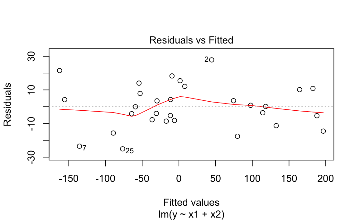
The output is shown in Figure 12-4.
Normally, plotting a regression model object produces several diagnostic
plots. You can select just the residuals plot by specifying which=1.
The graph above shows a plot of the residuals from “Performing Simple Linear Regression”. R draws a smoothed line through the residuals as a visual aid to finding significant patterns—for example, a slope or a parabolic shape.
See “Diagnosing a Linear Regression”, which contains examples of residuals plots and other diagnostic plots.
You have performed a linear regression. Now you want to verify the model’s quality by running diagnostic checks.
Start by plotting the model object, which will produce several diagnostic plots:
m<-lm(y~x1+x2)plot(m)
Next, identify possible outliers either by looking at the diagnostic
plot of the residuals or by using the outlierTest function of the
car package:
library(car)#> Loading required package: carData#>#> Attaching package: 'car'#> The following object is masked from 'package:dplyr':#>#> recode#> The following object is masked from 'package:purrr':#>#> someoutlierTest(m)#> No Studentized residuals with Bonferonni p < 0.05#> Largest |rstudent|:#> rstudent unadjusted p-value Bonferonni p#> 2 2.27 0.0319 0.956
Finally, identify any overly influential observations (“Identifying Influential Observations”).
R fosters the impression that linear regression is easy: just use the
lm function. Yet fitting the data is only the beginning. It’s your job
to decide whether the fitted model actually works and works well.
Before anything else, you must have a statistically significant model. Check the F statistic from the model summary (“Understanding the Regression Summary”) and be sure that the p-value is small enough for your purposes. Conventionally, it should be less than 0.05 or else your model is likely not very meaningful.
Simply plotting the model object produces several useful diagnostic plots, shown in Figure 12-5:
length(x1)#> [1] 30length(x2)#> [1] 30length(y)#> [1] 30m<-lm(y~x1+x2)par(mfrow=(c(2,2)))# this gives us a 2x2 plotplot(m)
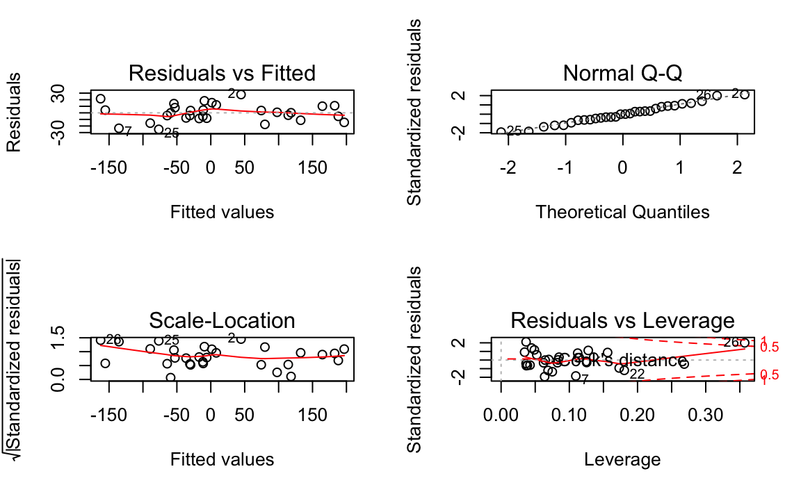
Figure 12-5 shows diagnostic plots for a pretty good regression:
The points in the Residuals vs Fitted plot are randomly scattered with no particular pattern.
The points in the Normal Q–Q plot are more-or-less on the line, indicating that the residuals follow a normal distribution.
In both the Scale–Location plot and the Residuals vs Leverage plots, the points are in a group with none too far from the center.
In contrast, the series of graphs shown in Figure 12-6 show the diagnostics for a not-so-good regression:
load(file='./data/bad.rdata')m<-lm(y2~x3+x4)par(mfrow=(c(2,2)))# this gives us a 2x2 plotplot(m)
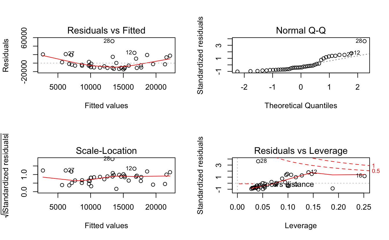
Observe that the Residuals vs Fitted plot has a definite parabolic shape. This tells us that the model is incomplete: a quadratic factor is missing that could explain more variation in y. Other patterns in residuals would be suggestive of additional problems: a cone shape, for example, may indicate nonconstant variance in y. Interpreting those patterns is a bit of an art, so we suggest reviewing a good book on linear regression while evaluating the plot of residuals.
There are other problems with the not-so-good diagnostics above. The Normal Q–Q plot has more points off the line than it does for the good regression. Both the Scale–Location and Residuals vs Leverage plots show points scattered away from the center, which suggests that some points have excessive leverage.
Another pattern is that point number 28 sticks out in every plot. This
warns us that something is odd with that observation. The point could be
an outlier, for example. We can check that hunch with the outlierTest
function of the car package:
outlierTest(m)#> rstudent unadjusted p-value Bonferonni p#> 28 4.46 7.76e-05 0.0031
The outlierTest identifies the model’s most outlying observation. In
this case, it identified observation number 28 and so confirmed that it
could be an outlier.
See recipes “Understanding the Regression Summary” and “Identifying Influential Observations”. The car
package is not part of the standard distribution of R; see “Installing Packages from CRAN”.
You want to identify the observations that are having the most influence on the regression model. This is useful for diagnosing possible problems with the data.
The influence.measures function reports several useful statistics for
identifying influential observations, and it flags the significant ones
with an asterisk (*). Its main argument is the model object from your
regression:
influence.measures(m)
The title of this recipe could be “Identifying Overly Influential Observations”, but that would be redundant. All observations influence the regression model, even if only a little. When a statistician says that an observation is influential, it means that removing the observation would significantly change the fitted regression model. We want to identify those observations because they might be outliers that distort our model; we owe it to ourselves to investigate them.
The influence.measures function reports several statistics: DFBETAS,
DFFITS, covariance ratio, Cook’s distance, and hat matrix values. If any
of these measures indicate that an observation is influential, the
function flags that observation with an asterisk (*) along the
righthand side:
influence.measures(m)#> Influence measures of#> lm(formula = y2 ~ x3 + x4) :#>#> dfb.1_ dfb.x3 dfb.x4 dffit cov.r cook.d hat inf#> 1 -0.18784 0.15174 0.07081 -0.22344 1.059 1.67e-02 0.0506#> 2 0.27637 -0.04367 -0.39042 0.45416 1.027 6.71e-02 0.0964#> 3 -0.01775 -0.02786 0.01088 -0.03876 1.175 5.15e-04 0.0772#> 4 0.15922 -0.14322 0.25615 0.35766 1.133 4.27e-02 0.1156#> 5 -0.10537 0.00814 -0.06368 -0.13175 1.078 5.87e-03 0.0335#> 6 0.16942 0.07465 0.42467 0.48572 1.034 7.66e-02 0.1062etc...
JDL NOTE: the output above does not seem to be respecting the output.lines=10 setting. Debug. We also use output.lines=5 in ch4. Go see if that is working
This is the model from “Diagnosing a Linear Regression”, where we suspected that observation 28 was an outlier. An asterisk is flagging that observation, confirming that it’s overly influential.
This recipe can identify influential observations, but you shouldn’t reflexively delete them. Some judgment is required here. Are those observations improving your model or damaging it?
See “Diagnosing a Linear Regression”. Use help(influence.measures) to get a list of influence
measures and some related functions. See a regression textbook for
interpretations of the various influence measures.
You have performed a linear regression and want to check the residuals for autocorrelation.
The Durbin—Watson test can check the residuals for autocorrelation. The
test is implemented by the dwtest function of the lmtest package:
library(lmtest)m<-lm(y~x)# Create a model objectdwtest(m)# Test the model residuals
The output includes a p-value. Conventionally, if p < 0.05 then the residuals are significantly correlated whereas p > 0.05 provides no evidence of correlation.
You can perform a visual check for autocorrelation by graphing the autocorrelation function (ACF) of the residuals:
acf(m)# Plot the ACF of the model residuals
The Durbin–Watson test is often used in time series analysis, but it was originally created for diagnosing autocorrelation in regression residuals. Autocorrelation in the residuals is a scourge because it distorts the regression statistics, such as the F statistic and the t statistics for the regression coefficients. The presence of autocorrelation suggests that your model is missing a useful predictor variable or that it should include a time series component, such as a trend or a seasonal indicator.
This first example builds a simple regression model and then tests the residuals for autocorrelation. The test returns a p-value well above zero, which indicates that there is no significant autocorrelation:
library(lmtest)#> Loading required package: zoo#>#> Attaching package: 'zoo'#> The following objects are masked from 'package:base':#>#> as.Date, as.Date.numericload(file='./data/ac.rdata')m<-lm(y1~x)dwtest(m)#>#> Durbin-Watson test#>#> data: m#> DW = 2, p-value = 0.4#> alternative hypothesis: true autocorrelation is greater than 0
This second example exhibits autocorrelation in the residuals. The p-value is near 0, so the autocorrelation is likely positive:
m<-lm(y2~x)dwtest(m)#>#> Durbin-Watson test#>#> data: m#> DW = 2, p-value = 0.01#> alternative hypothesis: true autocorrelation is greater than 0
By default, dwtest performs a one-sided test and answers this
question: Is the autocorrelation of the residuals greater than zero? If
your model could exhibit negative autocorrelation (yes, that is
possible), then you should use the alternative option to perform a
two-sided test:
dwtest(m,alternative="two.sided")
The Durbin–Watson test is also implemented by the durbinWatsonTest
function of the car package. We suggested the dwtest function
primarily because we think the output is easier to read.
Neither the lmtest package nor the car package are included in the
standard distribution of R; see recipes @ref(recipe-id013) “Accessing the Functions in a Package” and @ref(recipe-id012) “Installing Packages from CRAN”.
See recipes @ref(recipe-id082) X-X and X-X
for more regarding tests of autocorrelation.
You want to predict new values from your regression model.
Save the predictor data in a data frame. Use the predict function,
setting the newdata parameter to the data frame:
load(file='./data/pred2.rdata')m<-lm(y~u+v+w)preds<-data.frame(u=3.1,v=4.0,w=5.5)predict(m,newdata=preds)#> 1#> 45
Once you have a linear model, making predictions is quite easy because
the predict function does all the heavy lifting. The only annoyance is
arranging for a data frame to contain your data.
The predict function returns a vector of predicted values with one
prediction for every row in the data. The example in the Solution
contains one row, so predict returned one value.
If your predictor data contains several rows, you get one prediction per row:
preds<-data.frame(u=c(3.0,3.1,3.2,3.3),v=c(3.9,4.0,4.1,4.2),w=c(5.3,5.5,5.7,5.9))predict(m,newdata=preds)#> 1 2 3 4#> 43.8 45.0 46.3 47.5
In case it’s not obvious: the new data needn’t contain values for response variables, only predictor variables. After all, you are trying to calculate the response, so it would be unreasonable of R to expect you to supply it.
These are just the point estimates of the predictions. See “Forming Prediction Intervals” for the confidence intervals.
You are making predictions using a linear regression model. You want to know the prediction intervals: the range of the distribution of the prediction.
Use the predict function and specify interval="prediction":
predict(m,newdata=preds,interval="prediction")
This is a continuation of “Predicting New Values”,
which described packaging your data into a data frame for the predict
function. We are adding interval="prediction" to obtain prediction
intervals.
Here is the example from “Predicting New Values”, now
with prediction intervals. The new lwr and upr columns are the lower
and upper limits, respectively, for the interval:
predict(m,newdata=preds,interval="prediction")#> fit lwr upr#> 1 43.8 38.2 49.4#> 2 45.0 39.4 50.7#> 3 46.3 40.6 51.9#> 4 47.5 41.8 53.2
By default, predict uses a confidence level of 0.95. You can change
this via the level argument.
A word of caution: these prediction intervals are extremely sensitive to deviations from normality. If you suspect that your response variable is not normally distributed, consider a nonparametric technique, such as the bootstrap (Recipe X-X), for prediction intervals.
Your data is divided into groups, and the groups are normally distributed. You want to know if the groups have significantly different means.
Use a factor to define the groups. Then apply the oneway.test
function:
oneway.test(x~f)
Here, x is a vector of numeric values and f is a factor that
identifies the groups. The output includes a p-value. Conventionally,
a p-value of less than 0.05 indicates that two or more groups have
significantly different means whereas a value exceeding 0.05 provides no
such evidence.
Comparing the means of groups is a common task. One-way ANOVA performs that comparison and computes the probability that they are statistically identical. A small p-value indicates that two or more groups likely have different means. (It does not indicate that all groups have different means.)
The basic ANOVA test assumes that your data has a normal distribution or that, at least, it is pretty close to bell-shaped. If not, use the Kruskal–Wallis test instead (“Performing Robust ANOVA (Kruskal–Wallis Test)”).
We can illustrate ANOVA with stock market historical data. Is the stock
market more profitable in some months than in others? For instance, a
common folk myth says that October is a bad month for stock market
investors.1 We explored this question by creating a
data frame GSPC_df containing two columns, r and mon. r, is the
daily returns in the Standard & Poor’s 500 index, a broad measure of
stock market performance. The factor, mon, indicates the calendar
month in which that change occurred: Jan, Feb, Mar, and so forth. The
data covers the period 1950 though 2009.
The one-way ANOVA shows a p-value of 0.03347:
load(file='./data/anova.rdata')oneway.test(r~mon,data=GSPC_df)#>#> One-way analysis of means (not assuming equal variances)#>#> data: r and mon#> F = 2, num df = 10, denom df = 7000, p-value = 0.03
We can conclude that stock market changes varied significantly according to the calendar month.
Before you run to your broker and start flipping your portfolio monthly,
however, we should check something: did the pattern change recently? We
can limit the analysis to recent data by specifying a subset
parameter. This works for oneway.test just as it does for the lm
function. The subset contains the indexes of observations to be
analyzed; all other observations are ignored. Here, we give the indexes
of the 2,500 most recent observations, which is about 10 years of data:
oneway.test(r~mon,data=GSPC_df,subset=tail(seq_along(r),2500))#>#> One-way analysis of means (not assuming equal variances)#>#> data: r and mon#> F = 0.7, num df = 10, denom df = 1000, p-value = 0.8
Uh-oh! Those monthly differences evaporated during the past 10 years. The large p-value, 0.7608, indicates that changes have not recently varied according to calendar month. Apparently, those differences are a thing of the past.
Notice that the oneway.test output says “(not assuming equal
variances)”. If you know the groups have equal variances, you’ll get a
less conservative test by specifying var.equal=TRUE:
oneway.test(x~f,var.equal=TRUE)
You can also perform one-way ANOVA by using the aov function like
this:
m<-aov(x~f)summary(m)
However, the aov function always assumes equal variances and so is
somewhat less flexible than oneway.test.
If the means are significantly different, use “Finding Differences Between Means of Groups” to see the actual differences. Use “Performing Robust ANOVA (Kruskal–Wallis Test)” if your data is not normally distributed, as required by ANOVA.
You are performing multiway ANOVA: using two or more categorical variables as predictors. You want a visual check of possible interaction between the predictors.
Use the interaction.plot function:
interaction.plot(pred1,pred2,resp)
Here, pred1 and pred2 are two categorical predictors and resp is
the response variable.
ANOVA is a form of linear regression, so ideally there is a linear relationship between every predictor and the response variable. One source of nonlinearity is an interaction between two predictors: as one predictor changes value, the other predictor changes its relationship to the response variable. Checking for interaction between predictors is a basic diagnostic.
The faraway package contains a dataset called rats. In it, treat
and poison are categorical variables and time is the response
variable. When plotting poison against time we are looking for
straight, parallel lines, which indicate a linear relationship. However,
using the interaction.plot function produces Figure 12-7 which reveals that something is not right:
library(faraway)data(rats)interaction.plot(rats$poison,rats$treat,rats$time)
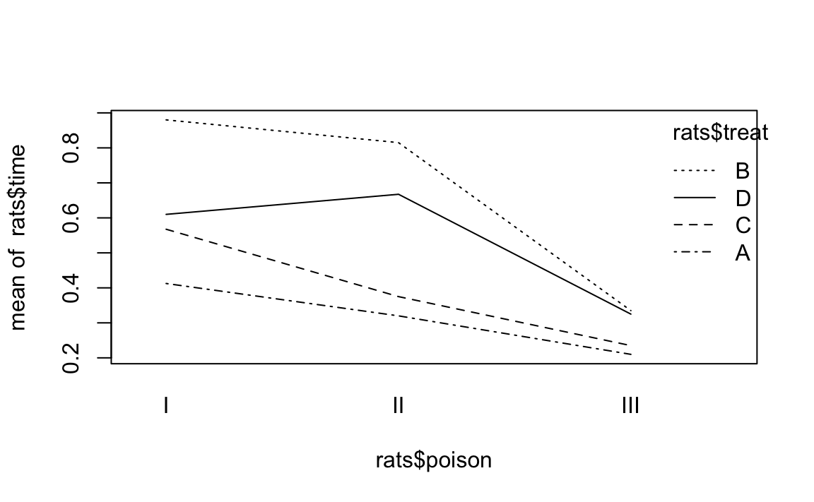
Each line graphs time against poison. The difference between lines
is that each line is for a different value of treat. The lines should
be parallel, but the top two are not exactly parallel. Evidently,
varying the value of treat “warped” the lines, introducing a
nonlinearity into the relationship between poison and time.
This signals a possible interaction that we should check. For this data it just so happens that yes, there is an interaction but no, it is not statistically significant. The moral is clear: the visual check is useful, but it’s not foolproof. Follow up with a statistical check.
Your data is divided into groups, and an ANOVA test indicates that the groups have significantly different means. You want to know the differences between those means for all groups.
Perform the ANOVA test using the aov function, which returns a model
object. Then apply the TukeyHSD function to the model object:
m<-aov(x~f)TukeyHSD(m)
Here, x is your data and f is the grouping factor. You can plot the
TukeyHSD result to obtain a graphical display of the differences:
plot(TukeyHSD(m))
The ANOVA test is important because it tells you whether or not the groups’ means are different. But the test does not identify which groups are different, and it does not report their differences.
The TukeyHSD function can calculate those differences and help you
identify the largest ones. It uses the “honest significant differences”
method invented by John Tukey.
We’ll illustrate TukeyHSD by continuing the example from
“Performing One-Way ANOVA”, which grouped daily stock
market changes by month. Here, we group them by weekday instead, using a
factor called wday that identifies the day of the week (Mon, …, Fri)
on which the change occurred. We’ll use the first 2,500 observations,
which roughly cover the period from 1950 to 1960:
load(file='./data/anova.rdata')oneway.test(r~wday,subset=1:2500,data=GSPC_df)#>#> One-way analysis of means (not assuming equal variances)#>#> data: r and wday#> F = 10, num df = 4, denom df = 1000, p-value = 5e-10
The p-value is essentially zero, indicating that average changes
varied significantly depending on the weekday. To use the TukeyHSD
function, We first perform the ANOVA test using the aov function,
which returns a model object, and then apply the TukeyHSD function to
the object:
m<-aov(r~wday,subset=1:2500,data=GSPC_df)TukeyHSD(m)#> Tukey multiple comparisons of means#> 95% family-wise confidence level#>#> Fit: aov(formula = r ~ wday, data = GSPC_df, subset = 1:2500)#>#> $wday#> diff lwr upr p adj#> Mon-Fri -0.003153 -4.40e-03 -0.001911 0.000#> Thu-Fri -0.000934 -2.17e-03 0.000304 0.238#> Tue-Fri -0.001855 -3.09e-03 -0.000618 0.000#> Wed-Fri -0.000783 -2.01e-03 0.000448 0.412#> Thu-Mon 0.002219 9.79e-04 0.003460 0.000#> Tue-Mon 0.001299 5.85e-05 0.002538 0.035#> Wed-Mon 0.002370 1.14e-03 0.003605 0.000#> Tue-Thu -0.000921 -2.16e-03 0.000314 0.249#> Wed-Thu 0.000151 -1.08e-03 0.001380 0.997#> Wed-Tue 0.001072 -1.57e-04 0.002300 0.121
Each line in the output table includes the difference between the means
of two groups (diff) as well as the lower and upper bounds of the
confidence interval (lwr and upr) for the difference. The first line
in the table, for example,compares the Mon group and the Fri group: the
difference of their means is 0.003 with a confidence interval of
(-0.0044 -0.0019).
Scanning the table, we see that the Wed-Mon comparison had the largest difference, which was 0.00237.
A cool feature of TukeyHSD is that it can display these differences
visually, too. Simply plot the function’s return value to get output as
is shown in Figure 12-8.
plot(TukeyHSD(m))
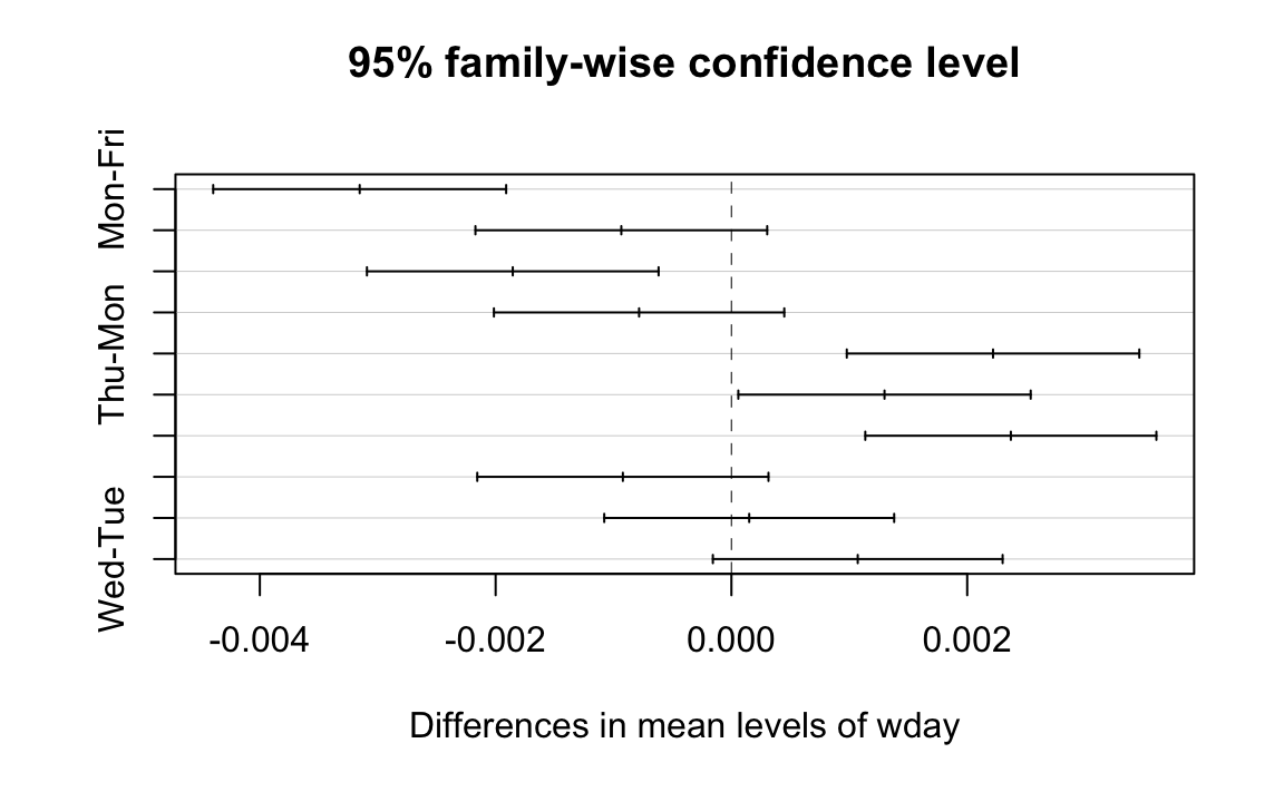
The horizontal lines plot the confidence intervals for each pair. With this visual representation you can quickly see that several confidence intervals cross over zero, indicating that the difference is not necessarily significant. You can also see that the Wed-Mon pair has the largest difference because their confidence interval is farthest to the right.
Your data is divided into groups. The groups are not normally distributed, but their distributions have similar shapes. You want to perform a test similar to ANOVA—you want to know if the group medians are significantly different.
Create a factor that defines the groups of your data. Use the
kruskal.test function, which implements the Kruskal–Wallis test.
Unlike the ANOVA test, this test does not depend upon the normality of
the data:
kruskal.test(x~f)
Here, x is a vector of data and f is a grouping factor. The output
includes a p-value. Conventionally, p < 0.05 indicates that there is
a significant difference between the medians of two or more groups
whereas p > 0.05 provides no such evidence.
Regular ANOVA assumes that your data has a Normal distribution. It can tolerate some deviation from normality, but extreme deviations will produce meaningless p-values.
The Kruskal–Wallis test is a nonparametric version of ANOVA, which means that it does not assume normality. However, it does assume same-shaped distributions. You should use the Kruskal–Wallis test whenever your data distribution is nonnormal or simply unknown.
The null hypothesis is that all groups have the same median. Rejecting the null hypothesis (with p < 0.05) does not indicate that all groups are different, but it does suggest that two or more groups are different.
One year, Paul taught Business Statistics to 94 undergraduate students. The class included a midterm examination, and there were four homework assignments prior to the exam. He wanted to know: What is the relationship between completing the homework and doing well on the exam? If there is no relation, then the homework is irrelevant and needs rethinking.
He created a vector of grades, one per student and he also created a
parallel factor that captured the number of homework assignments
completed by that student. The data are in a data frame named
student_data:
load(file='./data/student_data.rdata')head(student_data)#> # A tibble: 6 x 4#> att.fact hw.mean midterm hw#> <fct> <dbl> <dbl> <fct>#> 1 3 0.808 0.818 4#> 2 3 0.830 0.682 4#> 3 3 0.444 0.511 2#> 4 3 0.663 0.670 3#> 5 2 0.9 0.682 4#> 6 3 0.948 0.954 4
Notice that the hw variable—although it appears to be numeric—is
actually a factor. It assigns each midterm grade to one of five groups
depending upon how many homework assignments the student completed.
The distribution of exam grades is definitely not Normal: the students have a wide range of math skills, so there are an unusual number of A and F grades. Hence regular ANOVA would not be appropriate. Instead we used the Kruskal–Wallis test and obtained a p-value of essentially zero (3.99 × 10⁻⁵, or 0.00003669):
kruskal.test(midterm~hw,data=student_data)#>#> Kruskal-Wallis rank sum test#>#> data: midterm by hw#> Kruskal-Wallis chi-squared = 30, df = 4, p-value = 4e-05
Obviously, there is a significant performance difference between students who complete their homework and those who do not. But what could Paul actually conclude? At first, Paul was pleased that the homework appeared so effective. Then it dawned on him that this was a classic error in statistical reasoning: He assumed that correlation implied causality. It does not, of course. Perhaps strongly motivated students do well on both homework and exams whereas lazy students do not. In that case, the causal factor is degree of motivation, not the brilliance of my homework selection. In the end, he could only conclude something very simple: students who complete the homework will likely do well on the midterm exam, but he still doesn’t really know why.
You have two models of the same data, and you want to know whether they produce different results.
The anova function can compare two models and report if they are
significantly different:
anova(m1,m2)
Here, m1 and m2 are both model objects returned by lm. The output
from anova includes a p-value. Conventionally, a p-value of less
than 0.05 indicates that the models are significantly different whereas
a value exceeding 0.05 provides no such evidence.
In “Getting Regression Statistics”, we used the
anova function to print the ANOVA table for one regression model. Now
we are using the two-argument form to compare two models.
The anova function has one strong requirement when comparing two
models: one model must be contained within the other. That is, all the
terms of the smaller model must appear in the larger model. Otherwise,
the comparison is impossible.
The ANOVA analysis performs an F test that is similar to the F test for a linear regression. The difference is that this test is between two models whereas the regression F test is between using the regression model and using no model.
Suppose we build three models of y, adding terms as we go:
load(file='./data/anova2.rdata')m1<-lm(y~u)m2<-lm(y~u+v)m3<-lm(y~u+v+w)
Is m2 really different from m1? We can use anova to compare them,
and the result is a p-value of 0.009066:
anova(m1,m2)#> Analysis of Variance Table#>#> Model 1: y ~ u#> Model 2: y ~ u + v#> Res.Df RSS Df Sum of Sq F Pr(>F)#> 1 18 197#> 2 17 130 1 66.4 8.67 0.0091 **#> ---#> Signif. codes: 0 '***' 0.001 '**' 0.01 '*' 0.05 '.' 0.1 ' ' 1
The small p-value indicates that the models are significantly
different. Comparing m2 and m3, however, yields a p-value of
0.05527:
anova(m2,m3)#> Analysis of Variance Table#>#> Model 1: y ~ u + v#> Model 2: y ~ u + v + w#> Res.Df RSS Df Sum of Sq F Pr(>F)#> 1 17 130#> 2 16 103 1 27.5 4.27 0.055 .#> ---#> Signif. codes: 0 '***' 0.001 '**' 0.01 '*' 0.05 '.' 0.1 ' ' 1
This is right on the edge. Strictly speaking, it does not pass our requirement to be smaller than 0.05; however, it’s close enough that you might judge the models to be “different enough.”
This example is a bit contrived, so it does not show the larger power of
anova. We use anova when, while experimenting with complicated
models by adding and deleting multiple terms, we need to know whether or
not the new model is really different from the original one. In other
words: if we add terms and the new model is essentially unchanged, then
the extra terms are not worth the additional complications.
1 In the words of Mark Twain, “October: This is one of the peculiarly dangerous months to speculate in stocks in. The others are July, January, September, April, November, May, March, June, December, August and February.”
Second Edition
Proven Recipes for Data Analysis, Statistics, and Graphics
Copyright © 2019 J.D. Long and Paul Teetor. All rights reserved.
Printed in the United States of America.
Published by O’Reilly Media, Inc., 1005 Gravenstein Highway North, Sebastopol, CA 95472.
O’Reilly books may be purchased for educational, business, or sales promotional use. Online editions are also available for most titles (http://oreilly.com/safari). For more information, contact our corporate/institutional sales department: 800-998-9938 or corporate@oreilly.com.
See http://oreilly.com/catalog/errata.csp?isbn=9781492040682 for release details.
The O’Reilly logo is a registered trademark of O’Reilly Media, Inc. R Cookbook, the cover image, and related trade dress are trademarks of O’Reilly Media, Inc.
While the publisher and the author have used good faith efforts to ensure that the information and instructions contained in this work are accurate, the publisher and the author disclaim all responsibility for errors or omissions, including without limitation responsibility for damages resulting from the use of or reliance on this work. Use of the information and instructions contained in this work is at your own risk. If any code samples or other technology this work contains or describes is subject to open source licenses or the intellectual property rights of others, it is your responsibility to ensure that your use thereof complies with such licenses and/or rights.
978-1-492-04068-2
This chapter sets the groundwork for the other chapters. It explains how to download, install, and run R.
More importantly, it also explains how to get answers to your questions. The R community provides a wealth of documentation and help. You are not alone. Here are some common sources of help:
When you install R on your computer, a mass of documentation is also installed. You can browse the local documentation (“Viewing the Supplied Documentation”) and search it (“Searching the Supplied Documentation”). We are amazed how often we search the Web for an answer only to discover it was already available in the installed documentation.
A task view describes packages that are specific to one area of statistical work, such as econometrics, medical imaging, psychometrics, or spatial statistics. Each task view is written and maintained by an expert in the field. There are more than 35 such task views, so there is likely to be one or more for your areas of interest. We recommend that every beginner find and read at least one task view in order to gain a sense of R’s possibilities (“Finding Relevant Functions and Packages”).
Most packages include useful documentation. Many also include overviews and tutorials, called “vignettes” in the R community. The documentation is kept with the packages in package repositories, such as CRAN (http://cran.r-project.org/), and it is automatically installed on your machine when you install a package.
On a Q&A site, anyone can post a question, and knowledgeable people can respond. Readers vote on the answers, so the best answers tend to emerge over time. All this information is tagged and archived for searching. These sites are a cross between a mailing list and a social network; “Stack Overflow” (http://stackoverflow.com/) is the canonical example.
The Web is loaded with information about R, and there are R-specific tools for searching it (“Searching the Web for Help”). The Web is a moving target, so be on the lookout for new, improved ways to organize and search information regarding R.
Volunteers have generously donated many hours of time to answer beginners’ questions that are posted to the R mailing lists. The lists are archived, so you can search the archives for answers to your questions (“Searching the Mailing Lists”).
You want to install R on your computer.
Windows and OS X users can download R from CRAN, the Comprehensive R Archive Network. Linux and Unix users can install R packages using their package management tool:
Windows
Open http://www.r-project.org/ in your browser.
Click on “CRAN”. You’ll see a list of mirror sites, organized by country.
Select a site near you or the top one listed as “0-Cloud” which tends to work well for most locations (https://cloud.r-project.org/)
Click on “Download R for Windows” under “Download and Install R”.
Click on “base”.
Click on the link for downloading the latest version of R (an .exe
file).
When the download completes, double-click on the .exe file and
answer the usual questions.
OS X
Open http://www.r-project.org/ in your browser.
Click on “CRAN”. You’ll see a list of mirror sites, organized by country.
Select a site near you or the top one listed as “0-Cloud” which tends to work well for most locations.
Click on “Download R for (Mac) OS X”.
Click on the .pkg file for the latest version of R, under “Latest
release:”, to download it.
When the download completes, double-click on the .pkg file and
answer the usual questions.
Linux or Unix
The major Linux distributions have packages for installing R. Here are some examples:
| Distribution | Package name |
|---|---|
Ubuntu or Debian |
r-base |
Red Hat or Fedora |
R.i386 |
Suse |
R-base |
Use the system’s package manager to download and install the package.
Normally, you will need the root password or sudo privileges;
otherwise, ask a system administrator to perform the installation.
Installing R on Windows or OS X is straightforward because there are prebuilt binaries (compiled programs) for those platforms. You need only follow the preceding instructions. The CRAN Web pages also contain links to installation-related resources, such as frequently asked questions (FAQs) and tips for special situations (“Does R run under Windows Vista/7/8/Server 2008?”) that you may find useful.
The best way to install R on Linux or Unix is by using your Linux distribution package manager to install R as a package. The distribution packages greatly streamline both the initial installation and subsequent updates.
On Ubuntu or Debian, use apt-get to download and install R. Run under
sudo to have the necessary privileges:
$sudoapt-getinstallr-base
On Red Hat or Fedora, use yum:
$sudoyuminstallR.i386
Most Linux platforms also have graphical package managers, which you might find more convenient.
Beyond the base packages, we recommend installing the documentation
packages, too. We like to install r-base-html (because we like
browsing the hyperlinked documentation) as well as r-doc-html, which
installs the important R manuals locally:
$sudoapt-getinstallr-base-htmlr-doc-html
Some Linux repositories also include prebuilt copies of R packages available on CRAN. We don’t use them because we’d rather get software directly from CRAN itself, which usually has the freshest versions.
In rare cases, you may need to build R from scratch. You might have an
obscure, unsupported version of Unix; or you might have special
considerations regarding performance or configuration. The build
procedure on Linux or Unix is quite standard. Download the tarball from
the home page of your CRAN mirror; it’s called something like
R-3.5.1.tar.gz, except the “3.5.1” will be replaced by the latest
version. Unpack the tarball, look for a file called INSTALL, and
follow the directions.
R in a Nutshell (http://oreilly.com/catalog/9780596801717) (O’Reilly) contains more details of downloading and installing R, including instructions for building the Windows and OS X versions. Perhaps the ultimate guide is the one entitled “R Installation and Administration” (http://cran.r-project.org/doc/manuals/R-admin.html), available on CRAN, which describes building and installing R on a variety of platforms.
This recipe is about installing the base package. See “Installing Packages from CRAN” for installing add-on packages from CRAN.
You want a more comprehensive Integrated Development Environment (IDE) than the R default. In other words, you want to install R Studio Desktop.
Over the past few years R Studio has become the most widly used IDE for
R. We are of the opinion that most all R work should be done in the R
Studio Desktop IDE unless there is a compelling reason to do otherwise.
R Studio makes multiple products including R Studio Desktop, R Studio
Server, R Studio Shiny Server, just to name a few. For this book we will
use the term R Studio to mean R Studio Desktop though most concepts
apply to R Studio Server as well.
To install R Studio, download the latest installer for your platform from the R Studio website: https://www.rstudio.com/products/rstudio/download/
The R Studio Desktop Open Source License version is free to download and use.
This book was written and built using R Studio version 1.2.x and R versions 3.5.x. New versions of R Studio are released every few months, so be sure and update regularly. Note that R Studio works with whichever version of R you have installed. So updating to the latest version of R Studio does not upgrade your version of R. R must be upgraded seperatly.
Interacting with R is slightly different in R Studio than in the built in R user interface. For this book, we’ve elected to use R Studio for all examples.
You want to run R Studio on your computer.
A common point of confusion for new users of R and R Studio is to
accidentally start R when they intended to start R Studio. The easiest
way to ensure you’re actually starting R Studio is to search for
RStudio on your desktop OS. Then use whatever method your OS provides
for pinning the icon somewhere easy to find later.
Click on the Start Screen menue in the lower left corner of the
screen. In the search box, type RStudio.
Look in your launchpad for the R Studio app or press command
space and type Rstudio to search using Spotlight Search.
Press Alt + F1 and type RStudio to search for R Studio.
Confusion between R and R Studio can easily happen becuase as you can see in Figure 1-1, the icons look similiar.
If you click on the R icon you’ll be greeted by something like Figure
Figure 1-2 which is the Base R interface on a Mac, but certainly
not R Studio.
When you start R Studio, the default behavior is that R Studio will reopen the last project you were working on in R Studio.
You’ve started R Studio. Now what?
When you start R Studio, the main window on the left is an R session. From there you can enter commands interactivly directly to R.
R prompts you with “>”. To get started, just treat R like a big
calculator: enter an expression, and R will evaluate the expression and
print the result:
1+1#> [1] 2
The computer adds one and one, giving two, and displays the result.
The [1] before the 2 might be confusing. To R, the result is a
vector, even though it has only one element. R labels the value with
[1] to signify that this is the first element of the vector… which
is not surprising, since it’s the only element of the vector.
R will prompt you for input until you type a complete expression. The
expression max(1,3,5) is a complete expression, so R stops reading
input and evaluates what it’s got:
max(1,3,5)#> [1] 5
In contrast, “max(1,3,” is an incomplete expression, so R prompts you
for more input. The prompt changes from greater-than (>) to plus
(+), letting you know that R expects more:
max(1,3,+5)#> [1] 5
It’s easy to mistype commands, and retyping them is tedious and frustrating. So R includes command-line editing to make life easier. It defines single keystrokes that let you easily recall, correct, and reexecute your commands. My own typical command-line interaction goes like this:
I enter an R expression with a typo.
R complains about my mistake.
I press the up-arrow key to recall my mistaken line.
I use the left and right arrow keys to move the cursor back to the error.
I use the Delete key to delete the offending characters.
I type the corrected characters, which inserts them into the command line.
I press Enter to reexecute the corrected command.
That’s just the basics. R supports the usual keystrokes for recalling and editing command lines, as listed in table @ref(tab:keystrokes).
| Labeled key | Ctrl-key combination | Effect |
|---|---|---|
Up arrow |
Ctrl-P |
Recall previous command by moving backward through the history of commands. |
Down arrow |
Ctrl-N |
Move forward through the history of commands. |
Backspace |
Ctrl-H |
Delete the character to the left of cursor. |
Delete (Del) |
Ctrl-D |
Delete the character to the right of cursor. |
Home |
Ctrl-A |
Move cursor to the start of the line. |
End |
Ctrl-E |
Move cursor to the end of the line. |
Right arrow |
Ctrl-F |
Move cursor right (forward) one character. |
Left arrow |
Ctrl-B |
Move cursor left (back) one character. |
Ctrl-K |
Delete everything from the cursor position to the end of the line. |
|
Ctrl-U |
Clear the whole darn line and start over. |
|
Tab |
Name completion (on some platforms). |
: Keystrokes for command-line editing
On Windows and OS X, you can also use the mouse to highlight commands and then use the usual copy and paste commands to paste text into a new command line.
See “Typing Less and Accomplishing More”. From the Windows main menu, follow Help →
Console for a complete list of keystrokes useful for command-line
editing.
You want to exit from R Studio.
Select File → Quit Session from the main menu; or click on the X
in the upper-right corner of the window frame.
Press CMD-q (apple-q); or click on the red X in the upper-left corner of the window frame.
At the command prompt, press Ctrl-D.
On all platforms, you can also use the q function (as in _q_uit) to
terminate the program.
q()
Note the empty parentheses, which are necessary to call the function.
Whenever you exit, R typically asks if you want to save your workspace. You have three choices:
Save your workspace and exit.
Don’t save your workspace, but exit anyway.
Cancel, returning to the command prompt rather than exiting.
If you save your workspace, then R writes it to a file called .RData
in the current working directory. Savign the workspace saves any R
objects which you have created. Next time you start R in the same
directory the workspace will automatically load. Saving your workspace
will overwrite the previously saved workspace, if any, so don’t save if
you don’t like the changes to your workspace (e.g., if you have
accidentally erased critical data).
We recommend never saving your workspace when you exit, and instead
always explicitly saving your project, scripts, and data. We also
recommend that you turn off the prompt to save and auto restore of
workspace in R Studio using the Global Options found in the menu Tools
→ Global Options and shown in Figure 1-3. This way
when you exit R and R Studio you will not be prompted to save your
workspace. But keep in mind that any objects created but not saved to
disk will be lost.
See “Getting and Setting the Working Directory” for more about the current working directory and “Saving Your Workspace” for more about saving your workspace. See Chapter 2 of R in a Nutshell (http://oreilly.com/catalog/9780596801717).
You want to interrupt a long-running computation and return to the command prompt without exiting R Studio.
Press the Esc key on your keyboard, or click on the Session Menu in
R Studio and select Interrupt R
Interrupting R means telling R to stop running the current command but without deleting variables from memory or completly closing R Studio. Although, interrupting R can leave your variables in an indeterminate state, depending upon how far the computation had progressed. Check your workspace after interrupting.
You want to read the documentation supplied with R.
Use the help.start function to see the documentation’s table of
contents:
help.start()
From there, links are available to all the installed documentation. In R Studio the help will show up in the help pane which by default is on the right hand side of the screen.
In R Studio you can also click help → R Help to get a listng with
help options for both R and R Studio.
The base distribution of R includes a wealth of documentation—literally thousands of pages. When you install additional packages, those packages contain documentation that is also installed on your machine.
It is easy to browse this documentation via the help.start function,
which opens on the top-level table of contents. Figure
Figure 1-4 shows how help.start() appears inside the help
pane in R Studio.
The two links in the Base R Reference section are especially useful:
Click here to see a list of all the installed packages, both in the base packages and the additional, installed packages. Click on a package name to see a list of its functions and datasets.
Click here to access a simple search engine, which allows you to search the documentation by keyword or phrase. There is also a list of common keywords, organized by topic; click one to see the associated pages.
The Base R documentation shown by typing help.start() is loaded on
your computer when you install R. The R Studio help which you get by
using the menu option help → R Help presents a page with links to R
Studio’s web site. So you will need Internet access to access the R
Studio help links.
The local documentation is copied from the R Project website, which may have updated documents.
You want to know more about a function that is installed on your machine.
Use help to display the documentation for the function:
help(functionname)
Use args for a quick reminder of the function arguments:
args(functionname)
Use example to see examples of using the function:
example(functionname)
We present many R functions in this book. Every R function has more bells and whistles than we can possibly describe. If a function catches your interest, we strongly suggest reading the help page for that function. One of its bells or whistles might be very useful to you.
Suppose you want to know more about the mean function. Use the help
function like this:
help(mean)
This will open the help page for the mean function in the help pane in R
Studio. A shortcut for the help command is to simply type ? followed
by the function name:
?mean
Sometimes you just want a quick reminder of the arguments to a function:
What are they, and in what order do they occur? Use the args function:
args(mean)#> function (x, ...)#> NULL
args(sd)#> function (x, na.rm = FALSE)#> NULL
The first line of output from args is a synopsis of the function call.
For mean, the synopsis shows one argument, x, which is a vector of
numbers. For sd, the synopsis shows the same vector, x, and an
optional argument called na.rm. (You can ignore the second line of
output, which is often just NULL.) In R Studio you will see the args
output as a floating tool tip over your cursor when you type a function
name as shown in figure Figure 1-5.
Most documentation for functions includes example code near the end of
the document. A cool feature of R is that you can request that it
execute the examples, giving you a little demonstration of the
function’s capabilities. The documentation for the mean function, for
instance, contains examples, but you don’t need to type them yourself.
Just use the example function to watch them run:
example(mean)#>#> mean> x <- c(0:10, 50)#>#> mean> xm <- mean(x)#>#> mean> c(xm, mean(x, trim = 0.10))#> [1] 8.75 5.50
The user typed example(mean). Everything else was produced by R, which
executed the examples from the help page and displayed the results.
See “Searching the Supplied Documentation” for searching for functions and “Displaying Loaded Packages via the Search Path” for more about the search path.
You want to know more about a function that is installed on your
machine, but the help function reports that it cannot find
documentation for any such function.
Alternatively, you want to search the installed documentation for a keyword.
Use help.search to search the R documentation on your computer:
help.search("pattern")
A typical pattern is a function name or keyword. Notice that it must be enclosed in quotation marks.
For your convenience, you can also invoke a search by using two question marks (in which case the quotes are not required). Note that searching for a function by name uses one question mark while searching for a text pattern uses two:
>??pattern
You may occasionally request help on a function only to be told R knows nothing about it:
help(adf.test)#> No documentation for 'adf.test' in specified packages and libraries:#> you could try '??adf.test'
This can be frustrating if you know the function is installed on your machine. Here the problem is that the function’s package is not currently loaded, and you don’t know which package contains the function. It’s a kind of catch-22 (the error message indicates the package is not currently in your search path, so R cannot find the help file; see “Displaying Loaded Packages via the Search Path” for more details).
The solution is to search all your installed packages for the function.
Just use the help.search function, as suggested in the error message:
help.search("adf.test")
The search will produce a listing of all packages that contain the function:
Helpfileswithaliasorconceptortitlematching'adf.test'usingregularexpressionmatching:tseries::adf.testAugmentedDickey-FullerTestType'?PKG::FOO'toinspectentry'PKG::FOO TITLE'.
The output above indicates that the tseries package contains the
adf.test function. You can see its documentation by explicitly telling
help which package contains the function:
help(adf.test,package="tseries")
or you can use the double colon operator to tell R to look in a specific package:
?tseries::adf.test
You can broaden your search by using keywords. R will then find any installed documentation that contains the keywords. Suppose you want to find all functions that mention the Augmented Dickey–Fuller (ADF) test. You could search on a likely pattern:
help.search("dickey-fuller")
On my machine, the result looks like this because I’ve installed two
additional packages (fUnitRoots and urca) that implement the ADF
test:
Helpfileswithaliasorconceptortitlematching'dickey-fuller'usingfuzzymatching:fUnitRoots::DickeyFullerPValuesDickey-FullerpValuestseries::adf.testAugmentedDickey-FullerTesturca::ur.dfAugmented-Dickey-FullerUnitRootTestType'?PKG::FOO'toinspectentry'PKG::FOO TITLE'.
You can also access the local search engine through the documentation browser; see “Viewing the Supplied Documentation” for how this is done. See “Displaying Loaded Packages via the Search Path” for more about the search path and “Listing Files” for getting help on functions.
You want to learn more about a package installed on your computer.
Use the help function and specify a package name (without a function
name):
help(package="packagename")
Sometimes you want to know the contents of a package (the functions and datasets). This is especially true after you download and install a new package, for example. The help function can provide the contents plus other information once you specify the package name.
This call to help will display the information for the tseries
package, a standard package in the base distribution:
help(package="tseries")
The information begins with a description and continues with an index of functions and datasets. In R Studio, the HTML formatted help page will open in the help window of the IDE.
Some packages also include vignettes, which are additional documents such as introductions, tutorials, or reference cards. They are installed on your computer as part of the package documentation when you install the package. The help page for a package includes a list of its vignettes near the bottom.
You can see a list of all vignettes on your computer by using the
vignette function:
vignette()
In R Studio this will open a new tab and list every package installed on your computer which includes vignettes and a list of vignette names and descriptions.
You can see the vignettes for a particular package by including its name:
vignette(package="packagename")
Each vignette has a name, which you use to view the vignette:
vignette("vignettename")
See “Getting Help on a Function” for getting help on a particular function in a package.
You want to search the Web for information and answers regarding R.
Inside R, use the RSiteSearch function to search by keyword or phrase:
RSiteSearch("key phrase")
Inside your browser, try using these sites for searching:
This is a Google custom search that is focused on R-specific websites.
Stack Overflow is a searchable Q&A site from Stack Exchange oriented toward programming issues such as data structures, coding, and graphics. http://stats.stackexchange.com/[Cross Validated:
Cross Validated is a Stack Exchange site focused on statistics, machine learning, and data analysis rather than programming. Cross Validated is a good place for questions about what statistical method to use.
The RSiteSearch function will open a browser window and direct it to
the search engine on the R Project website
(http://search.r-project.org/). There you will see an initial search
that you can refine. For example, this call would start a search for
“canonical correlation”:
RSiteSearch("canonical correlation")
This is quite handy for doing quick web searches without leaving R. However, the search scope is limited to R documentation and the mailing-list archives.
The rseek.org site provides a wider search. Its virtue is that it harnesses the power of the Google search engine while focusing on sites relevant to R. That eliminates the extraneous results of a generic Google search. The beauty of rseek.org is that it organizes the results in a useful way.
Figure Figure 1-6 shows the results of visiting rseek.org and searching for “canonical correlation”. The left side of the page shows general results for search R sites. The right side is a tabbed display that organizes the search results into several categories:
Introductions
Task Views
Support Lists
Functions
Books
Blogs
Related Tools
If you click on the Introductions tab, for example, you’ll find tutorial material. The Task Views tab will show any Task View that mentions your search term. Likewise, clicking on Functions will show links to relevant R functions. This is a good way to zero in on search results.
Stack Overflow (http://stackoverflow.com/) is a Q&A site, which means that anyone can submit a question and experienced users will supply answers—often there are multiple answers to each question. Readers vote on the answers, so good answers tend to rise to the top. This creates a rich database of Q&A dialogs, which you can search. Stack Overflow is strongly problem oriented, and the topics lean toward the programming side of R.
Stack Overflow hosts questions for many programming languages;
therefore, when entering a term into their search box, prefix it with
[r] to focus the search on questions tagged for R. For example,
searching via [r] standard error will select only the questions tagged
for R and will avoid the Python and C++ questions.
Stack Overflow also includes a wiki about the R language that is an excellent community curreated list of online R resources: https://stackoverflow.com/tags/r/info
Stack Exchange (parent company of Stack Overflow) has a Q&A area for statistical analysis called Cross Validated: https://stats.stackexchange.com/. This area is more focused on statistics than programming, so use this site when seeking answers that are more concerned with statistics in general and less with R in particular.
If your search reveals a useful package, use “Installing Packages from CRAN” to install it on your machine.
Of the 10,000+ packages for R, you have no idea which ones would be useful to you.
Visit the list of task views at http://cran.r-project.org/web/views/ Find and read the task view for your area, which will give you links to and descriptions of relevant packages. Or visit http://rseek.org, search by keyword, click on the Task Views tab, and select an applicable task view.
Visit crantastic (http://crantastic.org/) and search for packages by keyword.
To find relevant functions, visit http://rseek.org, search by name or keyword, and click on the Functions tab.
To discover packages related to a certain field, explore CRAN Task Views (https://cran.r-project.org/web/views/).
This problem is especially vexing for beginners. You think R can solve your problems, but you have no idea which packages and functions would be useful. A common question on the mailing lists is: “Is there a package to solve problem X?” That is the silent scream of someone drowning in R.
As of this writing, there are more than 10,000 packages available for free download from CRAN. Each package has a summary page with a short description and links to the package documentation. Once you’ve located a potentially interesting package, you would typically click on the “Reference manual” link to view the PDF documentation with full details. (The summary page also contains download links for installing the package, but you’ll rarely install the package that way; see “Installing Packages from CRAN”.)
Sometimes you simply have a generic interest—such as Bayesian analysis, econometrics, optimization, or graphics. CRAN contains a set of task view pages describing packages that may be useful. A task view is a great place to start since you get an overview of what’s available. You can see the list of task view pages at CRAN Task Views (http://cran.r-project.org/web/views/) or search for them as described in the Solution. Task Views on CRAN list a number of broad fields and show packages that are used in each field. For example, there are Task Views for high performance computing, genetics, time series, and social science, just to name a few.
Suppose you happen to know the name of a useful package—say, by seeing it mentioned online. A complete, alphabetical list of packages is available at CRAN (http://cran.r-project.org/web/packages/) with links to the package summary pages.
You can download and install an R package called sos that provides
powerful other ways to search for packages; see the vignette at
SOS
(http://cran.r-project.org/web/packages/sos/vignettes/sos.pdf).
You have a question, and you want to search the archives of the mailing lists to see whether your question was answered previously.
Open Nabble (http://r.789695.n4.nabble.com/) in your browser. Search for a keyword or other search term from your question. This will show results from the support mailing lists.
This recipe is really just an application of “Searching the Web for Help”. But it’s an important application because you should search the mailing list archives before submitting a new question to the list. Your question has probably been answered before.
CRAN has a list of additional resources for searching the Web; see CRAN Search (http://cran.r-project.org/search.html).
You have a question you can’t find the answer to online. So you want to submit a question to the R community.
The first step to asking a question online is to create a reproducable example. Having example code that someone can run and see exactly your problem is to most critical part of asking for help online. A question with a good reproducable example has three componenets:
Example Data - This can be simulated data or some real data that you provide
Example Code - This code shows what you have tried or an error you are having
Written Description - This is where you explain what you have, what you’d like to have and what you have tried that didn’t work.
The details of writing a reproducable example are below in the
discussion. Once you have a reproducable example, you can post your
quesion on Stack Overflow via https://stackoverflow.com/questions/ask.
Be sure and include the r tag in the Tags section of the ask page.
Or if your discussion is more general or related to concepts instead of specific syntax, R Studio runs an R Studio Community discussion forum at https://community.rstudio.com/. Note that the site is broken into multiple topics, so pick the topic category that best fits your question.
Or you may submit your question to the R Mailing lists (but don’t submit to multiple sites, the mailing lists, and Stack Overflow as that’s considered rude cross posting):
The Mailing Lists (http://www.r-project.org/mail.html) page contains general information and instructions for using the R-help mailing list. Here is the general process:
Subscribe to the R-help list at the “Main R Mailing List” (https://stat.ethz.ch/mailman/listinfo/r-help).
Write your question carefully and correctly and include your reproducable example.
Mail your question to r-help@r-project.org.
The R mailing list, Stack Overflow, and the R Studio Community site are great resources, but please treat them as a last resort. Read the help pages, read the documentation, search the help list archives, and search the Web. It is most likely that your question has already been answered. Don’t kid yourself: very few questions are unique. If you’ve exhausted all other options, maybe it’s time to create a good question.
The reproducable example is the crux of a good help reqeust. The first
step is example data. A good way to get example data is to simulate the
data using a few R functions. The following example creates a data frame
called example_df that has three columns, each of a different data
type:
set.seed(42)n<-4example_df<-data.frame(some_reals=rnorm(n),some_letters=sample(LETTERS,n,replace=TRUE),some_ints=sample(1:10,n,replace=TRUE))example_df#> some_reals some_letters some_ints#> 1 1.371 R 10#> 2 -0.565 S 3#> 3 0.363 L 5#> 4 0.633 S 10
Note that this example uses the command set.seed() at the beginning.
This ensures that every time this code is run the answers will be the
same. The n value is the number of rows of example data you would like
to create. Make your example data as simple as possible to illustrate
your question.
An alternative to creating simulated data is to use example data that
comes with R. For example, the dataset mtcars contains a data frame
with 32 records about different car models:
data(mtcars)head(mtcars)#> mpg cyl disp hp drat wt qsec vs am gear carb#> Mazda RX4 21.0 6 160 110 3.90 2.62 16.5 0 1 4 4#> Mazda RX4 Wag 21.0 6 160 110 3.90 2.88 17.0 0 1 4 4#> Datsun 710 22.8 4 108 93 3.85 2.32 18.6 1 1 4 1#> Hornet 4 Drive 21.4 6 258 110 3.08 3.21 19.4 1 0 3 1#> Hornet Sportabout 18.7 8 360 175 3.15 3.44 17.0 0 0 3 2#> Valiant 18.1 6 225 105 2.76 3.46 20.2 1 0 3 1
If your example is only reproducable with a bit of your own data, you
can use dput() to put a small bit of your own data in a string which
you can put in your example. We’ll illustrate that using two rows from
the mtcars data:
dput(head(mtcars,2))#> structure(list(mpg = c(21, 21), cyl = c(6, 6), disp = c(160,#> 160), hp = c(110, 110), drat = c(3.9, 3.9), wt = c(2.62, 2.875#> ), qsec = c(16.46, 17.02), vs = c(0, 0), am = c(1, 1), gear = c(4,#> 4), carb = c(4, 4)), row.names = c("Mazda RX4", "Mazda RX4 Wag"#> ), class = "data.frame")
You can put the resulting structure() directly in your question:
example_df<-structure(list(mpg=c(21,21),cyl=c(6,6),disp=c(160,160),hp=c(110,110),drat=c(3.9,3.9),wt=c(2.62,2.875),qsec=c(16.46,17.02),vs=c(0,0),am=c(1,1),gear=c(4,4),carb=c(4,4)),row.names=c("Mazda RX4","Mazda RX4 Wag"),class="data.frame")example_df#> mpg cyl disp hp drat wt qsec vs am gear carb#> Mazda RX4 21 6 160 110 3.9 2.62 16.5 0 1 4 4#> Mazda RX4 Wag 21 6 160 110 3.9 2.88 17.0 0 1 4 4
The second part of a good reproducable example is the example minimal
code. The code example should be as simple as possible and illustrate
what you are trying to do or have already tried. This should not be a
big block of code with many different things going on. Boil your example
down to only the minimal amount of code needed. If you use any packages
be sure and include the library() call at the beginning of your code.
Also, don’t include anything in your question that will harm the state
of someone running your question code, such as rm(list=ls()) which
would delete all R objects in memory. Have empathy for the person trying
to help you and realize that they are volunteering their time to help
you out and may run your code on the same machine they do their own
work.
To test your example, open a new R session and try running your example.
Once you have edited your code, it’s time to give just a bit more
information to your potential question answerer. In the plain text of
the question, describe what you were trying to do, what you’ve tried,
and your question. Be as conscise as possible. Much like with the
example code, your objective is to communicate as efficiently as
possible with the person reading your question. You may find it helpful
to include in your description which version of R you are running as
well as which platform (Windows, Mac, Linux). You can get that
information easily with the sessionInfo() command.
If you are going to submit your question to the R mailing lists, you should know there are actually several mailing lists. R-help is the main list for general questions. There are also many special interest group (SIG) mailing lists dedicated to particular domains such as genetics, finance, R development, and even R jobs. You can see the full list at https://stat.ethz.ch/mailman/listinfo. If your question is specific to one such domain, you’ll get a better answer by selecting the appropriate list. As with R-help, however, carefully search the SIG list archives before submitting your question.
An excellent essay by Eric Raymond and Rick Moen is entitled “How to Ask Questions the Smart Way” (http://www.catb.org/~esr/faqs/smart-questions.html). We suggest that you read it before submitting any question. Seriously. Read it.
Stack Overflow has an excellent question that includes details about producing a reproducable example. You can find that here: https://stackoverflow.com/q/5963269/37751
Jenny Bryan has a great R package called reprex that helps in the
creation of a good reproduable example and the package has helper
functions that will help you write the markdown text for sites like
Stack Overflow. You can find that package on her Github page:
https://github.com/tidyverse/reprex
The recipes in this chapter lie somewhere between problem-solving ideas and tutorials. Yes, they solve common problems, but the Solutions showcase common techniques and idioms used in most R code, including the code in this Cookbook. If you are new to R, we suggest skimming this chapter to acquaint yourself with these idioms.
You want to display the value of a variable or expression.
If you simply enter the variable name or expression at the command
prompt, R will print its value. Use the print function for generic
printing of any object. Use the cat function for producing custom
formatted output.
It’s very easy to ask R to print something: just enter it at the command prompt:
pi#> [1] 3.14sqrt(2)#> [1] 1.41
When you enter expressions like that, R evaluates the expression and
then implicitly calls the print function. So the previous example is
identical to this:
(pi)#> [1] 3.14(sqrt(2))#> [1] 1.41
The beauty of print is that it knows how to format any R value for
printing, including structured values such as matrices and lists:
(matrix(c(1,2,3,4),2,2))#> [,1] [,2]#> [1,] 1 3#> [2,] 2 4(list("a","b","c"))#> [[1]]#> [1] "a"#>#> [[2]]#> [1] "b"#>#> [[3]]#> [1] "c"
This is useful because you can always view your data: just print it.
You need not write special printing logic, even for complicated data
structures.
The print function has a significant limitation, however: it prints
only one object at a time. Trying to print multiple items gives this
mind-numbing error message:
("The zero occurs at",2*pi,"radians.")#> Error in print.default("The zero occurs at", 2 * pi, "radians."): invalid 'quote' argument
The only way to print multiple items is to print them one at a time,
which probably isn’t what you want:
("The zero occurs at")#> [1] "The zero occurs at"(2*pi)#> [1] 6.28("radians")#> [1] "radians"
The cat function is an alternative to print that lets you
concatenate multiple items into a continuous output:
cat("The zero occurs at",2*pi,"radians.","\n")#> The zero occurs at 6.28 radians.
Notice that cat puts a space between each item by default. You must
provide a newline character (\n) to terminate the line.
The cat function can print simple vectors, too:
fib<-c(0,1,1,2,3,5,8,13,21,34)cat("The first few Fibonacci numbers are:",fib,"...\n")#> The first few Fibonacci numbers are: 0 1 1 2 3 5 8 13 21 34 ...
Using cat gives you more control over your output, which makes it
especially useful in R scripts that generate output consumed by others.
A serious limitation, however, is that it cannot print compound data
structures such as matrices and lists. Trying to cat them only
produces another mind-numbing message:
cat(list("a","b","c"))#> Error in cat(list("a", "b", "c")): argument 1 (type 'list') cannot be handled by 'cat'
See “Printing Fewer Digits (or More Digits)” for controlling output format.
You want to save a value in a variable.
Use the assignment operator (<-). There is no need to declare your
variable first:
x<-3
Using R in “calculator mode” gets old pretty fast. Soon you will want to define variables and save values in them. This reduces typing, saves time, and clarifies your work.
There is no need to declare or explicitly create variables in R. Just assign a value to the name and R will create the variable:
x<-3y<-4z<-sqrt(x^2+y^2)(z)#> [1] 5
Notice that the assignment operator is formed from a less-than character
(<) and a hyphen (-) with no space between them.
When you define a variable at the command prompt like this, the variable is held in your workspace. The workspace is held in the computer’s main memory but can be saved to disk. The variable definition remains in the workspace until you remove it.
R is a dynamically typed language, which means that we can change a
variable’s data type at will. We could set x to be numeric, as just
shown, and then turn around and immediately overwrite that with (say) a
vector of character strings. R will not complain:
x<-3(x)#> [1] 3x<-c("fee","fie","foe","fum")(x)#> [1] "fee" "fie" "foe" "fum"
In some R functions you will see assignment statements that use the
strange-looking assignment operator <<-:
x<<-3
That forces the assignment to a global variable rather than a local variable. Scoping is a bit, well, out of scope for this discussion, however.
In the spirit of full disclosure, we will reveal that R also supports
two other forms of assignment statements. A single equal sign (=) can
be used as an assignment operator. A rightward assignment operator
(->) can be used anywhere the leftward assignment operator (<-) can
be used (but with the arguments reversed):
foo<-3(foo)#> [1] 3
5->fum(fum)#> [1] 5
We recommend that you avoid these as well. The equals-sign assignment is easily confused with the test for equality. The rightward assignment can be useful in certain contexts, but it can be confusing to those not used to seeing it.
You’re getting tired of creating temporary, intermediate variables when doing analysis. The alternative, nesting R functions, seems nearly unreadable.
You can use the pipe operator (%>%) to make your data flow easier to
read and understand. It passes data from one step to another function
without having to name an intermediate variable.
library(tidyverse)mpg%>%head%>%#> # A tibble: 6 x 11#> manufacturer model displ year cyl trans drv cty hwy fl class#> <chr> <chr> <dbl> <int> <int> <chr> <chr> <int> <int> <chr> <chr>#> 1 audi a4 1.8 1999 4 auto~ f 18 29 p comp~#> 2 audi a4 1.8 1999 4 manu~ f 21 29 p comp~#> 3 audi a4 2 2008 4 manu~ f 20 31 p comp~#> 4 audi a4 2 2008 4 auto~ f 21 30 p comp~#> 5 audi a4 2.8 1999 6 auto~ f 16 26 p comp~#> 6 audi a4 2.8 1999 6 manu~ f 18 26 p comp~
It is identical to
(head(mpg))#> # A tibble: 6 x 11#> manufacturer model displ year cyl trans drv cty hwy fl class#> <chr> <chr> <dbl> <int> <int> <chr> <chr> <int> <int> <chr> <chr>#> 1 audi a4 1.8 1999 4 auto~ f 18 29 p comp~#> 2 audi a4 1.8 1999 4 manu~ f 21 29 p comp~#> 3 audi a4 2 2008 4 manu~ f 20 31 p comp~#> 4 audi a4 2 2008 4 auto~ f 21 30 p comp~#> 5 audi a4 2.8 1999 6 auto~ f 16 26 p comp~#> 6 audi a4 2.8 1999 6 manu~ f 18 26 p comp~
Both code fragments start with the mpg dataset, select the head of the
dataset, and print it.
The pipe operator (%>%), created by Stefan Bache and found in the
magrittr package, is used extensivly in the tidyverse and works
analogously to the Unix pipe operator (|). It doesn’t provide any new
functionality to R, but it can greatly improve readability of code.
The pipe operator takes the value on the left side of the operator and passes it as the first argument of the function on the right. These two lines of code are identical.
x%>%headhead(x)
For example, the Solution code
mpg%>%head%>%hasthesameeffectasthiscodewhichuseanintermediatevariable.
x<-head(mpg)(x)
This approach is fairly readable but creates intermediate data frames and requires the reader to keep track of them, putting a cognitive load on the reader.
This following code also has the same effect as the Solution by using nested function calls:
(head(mpg))
While this is very conscise since it’s only one line, this code requires much more attention to read and understand what’s going on. Code that is difficult for the user to parse mentally can introduce potential for error, and also make maintenance of the code harder in the future.
The function on the right-hand side of the %>% can include additional
arguments, and they will be included after the piped-in value. These two
lines of code are identical, for example.
iris%>%head(10)head(iris,10)
Sometimes, don’t want the piped value to be the first argument. In
those cases, use the dot expression (.) to indicate the desired
position. These two lines of code, for example, are identical.
10%>%head(x,.)head(x,10)
This is handy for functions where the first argument is not the principal input.
You want to know what variables and functions are defined in your workspace.
Use the ls function. Use ls.str for more details about each
variable.
The ls function displays the names of objects in your workspace:
x<-10y<-50z<-c("three","blind","mice")f<-function(n,p)sqrt(p*(1-p)/n)ls()#> [1] "f" "x" "y" "z"
Notice that ls returns a vector of character strings in which each
string is the name of one variable or function. When your workspace is
empty, ls returns an empty vector, which produces this puzzling
output:
ls()#> character(0)
That is R’s quaint way of saying that ls returned a zero-length vector
of strings; that is, it returned an empty vector because nothing is
defined in your workspace.
If you want more than just a list of names, try ls.str; this will also
tell you something about each variable:
x<-10y<-50z<-c("three","blind","mice")f<-function(n,p)sqrt(p*(1-p)/n)ls.str()#> f : function (n, p)#> x : num 10#> y : num 50#> z : chr [1:3] "three" "blind" "mice"
The function is called ls.str because it is both listing your
variables and applying the str function to them, showing their
structure (Revealing the Structure of an Object).
Ordinarily, ls does not return any name that begins with a dot (.).
Such names are considered hidden and are not normally of interest to
users. (This mirrors the Unix convention of not listing files whose
names begin with dot.) You can force ls to list everything by setting
the all.names argument to TRUE:
ls()#> [1] "f" "x" "y" "z"ls(all.names=TRUE)#> [1] ".Random.seed" "f" "x" "y"#> [5] "z"
See “Deleting Variables” for deleting variables and Recipe X-X for inspecting your variables.
You want to remove unneeded variables or functions from your workspace or to erase its contents completely.
Use the rm function.
Your workspace can get cluttered quickly. The rm function removes,
permanently, one or more objects from the workspace:
x<-2*pix#> [1] 6.28rm(x)x#> Error in eval(expr, envir, enclos): object 'x' not found
There is no “undo”; once the variable is gone, it’s gone.
You can remove several variables at once:
rm(x,y,z)
You can even erase your entire workspace at once. The rm function has
a list argument consisting of a vector of names of variables to
remove. Recall that the ls function returns a vector of variables
names; hence you can combine rm and ls to erase everything:
ls()#> [1] "f" "x" "y" "z"rm(list=ls())ls()#> character(0)
Alternativly you could click the broom icon in the top of the Environment pane in R Studio, shown in Figure 2-1.
Never put rm(list=ls()) into code you share with others, such as a
library function or sample code sent to a mailing list or Stack
Overflow. Deleting all the variables in someone else’s workspace is
worse than rude and will make you extremely unpopular.
See “Listing Variables”.
You want to create a vector.
Use the c(...) operator to construct a vector from given values.
Vectors are a central component of R, not just another data structure. A vector can contain either numbers, strings, or logical values but not a mixture.
The c(...) operator can construct a vector from simple elements:
c(1,1,2,3,5,8,13,21)#> [1] 1 1 2 3 5 8 13 21c(1*pi,2*pi,3*pi,4*pi)#> [1] 3.14 6.28 9.42 12.57c("My","twitter","handle","is","@cmastication")#> [1] "My" "twitter" "handle" "is"#> [5] "@cmastication"c(TRUE,TRUE,FALSE,TRUE)#> [1] TRUE TRUE FALSE TRUE
If the arguments to c(...) are themselves vectors, it flattens them
and combines them into one single vector:
v1<-c(1,2,3)v2<-c(4,5,6)c(v1,v2)#> [1] 1 2 3 4 5 6
Vectors cannot contain a mix of data types, such as numbers and strings. If you create a vector from mixed elements, R will try to accommodate you by converting one of them:
v1<-c(1,2,3)v3<-c("A","B","C")c(v1,v3)#> [1] "1" "2" "3" "A" "B" "C"
Here, the user tried to create a vector from both numbers and strings. R converted all the numbers to strings before creating the vector, thereby making the data elements compatible. Note that R does this without warning or complaint.
Technically speaking, two data elements can coexist in a vector only if
they have the same mode. The modes of 3.1415 and "foo" are numeric
and character, respectively:
mode(3.1415)#> [1] "numeric"mode("foo")#> [1] "character"
Those modes are incompatible. To make a vector from them, R converts
3.1415 to character mode so it will be compatible with "foo":
c(3.1415,"foo")#> [1] "3.1415" "foo"mode(c(3.1415,"foo"))#> [1] "character"
c is a generic operator, which means that it works with many datatypes
and not just vectors. However, it might not do exactly what you expect,
so check its behavior before applying it to other datatypes and objects.
See the “Introduction” to the Chapter 5 chapter for more about vectors and other data structures.
You want to calculate basic statistics: mean, median, standard deviation, variance, correlation, or covariance.
Use one of these functions as applies, assuming that x and y are
vectors:
mean(x)
median(x)
sd(x)
var(x)
cor(x, y)
cov(x, y)
When you first use R you might open the docuentation and begin searching for material entitled “Procedures for Calculating Standard Deviation.” It seems that such an important topic would likely require a whole chapter.
It’s not that complicated.
Standard deviation and other basic statistics are calculated by simple functions. Ordinarily, the function argument is a vector of numbers and the function returns the calculated statistic:
x<-c(0,1,1,2,3,5,8,13,21,34)mean(x)#> [1] 8.8median(x)#> [1] 4sd(x)#> [1] 11var(x)#> [1] 122
The sd function calculates the sample standard deviation, and var
calculates the sample variance.
The cor and cov functions can calculate the correlation and
covariance, respectively, between two vectors:
x<-c(0,1,1,2,3,5,8,13,21,34)y<-log(x+1)cor(x,y)#> [1] 0.907cov(x,y)#> [1] 11.5
All these functions are picky about values that are not available (NA). Even one NA value in the vector argument causes any of these functions to return NA or even halt altogether with a cryptic error:
x<-c(0,1,1,2,3,NA)mean(x)#> [1] NAsd(x)#> [1] NA
It’s annoying when R is that cautious, but it is the right thing to do.
You must think carefully about your situation. Does an NA in your data
invalidate the statistic? If yes, then R is doing the right thing. If
not, you can override this behavior by setting na.rm=TRUE, which tells
R to ignore the NA values:
x<-c(0,1,1,2,3,NA)sd(x,na.rm=TRUE)#> [1] 1.14
In older versions of R, mean and sd were smart about data frames.
They understood that each column of the data frame is a different
variable, so they calculated their statistic for each column
individually. This is no longer the case and, as a result, you may read
confusing comments online or in older books (like version 1 of this
book). In order to apply the functions to each column of a dataframe we
now need to use a helper function. The Tidyverse family of helper
functions for this sort of thing are in the purrr package. As with
other Tidyverse packages, this gets loaded when you run
library(tidyverse). The function we’ll use to apply a function to each
column of a data frame is map_dbl:
data(cars)map_dbl(cars,mean)#> speed dist#> 15.4 43.0map_dbl(cars,sd)#> speed dist#> 5.29 25.77map_dbl(cars,median)#> speed dist#> 15 36
Notice that using map_dbl to apply mean or sd each return two
values, one for each column defined by the data frame. (Technically,
they return a two-element vector whose names attribute is taken from
the columns of the data frame.)
The var function understands data frames without the help of a mapping
function. It calculates the covariance between the columns of the data
frame and returns the covariance matrix:
var(cars)#> speed dist#> speed 28 110#> dist 110 664
Likewise, if x is either a data frame or a matrix, then cor(x)
returns the correlation matrix and cov(x) returns the covariance
matrix:
cor(cars)#> speed dist#> speed 1.000 0.807#> dist 0.807 1.000cov(cars)#> speed dist#> speed 28 110#> dist 110 664
See Recipes:
“Avoiding Some Common Mistakes”
“Merging Data Frames by Common Column”
Recipe X-X
You want to create a sequence of numbers.
Use an n:m expression to create the simple sequence n, n+1, n+2,
…, m:
1:5#> [1] 1 2 3 4 5
Use the seq function for sequences with an increment other than 1:
seq(from=1,to=5,by=2)#> [1] 1 3 5
Use the rep function to create a series of repeated values:
rep(1,times=5)#> [1] 1 1 1 1 1
The colon operator (n:m) creates a vector containing the sequence n,
n+1, n+2, …, m:
0:9#> [1] 0 1 2 3 4 5 6 7 8 910:19#> [1] 10 11 12 13 14 15 16 17 18 199:0#> [1] 9 8 7 6 5 4 3 2 1 0
Observe that R was clever with the last expression (9:0). Because 9 is
larger than 0, it counts backward from the starting to ending value. You
can also use the colon operator directly with the pipe to pass data to
another function:
10:20%>%mean()
The colon operator works for sequences that grow by 1 only. The seq
function also builds sequences but supports an optional third argument,
which is the increment:
seq(from=0,to=20)#> [1] 0 1 2 3 4 5 6 7 8 9 10 11 12 13 14 15 16 17 18 19 20seq(from=0,to=20,by=2)#> [1] 0 2 4 6 8 10 12 14 16 18 20seq(from=0,to=20,by=5)#> [1] 0 5 10 15 20
Alternatively, you can specify a length for the output sequence and then R will calculate the necessary increment:
seq(from=0,to=20,length.out=5)#> [1] 0 5 10 15 20seq(from=0,to=100,length.out=5)#> [1] 0 25 50 75 100
The increment need not be an integer. R can create sequences with fractional increments, too:
seq(from=1.0,to=2.0,length.out=5)#> [1] 1.00 1.25 1.50 1.75 2.00
For the special case of a “sequence” that is simply a repeated value you
should use the rep function, which repeats its first argument:
rep(pi,times=5)#> [1] 3.14 3.14 3.14 3.14 3.14
See “Creating a Sequence of Dates” for creating a sequence of Date objects.
You want to compare two vectors or you want to compare an entire vector against a scalar.
The comparison operators (==, !=, <, >, <=, >=) can perform
an element-by-element comparison of two vectors. They can also compare a
vector’s element against a scalar. The result is a vector of logical
values in which each value is the result of one element-wise comparison.
R has two logical values, TRUE and FALSE. These are often called
Boolean values in other programming languages.
The comparison operators compare two values and return TRUE or
FALSE, depending upon the result of the comparison:
a<-3a==pi# Test for equality#> [1] FALSEa!=pi# Test for inequality#> [1] TRUEa<pi#> [1] TRUEa>pi#> [1] FALSEa<=pi#> [1] TRUEa>=pi#> [1] FALSE
You can experience the power of R by comparing entire vectors at once. R will perform an element-by-element comparison and return a vector of logical values, one for each comparison:
v<-c(3,pi,4)w<-c(pi,pi,pi)v==w# Compare two 3-element vectors#> [1] FALSE TRUE FALSEv!=w#> [1] TRUE FALSE TRUEv<w#> [1] TRUE FALSE FALSEv<=w#> [1] TRUE TRUE FALSEv>w#> [1] FALSE FALSE TRUEv>=w#> [1] FALSE TRUE TRUE
You can also compare a vector against a single scalar, in which case R will expand the scalar to the vector’s length and then perform the element-wise comparison. The previous example can be simplified in this way:
v<-c(3,pi,4)v==pi# Compare a 3-element vector against one number#> [1] FALSE TRUE FALSEv!=pi#> [1] TRUE FALSE TRUE
(This is an application of the Recycling Rule, “Understanding the Recycling Rule”.)
After comparing two vectors, you often want to know whether any of the
comparisons were true or whether all the comparisons were true. The
any and all functions handle those tests. They both test a logical
vector. The any function returns TRUE if any element of the vector
is TRUE. The all function returns TRUE if all elements of the
vector are TRUE:
v<-c(3,pi,4)any(v==pi)# Return TRUE if any element of v equals pi#> [1] TRUEall(v==0)# Return TRUE if all elements of v are zero#> [1] FALSE
You want to extract one or more elements from a vector.
Select the indexing technique appropriate for your problem:
Use square brackets to select vector elements by their position, such
as v[3] for the third element of v.
Use negative indexes to exclude elements.
Use a vector of indexes to select multiple values.
Use a logical vector to select elements based on a condition.
Use names to access named elements.
Selecting elements from vectors is another powerful feature of R. Basic selection is handled just as in many other programming languages—use square brackets and a simple index:
fib<-c(0,1,1,2,3,5,8,13,21,34)fib#> [1] 0 1 1 2 3 5 8 13 21 34fib[1]#> [1] 0fib[2]#> [1] 1fib[3]#> [1] 1fib[4]#> [1] 2fib[5]#> [1] 3
Notice that the first element has an index of 1, not 0 as in some other programming languages.
A cool feature of vector indexing is that you can select multiple elements at once. The index itself can be a vector, and each element of that indexing vector selects an element from the data vector:
fib[1:3]# Select elements 1 through 3#> [1] 0 1 1fib[4:9]# Select elements 4 through 9#> [1] 2 3 5 8 13 21
An index of 1:3 means select elements 1, 2, and 3, as just shown. The indexing vector needn’t be a simple sequence, however. You can select elements anywhere within the data vector—as in this example, which selects elements 1, 2, 4, and 8:
fib[c(1,2,4,8)]#> [1] 0 1 2 13
R interprets negative indexes to mean exclude a value. An index of −1, for instance, means exclude the first value and return all other values:
fib[-1]# Ignore first element#> [1] 1 1 2 3 5 8 13 21 34
This method can be extended to exclude whole slices by using an indexing vector of negative indexes:
fib[1:3]# As before#> [1] 0 1 1fib[-(1:3)]# Invert sign of index to exclude instead of select#> [1] 2 3 5 8 13 21 34
Another indexing technique uses a logical vector to select elements from
the data vector. Everywhere that the logical vector is TRUE, an
element is selected:
fib<10# This vector is TRUE wherever fib is less than 10#> [1] TRUE TRUE TRUE TRUE TRUE TRUE TRUE FALSE FALSE FALSEfib[fib<10]# Use that vector to select elements less than 10#> [1] 0 1 1 2 3 5 8fib%%2==0# This vector is TRUE wherever fib is even#> [1] TRUE FALSE FALSE TRUE FALSE FALSE TRUE FALSE FALSE TRUEfib[fib%%2==0]# Use that vector to select the even elements#> [1] 0 2 8 34
Ordinarily, the logical vector should be the same length as the data vector so you are clearly either including or excluding each element. (If the lengths differ then you need to understand the Recycling Rule, “Understanding the Recycling Rule”.)
By combining vector comparisons, logical operators, and vector indexing, you can perform powerful selections with very little R code:
Select all elements greater than the median
v<-c(3,6,1,9,11,16,0,3,1,45,2,8,9,6,-4)v[v>median(v)]#> [1] 9 11 16 45 8 9
Select all elements in the lower and upper 5%
v[(v<quantile(v,0.05))|(v>quantile(v,0.95))]#> [1] 45 -4
The above example uses the | operator which means “or” when indexing.
If you wanted “and” you use the & operator.
Select all elements that exceed ±1 standard deviations from the mean
v[abs(v-mean(v))>sd(v)]#> [1] 45 -4
Select all elements that are neither NA nor NULL
v<-c(1,2,3,NA,5)v[!is.na(v)&!is.null(v)]#> [1] 1 2 3 5
One final indexing feature lets you select elements by name. It assumes
that the vector has a names attribute, defining a name for each
element. This can be done by assigning a vector of character strings to
the attribute:
years<-c(1960,1964,1976,1994)names(years)<-c("Kennedy","Johnson","Carter","Clinton")years#> Kennedy Johnson Carter Clinton#> 1960 1964 1976 1994
Once the names are defined, you can refer to individual elements by name:
years["Carter"]#> Carter#> 1976years["Clinton"]#> Clinton#> 1994
This generalizes to allow indexing by vectors of names: R returns every element named in the index:
years[c("Carter","Clinton")]#> Carter Clinton#> 1976 1994
See “Understanding the Recycling Rule” for more about the Recycling Rule.
You want to operate on an entire vector at once.
The usual arithmetic operators can perform element-wise operations on entire vectors. Many functions operate on entire vectors, too, and return a vector result.
Vector operations are one of R’s great strengths. All the basic arithmetic operators can be applied to pairs of vectors. They operate in an element-wise manner; that is, the operator is applied to corresponding elements from both vectors:
v<-c(11,12,13,14,15)w<-c(1,2,3,4,5)v+w#> [1] 12 14 16 18 20v-w#> [1] 10 10 10 10 10v*w#> [1] 11 24 39 56 75v/w#> [1] 11.00 6.00 4.33 3.50 3.00w^v#> [1] 1.00e+00 4.10e+03 1.59e+06 2.68e+08 3.05e+10
Observe that the length of the result here is equal to the length of the original vectors. The reason is that each element comes from a pair of corresponding values in the input vectors.
If one operand is a vector and the other is a scalar, then the operation is performed between every vector element and the scalar:
w#> [1] 1 2 3 4 5w+2#> [1] 3 4 5 6 7w-2#> [1] -1 0 1 2 3w*2#> [1] 2 4 6 8 10w/2#> [1] 0.5 1.0 1.5 2.0 2.52^w#> [1] 2 4 8 16 32
For example, you can recenter an entire vector in one expression simply by subtracting the mean of its contents:
w#> [1] 1 2 3 4 5mean(w)#> [1] 3w-mean(w)#> [1] -2 -1 0 1 2
Likewise, you can calculate the z-score of a vector in one expression: subtract the mean and divide by the standard deviation:
w#> [1] 1 2 3 4 5sd(w)#> [1] 1.58(w-mean(w))/sd(w)#> [1] -1.265 -0.632 0.000 0.632 1.265
Yet the implementation of vector-level operations goes far beyond
elementary arithmetic. It pervades the language, and many functions
operate on entire vectors. The functions sqrt and log, for example,
apply themselves to every element of a vector and return a vector of
results:
w<-1:5w#> [1] 1 2 3 4 5sqrt(w)#> [1] 1.00 1.41 1.73 2.00 2.24log(w)#> [1] 0.000 0.693 1.099 1.386 1.609sin(w)#> [1] 0.841 0.909 0.141 -0.757 -0.959
There are two great advantages to vector operations. The first and most obvious is convenience. Operations that require looping in other languages are one-liners in R. The second is speed. Most vectorized operations are implemented directly in C code, so they are substantially faster than the equivalent R code you could write.
Performing an operation between a vector and a scalar is actually a special case of the Recycling Rule; see “Understanding the Recycling Rule”.
Your R expression is producing a curious result, and you wonder if operator precedence is causing problems.
The full list of operators is shown in table @ref(tab:precedence), listed in order of precedence from highest to lowest. Operators of equal precedence are evaluated from left to right except where indicated.
| Operator | Meaning | See also |
|---|---|---|
|
Indexing |
|
|
Access variables in a name space (environment) |
|
|
Component extraction, slot extraction |
|
|
Exponentiation (right to left) |
|
|
Unary minus and plus |
|
|
Sequence creation |
Recipes pass:[<a data-type="xref” data-xrefstyle="select:labelnumber” href="#recipe-id021">#recipe-id021</a>, <a data-type="xref” data-xrefstyle="select:labelnumber” href="#recipe-id047">#recipe-id047</a> |
|
g |
Discussion |
|
Multiplication, division |
Discussion |
|
Addition, subtraction |
|
|
Comparison |
|
|
Logical negation |
|
|
Logical “and”, short-circuit “and” |
|
` |
||
` |
Logical “or”, short-circuit “or” |
|
|
Formula |
|
|
Rightward assignment |
|
|
Assignment (right to left) |
|
|
Assignment (right to left) |
|
|
Help |
It’s not important that you know what every one of these operators do, or what they mean. The list here is to expose you to the idea that different operators have different precedence.
Getting your operator precedence wrong in R is a common problem. It
certainly happens to the authors a lot. We unthinkingly expect that the
expression 0:n−1 will create a sequence of integers from 0 to n − 1
but it does not:
n<-100:n-1#> [1] -1 0 1 2 3 4 5 6 7 8 9
It creates the sequence from −1 to n − 1 because R interprets it as
(0:n)−1.
You might not recognize the notation %`_any_%` in the table. R
interprets any text between percent signs (%…%) as a binary
operator. Several such operators have predefined meanings:
%%Modulo operator
%/%Integer division
%*%Matrix multiplication
%in%Returns TRUE if the left operand occurs in its right operand;
FALSE otherwise
%>%Pipe that passes results from the left to a function on the right
You can also define new binary operators using the %…% notation;
see Defining Your Own Binary Operators. The point
here is that all such operators have the same precedence.
See “Performing Vector Arithmetic” for more about vector operations, “Performing Matrix Operations” for more about matrix operations, and Recipe X-X to define your own operators. See the Arithmetic and Syntax topics in the R help pages as well as Chapters 5 and 6 of R in a Nutshell (O’Reilly).
You are getting tired of typing long sequences of commands and especially tired of typing the same ones over and over.
Open an editor window and accumulate your reusable blocks of R commands there. Then, execute those blocks directly from that window. Reserve the command line for typing brief or one-off commands.
When you are done, you can save the accumulated code blocks in a script file for later use.
The typical beginner to R types an expression in the console window and sees what happens. As he gets more comfortable, he types increasingly complicated expressions. Then he begins typing multiline expressions. Soon, he is typing the same multiline expressions over and over, perhaps with small variations, in order to perform his increasingly complicated calculations.
The experienced user does not often retype a complex expression. She may type the same expression once or twice, but when she realizes it is useful and reusable she will cut-and-paste it into an editor window. To execute the snippet thereafter, she selects the snippet in the editor window and tells R to execute it, rather than retyping it. This technique is especially powerful as her snippets evolve into long blocks of code.
In R Studio, a few features of the IDE facilitate this workstyle. Windows and Linux machines have slightly different keys than Mac machines: Windows/Linux uses the Ctrl and Alt modifiers, whereas the Mac uses Cmd and Opt.
From the main menu, select File → New File then select the type of file you want to create, in this case, an R Script.
Position the cursor on the line and then press Ctrl+Enter (Windows) or Cmd+Enter (Mac) to execute it.
Highlight the lines using your mouse; then press Ctrl+Enter (Windows) or Cmd+Enter (Mac) to execute them.
Press Ctrl+Alt+R (Windows) or Cmd+Opt+R (Mac) to execute the whole
editor window. Or from the menu click Code → Run Region →
Run All
These keyboard shortcuts and dozens more can be found within R Studio by
clicking the menu: Tools → Keyboard Shortcuts Help
Copying lines from the console window to the editor window is simply a matter of copy and paste. When you exit R Studio, it will ask if you want to save the new script. You can either save it for future reuse or discard it.
Creating many intermediate variables in your code is tedious and overly verbose, while nesting R functions seems nearly unreadable.
Use the pipe operator (%>%) to make your expression easier to read and
write. The pipe operator (%>%), created by Stefan Bache and found in
the magrittr package and used extensivly in many tidyverse functions
as well.
Us the pipe operator to combine multiple functions together into a “pipeline” of functions without intermediate variables:
library(tidyverse)data(mpg)mpg%>%filter(cty>21)%>%head(3)%>%()#> # A tibble: 3 x 11#> manufacturer model displ year cyl trans drv cty hwy fl class#> <chr> <chr> <dbl> <int> <int> <chr> <chr> <int> <int> <chr> <chr>#> 1 chevrolet mali~ 2.4 2008 4 auto~ f 22 30 r mids~#> 2 honda civic 1.6 1999 4 manu~ f 28 33 r subc~#> 3 honda civic 1.6 1999 4 auto~ f 24 32 r subc~
The pipe is much cleaner and easier to read than using intermediate temporary variables:
temp1<-filter(mpg,cty>21)temp2<-head(temp1,3)(temp2)#> # A tibble: 3 x 11#> manufacturer model displ year cyl trans drv cty hwy fl class#> <chr> <chr> <dbl> <int> <int> <chr> <chr> <int> <int> <chr> <chr>#> 1 chevrolet mali~ 2.4 2008 4 auto~ f 22 30 r mids~#> 2 honda civic 1.6 1999 4 manu~ f 28 33 r subc~#> 3 honda civic 1.6 1999 4 auto~ f 24 32 r subc~
The pipe operator does not provide any new functionality to R, but it can greatly improve readability of code. The pipe operator takes the output of the function or object on the left of the operator and passes it as the first argument of the function on the right.
Writing this:
x%>%head()
is functionally the same as writing this:
head(x)
In both cases x is the argument to head. We can supply additional
arguments, but x is always the first argument. These two lines are
functionally identical:
x%>%head(n=10)head(x,n=10)
This difference may seem small, but with a more complicated example, the
benefits begin to accumulate. If we had a workflow where we wanted to
use filter to limit our data to values, then select to keep only
certain variables, followed by ggplot to create a simple plot, we
could use intermediate variables.
library(tidyverse)filtered_mpg<-filter(mpg,cty>21)selected_mpg<-select(filtered_mpg,cty,hwy)ggplot(selected_mpg,aes(cty,hwy))+geom_point()
This incremental approach is fairly readable but creates a number of intermediate data frames and requires the user to keep track of the state of many objects which can generate a cognitive load on the user.
Another alternative is to nest the functions together:
ggplot(select(filter(mpg,cty>21),cty,hwy),aes(cty,hwy))+geom_point()
While this is very concise since it’s only one line, this code requires much more attention to read and understand what’s going on. Code that is difficult for the user to parse mentally can introduce potential for error, and also make maintenance of the code harder in the future.
mpg%>%filter(cty>21)%>%select(cty,hwy)%>%ggplot(aes(cty,hwy))+geom_point()
The above code starts with the mpg dataset, pipes it to the filter
function which keeps only records where the city mpg (cty) is greater
than 21. Those results are piped into the select command that keeps
only the listed variables cty and hwy and those are piped into the
ggplot command where an point plot is produced in Figure 2-2
If you want the argument going into your target (right hand side)
function to be somewhere other than the first argument, use the dot
(.) operator:
iris%>%head(3)
is the same as:
iris%>%head(3,x=.)
However in the second example we passed the iris data frame into the second named argument using the dot operator. This can be handy for functions where the input data frame goes in a position other than the first argument.
Through this book we use pipes to hold together data transformations with multiple steps. We typically format the code with a line break after each pipe and then we indent the code on the following lines. This makes the code easily identifiable as parts of the same data pipeline.
You want to avoid some of the common mistakes made by beginning users—and also by experienced users, for that matter.
Here are some easy ways to make trouble for yourself:
Forgetting the parentheses after a function invocation:
You call an R function by putting parentheses after the name. For
instance, this line invokes the ls function:
ls()
However, if you omit the parentheses then R does not execute the function. Instead, it shows the function definition, which is almost never what you want:
ls# > function (name, pos = -1L, envir = as.environment(pos), all.names = FALSE,# > pattern, sorted = TRUE)# > {# > if (!missing(name)) {# > pos <- tryCatch(name, error = function(e) e)# > if (inherits(pos, "error")) {# > name <- substitute(name)# > if (!is.character(name))# > name <- deparse(name)# > etc...
Forgetting to double up backslashes in Windows file paths
This function call appears to read a Windows file called
F:\research\bio\assay.csv, but it does not:
tbl<-read.csv("F:\research\bio\assay.csv")
Backslashes (\) inside character strings have a special meaning and
therefore need to be doubled up. R will interpret this file name as
F:researchbioassay.csv, for example, which is not what the user
wanted. See “Dealing with “Cannot Open File” in Windows” for possible solutions.
Mistyping “<-” as “< (blank) -”
The assignment operator is <-, with no space between the < and the
-:
x<-pi# Set x to 3.1415926...
If you accidentally insert a space between < and -, the meaning
changes completely:
x<-pi# Oops! We are comparing x instead of setting it!#> [1] FALSE
This is now a comparison (<) between x and negative π (-pi). It
does not change x. If you are lucky, x is undefined and R will
complain, alerting you that something is fishy:
x<-pi#> Error in eval(expr, envir, enclos): object 'x' not found
If x is defined, R will perform the comparison and print a logical
value, TRUE or FALSE. That should alert you that something is wrong:
an assignment does not normally print anything:
x<-0# Initialize x to zerox<-pi# Oops!#> [1] FALSE
Incorrectly continuing an expression across lines
R reads your typing until you finish a complete expression, no matter
how many lines of input that requires. It prompts you for additional
input using the + prompt until it is satisfied. This example splits an
expression across two lines:
total<-1+2+3+# Continued on the next line4+5(total)#> [1] 15
Problems begin when you accidentally finish the expression prematurely, which can easily happen:
total<-1+2+3# Oops! R sees a complete expression+4+5# This is a new expression; R prints its value#> [1] 9(total)#> [1] 6
There are two clues that something is amiss: R prompted you with a
normal prompt (>), not the continuation prompt (+); and it printed
the value of 4 + 5.
This common mistake is a headache for the casual user. It is a nightmare for programmers, however, because it can introduce hard-to-find bugs into R scripts.
Using = instead of ==
Use the double-equal operator (==) for comparisons. If you
accidentally use the single-equal operator (=), you will irreversibly
overwrite your variable:
v<-1# Assign 1 to vv==0# Compare v against zero#> [1] FALSEv<-0# Assign 0 to v, overwriting previous contents
Writing 1:n+1 when you mean 1:(n+1)
You might think that 1:n+1 is the sequence of numbers 1, 2, …, n,
n + 1. It’s not. It is the sequence 1, 2, …, n with 1 added to
every element, giving 2, 3, …, n, n + 1. This happens because R
interprets 1:n+1 as (1:n)+1. Use parentheses to get exactly what you
want:
n<-51:n+1#> [1] 2 3 4 5 61:(n+1)#> [1] 1 2 3 4 5 6
Getting bitten by the Recycling Rule
Vector arithmetic and vector comparisons work well when both vectors
have the same length. However, the results can be baffling when the
operands are vectors of differing lengths. Guard against this
possibility by understanding and remembering the Recycling Rule,
“Understanding the Recycling Rule”.
Installing a package but not loading it with library() or
require()
Installing a package is the first step toward using it, but one more
step is required. Use library or require to load the package into
your search path. Until you do so, R will not recognize the functions or
datasets in the package. See “Accessing the Functions in a Package”:
x<-rnorm(100)n<-5truehist(x,n)#> Error in truehist(x, n): could not find function "truehist"
However if we load the library first, then the code runs and we get the chart shown in Figure 2-3.
library(MASS)# Load the MASS package into Rtruehist(x,n)
We typically use library() instead of require(). The reason is that
if you create an R script that uses library() and the desired package
is not already installed, R will return an error. While require(), in
contrast, will simply return FALSE if the package is not installed.
Writing aList[i] when you mean aList[[i]], or vice versa
If the variable lst contains a list, it can be indexed in two ways:
lst[[n]] is the _n_th element of the list; whereas lst[n] is a list
whose only element is the _n_th element of lst. That’s a big
difference. See “Selecting List Elements by Position”.
Using & instead of &&, or vice versa; same for | and ||
Use & and | in logical expressions involving the logical values
TRUE and FALSE. See “Selecting Vector Elements”.
Use && and || for the flow-of-control expressions inside if and
while statements.
Programmers accustomed to other programming languages may reflexively
use && and || everywhere because “they are faster.” But those
operators give peculiar results when applied to vectors of logical
values, so avoid them unless you are sure that they do what you want.
Passing multiple arguments to a single-argument function
What do you think is the value of mean(9,10,11)? No, it’s not 10. It’s
9. The mean function computes the mean of the first argument. The
second and third arguments are being interpreted as other, positional
arguments. To pass multiple items into a single argument, we put them in
a vector with the c operator. mean(c(9,10,11)) will return 10, as
you might expect.
Some functions, such as mean, take one argument. Other arguments, such
as max and min, take multiple arguments and apply themselves across
all arguments. Be sure you know which is which.
Thinking that max behaves like pmax, or that min behaves like
pmin
The max and min functions have multiple arguments and return one
value: the maximum or minimum of all their arguments.
The pmax and pmin functions have multiple arguments but return a
vector with values taken element-wise from the arguments. See
Finding Parwise Minimums or Maximums.
Misusing a function that does not understand data frames
Some functions are quite clever regarding data frames. They apply
themselves to the individual columns of the data frame, computing their
result for each individual column. Sadly, not all functions are that
clever. This includes the mean, median, max, and min functions.
They will lump together every value from every column and compute their
result from the lump or possibly just return an error. Be aware of which
functions are savvy to data frames and which are not.
Using single backslash (\) in Windows Paths If you are using R on
Windows, it is common to copy and paste a file path into your R script.
Windows File Explorer will show you that your path is
C:\temp\my_file.csv but if you try to tell R to read that file, you’ll
get a cryptic message:
Error: '\m' is an unrecognized escape in character string starting "'.\temp\m"
This is because R sees backslashes as special characters. You can get
around this either by using forward slashes (/), or using double
backslashes, (\\).
read_csv(`./temp/my_file.csv`)read_csv(`.\\temp\\my_file.csv`)
This is only an issue on Windows because both Mac and Linux use forward slashes as path seperators.
Posting a question to Stack Overflow or the mailing list before
searching for the answer
Don’t waste your time. Don’t waste other people’s time. Before you post
a question to a mailing list or to Stack Overflow, do your homework and
search the archives. Odds are, someone has already answered your
question. If so, you’ll see the answer in the discussion thread for the
question. See “Searching the Mailing Lists”.
You want to change your working directory. Or you just want to know what it is.
Navigate to a directory in the file pane. Then from the File Pane, select More → Set as Working Directory as shown in Figure 3-1.
Use getwd to report the working directory, and use setwd to change
it:
getwd()#> [1] "/Users/jal/DocumentsPersonal/R-Cookbook"
setwd("~/Documents/MyDirectory")
Your working directory is important because it is the default location for all file input and output—including reading and writing data files, opening and saving script files, and saving your workspace image. When you open a file and do not specify an absolute path, R will assume that the file is in your working directory.
If you’re using R Studio projects, your default working directory will be the home directory of the project. See “Creating a new R Studio Project” for more about creating R Studio Projects.
See “Dealing with “Cannot Open File” in Windows” for dealing with filenames in Windows.
You want to create a new R Studio Project to keep all your files related to a specific project.
Projects are a powerful concept that’s specific to R Studio. Projects set your working directory to the project directory but they add considerable additional help to maintaining your project.
Projects help you by doing the following:
Sets your working directory to the project directory
Preserves window state in R Studio so when you return to a project your windows are all as you left them. This includes opening any files you had open when you last saved your project.
Preserves R Studio Project settings
To hold your project settings, R Studio will create a project file with an .Rproj extension in the project directory. The project file contains your project settings and if you open the project file in R Studio it works like a shortcut for opening the project. In addition, R Studio creates a hidden directory named .Rporj.user to house temporary files related to your project.
We recommend that any time you work in R that is non trivial you should create an R Studio Project. Projects help you keep organized and make workflow on your projects easier.
You want to save your workspace from the console or within a program.
Call the save.image function:
save.image()
Your workspace holds your R variables and functions, and it is created
when R starts. The workspace is held in your computer’s main memory and
lasts until you exit from R, at which time you can save it. The contents
of your workspace can be easily seen in R Studio in the Environment
tab shown in Figure 2-1
However, you may want to save your workspace without exiting R. Becuase
you know bad things mysteriously happen when you close your laptop to
carry it home. Use the save.image function.
The workspace is written to a file called .RData in the working
directory. When R starts, it looks for that file and, if found,
initializes the workspace from it.
A sad fact is that the workspace does not include your open graphs: that cool graph on your screen disappears when you exit R. The workspace also does not include saving the position of your windows or your R Studio settings. This is why we recommend using R Studio projects as a project includes your workspace and a whole lot more.
See “Installing R Studio” for how to save your workspace when exiting R and “Getting and Setting the Working Directory” for setting the working directory.
You want to see your recent sequence of commands.
Depending on what you are trying to accomplish, you can use a few different methods to access prior command history. If you are in the Console you can press the up arrow to interactively scroll through past commands.
If you want to see a listing of past commands, you can either execute
the history function, or the History window in R Studio to view your
most recent input:
history()
In R Studio typing history() into the Console simply activates the
History pane in R Studio (Figure 3-2). You could also make
that pane visable by clicking on it with your cursor.
The history function will display your most recent commands. In R
Studio the history command will activate the History window. If you
were running R outside of R Studio, history shows the most recent 25
lines, but you can request more:
history(100)# Show 100 most recent lines of historyhistory(Inf)# Show entire saved history
From within R Studio, the History tab shows an exhaustive list of past commands in chronological order with the most recent at the bottom of the list. In R Studio you can highlight past commands with your cursor then click on the “To Console” or “To Source” to copy past commands into the console or source editor, respectively. This can be terribly handy when you’ve done interactive data analysis and then decide you want to save some past steps to a source file for later use.
From the console you can see your history by simply scrolling backward through your input by pressing the up arrow causing your previous typing to reappear, one line at a time.
If you’ve exited from R or R Studio then you can still see your command
history. It saves the history in a file called .Rhistory in the
working directory. Open the file with a text editor and then scroll to
the bottom; you will see your most recent typing.
You typed an expression into R that calculated the value, but you forgot to save the result in a variable.
A special variable called .Last.value saves the value of the most
recently evaluated expression. Save it to a variable before you type
anything else.
It is frustrating to type a long expression or call a long-running
function but then forget to save the result. Fortunately, you needn’t
retype the expression nor invoke the function again—the result was saved
in the .Last.value variable:
aVeryLongRunningFunction()# Oops! Forgot to save the result!x<-.Last.value# Capture the result now
A word of caution: the contents of .Last.value are overwritten every
time you type another expression, so capture the value immediately. If
you don’t remember until another expression has been evaluated, it’s too
late!
See “Viewing Your Command History” to recall your command history.
You want to see the list of packages currently loaded into R.
Use the search function with no arguments:
search()
The search path is a list of packages that are currently loaded into memory and available for use. Although many packages may be installed on your computer, only a few of them are actually loaded into the R interpreter at any given moment. You might be wondering which packages are loaded right now.
With no arguments, the search function returns the list of loaded
packages. It produces an output like this:
search()#> [1] ".GlobalEnv" "package:knitr" "package:forcats"#> [4] "package:stringr" "package:dplyr" "package:purrr"#> [7] "package:readr" "package:tidyr" "package:tibble"#> [10] "package:ggplot2" "package:tidyverse" "package:stats"#> [13] "package:graphics" "package:grDevices" "package:utils"#> [16] "package:datasets" "package:methods" "Autoloads"#> [19] "package:base"
Your machine may return a different result, depending on what’s
installed there. The return value of search is a vector of strings.
The first string is ".GlobalEnv", which refers to your workspace. Most
strings have the form "package:packagename", which indicates that the
package called packagename is currently loaded into R. In the above
example, you can see many Tidyverse packages installed, including
purrr, ggplot2, tibble, etc.
R uses the search path to find functions. When you type a function name, R searches the path—in the order shown—until it finds the function in a loaded package. If the function is found, R executes it. Otherwise, it prints an error message and stops. (There is actually a bit more to it: the search path can contain environments, not just packages, and the search algorithm is different when initiated by an object within a package; see the R Language Definition for details.)
Since your workspace (.GlobalEnv) is first in the list, R looks for
functions in your workspace before searching any packages. If your
workspace and a package both contain a function with the same name, your
workspace will “mask” the function; this means that R stops searching
after it finds your function and so never sees the package function.
This is a blessing if you want to override the package function…and a
curse if you still want access to the package function. If you find
yourself feeling cursed because you (or some package you loaded)
overrode a function (or other object) from an existing loaded package,
you can use the full environment::name form to call an object from a
loaded package environment. For example, if you wanted to call the
dplyr function count you could do so using dplyr::count. Using the
full explicit name to call a function will work even if you have not
loaded the package. So if you have dplyr installed but not loaded, you
can still call dplyr::count. It is becoming increasingly common with
online examples to show the full packagename::function in examples.
While this removes ambiguity about where a function comes from, it makes
example code very wordy.
Note that R will only include loaded packages in the search path. So
if you have installed a package, but not loaded it by using
library(packagename) then R will not add that package to the search
path.
R also uses the search path to find R datasets (not files) or any other object via a similar procedure.
Unix & Mac users: don’t confuse the R search path with the Unix search
path (the PATH environment variable). They are conceptually similar
but two distinct things. The R search path is internal to R and is used
by R only to locate functions and datasets, whereas the Unix search path
is used by the OS to locate executable programs.
See “Accessing the Functions in a Package” for loading packages into R, “Viewing the List of Installed Packages” for the list of installed packages (not just loaded packages), and “Accessing Data Frame Contents More Easily” for inserting data frames into the search path.
A package installed on your computer is either a standard package or a package downloaded by you. When you try using functions in the package, however, R cannot find them.
Use either the library function or the require function to load the
package into R:
library(packagename)
R comes with several standard packages, but not all of them are
automatically loaded when you start R. Likewise, you can download and
install many useful packages from CRAN, or Github, but they are not
automatically loaded when you run R. The MASS package comes standard
with R, for example, but you could get this message when using the lda
function in that package:
lda(x)#> Error in lda(x): could not find function "lda"
R is complaining that it cannot find the lda function among the
packages currently loaded into memory.
When you use the library function or the require function, R loads
the package into memory and its contents become immediately available to
you:
my_model<-lda(cty~displ+year,data=mpg)#> Error in lda(cty ~ displ + year, data = mpg): could not find function "lda"library(MASS)# Load the MASS library into memory#>#> Attaching package: 'MASS'#> The following object is masked from 'package:dplyr':#>#> selectmy_model<-lda(cty~displ+year,data=mpg)# Now R can find the function
Before calling library, R does not recognize the function name.
Afterward, the package contents are available and calling the lda
function works.
Notice that you needn’t enclose the package name in quotes.
The require function is nearly identical to library. It has two
features that are useful for writing scripts. It returns TRUE if the
package was successfully loaded and FALSE otherwise. It also generates
a mere warning if the load fails—unlike library, which generates an
error.
Both functions have a key feature: they do not reload packages that are already loaded, so calling twice for the same package is harmless. This is especially nice for writing scripts. The script can load needed packages while knowing that loaded packages will not be reloaded.
The detach function will unload a package that is currently loaded:
detach(package:MASS)
Observe that the package name must be qualified, as in package:MASS.
One reason to unload a package is that it contains a function whose name conflicts with a same-named function lower on the search list. When such a conflict occurs, we say the higher function masks the lower function. You no longer “see” the lower function because R stops searching when it finds the higher function. Hence unloading the higher package unmasks the lower name.
You want to use one of R’s built-in datasets. Or you want to access one of the datasets that comes with another package.
The standard datasets distributed with R are already available to you,
since the datasets package is in your search path. If you’ve loaded
any other packages, datasets that come with those loaded packages will
also be availiable in your search path.
To access datasets in other packages, use the data function while
giving the dataset name and package name:
data(dsname,package="pkgname")
R comes with many built-in datasets. Other packages, such as dplyr and
ggplot2 also come with example data that’s used in the examples found
in their help files. These datasets are useful when you are learning
about R, since they provide data with which to experiment.
Many datasets are kept in a package called (naturally enough)
datasets, which is distributed with R. That package is in your search
path, so you have instant access to its contents. For example, you can
use the built-in dataset called pressure:
head(pressure)#> temperature pressure#> 1 0 0.0002#> 2 20 0.0012#> 3 40 0.0060#> 4 60 0.0300#> 5 80 0.0900#> 6 100 0.2700
If you want to know more about pressure, use the help function to
learn about it and other datasets:
help(pressure)# Bring up help page for pressure dataset
You can see a table of contents for datasets by calling the data
function with no arguments:
data()# Bring up a list of datasets
Any R package can elect to include datasets that supplement those
supplied in datasets. The MASS package, for example, includes many
interesting datasets. Use the data function to load a dataset from a
specific package by using the package argument. MASS includes a
dataset called Cars93, which you can load into memeory in this way:
data(Cars93,package="MASS")
After this call to data, the Cars93 dataset is available to you;
then you can execute summary(Cars93), head(Cars93), and so forth.
When attaching a package to your search list (e.g., via
library(MASS)), you don’t need to call data. Its datasets become
available automatically when you attach it.
You can see a list of available datasets in MASS, or any other
package, by using the data function with a package argument and no
dataset name:
data(package="pkgname")
See “Displaying Loaded Packages via the Search Path” for more about the search path and “Accessing the Functions in a Package” for more
about packages and the library function.
You want to know what packages are installed on your machine.
Use the library function with no arguments for a basic list. Use
installed.packages to see more detailed information about the
packages.
The library function with no arguments prints a list of installed
packages. The list can be quite long.
library()
In R Studio, the list is displayed in a new tab in the editor window.
You can get more details via the installed.packages function, which
returns a matrix of information regarding the packages on your machine.
Each row corresponds to one installed package. The columns contain the
information such as package name, library path, and version. The
information is taken from R’s internal database of installed packages.
To extract useful information from this matrix, use normal indexing
methods. The following snippet calls installed.packages and extracts
both the Package and Version columns for the first 5 packages,
letting you see what version of each package is installed:
installed.packages()[1:5,c("Package","Version")]#> Package Version#> abind "abind" "1.4-5"#> ade4 "ade4" "1.7-13"#> adegenet "adegenet" "2.1.1"#> ape "ape" "5.2"#> assertthat "assertthat" "0.2.0"
See “Accessing the Functions in a Package” for loading a package into memory.
You found a package on CRAN, and now you want to install it on your computer.
Use the install.packages function, putting the name of the package
in quotes:
install.packages("packagename")
The Packages window in R Studio helps make installing new R packages straghforward. All packages that are installed on your machine are listed in the packages window, along with description and version information. To load a new package from CRAN, click on the install button near the top of the Packages window shown in Figure 3-3
Installing a package locally is the first step toward using it. If you are installing packages outside of R Studio, the installer may prompt you for a mirror site from which it can download the package files. It will then display a list of CRAN mirror sites. Select one close to you.
The official CRAN server is a relatively modest machine generously hosted by the Department of Statistics and Mathematics at WU Wien, Vienna, Austria. If every R user downloaded from the official server, it would buckle under the load, so there are numerous mirror sites around the globe. In R Studio the default CRAN server is set to be the R Studio CRAN mirror. This is an excellent choice if you are in the USA. The R Studio CRAN mirror is accessable to all R users, not just those running the R Studio IDE.
If the new package depends upon other packages that are not already installed locally, then the R installer will automatically download and install those required packages. This is a huge benefit that frees you from the tedious task of identifying and resolving those dependencies.
There is a special consideration when installing on Linux or Unix. You can install the package either in the system-wide library or in your personal library. Packages in the system-wide library are available to everyone; packages in your personal library are (normally) used only by you. So a popular, well-tested package would likely go in the system-wide library whereas an obscure or untested package would go into your personal library.
By default, install.packages assumes you are performing a system-wide
install. If you do not have sufficient user permissions to install in
the system wide library location, R will ask if you would like to
install the package in a user library. The default that R suggests is
typically a good choice. However, if you would like to control the path
for your library location, you can use the lib= argument of the
install.packages function:
install.packages("packagename",lib="~/lib/R")
See “Finding Relevant Functions and Packages” for ways to find relevant packages and “Accessing the Functions in a Package” for using a package after installing it.
You’ve found an interesting package which you’d like to try. However, the author has not yet published the package on CRAN, but has published it on Github. You’d like to install the package directly from Github.
Ensure you have the devtools package installed and loaded:
Then use install_github and the name of the Github repository to
install directly from Github. For example, to install Thomas Lin
Pederson’s tidygraph package, you could execute the following:
install_github("thomasp85/tidygraph")
The devtools package is a package that contains helper functions for
installing R packages from remote (non-ss) repositories, like Github. If
a package has been built as an R package and then hosted on Github you
can install the package using the install_github function by passing
the Github username and repository name as a string parameter. You can
determine the Github username and repo name from the github URL, or from
the top of the Github page like in the example shown in ???.
. image::images_v2/github.shot.png[]
You are downloading packages. You want to set or change your default CRAN mirror.
In R Studio, you can change your default CRAN mirror from the R Studio Preferences menu shown in ???:
. image::images_v2/rstudio.package.pref.png[]
If you are running R without R Studio you can change your CRAN mirror
using the following solution. This solution assumes you have an
.Rprofile, as described in “Customizing R Startup”:
Call the choosessmirror function:
choosessmirror()
R will present a list of CRAN mirrors.
Select a CRAN mirror from the list and press OK.
To get the URL of the mirror, look at the first element of the
repos option:
options("repos")[[1]][1]
Add this line to your .Rprofile file. If you want the R Studio
CRAN mirror, you would do the following:
options(repos=c(CRAN="http://cran.rstudio.com"))
where URL is the URL of the mirror.
When you install packages, you probably use the same CRAN mirror each time (namely, the mirror closest to you or the R Studio mirror). You may want to change that mirror to use a different mirror that’s closer to you or controlled by your employer. Use this solution to change your repo so that every time you start R or R Studio you will be using your desired repo.
The repos option is the name of your default mirror. The
choosessmirror function has the important side effect of setting the
repos option according to your selection. The problem is that R
forgets the setting when it exits, leaving no permanent default. By
setting repos in your .Rprofile, you restore the setting every time
R starts.
See “Customizing R Startup” for
more about the .Rprofile file and the options function.
You captured a series of R commands in a text file. Now you want to execute them.
The source function instructs R to read the text file and execute its
contents:
source("myScript.R")
When you have a long or frequently used piece of R code, capture it
inside a text file. That lets you easily rerun the code without having
to retype it. Use the source function to read and execute the code,
just as if you had typed it into the R console.
Suppose the file hello.R contains this one, familiar greeting:
("Hello, World!")
Then sourcing the file will execute the file contents:
source("hello.R")#> [1] "Hello, World!"
Setting echo=TRUE will echo the script lines before they are executed,
with the R prompt shown before each line:
source("hello.R",echo=TRUE)#>#> > print("Hello, World!")#> [1] "Hello, World!"
See “Typing Less and Accomplishing More” for running blocks of R code inside the GUI.
You are writing a command script, such as a shell script in Unix or OS X or a BAT script in Windows. Inside your script, you want to execute an R script.
Run the R program with the CMD BATCH subcommand, giving the script
name and the output file name:
R CMD BATCH scriptfile outputfile
If you want the output sent to stdout or if you need to pass
command-line arguments to the script, consider the Rscript command
instead:
Rscript scriptfile arg1 arg2 arg3
R is normally an interactive program, one that prompts the user for input and then displays the results. Sometimes you want to run R in batch mode, reading commands from a script. This is especially useful inside shell scripts, such as scripts that include a statistical analysis.
The CMD BATCH subcommand puts R into batch mode, reading from
scriptfile and writing to outputfile. It does not interact with a user.
You will likely use command-line options to adjust R’s batch behavior to
your circumstances. For example, using --quiet silences the startup
messages that would otherwise clutter the output:
R CMD BATCH --quiet myScript.R results.out
Other useful options in batch mode include the following:
--slaveLike --quiet, but it makes R even more silent by inhibiting echo of
the input.
--no-restoreAt startup, do not restore the R workspace. This is important if your script expects R to begin with an empty workspace.
--no-saveAt exit, do not save the R workspace. Otherwise, R will save its
workspace and overwrite the .RData file in the working directory.
--no-init-fileDo not read either the .Rprofile or ~/.Rprofile files.
The CMD BATCH subcommand normally calls proc.time when your script
completes, showing the execution time. If this annoys you then end your
script by calling the q function with runLast=FALSE, which will
prevent the call to proc.time.
The CMD BATCH subcommand has two limitations: the output always goes
to a file, and you cannot easily pass command-line arguments to your
script. If either limitation is a problem, consider using the Rscript
program that comes with R. The first command-line argument is the script
name, and the remaining arguments are given to the script:
Rscript myScript.R arg1 arg2 arg3
Inside the script, the command-line arguments can be accessed by calling
commandArgs, which returns the arguments as a vector of strings:
argv<-commandArgs(TRUE)
The Rscript program takes the same command-line options as
CMD BATCH, which were just described.
Output is written to stdout, which R inherits from the calling shell script, of course. You can redirect the output to a file by using the normal redirection:
Rscript --slave myScript.R arg1 arg2 arg3 >results.out
Here is a small R script, arith.R, that takes two command-line
arguments and performs four arithmetic operations on them:
argv<-commandArgs(TRUE)x<-as.numeric(argv[1])y<-as.numeric(argv[2])cat("x =",x,"\n")cat("y =",y,"\n")cat("x + y = ",x+y,"\n")cat("x - y = ",x-y,"\n")cat("x * y = ",x*y,"\n")cat("x / y = ",x/y,"\n")
The script is invoked like this:
Rscript arith.R 2 3.1415
which produces the following output:
x=2y=3.1415x+y=5.1415x-y=-1.1415x*y=6.283x/y=0.6366385
On Linux, Unix, or Mac, you can make the script fully self-contained by
placing a #! line at the head with the path to the Rscript program.
Suppose that Rscript is installed in /usr/bin/Rscript on your
system. Then adding this line to arith.R makes it a self-contained
script:
#!/usr/bin/Rscript --slaveargv <- commandArgs(TRUE)x <- as.numeric(argv[1]). .(etc.).
At the shell prompt, we mark the script as executable:
chmod +x arith.R
Now we can invoke the script directly without the Rscript prefix:
arith.R 2 3.1415
See “Running a Script” for running a script from within R.
You need to know the R home directory, which is where the configuration and installation files are kept.
R creates an environment variable called R_HOME that you can access by
using the Sys.getenv function:
Sys.getenv("R_HOME")#> [1] "/Library/Frameworks/R.framework/Resources"
Most users will never need to know the R home directory. But system administrators or sophisticated users must know in order to check or change the R installation files.
When R starts, it defines an environment variable (not an R variable)
called R_HOME, which is the path to the R home directory. The
Sys.getenv function can retrieve its value. Here are examples by
platform. The exact value reported will almost certainly be different on
your own computer:
On Windows
> Sys.getenv("R_HOME") [1] "C:/PROGRA~1/R/R-34~1.4"
On OS X
> Sys.getenv("R_HOME")
[1] "/Library/Frameworks/R.framework/Resources"
On Linux or Unix
> Sys.getenv("R_HOME")
[1] "/usr/lib/R"
The Windows result looks funky because R reports the old, DOS-style
compressed path name. The full, user-friendly path would be
C:\Program Files\R\R-3.4.4 in this case.
On Unix and OS X, you can also run the R program from the shell and use
the RHOME subcommand to display the home directory:
R RHOME
# /usr/lib/R
Note that the R home directory on Unix and OS X contains the
installation files but not necessarily the R executable file. The
executable could be in /usr/bin while the R home directory is, for
example, /usr/lib/R.
You want to customize your R sessions by, for instance, changing configuration options or preloading packages.
Create a script called .Rprofile that customizes your R session. R
will execute the .Rprofile script when it starts. The placement of
.Rprofile depends upon your platform:
Save the file in your home directory (~/.Rprofile).
Save the file in your Documents directory.
R executes profile scripts when it starts, freeing you from repeatedly loading often-used packages or tweaking the R configuration options.
You can create a profile script called .Rprofile and place it in your
home directory (OS X, Linux, Unix) or your Documents directory
(Windows). The script can call functions to customize your sessions,
such as this simple script that sets two environment variables and sets
the console prompt to R>:
Sys.setenv(DB_USERID="my_id")Sys.setenv(DB_PASSWORD="My_Password!")options(prompt="R> ")
The profile script executes in a bare-bones environment, so there are limits on what it can do. Trying to open a graphics window will fail, for example, because the graphics package is not yet loaded. Also, you should not attempt long-running computations.
You can customize a particular project by putting an .Rprofile file in
the directory that contains the project files. When R starts in that
directory, it reads the local .Rprofile file; this allows you to do
project-specific customizations (e.g., setting your console prompt to a
specific project name). However, if R finds a local profile then it does
not read the global profile. That can be annoying, but it’s easily
fixed: simply source the global profile from the local profile. On
Unix, for instance, this local profile would execute the global profile
first and then execute its local material:
source("~/.Rprofile")## ... remainder of local .Rprofile...#
Some customizations are handled via calls to the options function,
which sets the R configuration options. There are many such options, and
the R help page for options lists them all:
help(options)
Here are some examples:
browser="path"Path of default HTML browser
digits=nSuggested number of digits to print when printing numeric values
editor="path"Default text editor
prompt="string"Input prompt
repos="url"URL for default repository for packages
warn=nControls display of warning messages
Many of us use certain packages over and over in all of our script. For
example, we use the tidyverse packages in almost all our scripts. It
is tempting to load these packages in your .Rprofile so that they are
always available without typing anything. As a matter of fact, this
advice was given in the first edition of this book. However, the
downside of loading packages in your .Rprofile is reproducibility. If
someone else (or you, on another machine) tries to run your script, they
may not realize that you had loaded packages in your .Rprofile. Your
script might not work for them, depending on which packages they load.
So while it might be convenient to load packages in .Rprofile you will
play better with collaborators (and your future self) if you explicitly
call library(packagename) in your R scripts.
Another issue with reproducability and the .Rprofile is when users
change calculation default behaviors of R inside their .Rprofile. An
example of this would be setting options(stringsAsFactors = FALSE).
This is appealing as many users would prefer this default. However, if
someone runs the script without this option being set, they will get
different results or not be able to run the script at all. This can lead
to considerable frustration.
As a guideline, you should primarly put things in the .Rprofile that:
Change the look and feel of R (e.g. digits)
Are specific to your local environment (e.g. browser)
Specifically need to be outside of your scripts (i.e. database passwords)
Do not change the results of your analysis.
Here is a simplified overview of what happens when R starts (type
help(Startup) to see the full details):
R executes the Rprofile.site script. This is the site-level
script that enables system administrators to override default options
with localizations. The script’s full path is
R_HOME\\/etc/Rprofile.site. (R_HOME is the R home directory; see
“Locating the R Home Directory”.)
The R distribution does not include an Rprofile.site file. Rather, the
system administrator creates one if it is needed.
R executes the .Rprofile script in the working directory; or, if
that file does not exist, executes the .Rprofile script in your home
directory. This is the user’s opportunity to customize R for his or her
purposes. The .Rprofile script in the home directory is used for
global customizations. The .Rprofile script in a lower-level directory
can perform specific customizations when R is started there; for
instance, customizing R when started in a project-specific directory.
R loads the workspace saved in .RData, if that file exists in the
working directory. R saves your workspace in the file called .RData
when it exits. It reloads your workspace from that file, restoring
access to your local variables and functions. This can be disabled in R
Studio through Tools → Global Options. We recommend you disable this
and always explicitly save and load your work.
R executes the`.First`function, if you defined one. The .First
function is a useful place for users or projects to define startup
initialization code. You can define it in your .Rprofile or in your
workspace.
R executes the`.First.sys`function. This step loads the default packages. The function is internal to R and not normally changed by either users or administrators.
Observe that R does not load the default packages until the final step,
when it executes the .First.sys function. Before that, only the base
package has been loaded. This is a key fact because it means the
previous steps cannot assume that packages other than the base are
available. It also explains why trying to open a graphical window in
your .Rprofile script fails: the graphics packages aren’t loaded yet.
See “Accessing the Functions in a Package” for more about loading packages. See the R help
page for Startup (help(Startup)) and the R help page for options
(help(options)).
You want to run R and R Studio in a cloud environment.
The most straightforward way to use R in the cloud is to use the RStudio.cloud web service. To use the service, point your web browser to http://rstudio.cloud and set up an account, or log in with your Google or Github credentials.
After you log in, click New Project to begin a new R Studio session in
a new workspace. You’ll be greeted by the familiar R Studio interface
shown in Figure 3-4.
It’s worth keeping in mind that as of the writing of this book the RStudio.cloud service is in alpha testing and may not be 100% stable. Your work will persist after you log off. However, as with any system, it is a good idea to ensure you have backups of all the work you do. A common work pattern is to connect your project in RStudio.cloud to a GitHub.com repository and push your changes frequently from Rstudio.cloud to GitHub. This workflow has been used significantly in the writing of this book.
Use of git and GitHub are beyond the scope of this book, but if you
are interested in learning more, we highly recommend Jenny Bryan’s web
book Happy Git and GitHub for the useR http://happygitwithr.com/
In its current Alpha state, each RStudio.cloud session is limited to 1 GB of RAM and 3 GB of drive space. So it’s a great platform for learning and teaching but might not (yet) be the platform on which you want to build a commercial data science laboratory. R Studio has expressed intent to offer greater processing power and storage as part of a paid tier of service as the platform matures.
If you are needing more computing power than offered by RStudio.cloud and you are willing to pay for the services, both Amazon AWS and Google Cloud Platform offer cloud based R Studio offerings. Other cloud platforms that support Docker, such as Digital Ocean, are also reasonable options for cloud hosted R Studio.
Running R Studio Pro on Google Cloud Platform: https://console.cloud.google.com/marketplace/details/rstudio-launcher-public/rstudio-server-pro-for-gcp
Running R Studio Pro on Amazon Web Services: https://aws.amazon.com/marketplace/pp/B06W2G9PRY
How To Set Up RStudio On Digital Ocean: https://www.digitalocean.com/community/tutorials/how-to-set-up-rstudio-on-an-ubuntu-cloud-server
***todo: add base R options at end of tidy recipes?
All statistical work begins with data, and most data is stuck inside files and databases. Dealing with input is probably the first step of implementing any significant statistical project.
All statistical work ends with reporting numbers back to a client, even if you are the client. Formatting and producing output is probably the climax of your project.
Casual R users can solve their input problems by using basic functions
such as read.csv to read CSV files and read.table to read more
complicated, tabular data. They can use print, cat, and format to
produce simple reports.
Users with heavy-duty input/output (I/O) needs are strongly encouraged to read the R Data Import/Export guide, available on CRAN at http://cran.r-project.org/doc/manuals/R-data.pdf. This manual includes important information on reading data from sources such as spreadsheets, binary files, other statistical systems, and relational databases.
You have a small amount of data, too small to justify the overhead of creating an input file. You just want to enter the data directly into your workspace.
For very small datasets, enter the data as literals using the c()
constructor for vectors:
scores<-c(61,66,90,88,100)
When working on a simple problem, you may not want the hassle of
creating and then reading a data file outside of R. You may just want to
enter the data into R. The easiest way is by using the c() constructor
for vectors, as shown in the Solution.
This approach works for data frames, too, by entering each variable (column) as a vector:
points<-data.frame(label=c("Low","Mid","High"),lbound=c(0,0.67,1.64),ubound=c(0.67,1.64,2.33))
See Recipe X-X for more about using the built-in data editor, as suggested in the Solution.
For cutting and pasting data from another application into R, be sure
and look at datapasta, a package that provides R Studio addins that
make pasting data into your scripts easier:
https://github.com/MilesMcBain/datapasta
Your output contains too many digits or too few digits. You want to print fewer or more.
For print, the digits parameter can control the number of printed
digits.
For cat, use the format function (which also has a digits
parameter) to alter the formatting of numbers.
R normally formats floating-point output to have seven digits:
pi#> [1] 3.14100*pi#> [1] 314
This works well most of the time but can become annoying when you have lots of numbers to print in a small space. It gets downright misleading when there are only a few significant digits in your numbers and R still prints seven.
The print function lets you vary the number of printed digits using
the digits parameter:
(pi,digits=4)#> [1] 3.142(100*pi,digits=4)#> [1] 314.2
The cat function does not give you direct control over formatting.
Instead, use the format function to format your numbers before calling
cat:
cat(pi,"\n")#> 3.14cat(format(pi,digits=4),"\n")#> 3.142
This is R, so both print and format will format entire vectors at
once:
pnorm(-3:3)#> [1] 0.00135 0.02275 0.15866 0.50000 0.84134 0.97725 0.99865(pnorm(-3:3),digits=3)#> [1] 0.00135 0.02275 0.15866 0.50000 0.84134 0.97725 0.99865
Notice that print formats the vector elements consistently: finding
the number of digits necessary to format the smallest number and then
formatting all numbers to have the same width (though not necessarily
the same number of digits). This is extremely useful for formating an
entire table:
q<-seq(from=0,to=3,by=0.5)tbl<-data.frame(Quant=q,Lower=pnorm(-q),Upper=pnorm(q))tbl# Unformatted print#> Quant Lower Upper#> 1 0.0 0.50000 0.500#> 2 0.5 0.30854 0.691#> 3 1.0 0.15866 0.841#> 4 1.5 0.06681 0.933#> 5 2.0 0.02275 0.977#> 6 2.5 0.00621 0.994#> 7 3.0 0.00135 0.999(tbl,digits=2)# Formatted print: fewer digits#> Quant Lower Upper#> 1 0.0 0.5000 0.50#> 2 0.5 0.3085 0.69#> 3 1.0 0.1587 0.84#> 4 1.5 0.0668 0.93#> 5 2.0 0.0228 0.98#> 6 2.5 0.0062 0.99#> 7 3.0 0.0013 1.00
You can also alter the format of all output by using the options
function to change the default for digits:
pi#> [1] 3.14options(digits=15)pi#> [1] 3.14159265358979
But this is a poor choice in our experience, since it also alters the output from R’s built-in functions, and that alteration may likely be unpleasant.
Other functions for formatting numbers include sprintf and formatC;
see their help pages for details.
You want to redirect the output from R into a file instead of your console.
You can redirect the output of the cat function by using its file
argument:
cat("The answer is",answer,"\n",file="filename.txt")
Use the sink function to redirect all output from both print and
cat. Call sink with a filename argument to begin redirecting console
output to that file. When you are done, use sink with no argument to
close the file and resume output to the console:
sink("filename")# Begin writing output to file# ... other session work ...sink()# Resume writing output to console
The print and cat functions normally write their output to your
console. The cat function writes to a file if you supply a file
argument, which can be either a filename or a connection. The print
function cannot redirect its output, but the sink function can force all
output to a file. A common use for sink is to capture the output of an R
script:
sink("script_output.txt")# Redirect output to filesource("script.R")# Run the script, capturing its outputsink()# Resume writing output to console
If you are repeatedly cat`ing items to one file, be sure to set
`append=TRUE. Otherwise, each call to cat will simply overwrite the
file’s contents:
cat(data,file="analysisReport.out")cat(results,file="analysisRepart.out",append=TRUE)cat(conclusion,file="analysisReport.out",append=TRUE)
Hard-coding file names like this is a tedious and error-prone process. Did you notice that the filename is misspelled in the second line? Instead of hard-coding the filename repeatedly, I suggest opening a connection to the file and writing your output to the connection:
con<-file("analysisReport.out","w")cat(data,file=con)cat(results,file=con)cat(conclusion,file=con)close(con)
(You don’t need append=TRUE when writing to a connection because
append is the default with connections.) This technique is especially
valuable inside R scripts because it makes your code more reliable and
more maintainable.
You want an R vector that is a listing of the files in your working directory.
The list.files function shows the contents of your working directory:
list.files()#> [1] "_book" "_bookdown_files"#> [3] "_bookdown_files.old" "_bookdown.yml"#> [5] "_common.R" "_main.rds"#> [7] "_output.yaml" "01_GettingStarted_cache"#> [9] "01_GettingStarted.md" "01_GettingStarted.Rmd"etc...
This function is terribly handy to grab the names of all files in a subdirectory. You can use it to refresh your memory of your file names or, more likely, as input into another process, like importing data files.
You can pass list.files a path and a pattern to shows files in a
specific path and matching a specific regular expression pattern.
list.files(path='data/')# show files in a directory#> [1] "ac.rdata" "adf.rdata"#> [3] "anova.rdata" "anova2.rdata"#> [5] "bad.rdata" "batches.rdata"#> [7] "bnd_cmty.Rdata" "compositePerf-2010.csv"#> [9] "conf.rdata" "daily.prod.rdata"#> [11] "data1.csv" "data2.csv"#> [13] "datafile_missing.tsv" "datafile.csv"#> [15] "datafile.fwf" "datafile.qsv"#> [17] "datafile.ssv" "datafile.tsv"#> [19] "df_decay.rdata" "df_squared.rdata"#> [21] "diffs.rdata" "example1_headless.csv"#> [23] "example1.csv" "excel_table_data.xlsx"#> [25] "get_USDA_NASS_data.R" "ibm.rdata"#> [27] "iris_excel.xlsx" "lab_df.rdata"#> [29] "movies.sas7bdat" "nacho_data.csv"#> [31] "NearestPoint.R" "not_a_csv.txt"#> [33] "opt.rdata" "outcome.rdata"#> [35] "pca.rdata" "pred.rdata"#> [37] "pred2.rdata" "sat.rdata"#> [39] "singles.txt" "state_corn_yield.rds"#> [41] "student_data.rdata" "suburbs.txt"#> [43] "tab1.csv" "tls.rdata"#> [45] "triples.txt" "ts_acf.rdata"#> [47] "workers.rdata" "world_series.csv"#> [49] "xy.rdata" "yield.Rdata"#> [51] "z.RData"list.files(path='data/',pattern='\\.csv')#> [1] "compositePerf-2010.csv" "data1.csv"#> [3] "data2.csv" "datafile.csv"#> [5] "example1_headless.csv" "example1.csv"#> [7] "nacho_data.csv" "tab1.csv"#> [9] "world_series.csv"
To see all the files in your subdirectories, too, use
list.files(recursive=T)
A possible “gotcha” of list.files is that it ignores hidden
files—typically, any file whose name begins with a period. If you don’t
see the file you expected to see, try setting all.files=TRUE:
list.files(path='data/',all.files=TRUE)#> [1] "." ".."#> [3] ".DS_Store" ".hidden_file.txt"#> [5] "ac.rdata" "adf.rdata"#> [7] "anova.rdata" "anova2.rdata"#> [9] "bad.rdata" "batches.rdata"#> [11] "bnd_cmty.Rdata" "compositePerf-2010.csv"#> [13] "conf.rdata" "daily.prod.rdata"#> [15] "data1.csv" "data2.csv"#> [17] "datafile_missing.tsv" "datafile.csv"#> [19] "datafile.fwf" "datafile.qsv"#> [21] "datafile.ssv" "datafile.tsv"#> [23] "df_decay.rdata" "df_squared.rdata"#> [25] "diffs.rdata" "example1_headless.csv"#> [27] "example1.csv" "excel_table_data.xlsx"#> [29] "get_USDA_NASS_data.R" "ibm.rdata"#> [31] "iris_excel.xlsx" "lab_df.rdata"#> [33] "movies.sas7bdat" "nacho_data.csv"#> [35] "NearestPoint.R" "not_a_csv.txt"#> [37] "opt.rdata" "outcome.rdata"#> [39] "pca.rdata" "pred.rdata"#> [41] "pred2.rdata" "sat.rdata"#> [43] "singles.txt" "state_corn_yield.rds"#> [45] "student_data.rdata" "suburbs.txt"#> [47] "tab1.csv" "tls.rdata"#> [49] "triples.txt" "ts_acf.rdata"#> [51] "workers.rdata" "world_series.csv"#> [53] "xy.rdata" "yield.Rdata"#> [55] "z.RData"
If you just want to see which files are in a directory and not use the
file names in a procedure, the easiest way is to open the Files pane
in the lower right corner of RStudio. But keep in mind that the RStudio
Files pane hides files that start with a . as you can see in ???:
. image::images_v2/rstudio.files2.png[]
R has other handy functions for working with files; see help(files).
You are running R on Windows, and you are using file names such as
C:\data\sample.txt. R says it cannot open the file, but you know the
file does exist.
The backslashes in the file path are causing trouble. You can solve this problem in one of two ways:
Change the backslashes to forward slashes: "C:/data/sample.txt".
Double the backslashes: "C:\\data\\sample.txt".
When you open a file in R, you give the file name as a character string.
Problems arise when the name contains backslashes (\) because
backslashes have a special meaning inside strings. You’ll probably get
something like this:
samp<-read_csv("C:\Data\sample-data.csv")#> Error: '\D' is an unrecognized escape in character string starting ""C:\D"
R escapes every character that follows a backslash and then removes the
backslashes. That leaves a meaningless file path, such as
C:Datasample-data.csv in this example.
The simple solution is to use forward slashes instead of backslashes. R leaves the forward slashes alone, and Windows treats them just like backslashes. Problem solved:
samp<-read_csv("C:/Data/sample-data.csv")
An alternative solution is to double the backslashes, since R replaces two consecutive backslashes with a single backslash:
samp<-read_csv("C:\\Data\\sample-data.csv")
You are reading data from a file of fixed-width records: records whose data items occur at fixed boundaries.
Use the read_fwf from the readr package (which is part of the
tidyverse). The main arguments are the file name and the description of
the fields:
library(tidyverse)records<-read_fwf("./data/datafile.fwf",fwf_cols(last=10,first=10,birth=5,death=5))#> Parsed with column specification:#> cols(#> last = col_character(),#> first = col_character(),#> birth = col_double(),#> death = col_double()#> )records#> # A tibble: 5 x 4#> last first birth death#> <chr> <chr> <dbl> <dbl>#> 1 Fisher R.A. 1890 1962#> 2 Pearson Karl 1857 1936#> 3 Cox Gertrude 1900 1978#> 4 Yates Frank 1902 1994#> 5 Smith Kirstine 1878 1939
For reading in data into R, we highly recommend the readr package.
There are base R functions for reading in text files, but readr
improves on these base functions with faster performance, better
defaults, and more flexibility.
Suppose we want to read an entire file of fixed-width records, such as
fixed-width.txt, shown here:
Fisher R.A. 1890 1962 Pearson Karl 1857 1936 Cox Gertrude 1900 1978 Yates Frank 1902 1994 Smith Kirstine 1878 1939
We need to know the column widths. In this case the columns are:
Last name, 10 characters
First name, 10 characters
Year of birth, 5 characters
Year of death, 5 characters
There are 5 different ways to define the columns using read_fwf. Pick
the one that’s easiest to use (or remember) in your situation:
read_fwf can try to guess your column widths if there is empty
space between the columns with the `fwf_empty`option:
file<-"./data/datafile.fwf"t1<-read_fwf(file,fwf_empty(file,col_names=c("last","first","birth","death")))#> Parsed with column specification:#> cols(#> last = col_character(),#> first = col_character(),#> birth = col_double(),#> death = col_double()#> )
You can define each column by a vector of widths followed by a
vector of names with with fwf_widths:
t2<-read_fwf(file,fwf_widths(c(10,10,5,4),c("last","first","birth","death")))#> Parsed with column specification:#> cols(#> last = col_character(),#> first = col_character(),#> birth = col_double(),#> death = col_double()#> )
The columns can be defined with fwf_cols which takes a series of
column names followed by the column widths:
t3<-read_fwf("./data/datafile.fwf",fwf_cols(last=10,first=10,birth=5,death=5))#> Parsed with column specification:#> cols(#> last = col_character(),#> first = col_character(),#> birth = col_double(),#> death = col_double()#> )
Each column can be defined by a begining position and ending
poaition with fwf_cols:
t4<-read_fwf(file,fwf_cols(last=c(1,10),first=c(11,20),birth=c(21,25),death=c(26,30)))#> Parsed with column specification:#> cols(#> last = col_character(),#> first = col_character(),#> birth = col_double(),#> death = col_double()#> )
You can also define the columns with a vector of starting positions,
a vector of ending positions, and a vector of column names with
fwf_positions:
t5<-read_fwf(file,fwf_positions(c(1,11,21,26),c(10,20,25,30),c("first","last","birth","death")))#> Parsed with column specification:#> cols(#> first = col_character(),#> last = col_character(),#> birth = col_double(),#> death = col_double()#> )
The read_fwf returns a tibble which is a tidyverse object very
similiar to a data frame. As is common with tidyverse packages,
read_fwf has a good selection of default assumptions that make it less
tricky to use than some base R functions for importing data. For
example, `read_fwf_ will, by default, import character fields as
characters, not factors, which prevents much pain and consternation for
users.
See “Reading Tabular Data Files” for more discussion of reading text files.
You want to read a text file that contains a table of white-space delimited data.
Use the read_table2 function from the readr package, which returns a
tibble:
library(tidyverse)tab1<-read_table2("./data/datafile.tsv")#> Parsed with column specification:#> cols(#> last = col_character(),#> first = col_character(),#> birth = col_double(),#> death = col_double()#> )tab1#> # A tibble: 5 x 4#> last first birth death#> <chr> <chr> <dbl> <dbl>#> 1 Fisher R.A. 1890 1962#> 2 Pearson Karl 1857 1936#> 3 Cox Gertrude 1900 1978#> 4 Yates Frank 1902 1994#> 5 Smith Kirstine 1878 1939
Tabular data files are quite common. They are text files with a simple format:
Each line contains one record.
Within each record, fields (items) are separated by a white space delimiter, such as a space or tab.
Each record contains the same number of fields.
This format is more free-form than the fixed-width format because fields needn’t be aligned by position. Here is the data file from “Reading Fixed-Width Records” in tabular format, using a tab character between fields:
last first birth death Fisher R.A. 1890 1962 Pearson Karl 1857 1936 Cox Gertrude 1900 1978 Yates Frank 1902 1994 Smith Kirstine 1878 1939
The read_table2 function is designed to make some good guesses about
your data. It assumes your data has column names in the first row,
guesses your delimiter, and it imputes your column types based on the
first 1000 records in your data set. Below is an example with space
delimited data.
t<-read_table2("./data/datafile.ssv")#> Parsed with column specification:#> cols(#> `#The` = col_character(),#> following = col_character(),#> is = col_character(),#> a = col_character(),#> list = col_character(),#> of = col_character(),#> statisticians = col_character()#> )#> Warning: 6 parsing failures.#> row col expected actual file#> 1 -- 7 columns 4 columns './data/datafile.ssv'#> 2 -- 7 columns 4 columns './data/datafile.ssv'#> 3 -- 7 columns 4 columns './data/datafile.ssv'#> 4 -- 7 columns 4 columns './data/datafile.ssv'#> 5 -- 7 columns 4 columns './data/datafile.ssv'#> ... ... ......... ......... .....................#> See problems(...) for more details.(t)#> # A tibble: 6 x 7#> `#The` following is a list of statisticians#> <chr> <chr> <chr> <chr> <chr> <chr> <chr>#> 1 last first birth death <NA> <NA> <NA>#> 2 Fisher R.A. 1890 1962 <NA> <NA> <NA>#> 3 Pearson Karl 1857 1936 <NA> <NA> <NA>#> 4 Cox Gertrude 1900 1978 <NA> <NA> <NA>#> 5 Yates Frank 1902 1994 <NA> <NA> <NA>#> 6 Smith Kirstine 1878 1939 <NA> <NA> <NA>
read_table2 often guess corectly. But as with other readr import
functions, you can overwrite the defaults with explicit parameters.
t<-read_table2("./data/datafile.tsv",col_types=c(col_character(),col_character(),col_integer(),col_integer()))
If any field contains the string “NA”, then read_table2 assumes that
the value is missing and converts it to NA. Your data file might employ
a different string to signal missing values, in which case use the na
parameter. The SAS convention, for example, is that missing values are
signaled by a single period (.). We can read such text files using the
na="." option. If we have a file named datafile_missing.tsv that has
a missing value indicated with a . in the last row:
last first birth death Fisher R.A. 1890 1962 Pearson Karl 1857 1936 Cox Gertrude 1900 1978 Yates Frank 1902 1994 Smith Kirstine 1878 1939 Cox David 1924 .
we can import it like so
t<-read_table2("./data/datafile_missing.tsv",na=".")#> Parsed with column specification:#> cols(#> last = col_character(),#> first = col_character(),#> birth = col_double(),#> death = col_double()#> )t#> # A tibble: 6 x 4#> last first birth death#> <chr> <chr> <dbl> <dbl>#> 1 Fisher R.A. 1890 1962#> 2 Pearson Karl 1857 1936#> 3 Cox Gertrude 1900 1978#> 4 Yates Frank 1902 1994#> 5 Smith Kirstine 1878 1939#> 6 Cox David 1924 NA
We’re huge fans of self-describing data: data files which describe their
own contents. (A computer scientist would say the file contains its own
metadata.) The read_table2 function make the default assumption that
the first line of your file contains a header line with column names. If
your file does not have column names, you can turn this off with the
parameter col_names = FALSE.
An additional type of metadata supported by read_table2 is comment
lines. Using the comment parameter you can tell read_table2 which
character distinguishes comment lines. The following file has a comment
line at the top that starts with #.
# The following is a list of statisticians last first birth death Fisher R.A. 1890 1962 Pearson Karl 1857 1936 Cox Gertrude 1900 1978 Yates Frank 1902 1994 Smith Kirstine 1878 1939
so we can import this file as follows:
t<-read_table2("./data/datafile.ssv",comment='#')#> Parsed with column specification:#> cols(#> last = col_character(),#> first = col_character(),#> birth = col_double(),#> death = col_double()#> )t#> # A tibble: 5 x 4#> last first birth death#> <chr> <chr> <dbl> <dbl>#> 1 Fisher R.A. 1890 1962#> 2 Pearson Karl 1857 1936#> 3 Cox Gertrude 1900 1978#> 4 Yates Frank 1902 1994#> 5 Smith Kirstine 1878 1939
read_table2 has many parameters for controlling how it reads and
interprets the input file. See the help page (?read_table2) or the
readr vignette (vignette("readr")) for more details. If you’re
curious about the difference between read_table and read_table2,
it’s in the help file… but the short answer is that read_table is
slightly less forgiving in file structure and line length.
If your data items are separated by commas, see “Reading from CSV Files” for reading a CSV file.
You want to read data from a comma-separated values (CSV) file.
The read_csv function from the readr pacakge is a fast (and,
according to the documentation, fun) way to read CSV files. If your CSV
file has a header line, use this:
library(tidyverse)tbl<-read_csv("./data/datafile.csv")#> Parsed with column specification:#> cols(#> last = col_character(),#> first = col_character(),#> birth = col_double(),#> death = col_double()#> )
If your CSV file does not contain a header line, set the col_names
option to FALSE:
tbl<-read_csv("./data/datafile.csv",col_names=FALSE)#> Parsed with column specification:#> cols(#> X1 = col_character(),#> X2 = col_character(),#> X3 = col_character(),#> X4 = col_character()#> )
The CSV file format is popular because many programs can import and export data in that format. This includes R, Excel, other spreadsheet programs, many database managers, and most statistical packages. It is a flat file of tabular data, where each line in the file is a row of data, and each row contains data items separated by commas. Here is a very simple CSV file with three rows and three columns (the first line is a header line that contains the column names, also separated by commas):
label,lbound,ubound low,0,0.674 mid,0.674,1.64 high,1.64,2.33
The read_csv file reads the data and creates a tibble, which is a
special type of data frame used in Tidy packages and a common
representation for tabular data. The function assumes that your file has
a header line unless told otherwise:
tbl<-read_csv("./data/example1.csv")#> Parsed with column specification:#> cols(#> label = col_character(),#> lbound = col_double(),#> ubound = col_double()#> )tbl#> # A tibble: 3 x 3#> label lbound ubound#> <chr> <dbl> <dbl>#> 1 low 0 0.674#> 2 mid 0.674 1.64#> 3 high 1.64 2.33
Observe that read_csv took the column names from the header line for
the tibble. If the file did not contain a header, then we would specify
col_names=FALSE and R would synthesize column names for us (X1,
X2, and X3 in this case):
tbl<-read_csv("./data/example1.csv",col_names=FALSE)#> Parsed with column specification:#> cols(#> X1 = col_character(),#> X2 = col_character(),#> X3 = col_character()#> )tbl#> # A tibble: 4 x 3#> X1 X2 X3#> <chr> <chr> <chr>#> 1 label lbound ubound#> 2 low 0 0.674#> 3 mid 0.674 1.64#> 4 high 1.64 2.33
Sometimes it’s convenient to put metadata in files. If this metadata
starts with a common character, such as a pound sign (#) we can use
the comment=FALSE parameter to ignore metadata lines.
The read_csv function has many useful bells and whistles. A few of
these options and their default values include:
na = c("", "NA"): Indicate what values represent missing or NA
values
comment = "": which lines to ignore as comments or metadata
trim_ws = TRUE: Whether to drop white space at the beginning and/or
end of fields
skip = 0: Number of rows to skip at the beginning of the file
guess_max = min(1000, n_max): Number of rows to consider when
imputing column types
See the R help page, help(read_csv), for more details on all the
availiable options.
If you have a data file that uses semicolons (;) for seperators and
commas for the decimal mark, as is common outside of North America, then
you should use the function read_csv2 which is built for that very
situation.
See “Writing to CSV Files”. See also the vignette for the readr: vignette(readr).
You want to save a matrix or data frame in a file using the comma-separated values format.
The write_csv function from the tidyverse readr package can write a
CSV file:
library(tidyverse)write_csv(tab1,path="./data/tab1.csv")
The write_csv function writes tabular data to an ASCII file in CSV
format. Each row of data creates one line in the file, with data items
separated by commas (,):
library(tidyverse)(tab1)#> # A tibble: 5 x 4#> last first birth death#> <chr> <chr> <dbl> <dbl>#> 1 Fisher R.A. 1890 1962#> 2 Pearson Karl 1857 1936#> 3 Cox Gertrude 1900 1978#> 4 Yates Frank 1902 1994#> 5 Smith Kirstine 1878 1939write_csv(tab1,"./data/tab1.csv")
This example creates a file called tab1.csv in the data directory
which is a subdirectory of the working directory. The file looks like
this:
last,first,birth,death Fisher,R.A.,1890,1962 Pearson,Karl,1857,1936 Cox,Gertrude,1900,1978 Yates,Frank,1902,1994 Smith,Kirstine,1878,1939
write_csv has a number of parameters with typically very good
defaults. Should you want to adjust the output, here are a few
parameters you can change, along with their defaults:
col_names = TRUE
: Indicate whether or not the first row contains column names
col_types = NULL
: write_csv will look at the first 1000 rows (changable with
guess_max below) and make an informed guess as to what data types to
use for the columns. If you’d rather explicitly state the column types,
you can do that by passing a vector of column types to the parameter
col_types
na = c("", "NA")
: Indicate what values represent missing or NA values
comment = ""
: Which lines to ignore as comments or metadata
trim_ws = TRUE
: Whether to drop white space at the beginning and/or end of fields
skip = 0
: Number of rows to skip at the beginning of the file
guess_max = min(1000, n_max)
: Number of rows to consider when guessing column types
See “Getting and Setting the Working Directory” for more about the current working directory and
“Saving and Transporting Objects” for other ways to save data to files. For more info on reading
and writing text files, see the readr vignette: vignette(readr).
You want to read data directly from the Web into your R workspace.
Use the the read_csv or read_table2 functions from the readr
package, using a URL instead of a file name. The functions will read
directly from the remote server:
library(tidyverse)berkley<-read_csv('http://bit.ly/barkley18',comment='#')#> Parsed with column specification:#> cols(#> Name = col_character(),#> Location = col_character(),#> Time = col_time(format = "")#> )
You can also open a connection using the URL and then read from the connection, which may be preferable for complicated files.
The Web is a gold mine of data. You could download the data into a file
and then read the file into R, but it’s more convenient to read directly
from the Web. Give the URL to read_csv, read_table2, or other read
function in readr (depending upon the format of the data), and the
data will be downloaded and parsed for you. No fuss, no muss.
Aside from using a URL, this recipe is just like reading from a CSV file (“Reading from CSV Files”) or a complex file (“Reading Files with a Complex Structure”), so all the comments in those recipes apply here, too.
Remember that URLs work for FTP servers, not just HTTP servers. This means that R can also read data from FTP sites using URLs:
tbl<-read_table2("ftp://ftp.example.com/download/data.txt")
You want to read data in from an Excel file.
The openxlsx package makes reading Excel files easy.
library(openxlsx)df1<-read.xlsx(xlsxFile="data/iris_excel.xlsx",sheet='iris_data')head(df1,3)#> Sepal.Length Sepal.Width Petal.Length Petal.Width Species#> 1 5.1 3.5 1.4 0.2 setosa#> 2 4.9 3.0 1.4 0.2 setosa#> 3 4.7 3.2 1.3 0.2 setosa
The package openxlsx is a good choice for both reading and writing
Excel files with R. If we’re reading in an entire sheet then passing a
file name and a sheet name to the read.xlsx function is a simple
option. But openxlsx supports more complex workflows.
A common pattern is to read a named table out of an Excel file and into
an R data frame. This is trickier because the sheet we’re reading from
may have values outside of the named table and we want to only read in
the named table range. We can use the functions in openxlsx to get the
location of a table, then read that range of cells into a data frame.
First we load the workbook into R:
library(openxlsx)wb<-loadWorkbook("data/excel_table_data.xlsx")
Then we can use the getTables function to get a the names and ranges
of all the Excel Tables in the input_data sheet and select out the one
table we want. In this example the Excel Table we are after is named
example_data:
tables<-getTables(wb,'input_data')table_range_str<-names(tables[tables=='example_table'])table_range_refs<-strsplit(table_range_str,':')[[1]]# use a regex to extract out the row numberstable_range_row_num<-gsub("[^0-9.]","",table_range_refs)# extract out the column numberstable_range_col_num<-convertFromExcelRef(table_range_refs)
Now the vector col_vec contains the column numbers of our named table
while table_range_row_num contains the row numbers of our named table.
We can then use the read.xlsx function to pull in only the rows and
columns we are after.
df<-read.xlsx(xlsxFile="data/excel_table_data.xlsx",sheet='input_data',cols=table_range_col_num[1]:table_range_col_num[2],rows=table_range_row_num[1]:table_range_row_num[2])
Vingette for openxlsx by installing openxlsx and running:
vignette('Introduction', package='openxlsx')
The readxl package is party of the Tidyverse and provides fast, simple
reading of Excel files: https://readxl.tidyverse.org/
The writexl package is a fast and lightweight (no dependencies)
package for writing Excel files:
https://cran.r-project.org/web/packages/writexl/index.html
You want to write an R data frame to an Excel file.
The openxlsx package makes writing to Excel files realitivly easy.
While there are lots of options in openxlsx, a typical pattern is to
specify an Excel file name and a sheet name:
library(openxlsx)write.xlsx(x=iris,sheetName='iris_data',file="data/iris_excel.xlsx")
The openxlsx package has a huge number of options for controlling many
aspects of the Excel object model. We can use it to set cell colors,
define named ranges, and set cell outlines, for example. But it has a
few helper functions like write.xlsx which make simple tasks easier.
When businesses work with Excel it’s a good practice to keep all input
data in an Excel file in a named Excel Table which makes accessing the
data easier and less error prone. However if you use openxlsx to
overwrite an Excel Table in one of the sheets, you run the risk that the
new data may contain fewer rows than the Excel Table it replaces. That
could cause errors as you would end up with old data and new data in
contiguious rows. The solution is to first delete out an existing Excel
Table, then add new data back into the same location and assign the new
data to a named Excel Table. To do this we need to use the more advanced
Excel manipulation features of openxlsx.
First we use loadWorkbook to read the Excel workbook into R in its
entirety:
library(openxlsx)wb<-loadWorkbook("data/excel_table_data.xlsx")
Before we delete the table out we want to extract the table starting row and column.
tables<-getTables(wb,'input_data')table_range_str<-names(tables[tables=='example_table'])table_range_refs<-strsplit(table_range_str,':')[[1]]# use a regex to extract out the starting row numbertable_row_num<-gsub("[^0-9.]","",table_range_refs)[[1]]# extract out the starting column numbertable_col_num<-convertFromExcelRef(table_range_refs)[[1]]
Then we can use the removeTable function to remove the existing named
Excel Table:
## remove the existing Excel TableremoveTable(wb=wb,sheet='input_data',table='example_table')
Then we can use writeDataTable to write the iris data frame (which
comes with R) to write data back into our workbook object in R.
writeDataTable(wb=wb,sheet='input_data',x=iris,startCol=table_col_num,startRow=table_row_num,tableStyle="TableStyleLight9",tableName='example_table')
At this point we could save the workbook and our Table would be updated.
However it’s a good idea to save some meta data in the workbook to let
others know exactly when the data was refreshed. We can do this with the
writeData function then save the workbook to file and overwrite the
original file. We’ll put the text in cell B:5 then save the workbook
back to a file overwriting the original.
writeData(wb=wb,sheet='input_data',x=paste('example_table data refreshed on:',Sys.time()),startCol=2,startRow=5)## then save the workbooksaveWorkbook(wb=wb,file="data/excel_table_data.xlsx",overwrite=T)
The resulting Excel sheet looks is shown in Figure 4-1.
Vingette for openxlsx by installing openxlsx and running:
vignette(Introduction, package=openxlsx)
The readxl package is party of the Tidyverse and provides fast, simple
reading of Excel files: https://readxl.tidyverse.org/
The writexl package is a fast and lightweight (no dependencies)
package for writing Excel files:
https://cran.r-project.org/web/packages/writexl/index.html
You want to read a SAS data set into an R data frame.
The sas7bdat package supports reading SAS sas7bdat files into R.
library(haven)sas_movie_data<-read_sas("data/movies.sas7bdat")
SAS V7 and beyond all support the sas7bdat file format. The read_sas
function in haven supports reading the sas7bdat file format including
variable labels. If your SAS file has variable labels, when they are
inported into R they will be stored in the label attributes of the
data frame. These labels will not be printed by default. You can see the
labels by opening the data frame in R Studio, or by calling the
attributes Base R function on each column:
sapply(sas_movie_data,attributes)#> $Movie#> $Movie$label#> [1] "Movie"#>#>#> $Type#> $Type$label#> [1] "Type"#>#>#> $Rating#> $Rating$label#> [1] "Rating"#>#>#> $Year#> $Year$label#> [1] "Year"#>#>#> $Domestic__#> $Domestic__$label#> [1] "Domestic $"#>#> $Domestic__$format.sas#> [1] "F"#>#>#> $Worldwide__#> $Worldwide__$label#> [1] "Worldwide $"#>#> $Worldwide__$format.sas#> [1] "F"#>#>#> $Director#> $Director$label#> [1] "Director"
The sas7bdat package is much slower on large files than haven, but
it has more elaborate support for file attributes. If the SAS metadata
is important to you then you should investigate
sas7bdat::read.sas7bdat.
You want to read data from an HTML table on the Web.
Use the read_html and html_table functions in the rvest package.
To read all tables on the page, do the following:
library(rvest)library(magrittr)all_tables<-read_html("https://en.wikipedia.org/wiki/Aviation_accidents_and_incidents")%>%html_table(fill=TRUE,header=TRUE)
read_html puts all tables from the HTML document into the output list.
To pull a single table from that list, you can use the function
extract2 from the magrittr package:
out_table<-read_html("https://en.wikipedia.org/wiki/Aviation_accidents_and_incidents")%>%html_table(fill=TRUE,header=TRUE)%>%extract2(2)head(out_table)#> Year Deaths[52] # of incidents[53]#> 1 2017 399 101 [54]#> 2 2016 629 102#> 3 2015 898 123#> 4 2014 1,328 122#> 5 2013 459 138#> 6 2012 800 156
Note that the rvest and magrittr packages are both installed when
you run install.packages('tidyverse') They are not core tidyverse
packages, however, so you must explicitly load them, as shown here.
Web pages can contain several HTML tables. Calling read_html(url) then
piping that to html_table() reads all tables on the page and returns
them in a list. This can be useful for exploring a page, but it’s
annoying if you want just one specific table. In that case, use
extract2(n) to select the the _n_th table.
Two common parameters for the html_table function are fill=TRUE
which fills in missing values with NA, and header=TRUE which indicates
that the first row contains the header names.
The following example, loads all tables from the Wikipedia page entitled “World population”:
url<-'http://en.wikipedia.org/wiki/World_population'tbls<-read_html(url)%>%html_table(fill=TRUE,header=TRUE)
As it turns out, that page contains 24 tables (or things that
html_table thinks might be tables):
length(tbls)#> [1] 23
In this example we care only about the sixth table (which lists the
largest populations by country), so we can either access that element
using brackets: tbls[[6]] or we can pipe it into the extract2
function from the magrittr package:
library(magrittr)url<-'http://en.wikipedia.org/wiki/World_population'tbl<-read_html(url)%>%html_table(fill=TRUE,header=TRUE)%>%extract2(2)head(tbl,2)#> World population (millions, UN estimates)[10]#> 1 ##> 2 1#> World population (millions, UN estimates)[10]#> 1 Top ten most populous countries#> 2 China*#> World population (millions, UN estimates)[10]#> 1 2000#> 2 1,270#> World population (millions, UN estimates)[10]#> 1 2015#> 2 1,376#> World population (millions, UN estimates)[10]#> 1 2030*#> 2 1,416
In that table, columns 2 and 3 contain the country name and population, respectively:
tbl[,c(2,3)]#> World population (millions, UN estimates)[10]#> 1 Top ten most populous countries#> 2 China*#> 3 India#> 4 United States#> 5 Indonesia#> 6 Pakistan#> 7 Brazil#> 8 Nigeria#> 9 Bangladesh#> 10 Russia#> 11 Mexico#> 12 World total#> 13 Notes:\nChina = excludes Hong Kong and Macau\n2030 = Medium variant#> World population (millions, UN estimates)[10].1#> 1 2000#> 2 1,270#> 3 1,053#> 4 283#> 5 212#> 6 136#> 7 176#> 8 123#> 9 131#> 10 146#> 11 103#> 12 6,127#> 13 Notes:\nChina = excludes Hong Kong and Macau\n2030 = Medium variant
Right away, we can see problems with the data: the second row of the data has info that really belongs with the header. And China has * appended to its name. On the Wikipedia website, that was a footnote reference, but now it’s just a bit of unwanted text. Adding insult to injury, the population numbers have embedded commas, so you cannot easily convert them to raw numbers. All these problems can be solved by some string processing, but each problem adds at least one more step to the process.
This illustrates the main obstacle to reading HTML tables. HTML was designed for presenting information to people, not to computers. When you “scrape” information off an HTML page, you get stuff that’s useful to people but annoying to computers. If you ever have a choice, choose instead a computer-oriented data representation such as XML, JSON, or CSV.
The read_html(url) and html_table() functions are part of the
rvest package, which (by necessity) is large and complex. Any time you
pull data from a site designed for human readers, not machines, expect
that you will have to do post processing to clean up the bits and pieces
left messy by the machine.
See “Installing Packages from CRAN” for downloading and installing packages such as the rvest
package.
You are reading data from a file that has a complex or irregular structure.
Use the readLines function to read individual lines; then process
them as strings to extract data items.
Alternatively, use the scan function to read individual tokens and
use the argument what to describe the stream of tokens in your file.
The function can convert tokens into data and then assemble the data
into records.
Life would be simple and beautiful if all our data files were organized
into neat tables with cleanly delimited data. We could read those files
using one of the functions in the readr package and get on with
living.
Unfortunatly we don’t live in a land of rainbows and unicorn kisses.
You will eventually encounter a funky file format, and your job (suck it up, buttercup) is to read the file contents into R.
The read.table and read.csv functions are line-oriented and probably
won’t help. However, the readLines and scan functions are useful
here because they let you process the individual lines and even tokens
of the file.
The readLines function is pretty simple. It reads lines from a file
and returns them as a list of character strings:
lines<-readLines("input.txt")
You can limit the number of lines by using the n parameter, which
gives the number of maximum number of lines to be read:
lines<-readLines("input.txt",n=10)# Read 10 lines and stop
The scan function is much richer. It reads one token at a time and
handles it according to your instructions. The first argument is either
a filename or a connection (more on connections later). The second
argument is called what, and it describes the tokens that scan
should expect in the input file. The description is cryptic but quite
clever:
what=numeric(0)Interpret the next token as a number.
what=integer(0)Interpret the next token as an integer.
what=complex(0)Interpret the next token as complex number.
what=character(0)Interpret the next token as a character string.
what=logical(0)Interpret the next token as a logical value.
The scan function will apply the given pattern repeatedly until all
data is read.
Suppose your file is simply a sequence of numbers, like this:
2355.09 2246.73 1738.74 1841.01 2027.85
Use what=numeric(0) to say, “My file is a sequence of tokens, each of
which is a number”:
singles<-scan("./data/singles.txt",what=numeric(0))singles#> [1] 2355.09 2246.73 1738.74 1841.01 2027.85
A key feature of scan is that the what can be a list containing
several token types. The scan function will assume your file is a
repeating sequence of those types. Suppose your file contains triplets
of data, like this:
15-Oct-87 2439.78 2345.63 16-Oct-87 2396.21 2207.73 19-Oct-87 2164.16 1677.55 20-Oct-87 2067.47 1616.21 21-Oct-87 2081.07 1951.76
Use a list to tell scan that it should expect a repeating, three-token
sequence:
triples<-scan("./data/triples.txt",what=list(character(0),numeric(0),numeric(0)))triples#> [[1]]#> [1] "15-Oct-87" "16-Oct-87" "19-Oct-87" "20-Oct-87" "21-Oct-87"#>#> [[2]]#> [1] 2439.78 2396.21 2164.16 2067.47 2081.07#>#> [[3]]#> [1] 2345.63 2207.73 1677.55 1616.21 1951.76
Give names to the list elements, and scan will assign those names to
the data:
triples<-scan("./data/triples.txt",what=list(date=character(0),high=numeric(0),low=numeric(0)))triples#> $date#> [1] "15-Oct-87" "16-Oct-87" "19-Oct-87" "20-Oct-87" "21-Oct-87"#>#> $high#> [1] 2439.78 2396.21 2164.16 2067.47 2081.07#>#> $low#> [1] 2345.63 2207.73 1677.55 1616.21 1951.76
This can easily be turned into a data frame with the data.frame
command:
df_triples<-data.frame(triples)df_triples#> date high low#> 1 15-Oct-87 2439.78 2345.63#> 2 16-Oct-87 2396.21 2207.73#> 3 19-Oct-87 2164.16 1677.55#> 4 20-Oct-87 2067.47 1616.21#> 5 21-Oct-87 2081.07 1951.76
The scan function has many bells and whistles, but the following are
especially useful:
n=numberStop after reading this many tokens. (Default: stop at end of file.)
nlines=numberStop after reading this many input lines. (Default: stop at end of file.)
skip=numberNumber of input lines to skip before reading data.
na.strings=listA list of strings to be interpreted as NA.
Let’s use this recipe to read a dataset from StatLib, the repository of
statistical data and software maintained by Carnegie Mellon University.
Jeff Witmer contributed a dataset called wseries that shows the
pattern of wins and losses for every World Series since 1903. The
dataset is stored in an ASCII file with 35 lines of comments followed by
23 lines of data. The data itself looks like this:
1903 LWLlwwwW 1927 wwWW 1950 wwWW 1973 WLwllWW 1905 wLwWW 1928 WWww 1951 LWlwwW 1974 wlWWW 1906 wLwLwW 1929 wwLWW 1952 lwLWLww 1975 lwWLWlw 1907 WWww 1930 WWllwW 1953 WWllwW 1976 WWww 1908 wWLww 1931 LWwlwLW 1954 WWww 1977 WLwwlW . . (etc.) .
The data is encoded as follows: L = loss at home, l = loss on the road, W = win at home, w = win on the road. The data appears in column order, not row order, which complicates our lives a bit.
Here is the R code for reading the raw data:
# Read the wseries dataset:# - Skip the first 35 lines# - Then read 23 lines of data# - The data occurs in pairs: a year and a pattern (char string)#world.series<-scan("http://lib.stat.cmu.edu/datasets/wseries",skip=35,nlines=23,what=list(year=integer(0),pattern=character(0)),)
The scan function returns a list, so we get a list with two elements:
year and pattern. The function reads from left to right, but the
dataset is organized by columns and so the years appear in a strange
order:
world.series$year#> [1] 1903 1927 1950 1973 1905 1928 1951 1974 1906 1929 1952 1975 1907 1930#> [15] 1953 1976 1908 1931 1954 1977 1909 1932 1955 1978 1910 1933 1956 1979#> [29] 1911 1934 1957 1980 1912 1935 1958 1981 1913 1936 1959 1982 1914 1937#> [43] 1960 1983 1915 1938 1961 1984 1916 1939 1962 1985 1917 1940 1963 1986#> [57] 1918 1941 1964 1987 1919 1942 1965 1988 1920 1943 1966 1989 1921 1944#> [71] 1967 1990 1922 1945 1968 1991 1923 1946 1969 1992 1924 1947 1970 1993#> [85] 1925 1948 1971 1926 1949 1972
We can fix that by sorting the list elements according to year:
perm<-order(world.series$year)world.series<-list(year=world.series$year[perm],pattern=world.series$pattern[perm])
Now the data appears in chronological order:
world.series$year#> [1] 1903 1905 1906 1907 1908 1909 1910 1911 1912 1913 1914 1915 1916 1917#> [15] 1918 1919 1920 1921 1922 1923 1924 1925 1926 1927 1928 1929 1930 1931#> [29] 1932 1933 1934 1935 1936 1937 1938 1939 1940 1941 1942 1943 1944 1945#> [43] 1946 1947 1948 1949 1950 1951 1952 1953 1954 1955 1956 1957 1958 1959#> [57] 1960 1961 1962 1963 1964 1965 1966 1967 1968 1969 1970 1971 1972 1973#> [71] 1974 1975 1976 1977 1978 1979 1980 1981 1982 1983 1984 1985 1986 1987#> [85] 1988 1989 1990 1991 1992 1993world.series$pattern#> [1] "LWLlwwwW" "wLwWW" "wLwLwW" "WWww" "wWLww" "WLwlWlw"#> [7] "WWwlw" "lWwWlW" "wLwWlLW" "wLwWw" "wwWW" "lwWWw"#> [13] "WWlwW" "WWllWw" "wlwWLW" "WWlwwLLw" "wllWWWW" "LlWwLwWw"#> [19] "WWwW" "LwLwWw" "LWlwlWW" "LWllwWW" "lwWLLww" "wwWW"#> [25] "WWww" "wwLWW" "WWllwW" "LWwlwLW" "WWww" "WWlww"#> [31] "wlWLLww" "LWwwlW" "lwWWLw" "WWwlw" "wwWW" "WWww"#> [37] "LWlwlWW" "WLwww" "LWwww" "WLWww" "LWlwwW" "LWLwwlw"#> [43] "LWlwlww" "WWllwLW" "lwWWLw" "WLwww" "wwWW" "LWlwwW"#> [49] "lwLWLww" "WWllwW" "WWww" "llWWWlw" "llWWWlw" "lwLWWlw"#> [55] "llWLWww" "lwWWLw" "WLlwwLW" "WLwww" "wlWLWlw" "wwWW"#> [61] "WLlwwLW" "llWWWlw" "wwWW" "wlWWLlw" "lwLLWww" "lwWWW"#> [67] "wwWLW" "llWWWlw" "wwLWLlw" "WLwllWW" "wlWWW" "lwWLWlw"#> [73] "WWww" "WLwwlW" "llWWWw" "lwLLWww" "WWllwW" "llWWWw"#> [79] "LWwllWW" "LWwww" "wlWWW" "LLwlwWW" "LLwwlWW" "WWlllWW"#> [85] "WWlww" "WWww" "WWww" "WWlllWW" "lwWWLw" "WLwwlW"
You want access to data stored in a MySQL database.
Install the RMySQL package on your computer.
Open a database connection using the DBI::dbConnect function.
Use dbGetQuery to initiate a SELECT and return the result sets.
Use dbDisconnect to terminate the database connection when you are
done.
This recipe requires that the RMySQL package be installed on your
computer. That package requires, in turn, the MySQL client software. If
the MySQL client software is not already installed and configured,
consult the MySQL documentation or your system administrator.
Use the dbConnect function to establish a connection to the MySQL
database. It returns a connection object which is used in subsequent
calls to RMySQL functions:
library(RMySQL)con<-dbConnect(drv=RMySQL::MySQL(),dbname="your_db_name",host="your.host.com",username="userid",password="pwd")
The username, password, and host parameters are the same parameters used
for accessing MySQL through the mysql client program. The example
given here shows them hard-coded into the dbConnect call. Actually,
that is an ill-advised practice. It puts your password in a plain text
document, creating a security problem. It also creates a major headache
whenever your password or host change, requiring you to hunt down the
hard-coded values. I strongly recommend using the security mechanism of
MySQL instead. Put those three parameters into your MySQL configuration
file, which is $HOME/.my.cnf on Unix and C:\my.cnf on Windows. Make
sure the file is unreadable by anyone except you. The file is delimited
into sections with markers such as [client]. Put the parameters into
the [client] section, so that your config file will contain something
like this:
[client] user = userid password = password host = hostname
Once the parameters are defined in the config file, you no longer need
to supply them in the dbConnect call, which then becomes much simpler:
jal TODO - test this in anger
con<-dbConnect(dbConnect(drv=RMySQL::MySQL(),dbname="your_db_name",host="your.host.com")
Use the dbGetQuery function to submit your SQL to the database and
read the result sets. Doing so requires an open database connection:
sql<-"SELECT * from SurveyResults WHERE City = 'Chicago'"rows<-dbGetQuery(con,sql)
You are not restricted to SELECT statements. Any SQL that generates a
result set is OK. It is common to use CALL statements, for example, if
your SQL is encapsulated in stored procedures and those stored
procedures contain embedded SELECT statements.
Using dbGetQuery is convenient because it packages the result set into
a data frame and returns the data frame. This is the perfect
representation of an SQL result set. The result set is a tabular data
structure of rows and columns, and so is a data frame. The result set’s
columns have names given by the SQL SELECT statement, and R uses them
for naming the columns of the data frame.
After the first result set of data, MySQL can return a second result set
containing status information. You can choose to inspect the status or
ignore it, but you must read it. Otherwise, MySQL will complain that
there are unprocessed result sets and then halt. So call dbNextResult
if necessary:
if(dbMoreResults(con))dbNextResult(con)
Call dbGetQuery repeatedly to perform multiple queries, checking for
the result status after each call (and reading it, if necessary). When
you are done, close the database connection using dbDisconnect:
dbDisconnect(con)
Here is a complete session that reads and prints three rows from a
database of stock prices. The query selects the price of IBM stock for
the last three days of 2008. It assumes that the username, password, and
host are defined in the my.cnf file:
con<-dbConnect(MySQL(),client.flag=CLIENT_MULTI_RESULTS)sql<-paste("select * from DailyBar where Symbol = 'IBM'","and Day between '2008-12-29' and '2008-12-31'")rows<-dbGetQuery(con,sql)if(dbMoreResults(con)){dbNextResults(con)}dbDisconnect(con)(rows)
*TODO - format this so it looks like output, maybe? * TODO - do we need the dbMoreResults still? Symbol Day Next OpenPx HighPx LowPx ClosePx AdjClosePx 1 IBM 2008-12-29 2008-12-30 81.72 81.72 79.68 81.25 81.25 2 IBM 2008-12-30 2008-12-31 81.83 83.64 81.52 83.55 83.55 3 IBM 2008-12-31 2009-01-02 83.50 85.00 83.50 84.16 84.16 HistClosePx Volume OpenInt 1 81.25 6062600 NA 2 83.55 5774400 NA 3 84.16 6667700 NA
See “Installing Packages from CRAN” and the documentation for RMySQL, which contains more
details about configuring and using the package.
See “Accessing a Database with dbplyr” for information about how to get data from an SQL without actually writing SQL yourself.
R can read from several other RDBMS systems, including Oracle, Sybase, PostgreSQL, and SQLite. For more information, see the R Data Import/Export guide, which is supplied with the base distribution (“Viewing the Supplied Documentation”) and is also available on CRAN at http://cran.r-project.org/doc/manuals/R-data.pdf.
You want to access a database, but you’d rather not write SQL code in order to manipulate data and return results to R.
In addition to being a grammar of data manipulation, the tidyverse
package dplyr can, in in connection with the dbplyr package, turn
dplyr commands into SQL for you.
Let’s set up an example database using RSQLite and then we’ll connect
to it and use dplyr and the dbplyr backend to extract data.
Set up the example table by loading the msleep example data into an
in-memory SQLite database:
con<-DBI::dbConnect(RSQLite::SQLite(),":memory:")sleep_db<-copy_to(con,msleep,"sleep")
Now that we have a table in our database, we can create a reference to
it from R
sleep_table<-tbl(con,"sleep")
The sleep_table object is a type of pointer or alias to the table on
the database. However, dplyr will treat it like a regular tidyverse
tibble or data frame. So you can operate on it using dplyr and other R
commands. Let’s select all anaimals from the data who sleep less than 3
hours.
little_sleep<-sleep_table%>%select(name,genus,order,sleep_total)%>%filter(sleep_total<3)
The dbplyr backend does not go fetch the data when we do the above
commands. But it does build the query and get ready. To see the query
built by dplyr you can use show_query:
show_query(little_sleep)#> <SQL>#> SELECT *#> FROM (SELECT `name`, `genus`, `order`, `sleep_total`#> FROM `sleep`)#> WHERE (`sleep_total` < 3.0)
Then to bring the data back to your local machine use collect:
local_little_sleep<-collect(little_sleep)local_little_sleep#> # A tibble: 3 x 4#> name genus order sleep_total#> <chr> <chr> <chr> <dbl>#> 1 Horse Equus Perissodactyla 2.9#> 2 Giraffe Giraffa Artiodactyla 1.9#> 3 Pilot whale Globicephalus Cetacea 2.7
By using dplyr to access SQL databases by only writing dplyr commands, you can be more productive by not having to switch from one language to another and back. The alternative is to have large chunks of SQL code stored as text strings in the middle of an R script, or have the SQL in seperate files which are read in by R.
By allowing dplyr to transparently create the SQL in the background, the user is freed from having to maintain seperate SQL code to extract data.
The dbplyr package uses DBI to connect to your database, so you’ll need a DBI backend package for whichever database you want to access.
Some commonly used backend DBI packages are:
Uses the open database connectivity protocol to connect to many different databases. This is typically the best choice when connecting to Microsoft SQL Server. ODBC is typically straight forward on Windows machines but may require some considerable effort to get working in Linux or Mac.
For connecting to Postgres and Redshift.
For MySQL and MariaDB
Connecting to SQLite databases on disk or in memory.
For connections to Google’s BigQuery.
Each DBI backend package listed above is listed on CRAN and can be
installed with the typical install.packages('packagename') command.
For more information about connecting the databases with R & RStudio: https://db.rstudio.com/
For more detail on SQL translation in dbplyr, see the sql-translation
vignette at vignette("sql-translation") or
http://dbplyr.tidyverse.org/articles/sql-translation.html
You want to store one or more R objects in a file for later use, or you want to copy an R object from one machine to another.
Write the objects to a file using the save function:
save(tbl,t,file="myData.RData")
Read them back using the load function, either on your computer or on
any platform that supports R:
load("myData.RData")
The save function writes binary data. To save in an ASCII format, use
dput or dump instead:
dput(tbl,file="myData.txt")dump("tbl",file="myData.txt")# Note quotes around variable name
We’ve found ourselves with a large, complicated data object that we want
to load into other workspaces, or we may want to move R objects between
a Linux box and a Windows box. The load and save functions let us do
all this: save will store the object in a file that is portable across
machines, and load can read those files.
When you run load, it does not return your data per se; rather, it
creates variables in your workspace, loads your data into those
variables, and then returns the names of the variables (in a vector).
The first time you run load, you might be tempted to do this:
myData<-load("myData.RData")# Achtung! Might not do what you think
Let’s look at what myData is above:
myData#> [1] "tbl" "t"str(myData)#> chr [1:2] "tbl" "t"
This might be puzzling, because myData will not contain your data at
all. This can be perplexing and frustrating the first time.
The save function writes in a binary format to keep the file small.
Sometimes you want an ASCII format instead. When you submit a question
to a mailing list or to Stack Overflow, for example, including an ASCII
dump of the data lets others re-create your problem. In such cases use
dput or dump, which write an ASCII representation.
Be careful when you save and load objects created by a particular R
package. When you load the objects, R does not automatically load the
required packages, too, so it will not “understand” the object unless
you previously loaded the package yourself. For instance, suppose you
have an object called z created by the zoo package, and suppose we
save the object in a file called z.RData. The following sequence of
functions will create some confusion:
load("./data/z.RData")# Create and populate the z variableplot(z)# Does not plot as expected: zoo pkg not loaded
We should have loaded the zoo package before printing or plotting
any zoo objects, like this:
library(zoo)# Load the zoo package into memoryload("./data/z.RData")# Create and populate the z variableplot(z)# Ahhh. Now plotting works correctly
And you can see the resulting plot in Figure 4-2.
You can get pretty far in R just using vectors. That’s what Chapter 2 is all about. This chapter moves beyond vectors to recipes for matrices, lists, factors, data frames, and Tibbles (which are a special case of data frames). If you have preconceptions about data structures, I suggest you put them aside. R does data structures differently than many other languages.
If you want to study the technical aspects of R’s data structures, I suggest reading R in a Nutshell (O’Reilly) and the R Language Definition. The notes here are more informal. These are things we wish we’d known when we started using R.
Here are some key properties of vectors:
All elements of a vector must have the same type or, in R terminology, the same mode.
So v[2] refers to the second element of v.
So v[c(2,3)] is a subvector of v that consists of the second and
third elements.
Vectors have a names property, the same length as the vector itself,
that gives names to the elements:
+
v<-c(10,20,30)names(v)<-c("Moe","Larry","Curly")(v)#> Moe Larry Curly#> 10 20 30
Continuing the previous example: +
v["Larry"]#> Larry#> 20
Lists can contain elements of different types; in R terminology, list elements may have different modes. Lists can even contain other structured objects, such as lists and data frames; this allows you to create recursive data structures.
So lst[[2]] refers to the second element of lst. Note the double
square brackets. Double brackets means that R will return the element
as whatever type of element it is.
So lst[c(2,3)] is a sublist of lst that consists of the second and
third elements. Note the single square brackets. Single brackets means
that R will return the items in a list. If you pull a single element
with single brackets, like lst[2] R will return a list of length 1
with the first item containing the desired item.
JDL TODO: read Jenny Bryant’s description and think about clarifying this list business
Both lst[["Moe"]] and lst$Moe refer to the element named “Moe”.
Since lists are heterogeneous and since their elements can be retrieved by name, a list is like a dictionary or hash or lookup table in other programming languages (“Building a Name/Value Association List”). What’s surprising (and cool) is that in R, unlike most of those other programming languages, lists can also be indexed by position.
In R, every object has a mode, which indicates how it is stored in memory: as a number, as a character string, as a list of pointers to other objects, as a function, and so forth:
| Object | Example | Mode |
|---|---|---|
Number |
|
numeric |
Vector of numbers |
|
numeric |
Character string |
|
character |
Vector of character strings |
|
character |
Factor |
|
numeric |
List |
|
list |
Data frame |
|
list |
Function |
|
function |
The mode function gives us this information:
mode(3.1415)# Mode of a number#> [1] "numeric"mode(c(2.7182,3.1415))# Mode of a vector of numbers#> [1] "numeric"mode("Moe")# Mode of a character string#> [1] "character"mode(list("Moe","Larry","Curly"))# Mode of a list#> [1] "list"
A critical difference between a vector and a list can be summed up this way:
In a vector, all elements must have the same mode.
In a list, the elements can have different modes.
In R, every object also has a class, which defines its abstract type. The terminology is borrowed from object-oriented programming. A single number could represent many different things: a distance, a point in time, a weight. All those objects have a mode of “numeric” because they are stored as a number; but they could have different classes to indicate their interpretation.
For example, a Date object consists of a single number:
d<-as.Date("2010-03-15")mode(d)#> [1] "numeric"length(d)#> [1] 1
But it has a class of Date, telling us how to interpret that number;
namely, as the number of days since January 1, 1970:
class(d)#> [1] "Date"
R uses an object’s class to decide how to process the object. For
example, the generic function print has specialized versions (called
methods) for printing objects according to their class: data.frame,
Date, lm, and so forth. When you print an object, R calls the
appropriate print function according to the object’s class.
The quirky thing about scalars is their relationship to vectors. In some software, scalars and vectors are two different things. In R, they are the same thing: a scalar is simply a vector that contains exactly one element. In this book I often use the term “scalar”, but that’s just shorthand for “vector with one element.”
Consider the built-in constant pi. It is a scalar:
pi#> [1] 3.14
Since a scalar is a one-element vector, you can use vector functions on
pi:
length(pi)#> [1] 1
You can index it. The first (and only) element is π, of course:
pi[1]#> [1] 3.14
If you ask for the second element, there is none:
pi[2]#> [1] NA
In R, a matrix is just a vector that has dimensions. It may seem strange at first, but you can transform a vector into a matrix simply by giving it dimensions.
A vector has an attribute called dim, which is initially NULL, as
shown here:
A<-1:6dim(A)#> NULL(A)#> [1] 1 2 3 4 5 6
We give dimensions to the vector when we set its dim attribute. Watch
what happens when we set our vector dimensions to 2 × 3 and print it:
dim(A)<-c(2,3)(A)#> [,1] [,2] [,3]#> [1,] 1 3 5#> [2,] 2 4 6
Voilà! The vector was reshaped into a 2 × 3 matrix.
A matrix can be created from a list, too. Like a vector, a list has a
dim attribute, which is initially NULL:
B<-list(1,2,3,4,5,6)dim(B)#> NULL
If we set the dim attribute, it gives the list a shape:
dim(B)<-c(2,3)(B)#> [,1] [,2] [,3]#> [1,] 1 3 5#> [2,] 2 4 6
Voilà! We have turned this list into a 2 × 3 matrix.
The discussion of matrices can be generalized to 3-dimensional or even n-dimensional structures: just assign more dimensions to the underlying vector (or list). The following example creates a 3-dimensional array with dimensions 2 × 3 × 2:
D<-1:12dim(D)<-c(2,3,2)(D)#> , , 1#>#> [,1] [,2] [,3]#> [1,] 1 3 5#> [2,] 2 4 6#>#> , , 2#>#> [,1] [,2] [,3]#> [1,] 7 9 11#> [2,] 8 10 12
Note that R prints one “slice” of the structure at a time, since it’s not possible to print a 3-dimensional structure on a 2-dimensional medium.
It strikes us as very odd that we can turn a list into a matrix just by
giving the list a dim attribute. But wait; it gets stranger.
Recall that a list can be heterogeneous (mixed modes). We can start with a heterogeneous list, give it dimensions, and thus create a heterogeneous matrix. This code snippet creates a matrix that is a mix of numeric and character data:
C<-list(1,2,3,"X","Y","Z")dim(C)<-c(2,3)(C)#> [,1] [,2] [,3]#> [1,] 1 3 "Y"#> [2,] 2 "X" "Z"
To me this is strange because I ordinarily assume a matrix is purely numeric, not mixed. R is not that restrictive.
The possibility of a heterogeneous matrix may seem powerful and strangely fascinating. However, it creates problems when you are doing normal, day-to-day stuff with matrices. For example, what happens when the matrix C (above) is used in matrix multiplication? What happens if it is converted to a data frame? The answer is that odd things happen.
In this book, I generally ignore the pathological case of a heterogeneous matrix. I assume you’ve got simple, vanilla matrices. Some recipes involving matrices may work oddly (or not at all) if your matrix contains mixed data. Converting such a matrix to a vector or data frame, for instance, can be problematic (“Converting One Structured Data Type into Another”).
A factor looks like a character vector, but it has special properties. R keeps track of the unique values in a vector, and each unique value is called a level of the associated factor. R uses a compact representation for factors, which makes them efficient for storage in data frames. In other programming languages, a factor would be represented by a vector of enumerated values.
There are two key uses for factors:
A factor can represent a categorical variable. Categorical variables are used in contingency tables, linear regression, analysis of variance (ANOVA), logistic regression, and many other areas.
This is a technique for labeling or tagging your data items according to their group. See the Introduction to Data Transformations.
A data frame is powerful and flexible structure. Most serious R applications involve data frames. A data frame is intended to mimic a dataset, such as one you might encounter in SAS or SPSS.
A data frame is a tabular (rectangular) data structure, which means that it has rows and columns. It is not implemented by a matrix, however. Rather, a data frame is a list:
The elements of the list are vectors and/or factors.1
Those vectors and factors are the columns of the data frame.
The vectors and factors must all have the same length; in other words, all columns must have the same height.
The equal-height columns give a rectangular shape to the data frame.
The columns must have names.
Because a data frame is both a list and a rectangular structure, R provides two different paradigms for accessing its contents:
You can use list operators to extract columns from a data frame, such
as df[i], df[[i]], or df$name.
You can use matrix-like notation, such as df[i,j], df[i,], or
df[,j].
Your perception of a data frame likely depends on your background:
A data frame is a table of observations. Each row contains one observation. Each observation must contain the same variables. These variables are called columns, and you can refer to them by name. You can also refer to the contents by row number and column number, just as with a matrix.
A data frame is a table. The table resides entirely in memory, but you can save it to a flat file and restore it later. You needn’t declare the column types because R figures that out for you.
A data frame is like a worksheet, or perhaps a range within a worksheet. It is more restrictive, however, in that each column has a type.
A data frame is like a SAS dataset for which all the data resides in memory. R can read and write the data frame to disk, but the data frame must be in memory while R is processing it.
A data frame is a hybrid data structure, part matrix and part list. A column can contain numbers, character strings, or factors but not a mix of them. You can index the data frame just like you index a matrix. The data frame is also a list, where the list elements are the columns, so you can access columns by using list operators.
A data frame is a rectangular data structure. The columns are strongly typed, and each column must be numeric values, character strings, or a factor. Columns must have labels; rows may have labels. The table can be indexed by position, column name, and/or row name. It can also be accessed by list operators, in which case R treats the data frame as a list whose elements are the columns of the data frame.
You can put names and numbers into a data frame. It’s easy! A data frame is like a little database. Your staff will enjoy using data frames.`
A tibble is a modern reimagining of the data frame, introduced by Hadley Wickham in his Tidyverse packages. Most of the common functions you would use with data frames also work with Tibbles. However Tibbles typically do less than data frames and complain more. This idea of complaining and doing less may remind you of your least favorite coworker, however, we think tibbles will be one of your most favorite data structures. Doing less and complaining more can be a feature, not a bug.
Unlike data frames, tibbles do not:
Tibbles do not give you row numbers by default.
Tibbles do not coerce column names and surprise you with names different than you expected.
Tibbles don’t coerce your data into factors without you explictly asking for that.
Tibbles only recycle vectors of length 1.
In addition to basic data frame functionality, tibbles also do this:
Tibbles only print the top four rows and a bit of metadata by default.
Tibbles always return a tibble when subsetting.
Tibbles never do partial matching: if you want a column from a tibble you have to ask for it using its full name.
Tibbles complain more by giving you more warnings and chatty messages to make sure you understand what the software is doing.
All these extras are designed to give you fewer surprises and help you be more productive.
You want to append additional data items to a vector.
Use the vector constructor (c) to construct a vector with the
additional data items:
v<-c(1,2,3)newItems<-c(6,7,8)v<-c(v,newItems)v#> [1] 1 2 3 6 7 8
For a single item, you can also assign the new item to the next vector element. R will automatically extend the vector:
v[length(v)+1]<-42v#> [1] 1 2 3 6 7 8 42
If you ask us about appending a data item to a vector, we will likely suggest that maybe you shouldn’t.
R works best when you think about entire vectors, not single data items. Are you repeatedly appending items to a vector? If so, then you are probably working inside a loop. That’s OK for small vectors, but for large vectors your program will run slowly. The memory management in R works poorly when you repeatedly extend a vector by one element. Try to replace that loop with vector-level operations. You’ll write less code, and R will run much faster.
Nonetheless, one does occasionally need to append data to vectors. Our
experiments show that the most efficient way is to create a new vector
using the vector constructor (c) to join the old and new data. This
works for appending single elements or multiple elements:
v<-c(1,2,3)v<-c(v,4)# Append a single value to vv#> [1] 1 2 3 4w<-c(5,6,7,8)v<-c(v,w)# Append an entire vector to vv#> [1] 1 2 3 4 5 6 7 8
You can also append an item by assigning it to the position past the end of the vector, as shown in the Solution. In fact, R is very liberal about extending vectors. You can assign to any element and R will expand the vector to accommodate your request:
v<-c(1,2,3)# Create a vector of three elementsv[10]<-10# Assign to the 10th elementv# R extends the vector automatically#> [1] 1 2 3 NA NA NA NA NA NA 10
Note that R did not complain about the out-of-bounds subscript. It just extended the vector to the needed length, filling with NA.
R includes an append function that creates a new vector by appending
items to an existing vector. However, our experiments show that this
function runs more slowly than both the vector constructor and the
element assignment.
You want to insert one or more data items into a vector.
Despite its name, the append function inserts data into a vector by
using the after parameter, which gives the insertion point for the new
item or items:
v#> [1] 1 2 3 NA NA NA NA NA NA 10newvalues<-c(100,101)n<-2append(v,newvalues,after=n)#> [1] 1 2 100 101 3 NA NA NA NA NA NA 10
The new items will be inserted at the position given by after. This
example inserts 99 into the middle of a sequence:
append(1:10,99,after=5)#> [1] 1 2 3 4 5 99 6 7 8 9 10
The special value of after=0 means insert the new items at the head of
the vector:
append(1:10,99,after=0)#> [1] 99 1 2 3 4 5 6 7 8 9 10
The comments in “Appending Data to a Vector” apply here, too. If you are inserting single items into a vector, you might be working at the element level when working at the vector level would be easier to code and faster to run.
You want to understand the mysterious Recycling Rule that governs how R handles vectors of unequal length.
When you do vector arithmetic, R performs element-by-element operations. That works well when both vectors have the same length: R pairs the elements of the vectors and applies the operation to those pairs.
But what happens when the vectors have unequal lengths?
In that case, R invokes the Recycling Rule. It processes the vector element in pairs, starting at the first elements of both vectors. At a certain point, the shorter vector is exhausted while the longer vector still has unprocessed elements. R returns to the beginning of the shorter vector, “recycling” its elements; continues taking elements from the longer vector; and completes the operation. It will recycle the shorter-vector elements as often as necessary until the operation is complete.
It’s useful to visualize the Recycling Rule. Here is a diagram of two vectors, 1:6 and 1:3:
1:6 1:3
----- -----
1 1
2 2
3 3
4
5
6
Obviously, the 1:6 vector is longer than the 1:3 vector. If we try to add the vectors using (1:6) + (1:3), it appears that 1:3 has too few elements. However, R recycles the elements of 1:3, pairing the two vectors like this and producing a six-element vector:
1:6 1:3 (1:6) + (1:3)
----- ----- ---------------
1 1 2
2 2 4
3 3 6
4 5
5 7
6 9
Here is what you see in the R console:
(1:6)+(1:3)#> [1] 2 4 6 5 7 9
It’s not only vector operations that invoke the Recycling Rule;
functions can, too. The cbind function can create column vectors, such
as the following column vectors of 1:6 and 1:3. The two column have
different heights, of course:
r} cbind(1:6) cbind(1:3)
If we try binding these column vectors together into a two-column
matrix, the lengths are mismatched. The 1:3 vector is too short, so
cbind invokes the Recycling Rule and recycles the elements of 1:3:
cbind(1:6,1:3)#> [,1] [,2]#> [1,] 1 1#> [2,] 2 2#> [3,] 3 3#> [4,] 4 1#> [5,] 5 2#> [6,] 6 3
If the longer vector’s length is not a multiple of the shorter vector’s length, R gives a warning. That’s good, since the operation is highly suspect and there is likely a bug in your logic:
(1:6)+(1:5)# Oops! 1:5 is one element too short#> Warning in (1:6) + (1:5): longer object length is not a multiple of shorter#> object length#> [1] 2 4 6 8 10 7
Once you understand the Recycling Rule, you will realize that operations between a vector and a scalar are simply applications of that rule. In this example, the 10 is recycled repeatedly until the vector addition is complete:
(1:6)+10#> [1] 11 12 13 14 15 16
You have a vector of character strings or integers. You want R to treat them as a factor, which is R’s term for a categorical variable.
The factor function encodes your vector of discrete values into a
factor:
v<-c("dog","cat","mouse","rat","dog")f<-factor(v)# v can be a vector of strings or integersf#> [1] dog cat mouse rat dog#> Levels: cat dog mouse ratstr(f)#> Factor w/ 4 levels "cat","dog","mouse",..: 2 1 3 4 2
If your vector contains only a subset of possible values and not the entire universe, then include a second argument that gives the possible levels of the factor:
v<-c("dog","cat","mouse","rat","dog")f<-factor(v,levels=c("dog","cat","mouse","rat","horse"))f#> [1] dog cat mouse rat dog#> Levels: dog cat mouse rat horsestr(f)#> Factor w/ 5 levels "dog","cat","mouse",..: 1 2 3 4 1
In R, each possible value of a categorical variable is called a level. A vector of levels is called a factor. Factors fit very cleanly into the vector orientation of R, and they are used in powerful ways for processing data and building statistical models.
Most of the time, converting your categorical data into a factor is a
simple matter of calling the factor function, which identifies the
distinct levels of the categorical data and packs them into a factor:
f<-factor(c("Win","Win","Lose","Tie","Win","Lose"))f#> [1] Win Win Lose Tie Win Lose#> Levels: Lose Tie Win
Notice that when we printed the factor, f, R did not put quotes around
the values. They are levels, not strings. Also notice that when we
printed the factor, R also displayed the distinct levels below the
factor.
If your vector contains only a subset of all the possible levels, then R
will have an incomplete picture of the possible levels. Suppose you have
a string-valued variable wday that gives the day of the week on which
your data was observed:
wday<-c("Wed","Thu","Mon","Wed","Thu","Thu","Thu","Tue","Thu","Tue")f<-factor(wday)f#> [1] Wed Thu Mon Wed Thu Thu Thu Tue Thu Tue#> Levels: Mon Thu Tue Wed
R thinks that Monday, Thursday, Tuesday, and Wednesday are the only
possible levels. Friday is not listed. Apparently, the lab staff never
made observations on Friday, so R does not know that Friday is a
possible value. Hence you need to list the possible levels of wday
explicitly:
f<-factor(wday,c("Mon","Tue","Wed","Thu","Fri"))f#> [1] Wed Thu Mon Wed Thu Thu Thu Tue Thu Tue#> Levels: Mon Tue Wed Thu Fri
Now R understands that f is a factor with five possible levels. It
knows their correct order, too. It originally put Thursday before
Tuesday because it assumes alphabetical order by default.2 The explicit
second argument defines the correct order.
In many situations it is not necessary to call factor explicitly. When
an R function requires a factor, it usually converts your data to a
factor automatically. The table function, for instance, works only on
factors, so it routinely converts its inputs to factors without asking.
You must explicitly create a factor variable when you want to specify
the full set of levels or when you want to control the ordering of
levels.
When creating a data frame using base R functinos like data.frame the
default behavior for text fields is to turn them into factors. This has
caused grief and consternation for many R users over the years as often
we expect text fields to be imported simply as text, not factors.
Tibbles, part of the Tidyverse of tools, on the other hand, never
converts to factors by default.
See Recipe X-X to create a factor from continuous data.
You have several groups of data, with one vector for each group. You want to combine the vectors into one large vector and simultaneously create a parallel factor that identifies each value’s original group.
Create a list that contains the vectors. Use the stack function to
combine the list into a two-column data frame:
v1<-c(1,2,3)v2<-c(4,5,6)v3<-c(7,8,9)comb<-stack(list(v1=v1,v2=v2,v3=v3))# Combine 3 vectorscomb#> values ind#> 1 1 v1#> 2 2 v1#> 3 3 v1#> 4 4 v2#> 5 5 v2#> 6 6 v2#> 7 7 v3#> 8 8 v3#> 9 9 v3
The data frame’s columns are called values and ind. The first column
contains the data, and the second column contains the parallel factor.
Why in the world would you want to mash all your data into one big vector and a parallel factor? The reason is that many important statistical functions require the data in that format.
Suppose you survey freshmen, sophomores, and juniors regarding their
confidence level (“What percentage of the time do you feel confident in
school?”). Now you have three vectors, called freshmen, sophomores,
and juniors. You want to perform an ANOVA analysis of the differences
between the groups. The ANOVA function, aov, requires one vector with
the survey results as well as a parallel factor that identifies the
group. You can combine the groups using the stack function:
set.seed(2)n<-5freshmen<-sample(1:5,n,replace=TRUE,prob=c(.6,.2,.1,.05,.05))sophomores<-sample(1:5,n,replace=TRUE,prob=c(.05,.2,.6,.1,.05))juniors<-sample(1:5,n,replace=TRUE,prob=c(.05,.2,.55,.15,.05))comb<-stack(list(fresh=freshmen,soph=sophomores,jrs=juniors))(comb)#> values ind#> 1 1 fresh#> 2 2 fresh#> 3 1 fresh#> 4 1 fresh#> 5 5 fresh#> 6 5 soph#> 7 3 soph#> 8 4 soph#> 9 3 soph#> 10 3 soph#> 11 2 jrs#> 12 3 jrs#> 13 4 jrs#> 14 3 jrs#> 15 3 jrs
Now you can perform the ANOVA analysis on the two columns:
aov(values~ind,data=comb)#> Call:#> aov(formula = values ~ ind, data = comb)#>#> Terms:#> ind Residuals#> Sum of Squares 6.53 17.20#> Deg. of Freedom 2 12#>#> Residual standard error: 1.2#> Estimated effects may be unbalanced
When building the list we must provide tags for the list elements (the
tags are fresh, soph, and jrs in this example). Those tags are
required because stack uses them as the levels of the parallel factor.
You want to create and populate a list.
To create a list from individual data items, use the list function:
x<-c("a","b","c")y<-c(1,2,3)z<-"why be normal?"lst<-list(x,y,z)lst#> [[1]]#> [1] "a" "b" "c"#>#> [[2]]#> [1] 1 2 3#>#> [[3]]#> [1] "why be normal?"
Lists can be quite simple, such as this list of three numbers:
lst<-list(0.5,0.841,0.977)lst#> [[1]]#> [1] 0.5#>#> [[2]]#> [1] 0.841#>#> [[3]]#> [1] 0.977
When R prints the list, it identifies each list element by its position
([[1]], [[2]], [[3]]) and prints the element’s value (e.g.,
[1] 0.5) under its position.
More usefully, lists can, unlike vectors, contain elements of different modes (types). Here is an extreme example of a mongrel created from a scalar, a character string, a vector, and a function:
lst<-list(3.14,"Moe",c(1,1,2,3),mean)lst#> [[1]]#> [1] 3.14#>#> [[2]]#> [1] "Moe"#>#> [[3]]#> [1] 1 1 2 3#>#> [[4]]#> function (x, ...)#> UseMethod("mean")#> <bytecode: 0x7f8f0457ff88>#> <environment: namespace:base>
You can also build a list by creating an empty list and populating it. Here is our “mongrel” example built in that way:
lst<-list()lst[[1]]<-3.14lst[[2]]<-"Moe"lst[[3]]<-c(1,1,2,3)lst[[4]]<-meanlst#> [[1]]#> [1] 3.14#>#> [[2]]#> [1] "Moe"#>#> [[3]]#> [1] 1 1 2 3#>#> [[4]]#> function (x, ...)#> UseMethod("mean")#> <bytecode: 0x7f8f0457ff88>#> <environment: namespace:base>
List elements can be named. The list function lets you supply a name
for every element:
lst<-list(mid=0.5,right=0.841,far.right=0.977)lst#> $mid#> [1] 0.5#>#> $right#> [1] 0.841#>#> $far.right#> [1] 0.977
See the “Introduction” to this chapter for more about lists; see “Building a Name/Value Association List” for more about building and using lists with named elements.
You want to access list elements by position.
Use one of these ways. Here, lst is a list variable:
lst[[n]]Select the _n_th element from the list.
lst[c(n1, n2, ..., nk)]Returns a list of elements, selected by their positions.
Note that the first form returns a single element and the second returns a list.
Suppose we have a list of four integers, called years:
years<-list(1960,1964,1976,1994)years#> [[1]]#> [1] 1960#>#> [[2]]#> [1] 1964#>#> [[3]]#> [1] 1976#>#> [[4]]#> [1] 1994
We can access single elements using the double-square-bracket syntax:
years[[1]]
We can extract sublists using the single-square-bracket syntax:
years[c(1,2)]#> [[1]]#> [1] 1960#>#> [[2]]#> [1] 1964
This syntax can be confusing because of a subtlety: there is an
important difference between lst[[n]] and lst[n]. They are not the
same thing:
lst[[n]]This is an element, not a list. It is the _n_th element of lst.
lst[n]This is a list, not an element. The list contains one element, taken
from the _n_th element of lst. This is a special case of
lst[c(n1, n2, ..., nk)] in which we eliminated the c(…)
construct because there is only one n.
The difference becomes apparent when we inspect the structure of the result—one is a number; the other is a list:
class(years[[1]])#> [1] "numeric"class(years[1])#> [1] "list"
The difference becomes annoyingly apparent when we cat the value.
Recall that cat can print atomic values or vectors but complains about
printing structured objects:
cat(years[[1]],"\n")#> 1960cat(years[1],"\n")#> Error in cat(years[1], "\n"): argument 1 (type 'list') cannot be handled by 'cat'
We got lucky here because R alerted us to the problem. In other contexts, you might work long and hard to figure out that you accessed a sublist when you wanted an element, or vice versa.
You want to access list elements by their names.
Use one of these forms. Here, lst is a list variable:
lst[["name"]]Selects the element called name. Returns NULL if no element has that
name.
lst$nameSame as previous, just different syntax.
lst[c(name1, name2, ..., namek)]Returns a list built from the indicated elements of lst.
Note that the first two forms return an element whereas the third form returns a list.
Each element of a list can have a name. If named, the element can be selected by its name. This assignment creates a list of four named integers:
years<-list(Kennedy=1960,Johnson=1964,Carter=1976,Clinton=1994)
These next two expressions return the same value—namely, the element that is named “Kennedy”:
years[["Kennedy"]]#> [1] 1960years$Kennedy#> [1] 1960
The following two expressions return sublists extracted from years:
years[c("Kennedy","Johnson")]#> $Kennedy#> [1] 1960#>#> $Johnson#> [1] 1964years["Carter"]#> $Carter#> [1] 1976
Just as with selecting list elements by position
(“Selecting List Elements by Position”), there is an
important difference between lst[["name"]] and lst["name"]. They are
not the same:
lst[["name"]]This is an element, not a list.
lst["name"]This is a list, not an element. This is a special case of
lst[c(name1, name2, ..., namek)] in which we don’t need the
c(…) construct because there is only one name.
See “Selecting List Elements by Position” to access elements by position rather than by name.
You want to create a list that associates names and values — as would a dictionary, hash, or lookup table in another programming language.
The list function lets you give names to elements, creating an
association between each name and its value:
lst<-list(mid=0.5,right=0.841,far.right=0.977)lst#> $mid#> [1] 0.5#>#> $right#> [1] 0.841#>#> $far.right#> [1] 0.977
If you have parallel vectors of names and values, you can create an empty list and then populate the list by using a vectorized assignment statement:
values<-c(1,2,3)names<-c("a","b","c")lst<-list()lst[names]<-valueslst#> $a#> [1] 1#>#> $b#> [1] 2#>#> $c#> [1] 3
Each element of a list can be named, and you can retrieve list elements by name. This gives you a basic programming tool: the ability to associate names with values.
You can assign element names when you build the list. The list
function allows arguments of the form name=value:
lst<-list(far.left=0.023,left=0.159,mid=0.500,right=0.841,far.right=0.977)lst#> $far.left#> [1] 0.023#>#> $left#> [1] 0.159#>#> $mid#> [1] 0.5#>#> $right#> [1] 0.841#>#> $far.right#> [1] 0.977
One way to name the elements is to create an empty list and then populate it via assignment statements:
lst<-list()lst$far.left<-0.023lst$left<-0.159lst$mid<-0.500lst$right<-0.841lst$far.right<-0.977lst#> $far.left#> [1] 0.023#>#> $left#> [1] 0.159#>#> $mid#> [1] 0.5#>#> $right#> [1] 0.841#>#> $far.right#> [1] 0.977
Sometimes you have a vector of names and a vector of corresponding values:
values<-pnorm(-2:2)names<-c("far.left","left","mid","right","far.right")
You can associate the names and the values by creating an empty list and then populating it with a vectorized assignment statement:
lst<-list()lst[names]<-values
Once the association is made, the list can “translate” names into values through a simple list lookup:
cat("The left limit is",lst[["left"]],"\n")#> The left limit is 0.159cat("The right limit is",lst[["right"]],"\n")#> The right limit is 0.841for(nminnames(lst))cat("The",nm,"limit is",lst[[nm]],"\n")#> The far.left limit is 0.0228#> The left limit is 0.159#> The mid limit is 0.5#> The right limit is 0.841#> The far.right limit is 0.977
You want to remove an element from a list.
Assign NULL to the element. R will remove it from the list.
To remove a list element, select it by position or by name, and then
assign NULL to the selected element:
years<-list(Kennedy=1960,Johnson=1964,Carter=1976,Clinton=1994)years#> $Kennedy#> [1] 1960#>#> $Johnson#> [1] 1964#>#> $Carter#> [1] 1976#>#> $Clinton#> [1] 1994years[["Johnson"]]<-NULL# Remove the element labeled "Johnson"years#> $Kennedy#> [1] 1960#>#> $Carter#> [1] 1976#>#> $Clinton#> [1] 1994
You can remove multiple elements this way, too:
years[c("Carter","Clinton")]<-NULL# Remove two elementsyears#> $Kennedy#> [1] 1960
You want to flatten all the elements of a list into a vector.
Use the unlist function.
There are many contexts that require a vector. Basic statistical
functions work on vectors but not on lists, for example. If iq.scores
is a list of numbers, then we cannot directly compute their mean:
iq.scores<-list(rnorm(5,100,15))iq.scores#> [[1]]#> [1] 115.8 88.7 78.4 95.7 84.5mean(iq.scores)#> Warning in mean.default(iq.scores): argument is not numeric or logical:#> returning NA#> [1] NA
Instead, we must flatten the list into a vector using unlist and then
compute the mean of the result:
mean(unlist(iq.scores))#> [1] 92.6
Here is another example. We can cat scalars and vectors, but we cannot
cat a list:
cat(iq.scores,"\n")#> Error in cat(iq.scores, "\n"): argument 1 (type 'list') cannot be handled by 'cat'
One solution is to flatten the list into a vector before printing:
cat("IQ Scores:",unlist(iq.scores),"\n")#> IQ Scores: 116 88.7 78.4 95.7 84.5
Conversions such as this are discussed more fully in “Converting One Structured Data Type into Another”.
Your list contains NULL values. You want to remove them.
Suppose lst is a list some of whose elements are NULL. This
expression will remove the NULL elements:
lst<-list(1,NULL,2,3,NULL,4)lst#> [[1]]#> [1] 1#>#> [[2]]#> NULL#>#> [[3]]#> [1] 2#>#> [[4]]#> [1] 3#>#> [[5]]#> NULL#>#> [[6]]#> [1] 4lst[sapply(lst,is.null)]<-NULLlst#> [[1]]#> [1] 1#>#> [[2]]#> [1] 2#>#> [[3]]#> [1] 3#>#> [[4]]#> [1] 4
Finding and removing NULL elements from a list is surprisingly tricky.
The recipe above was written by one of the authors in a fit of
frustration after trying many other solutions that didn’t work. Here’s
how it works:
R calls sapply to apply the is.null function to every element of
the list.
sapply returns a vector of logical values that are TRUE wherever
the corresponding list element is NULL.
R selects values from the list according to that vector.
R assigns NULL to the selected items, removing them from the list.
The curious reader may be wondering how a list can contain NULL
elements, given that we remove elements by setting them to NULL
(“Removing an Element from a List”). The answer is
that we can create a list containing NULL elements:
lst<-list("Moe",NULL,"Curly")# Create list with NULL elementlst#> [[1]]#> [1] "Moe"#>#> [[2]]#> NULL#>#> [[3]]#> [1] "Curly"lst[sapply(lst,is.null)]<-NULL# Remove NULL element from listlst#> [[1]]#> [1] "Moe"#>#> [[2]]#> [1] "Curly"
In practice we might end up with NULL items in a list because of the results of a function we wrote to do something else.
See “Removing an Element from a List” for how to remove list elements.
You want to remove elements from a list according to a conditional test, such as removing elements that are negative or smaller than some threshold.
Build a logical vector based on the condition. Use the vector to select
list elements and then assign NULL to those elements. This assignment,
for example, removes all negative value from lst:
lst<-as.list(rnorm(7))lst#> [[1]]#> [1] -0.0281#>#> [[2]]#> [1] -0.366#>#> [[3]]#> [1] -1.12#>#> [[4]]#> [1] -0.976#>#> [[5]]#> [1] 1.12#>#> [[6]]#> [1] 0.324#>#> [[7]]#> [1] -0.568lst[lst<0]<-NULLlst#> [[1]]#> [1] 1.12#>#> [[2]]#> [1] 0.324
It’s worth noting that in the above example we use as.list instead of
list to create a list from the 7 random values created by rnorm(7).
The reason for this is that as.list will turn each element of a vector
into a list item. On the other hand, list would have given us a list
of length 1 where the first element was a vector containing 7 numbers:
list(rnorm(7))#> [[1]]#> [1] -1.034 -0.533 -0.981 0.823 -0.388 0.879 -2.178
This recipe is based on two useful features of R. First, a list can be
indexed by a logical vector. Wherever the vector element is TRUE, the
corresponding list element is selected. Second, you can remove a list
element by assigning NULL to it.
Suppose we want to remove elements from lst whose value is zero. We
construct a logical vector which identifies the unwanted values
(lst == 0). Then we select those elements from the list and assign
NULL to them:
lst[lst==0]<-NULL
This expression will remove NA values from the list:
lst[is.na(lst)]<-NULL
So far, so good. The problems arise when you cannot easily build the
logical vector. That often happens when you want to use a function that
cannot handle a list. Suppose you want to remove list elements whose
absolute value is less than 1. The abs function will not handle a
list, unfortunately:
lst[abs(lst)<1]<-NULL#> Error in abs(lst): non-numeric argument to mathematical function
The simplest solution is flattening the list into a vector by calling
unlist and then testing the vector:
lst#> [[1]]#> [1] 1.12#>#> [[2]]#> [1] 0.324lst[abs(unlist(lst))<1]<-NULLlst#> [[1]]#> [1] 1.12
A more elegant solution uses lapply (the list apply function) to apply
the function to every element of the list:
lst<-as.list(rnorm(5))lst#> [[1]]#> [1] 1.47#>#> [[2]]#> [1] 0.885#>#> [[3]]#> [1] 2.29#>#> [[4]]#> [1] 0.554#>#> [[5]]#> [1] 1.21lst[lapply(lst,abs)<1]<-NULLlst#> [[1]]#> [1] 1.47#>#> [[2]]#> [1] 2.29#>#> [[3]]#> [1] 1.21
Lists can hold complex objects, too, not just atomic values. Suppose
that mods is a list of linear models created by the lm function.
This expression will remove any model whose R2 value is less than
0.70:
x<-1:10y1<-2*x+rnorm(10,0,1)y2<-3*x+rnorm(10,0,8)result_list<-list(lm(x~y1),lm(x~y2))result_list[sapply(result_list,function(m)summary(m)$r.squared<0.7)]<-NULL
If we wanted to simply see the R2 values for each model, we could do the following:
sapply(result_list,function(m)summary(m)$r.squared)#> [1] 0.990 0.708
Using sapply (simple apply) will return a vector of results. If we had
used lapply we would have received a list in return:
lapply(result_list,function(m)summary(m)$r.squared)#> [[1]]#> [1] 0.99#>#> [[2]]#> [1] 0.708
It’s worth noting that if you face a situation like the one above, you might also explore the package called broom on CRAN. Broom is designed to take output of models and put the results in a tidy format that fits better in a tidy-style workflow.
You want to create a matrix and initialize it from given values.
Capture the data in a vector or list, and then use the matrix function
to shape the data into a matrix. This example shapes a vector into a 2 ×
3 matrix (i.e., two rows and three columns):
vec<-1:6matrix(vec,2,3)#> [,1] [,2] [,3]#> [1,] 1 3 5#> [2,] 2 4 6
The first argument of matrix is the data, the second argument is the
number of rows, and the third argument is the number of columns. Observe
that the matrix was filled column by column, not row by row.
It’s common to initialize an entire matrix to one value such as zero or
NA. If the first argument of matrix is a single value, then R will
apply the Recycling Rule and automatically replicate the value to fill
the entire matrix:
matrix(0,2,3)# Create an all-zeros matrix#> [,1] [,2] [,3]#> [1,] 0 0 0#> [2,] 0 0 0matrix(NA,2,3)# Create a matrix populated with NA#> [,1] [,2] [,3]#> [1,] NA NA NA#> [2,] NA NA NA
You can create a matrix with a one-liner, of course, but it becomes difficult to read:
mat<-matrix(c(1.1,1.2,1.3,2.1,2.2,2.3),2,3)mat#> [,1] [,2] [,3]#> [1,] 1.1 1.3 2.2#> [2,] 1.2 2.1 2.3
A common idiom in R is typing the data itself in a rectangular shape that reveals the matrix structure:
theData<-c(1.1,1.2,1.3,2.1,2.2,2.3)mat<-matrix(theData,2,3,byrow=TRUE)mat#> [,1] [,2] [,3]#> [1,] 1.1 1.2 1.3#> [2,] 2.1 2.2 2.3
Setting byrow=TRUE tells matrix that the data is row-by-row and not
column-by-column (which is the default). In condensed form, that
becomes:
mat<-matrix(c(1.1,1.2,1.3,2.1,2.2,2.3),2,3,byrow=TRUE)
Expressed this way, the reader quickly sees the two rows and three columns of data.
There is a quick-and-dirty way to turn a vector into a matrix: just assign dimensions to the vector. This was discussed in the “Introduction”. The following example creates a vanilla vector and then shapes it into a 2 × 3 matrix:
v<-c(1.1,1.2,1.3,2.1,2.2,2.3)dim(v)<-c(2,3)v#> [,1] [,2] [,3]#> [1,] 1.1 1.3 2.2#> [2,] 1.2 2.1 2.3
Personally, I find this more opaque than using matrix, especially
since there is no byrow option here.
You want to perform matrix operations such as transpose, matrix inversion, matrix multiplication, or constructing an identity matrix.
t(A)Matrix transposition of A
solve(A)Matrix inverse of A
A %*% BMatrix multiplication of A and B
diag(n)An n-by-n diagonal (identity) matrix
Recall that A*B is element-wise multiplication whereas A %*% B
is matrix multiplication.
All these functions return a matrix. Their arguments can be either matrices or data frames. If they are data frames then R will first convert them to matrices (although this is useful only if the data frame contains exclusively numeric values).
You want to assign descriptive names to the rows or columns of a matrix.
Every matrix has a rownames attribute and a colnames attribute.
Assign a vector of character strings to the appropriate attribute:
theData<-c(1.1,1.2,1.3,2.1,2.2,2.3,3.1,3.2,3.3)mat<-matrix(theData,3,3,byrow=TRUE)rownames(mat)<-c("rowname1","rowname2","rowname3")colnames(mat)<-c("colname1","colname2","colname3")mat#> colname1 colname2 colname3#> rowname1 1.1 1.2 1.3#> rowname2 2.1 2.2 2.3#> rowname3 3.1 3.2 3.3
R lets you assign names to the rows and columns of a matrix, which is
useful for printing the matrix. R will display the names if they are
defined, enhancing the readability of your output. Below we use the
quantmod library to pull stock prices for three tech stocks. Then we
calculate daily returns and create a correlation matrix of the daily
returns of Apple, Microsoft, and Google stock. No need to worry about
the details here, unless stocks are your thing. We’re just creating some
real-world data for illustration:
library("quantmod")#> Loading required package: xts#> Loading required package: zoo#>#> Attaching package: 'zoo'#> The following objects are masked from 'package:base':#>#> as.Date, as.Date.numeric#>#> Attaching package: 'xts'#> The following objects are masked from 'package:dplyr':#>#> first, last#> Loading required package: TTR#> Version 0.4-0 included new data defaults. See ?getSymbols.getSymbols(c("AAPL","MSFT","GOOG"),auto.assign=TRUE)#> 'getSymbols' currently uses auto.assign=TRUE by default, but will#> use auto.assign=FALSE in 0.5-0. You will still be able to use#> 'loadSymbols' to automatically load data. getOption("getSymbols.env")#> and getOption("getSymbols.auto.assign") will still be checked for#> alternate defaults.#>#> This message is shown once per session and may be disabled by setting#> options("getSymbols.warning4.0"=FALSE). See ?getSymbols for details.#>#> WARNING: There have been significant changes to Yahoo Finance data.#> Please see the Warning section of '?getSymbols.yahoo' for details.#>#> This message is shown once per session and may be disabled by setting#> options("getSymbols.yahoo.warning"=FALSE).#> [1] "AAPL" "MSFT" "GOOG"cor_mat<-cor(cbind(periodReturn(AAPL,period="daily",subset="2017"),periodReturn(MSFT,period="daily",subset="2017"),periodReturn(GOOG,period="daily",subset="2017")))cor_mat#> daily.returns daily.returns.1 daily.returns.2#> daily.returns 1.000 0.438 0.489#> daily.returns.1 0.438 1.000 0.619#> daily.returns.2 0.489 0.619 1.000
In this form, the matrix output’s interpretation is not self-evident.The
columns are named daily.returns.X because before we bound the columns
together with cbind they were each named daily.returns. R then
helped us manage the naming clash by appending .1 to the second column
and .2 to the third.
The default naming does not tell us which column came from which stock. So we’ll define names for the rows and columns, then R will annotate the matrix output with the names:
colnames(cor_mat)<-c("AAPL","MSFT","GOOG")rownames(cor_mat)<-c("AAPL","MSFT","GOOG")cor_mat#> AAPL MSFT GOOG#> AAPL 1.000 0.438 0.489#> MSFT 0.438 1.000 0.619#> GOOG 0.489 0.619 1.000
Now the reader knows at a glance which rows and columns apply to which stocks.
Another advantage of naming rows and columns is that you can refer to matrix elements by those names:
cor_mat["MSFT","GOOG"]# What is the correlation between MSFT and GOOG?#> [1] 0.619
You want to select a single row or a single column from a matrix.
The solution depends on what you want. If you want the result to be a simple vector, just use normal indexing:
mat[1,]# First row#> colname1 colname2 colname3#> 1.1 1.2 1.3mat[,3]# Third column#> rowname1 rowname2 rowname3#> 1.3 2.3 3.3
If you want the result to be a one-row matrix or a one-column matrix,
then include the drop=FALSE argument:
mat[1,,drop=FALSE]# First row in a one-row matrix#> colname1 colname2 colname3#> rowname1 1.1 1.2 1.3mat[,3,drop=FALSE]# Third column in a one-column matrix#> colname3#> rowname1 1.3#> rowname2 2.3#> rowname3 3.3
Normally, when you select one row or column from a matrix, R strips off the dimensions. The result is a dimensionless vector:
mat[1,]#> colname1 colname2 colname3#> 1.1 1.2 1.3mat[,3]#> rowname1 rowname2 rowname3#> 1.3 2.3 3.3
When you include the drop=FALSE argument, however, R retains the
dimensions. In that case, selecting a row returns a row vector (a 1 ×
n matrix):
mat[1,,drop=FALSE]#> colname1 colname2 colname3#> rowname1 1.1 1.2 1.3
Likewise, selecting a column with drop=FALSE returns a column vector
(an n × 1 matrix):
mat[,3,drop=FALSE]#> colname3#> rowname1 1.3#> rowname2 2.3#> rowname3 3.3
Your data is organized by columns, and you want to assemble it into a data frame.
If your data is captured in several vectors and/or factors, use the
data.frame function to assemble them into a data frame:
v1<-1:5v2<-6:10v3<-c("A","B","C","D","E")f1<-factor(c("a","a","a","b","b"))df<-data.frame(v1,v2,v3,f1)df#> v1 v2 v3 f1#> 1 1 6 A a#> 2 2 7 B a#> 3 3 8 C a#> 4 4 9 D b#> 5 5 10 E b
If your data is captured in a list that contains vectors and/or
factors, use instead as.data.frame:
list.of.vectors<-list(v1=v1,v2=v2,v3=v3,f1=f1)df2<-as.data.frame(list.of.vectors)df2#> v1 v2 v3 f1#> 1 1 6 A a#> 2 2 7 B a#> 3 3 8 C a#> 4 4 9 D b#> 5 5 10 E b
A data frame is a collection of columns, each of which corresponds to an observed variable (in the statistical sense, not the programming sense). If your data is already organized into columns, then it’s easy to build a data frame.
The data.frame function can construct a data frame from vectors, where
each vector is one observed variable. Suppose you have two numeric
predictor variables, one categorical predictor variable, and one
response variable. The data.frame function can create a data frame
from your vectors.
pred1<-rnorm(10)pred2<-rnorm(10,1,2)pred3<-sample(c("AM","PM"),10,replace=TRUE)resp<-2.1+pred1*.3+pred2*.9df<-data.frame(pred1,pred2,pred3,resp)df#> pred1 pred2 pred3 resp#> 1 -0.117 -0.0196 AM 2.05#> 2 -1.133 0.1529 AM 1.90#> 3 0.632 3.8004 AM 5.71#> 4 0.188 4.5922 AM 6.29#> 5 0.892 1.8556 AM 4.04#> 6 -1.224 2.8140 PM 4.27#> 7 0.174 0.4908 AM 2.59#> 8 -0.689 -0.1335 PM 1.77#> 9 1.204 -0.0482 AM 2.42#> 10 0.697 2.2268 PM 4.31
Notice that data.frame takes the column names from your program
variables. You can override that default by supplying explicit column
names:
df<-data.frame(p1=pred1,p2=pred2,p3=pred3,r=resp)head(df,3)#> p1 p2 p3 r#> 1 -0.117 -0.0196 AM 2.05#> 2 -1.133 0.1529 AM 1.90#> 3 0.632 3.8004 AM 5.71
As illustrated above, your data may be organized into vectors but those
vectors are held in a list, not individual program variables. Use the
as.data.frame function to create a data frame from the list of
vectors.
If you’d rather have a tibble (a.k.a tidy data frame) instead of a data
frame, then use the function as_tibble instead of data.frame.
However, note that as_tibble is designed to operate on a list, matrix,
data.frame, or table. So we can just wrap our vectors in a list
function before we call as_tibble:
tib<-as_tibble(list(p1=pred1,p2=pred2,p3=pred3,r=resp))tib#> # A tibble: 10 x 4#> p1 p2 p3 r#> <dbl> <dbl> <chr> <dbl>#> 1 -0.117 -0.0196 AM 2.05#> 2 -1.13 0.153 AM 1.90#> 3 0.632 3.80 AM 5.71#> 4 0.188 4.59 AM 6.29#> 5 0.892 1.86 AM 4.04#> 6 -1.22 2.81 PM 4.27#> # ... with 4 more rows
One subtle difference between a data.frame object and a tibble is
that when using the data.frame function to create a data.frame R
will coerce character values into factors by default. On the other hand,
as_tibble does not convert characters to factors. If you look at the
last two code examples above, you’ll see column p3 is of type chr in
the tibble example and type fctr in the data.frame example. This
difference is something you should be aware of as it can be maddeningly
frustrating to debug an issue caused by this subtle difference.
Your data is organized by rows, and you want to assemble it into a data frame.
Store each row in a one-row data frame. Store the one-row data frames in
a list. Use rbind and do.call to bind the rows into one, large data
frame:
r1<-data.frame(a=1,b=2,c="a")r2<-data.frame(a=3,b=4,c="b")r3<-data.frame(a=5,b=6,c="c")obs<-list(r1,r2,r3)df<-do.call(rbind,obs)df#> a b c#> 1 1 2 a#> 2 3 4 b#> 3 5 6 c
Here, obs is a list of one-row data frames. But notice that column c
is a factor, not a character.
Data often arrives as a collection of observations. Each observation is a record or tuple that contains several values, one for each observed variable. The lines of a flat file are usually like that: each line is one record, each record contains several columns, and each column is a different variable (see “Reading Files with a Complex Structure”). Such data is organized by observation, not by variable. In other words, you are given rows one at a time rather than columns one at a time.
Each such row might be stored in several ways. One obvious way is as a vector. If you have purely numerical data, use a vector.
However, many datasets are a mixture of numeric, character, and categorical data, in which case a vector won’t work. I recommend storing each such heterogeneous row in a one-row data frame. (You could store each row in a list, but this recipe gets a little more complicated.)
We need to bind together those rows into a data frame. That’s what the
rbind function does. It binds its arguments in such a way that each
argument becomes one row in the result. If we rbind the first two
observations, for example, we get a two-row data frame:
rbind(obs[[1]],obs[[2]])#> a b c#> 1 1 2 a#> 2 3 4 b
We want to bind together every observation, not just the first two, so
we tap into the vector processing of R. The do.call function will
expand obs into one, long argument list and call rbind with that
long argument list:
do.call(rbind,obs)#> a b c#> 1 1 2 a#> 2 3 4 b#> 3 5 6 c
The result is a data frame built from our rows of data.
Sometimes, for reasons beyond your control, the rows of your data are
stored in lists rather than one-row data frames. You may be dealing with
rows returned by a database package, for example. In that case, obs
will be a list of lists, not a list of data frames. We first transform
the rows into data frames using the Map function and then apply this
recipe:
l1<-list(a=1,b=2,c="a")l2<-list(a=3,b=4,c="b")l3<-list(a=5,b=6,c="c")obs<-list(l1,l2,l3)df<-do.call(rbind,Map(as.data.frame,obs))df#> a b c#> 1 1 2 a#> 2 3 4 b#> 3 5 6 c
This recipe works also if your observations are stored in vectors rather than one-row data frames. But with vectors, all elements have to be of the same data type. Though R will happily coerce integers into floats on the fly:
r1<-1:3r2<-6:8r3<-rnorm(3)obs<-list(r1,r2,r3)df<-do.call(rbind,obs)df#> [,1] [,2] [,3]#> [1,] 1.000 2.000 3.0#> [2,] 6.000 7.000 8.0#> [3,] -0.945 -0.547 1.6
Note the factor trap mentioned in the example above. If you would rather
get characters instead of factors, you have a couple of options. One is
to set the stringsAsFactors parameter to FALSE when data.frame is
called:
data.frame(a=1,b=2,c="a",stringsAsFactors=FALSE)#> a b c#> 1 1 2 a
Of course if you inherited your data and it’s already in a data frame
with factors, you can convert all factors in a data.frame to
characters using this bonus recipe:
## same set up as in the previous examples l1 <- list( a=1, b=2, c='a' ) l2 <- list( a=3, b=4, c='b' ) l3 <- list( a=5, b=6, c='c' ) obs <- list(l1, l2, l3) df <- do.call(rbind,Map(as.data.frame,obs)) # yes, you could use stringsAsFactors=FALSE above, but we're assuming the data.frame # came to you with factors already i <- sapply(df, is.factor) ## determine which columns are factors df[i] <- lapply(df[i], as.character) ## turn only the factors to characters df
Keep in mind that if you use a tibble instead of a data.frame then
characters will not be forced into factors by default.
See “Initializing a Data Frame from Column Data” if your data is organized by columns, not
rows.
See Recipe X-X to learn more about do.call.
You want to append one or more new rows to a data frame.
Create a second, temporary data frame containing the new rows. Then use
the rbind function to append the temporary data frame to the original
data frame.
Suppose we want to append a new row to our data frame of Chicago-area cities. First, we create a one-row data frame with the new data:
newRow<-data.frame(city="West Dundee",county="Kane",state="IL",pop=5428)
Next, we use the rbind function to append that one-row data frame to
our existing data frame:
library(tidyverse)suburbs<-read_csv("./data/suburbs.txt")#> Parsed with column specification:#> cols(#> city = col_character(),#> county = col_character(),#> state = col_character(),#> pop = col_double()#> )suburbs2<-rbind(suburbs,newRow)suburbs2#> # A tibble: 18 x 4#> city county state pop#> <chr> <chr> <chr> <dbl>#> 1 Chicago Cook IL 2853114#> 2 Kenosha Kenosha WI 90352#> 3 Aurora Kane IL 171782#> 4 Elgin Kane IL 94487#> 5 Gary Lake(IN) IN 102746#> 6 Joliet Kendall IL 106221#> # ... with 12 more rows
The rbind function tells R that we are appending a new row to
suburbs, not a new column. It may be obvious to you that newRow is a
row and not a column, but it is not obvious to R. (Use the cbind
function to append a column.)
One word of caution. The new row must use the same column names as the
data frame. Otherwise, rbind will fail.
We can combine these two steps into one, of course:
suburbs3<-rbind(suburbs,data.frame(city="West Dundee",county="Kane",state="IL",pop=5428))
We can even extend this technique to multiple new rows because rbind
allows multiple arguments:
suburbs4<-rbind(suburbs,data.frame(city="West Dundee",county="Kane",state="IL",pop=5428),data.frame(city="East Dundee",county="Kane",state="IL",pop=2955))
It’s worth noting that in the examples above we seamlessly comingled
tibbles and data frames because we used the tidy function read_csv
which produces tibbles. And note that the data frames contain factors
while the tibbles do not:
str(suburbs)#> Classes 'tbl_df', 'tbl' and 'data.frame': 17 obs. of 4 variables:#> $ city : chr "Chicago" "Kenosha" "Aurora" "Elgin" ...#> $ county: chr "Cook" "Kenosha" "Kane" "Kane" ...#> $ state : chr "IL" "WI" "IL" "IL" ...#> $ pop : num 2853114 90352 171782 94487 102746 ...#> - attr(*, "spec")=#> .. cols(#> .. city = col_character(),#> .. county = col_character(),#> .. state = col_character(),#> .. pop = col_double()#> .. )str(newRow)#> 'data.frame': 1 obs. of 4 variables:#> $ city : Factor w/ 1 level "West Dundee": 1#> $ county: Factor w/ 1 level "Kane": 1#> $ state : Factor w/ 1 level "IL": 1#> $ pop : num 5428
When this inputs to rbind are a mix of data.frame objects and
tibble objects, the result will be the type of object passed to the
first argument of rbind. So this would produce a tibble:
rbind(some_tibble,some_data.frame)
While this would produce a data.frame:
rbind(some_data.frame,some_tibble)
You are building a data frame, row by row. You want to preallocate the space instead of appending rows incrementally.
Create a data frame from generic vectors and factors using the functions
numeric(n) and`character(n)`:
n<-5df<-data.frame(colname1=numeric(n),colname2=character(n))
Here, n is the number of rows needed for the data frame.
Theoretically, you can build a data frame by appending new rows, one by one. That’s OK for small data frames, but building a large data frame in that way can be tortuous. The memory manager in R works poorly when one new row is repeatedly appended to a large data structure. Hence your R code will run very slowly.
One solution is to preallocate the data frame, assuming you know the required number of rows. By preallocating the data frame once and for all, you sidestep problems with the memory manager.
Suppose you want to create a data frame with 1,000,000 rows and three
columns: two numeric and one character. Use the numeric and
character functions to preallocate the columns; then join them
together using data.frame:
n<-1000000df<-data.frame(dosage=numeric(n),lab=character(n),response=numeric(n),stringsAsFactors=FALSE)str(df)#> 'data.frame': 1000000 obs. of 3 variables:#> $ dosage : num 0 0 0 0 0 0 0 0 0 0 ...#> $ lab : chr "" "" "" "" ...#> $ response: num 0 0 0 0 0 0 0 0 0 0 ...
Now you have a data frame with the correct dimensions, 1,000,000 × 3, waiting to receive its contents.
Notice in the example above we set stringsAsFactors=FALSE so that R
would not coerce the character field into factors. Data frames can
contain factors, but preallocating a factor is a little trickier. You
can’t simply call factor(n). You need to specify the factor’s levels
because you are creating it. Continuing our example, suppose you want
the lab column to be a factor, not a character string, and that the
possible levels are NJ, IL, and CA. Include the levels in the
column specification, like this:
n<-1000000df<-data.frame(dosage=numeric(n),lab=factor(n,levels=c("NJ","IL","CA")),response=numeric(n))str(df)#> 'data.frame': 1000000 obs. of 3 variables:#> $ dosage : num 0 0 0 0 0 0 0 0 0 0 ...#> $ lab : Factor w/ 3 levels "NJ","IL","CA": NA NA NA NA NA NA NA NA NA NA ...#> $ response: num 0 0 0 0 0 0 0 0 0 0 ...
You want to select columns from a data frame according to their position.
To select a single column, use this list operator:
df[[n]]Returns one column—specifically, the nth column of df.
To select one or more columns and package them in a data frame, use the following sublist expressions:
df[n]Returns a data frame consisting solely of the nth column of df.
df[c(n1, n2, ..., nk)]Returns a data frame built from the columns in positions n1,
n2, …, nk of df.
You can use matrix-style subscripting to select one or more columns:
df[, n]Returns the nth column (assuming that n contains exactly one value).
df[,c(n1, n2, ..., nk)]Returns a data frame built from the columns in positions n1, n2, …, nk.
Note that the matrix-style subscripting can return two different data types (either column or data frame) depending upon whether you select one column or multiple columns.
Or you can use the dplyr package from the Tidyverse and pass column
numbers to the select function to get back a tibble.
df %>% select(n1, n2, ..., nk)
There are a bewildering number of ways to select columns from a data frame. The choices can be confusing until you understand the logic behind the alternatives. As you read this explanation, notice how a slight change in syntax—a comma here, a double-bracket there—changes the meaning of the expression.
Let’s play with the population data for the 16 largest cities in the Chicago metropolitan area:
suburbs<-read_csv("./data/suburbs.txt")#> Parsed with column specification:#> cols(#> city = col_character(),#> county = col_character(),#> state = col_character(),#> pop = col_double()#> )suburbs#> # A tibble: 17 x 4#> city county state pop#> <chr> <chr> <chr> <dbl>#> 1 Chicago Cook IL 2853114#> 2 Kenosha Kenosha WI 90352#> 3 Aurora Kane IL 171782#> 4 Elgin Kane IL 94487#> 5 Gary Lake(IN) IN 102746#> 6 Joliet Kendall IL 106221#> # ... with 11 more rows
So right off the bat we can see this is a tibble. Subsetting and selecting in tibbles works very much like base R data frames. So the recipes below can work on either data structure.
Use simple list notation to select exactly one column, such as the first column:
suburbs[[1]]#> [1] "Chicago" "Kenosha" "Aurora"#> [4] "Elgin" "Gary" "Joliet"#> [7] "Naperville" "Arlington Heights" "Bolingbrook"#> [10] "Cicero" "Evanston" "Hammond"#> [13] "Palatine" "Schaumburg" "Skokie"#> [16] "Waukegan" "West Dundee"
The first column of suburbs is a vector, so that’s what suburbs[[1]]
returns: a vector. If the first column were a factor, we’d get a factor.
The result differs when you use the single-bracket notation, as in
suburbs[1] or suburbs[c(1,3)]. You still get the requested columns,
but R wraps them in a data frame. This example returns the first column
wrapped in a data frame:
suburbs[1]#> # A tibble: 17 x 1#> city#> <chr>#> 1 Chicago#> 2 Kenosha#> 3 Aurora#> 4 Elgin#> 5 Gary#> 6 Joliet#> # ... with 11 more rows
Another option, using the dplyr package from the Tidyverse, is to pipe
the data into a select statement: ** JAL note: both select statements
below are patch with dplyr:: issue with MASS not unloading?
suburbs%>%dplyr::select(1)#> # A tibble: 17 x 1#> city#> <chr>#> 1 Chicago#> 2 Kenosha#> 3 Aurora#> 4 Elgin#> 5 Gary#> 6 Joliet#> # ... with 11 more rows
You can, of course, use select from the dplyr package to pull more
than one column:
suburbs%>%dplyr::select(1,4)#> # A tibble: 17 x 2#> city pop#> <chr> <dbl>#> 1 Chicago 2853114#> 2 Kenosha 90352#> 3 Aurora 171782#> 4 Elgin 94487#> 5 Gary 102746#> 6 Joliet 106221#> # ... with 11 more rows
The next example returns the first and third columns as a data frame:
suburbs[c(1,3)]#> # A tibble: 17 x 2#> city state#> <chr> <chr>#> 1 Chicago IL#> 2 Kenosha WI#> 3 Aurora IL#> 4 Elgin IL#> 5 Gary IN#> 6 Joliet IL#> # ... with 11 more rows
A major source of confusion is that suburbs[[1]] and suburbs[1] look
similar but produce very different results:
suburbs[[1]]This returns one column.
suburbs[1]This returns a data frame, and the data frame contains exactly one
column. This is a special case of df[c(n1,n2, ..., nk)]. We don’t
need the c(...) construct because there is only one n.
The point here is that “one column” is different from “a data frame that contains one column.” The first expression returns a column, so it’s a vector or a factor. The second expression returns a data frame, which is different.
R lets you use matrix notation to select columns, as shown in the Solution. But an odd quirk can bite you: you might get a column or you might get a data frame, depending upon many subscripts you use. In the simple case of one index you get a column, like this:
suburbs[,1]#> # A tibble: 17 x 1#> city#> <chr>#> 1 Chicago#> 2 Kenosha#> 3 Aurora#> 4 Elgin#> 5 Gary#> 6 Joliet#> # ... with 11 more rows
But using the same matrix-style syntax with multiple indexes returns a data frame:
suburbs[,c(1,4)]#> # A tibble: 17 x 2#> city pop#> <chr> <dbl>#> 1 Chicago 2853114#> 2 Kenosha 90352#> 3 Aurora 171782#> 4 Elgin 94487#> 5 Gary 102746#> 6 Joliet 106221#> # ... with 11 more rows
This creates a problem. Suppose you see this expression in some old R script:
df[,vec]
Quick, does that return a column or a data frame? Well, it depends. If
vec contains one value then you get a column; otherwise, you get a
data frame. You cannot tell from the syntax alone.
To avoid this problem, you can include drop=FALSE in the subscripts;
this forces R to return a data frame:
df[,vec,drop=FALSE]
Now there is no ambiguity about the returned data structure. It’s a data frame.
When all is said and done, using matrix notation to select columns from
data frames is not the best procedure. It’s a good idea to instead use
the list operators described previously. They just seem clearer. Or you
can use the functions in dplyr and know that you will get back a
tibble.
See “Selecting One Row or Column from a Matrix” for more about using drop=FALSE.
You want to select columns from a data frame according to their name.
To select a single column, use one of these list expressions:
df[["name"]]Returns one column, the column called name.
df$nameSame as previous, just different syntax.
To select one or more columns and package them in a data frame, use these list expressions:
df["name"]Selects one column and packages it inside a data frame object.
df[c("name1", "name2", ..., "namek")]
: Selects several columns and packages them in a data frame.
You can use matrix-style subscripting to select one or more columns:
df[, "name"]Returns the named column.
df[, c("name1", "name2", ..., "namek")]Selects several columns and packages in a data frame.
Once again, the matrix-style subscripting can return two different data types (column or data frame) depending upon whether you select one column or multiple columns.
Or you can use the dplyr package from the Tidyverse and pass column
names to the select function to get back a tibble.
df %>% select(name1, name2, ..., namek)
All columns in a data frame must have names. If you know the name, it’s usually more convenient and readable to select by name, not by position.
The solutions just described are similar to those for “Selecting Data Frame Columns by Position”, where we selected columns by position. The only difference is that here we use column names instead of column numbers. All the observations made in “Selecting Data Frame Columns by Position” apply here:
df[["name"]] returns one column, not a data frame.
df[c("name1", "name2", ..., "namek")] returns a data frame, not a
column.
df["name"] is a special case of the previous expression and so
returns a data frame, not a column.
The matrix-style subscripting can return either a column or a data
frame, so be careful how many names you supply. See
“Selecting Data Frame Columns by Position” for a
discussion of this “gotcha” and using drop=FALSE.
There is one new addition:
df$name
This is identical in effect to df[["name"]], but it’s easier to type
and to read.
Note that if you use select from dplyr, you don’t put the column
names in quotes:
df %>% select(name1, name2, ..., namek)
Unquoted column names are a Tidyverse feature and help make Tidy functions fast and easy to type interactivly.
See “Selecting Data Frame Columns by Position” to understand these ways to select columns.
You want an easier way to select rows and columns from a data frame or matrix.
Use the subset function. The select argument is a column name, or a
vector of column names, to be selected:
subset(df,select=colname)subset(df,select=c(colname1,...,colnameN))
Note that you do not quote the column names.
The subset argument is a logical expression that selects rows. Inside
the expression, you can refer to the column names as part of the logical
expression. In this example, city is a column in the data frame, and
we are selecting rows with a pop over 100,000:
subset(suburbs,subset=(pop>100000))#> # A tibble: 5 x 4#> city county state pop#> <chr> <chr> <chr> <dbl>#> 1 Chicago Cook IL 2853114#> 2 Aurora Kane IL 171782#> 3 Gary Lake(IN) IN 102746#> 4 Joliet Kendall IL 106221#> 5 Naperville DuPage IL 147779
subset is most useful when you combine the select and subset
arguments:
subset(suburbs,select=c(city,state,pop),subset=(pop>100000))#> # A tibble: 5 x 3#> city state pop#> <chr> <chr> <dbl>#> 1 Chicago IL 2853114#> 2 Aurora IL 171782#> 3 Gary IN 102746#> 4 Joliet IL 106221#> 5 Naperville IL 147779
The Tidyverse alternative is to use dplyr and string together a
select statement with a filter statement:
suburbs%>%dplyr::select(city,state,pop)%>%filter(pop>100000)#> # A tibble: 5 x 3#> city state pop#> <chr> <chr> <dbl>#> 1 Chicago IL 2853114#> 2 Aurora IL 171782#> 3 Gary IN 102746#> 4 Joliet IL 106221#> 5 Naperville IL 147779
Indexing is the “official” Base R way to select rows and columns from a data frame, as described in Recipes and . However, indexing is cumbersome when the index expressions become complicated.
The subset function provides a more convenient and readable way to
select rows and columns. It’s beauty is that you can refer to the
columns of the data frame right inside the expressions for selecting
columns and rows.
Combining select and filter from dplyr along with pipes makes the
steps even easier to both read and write.
Here are some examples using the Cars93 dataset in the MASS package.
The dataset includes columns for Manufacturer, Model, MPG.city,
MPG.highway, Min.Price, and Max.Price:
Select the model name for cars that can exceed 30 miles per gallon (MPG) in the city * JAL note: turned off the mass load to see if it fixes select issue
library(MASS)#>#> Attaching package: 'MASS'#> The following object is masked from 'package:dplyr':#>#> selectmy_subset<-subset(Cars93,select=Model,subset=(MPG.city>30))head(my_subset)#> Model#> 31 Festiva#> 39 Metro#> 42 Civic#> 73 LeMans#> 80 Justy#> 83 Swift
Or, using dplyr:
Cars93%>%filter(MPG.city>30)%>%select(Model)%>%head()#> Error in select(., Model): unused argument (Model)
TODO: make this a warning sidebar. Need editors to give instruction
on how to indicate that ** Wait… what? Why did this not work?
select worked just fine in an earlier example! Well, we left this in
the book as an example of a bad surprise. We loaded the Tidyvese package
at the beginning of the chapter then we just now loaded the MASS
package. It turns out that MASS has a function named select too. So
the package loaded last is the one that stomps on top of the others. So
we have two options. 1) we can unload packages and then load MASS
before dplyr or tidyverse' or 2) we can disambiguagte which`select
statement we are calling. Let’s go with option 2 because it’s easy to
illustrate:
Cars93%>%filter(MPG.city>30)%>%dplyr::select(Model)%>%head()#> Model#> 1 Festiva#> 2 Metro#> 3 Civic#> 4 LeMans#> 5 Justy#> 6 Swift
By using dplyr::select we tell R, “Hey, R, only use the select
statement from dplyr" And R typically follows suit.
Now let’s select the model name and price range for four-cylinder cars made in the United States
my_cars<-subset(Cars93,select=c(Model,Min.Price,Max.Price),subset=(Cylinders==4&Origin=="USA"))head(my_cars)#> Model Min.Price Max.Price#> 6 Century 14.2 17.3#> 12 Cavalier 8.5 18.3#> 13 Corsica 11.4 11.4#> 15 Lumina 13.4 18.4#> 21 LeBaron 14.5 17.1#> 23 Colt 7.9 10.6
Or, using our unambiguious dplyr functions:
Cars93%>%filter(Cylinders==4&Origin=="USA")%>%dplyr::select(Model,Min.Price,Max.Price)%>%head()#> Model Min.Price Max.Price#> 1 Century 14.2 17.3#> 2 Cavalier 8.5 18.3#> 3 Corsica 11.4 11.4#> 4 Lumina 13.4 18.4#> 5 LeBaron 14.5 17.1#> 6 Colt 7.9 10.6
Notice that in the above example we put the filter statement above the
select statement. Commands connected by pipes are sequencial and if we
selected only our four fields before we filtered on Cylinders adn
Origin then the Cylinder and Origin fields would no longer be in
the data and we’d get an error.
Now we’ll select the manufacturer’s name and the model name for all cars whose highway MPG value is above the median
my_cars<-subset(Cars93,select=c(Manufacturer,Model),subset=c(MPG.highway>median(MPG.highway)))head(my_cars)#> Manufacturer Model#> 1 Acura Integra#> 5 BMW 535i#> 6 Buick Century#> 12 Chevrolet Cavalier#> 13 Chevrolet Corsica#> 15 Chevrolet Lumina
The subset function is actually more powerful than this recipe
implies. It can select from lists and vectors, too. See the help page
for details.
Or, using dplyr:
Cars93%>%filter(MPG.highway>median(MPG.highway))%>%dplyr::select(Manufacturer,Model)%>%head()#> Manufacturer Model#> 1 Acura Integra#> 2 BMW 535i#> 3 Buick Century#> 4 Chevrolet Cavalier#> 5 Chevrolet Corsica#> 6 Chevrolet Lumina
Remember in the above examples the only reason we use the full
dplyr::select name is because we have a conflict with MASS::select.
In your code you will likely only need to use select after you load
dplyr.
Just to keep us from frustrating naming clashes, let’s detach the
MASS package:
detach("package:MASS",unload=TRUE)
You converted a matrix or list into a data frame. R gave names to the columns, but the names are at best uninformative and at worst bizarre.
Data frames have a colnames attribute that is a vector of column
names. You can update individual names or the entire vector:
df<-data.frame(V1=1:3,V2=4:6,V3=7:9)df#> V1 V2 V3#> 1 1 4 7#> 2 2 5 8#> 3 3 6 9colnames(df)<-c("tom","dick","harry")# a vector of character stringsdf#> tom dick harry#> 1 1 4 7#> 2 2 5 8#> 3 3 6 9
Or, using dplyr from the Tidyverse:
df<-data.frame(V1=1:3,V2=4:6,V3=7:9)df%>%rename(tom=V1,dick=V2,harry=V3)#> tom dick harry#> 1 1 4 7#> 2 2 5 8#> 3 3 6 9
Notice that with the rename function in dplyr there’s no need to use
quotes around the column names, as is typical with Tidyverse functions.
Also note that the argument order is new_name=old_name.
The columns of data frames (and tibbles) must have names. If you convert
a vanilla matrix into a data frame, R will synthesize names that are
reasonable but boring — for example, V1, V2, V3, and so forth:
mat<-matrix(rnorm(9),nrow=3,ncol=3)mat#> [,1] [,2] [,3]#> [1,] 0.701 0.0976 0.821#> [2,] 0.388 -1.2755 -1.086#> [3,] 1.968 1.2544 0.111as.data.frame(mat)#> V1 V2 V3#> 1 0.701 0.0976 0.821#> 2 0.388 -1.2755 -1.086#> 3 1.968 1.2544 0.111
If the matrix had column names defined, R would have used those names instead of synthesizing new ones.
However, converting a list into a data frame produces some strange synthetic names:
lst<-list(1:3,c("a","b","c"),round(rnorm(3),3))lst#> [[1]]#> [1] 1 2 3#>#> [[2]]#> [1] "a" "b" "c"#>#> [[3]]#> [1] 0.181 0.773 0.983as.data.frame(lst)#> X1.3 c..a....b....c.. c.0.181..0.773..0.983.#> 1 1 a 0.181#> 2 2 b 0.773#> 3 3 c 0.983
Again, if the list elements had names then R would have used them.
Fortunately, you can overwrite the synthetic names with names of your
own by setting the colnames attribute:
df<-as.data.frame(lst)colnames(df)<-c("patient","treatment","value")df#> patient treatment value#> 1 1 a 0.181#> 2 2 b 0.773#> 3 3 c 0.983
You can do renaming by position using rename from dplyr… but it’s
not really pretty. Actually it’s quite horrible and we considered
omitting it from this book.
df<-as.data.frame(lst)df%>%rename("patient"=!!names(.[1]),"treatment"=!!names(.[2]),"value"=!!names(.[3]))#> patient treatment value#> 1 1 a 0.181#> 2 2 b 0.773#> 3 3 c 0.983
The reason this is so ugly is that the Tidyverse is designed around
using names, not positions, when referring to columns. And in this
example the names are pretty miserable to type and get right. While you
could use the above recipe, we recommend using the Base R colnames()
method if you really must rename by position number.
Of course, we could have made this all a lot easier by simply giving the list elements names before we converted it to a data frame:
names(lst)<-c("patient","treatment","value")as.data.frame(lst)#> patient treatment value#> 1 1 a 0.181#> 2 2 b 0.773#> 3 3 c 0.983
Your data frame contains NA values, which is creating problems for you.
Use na.omit to remove rows that contain any NA values.
df<-data.frame(my_data=c(NA,1,NA,2,NA,3))df#> my_data#> 1 NA#> 2 1#> 3 NA#> 4 2#> 5 NA#> 6 3clean_df<-na.omit(df)clean_df#> my_data#> 2 1#> 4 2#> 6 3
We frequently stumble upon situations where just a few NA values in a
data frame cause everything to fall apart. One solution is simply to
remove all rows that contain any NAs. That’s what na.omit does.
Here we can see cumsum fail because the input contains NA values:
df<-data.frame(x=c(NA,rnorm(4)),y=c(rnorm(2),NA,rnorm(2)))df#> x y#> 1 NA -0.836#> 2 0.670 -0.922#> 3 -1.421 NA#> 4 -0.236 -1.123#> 5 -0.975 0.372cumsum(df)#> x y#> 1 NA -0.836#> 2 NA -1.759#> 3 NA NA#> 4 NA NA#> 5 NA NA
If we remove the NA values, cumsum can complete its summations:
cumsum(na.omit(df))#> x y#> 2 0.670 -0.922#> 4 0.434 -2.046#> 5 -0.541 -1.674
This recipe works for vectors and matrices, too, but not for lists.
The obvious danger here is that simply dropping observations from your
data could render the results computationally or statistically
meaningless. Make sure that omitting data makes sense in your context.
Remember that na.omit will remove entire rows, not just the NA values,
which could eliminate a lot of useful information.
You want to exclude a column from a data frame using its name.
Use the subset function with a negated argument for the select
parameter:
df<-data.frame(good=rnorm(3),meh=rnorm(3),bad=rnorm(3))df#> good meh bad#> 1 1.911 -0.7045 -1.575#> 2 0.912 0.0608 -2.238#> 3 -0.819 0.4424 -0.807subset(df,select=-bad)# All columns except bad#> good meh#> 1 1.911 -0.7045#> 2 0.912 0.0608#> 3 -0.819 0.4424
Or we can use select from dplyr to accomplish the same thing:
df%>%dplyr::select(-bad)#> good meh#> 1 1.911 -0.7045#> 2 0.912 0.0608#> 3 -0.819 0.4424
We can exclude a column by position (e.g., df[-1]), but how do we
exclude a column by name? The subset function can exclude columns from a
data frame. The select parameter is a normally a list of columns to
include, but prefixing a minus sign (-) to the name causes the column
to be excluded instead.
We often encounter this problem when calculating the correlation matrix of a data frame and we want to exclude nondata columns such as labels. Let’s set up some dummy data:
id<-1:10pre<-rnorm(10)dosage<-rnorm(10)+.3*prepost<-dosage*.5*prepatient_data<-data.frame(id=id,pre=pre,dosage=dosage,post=post)cor(patient_data)#> id pre dosage post#> id 1.0000 -0.6934 -0.5075 0.0672#> pre -0.6934 1.0000 0.5830 -0.0919#> dosage -0.5075 0.5830 1.0000 0.0878#> post 0.0672 -0.0919 0.0878 1.0000
This correlation matrix includes the meaningless “correlation” between id and other variables, which is annoying. We can exclude the id column to clean up the output:
cor(subset(patient_data,select=-id))#> pre dosage post#> pre 1.0000 0.5830 -0.0919#> dosage 0.5830 1.0000 0.0878#> post -0.0919 0.0878 1.0000
or with dplyr:
patient_data%>%dplyr::select(-id)%>%cor()#> pre dosage post#> pre 1.0000 0.5830 -0.0919#> dosage 0.5830 1.0000 0.0878#> post -0.0919 0.0878 1.0000
We can exclude multiple columns by giving a vector of negated names:
## JDL Note... now that I've written all this I think the right thing to do is only show dplyr examples... one way to do things is better... fix in editcor(subset(patient_data,select=c(-id,-dosage)))
or with dplyr:
patient_data%>%dplyr::select(-id,-dosage)%>%cor()#> pre post#> pre 1.0000 -0.0919#> post -0.0919 1.0000
Note that with dplyr we don’t wrap the column names in c().
See “Selecting Rows and Columns More Easily” for more about the subset function.
You want to combine the contents of two data frames into one data frame.
To combine the columns of two data frames side by side, use cbind
(column bind):
df1<-data_frame(a=rnorm(5))df2<-data_frame(b=rnorm(5))all<-cbind(df1,df2)all#> a b#> 1 -1.6357 1.3669#> 2 -0.3662 -0.5432#> 3 0.4445 -0.0158#> 4 0.4945 -0.6960#> 5 0.0934 -0.7334
To “stack” the rows of two data frames, use rbind (row bind):
df1<-data_frame(x=rep("a",2),y=rnorm(2))df1#> # A tibble: 2 x 2#> x y#> <chr> <dbl>#> 1 a 1.90#> 2 a 0.440df2<-data_frame(x=rep("b",2),y=rnorm(2))df2#> # A tibble: 2 x 2#> x y#> <chr> <dbl>#> 1 b 2.35#> 2 b 0.188rbind(df1,df2)#> # A tibble: 4 x 2#> x y#> <chr> <dbl>#> 1 a 1.90#> 2 a 0.440#> 3 b 2.35#> 4 b 0.188
You can combine data frames in one of two ways: either by putting the
columns side by side to create a wider data frame; or by “stacking” the
rows to create a taller data frame. The cbind function will combine
data frames side by side. You would normally combine columns with the
same height (number of rows). Technically speaking, however, cbind
does not require matching heights. If one data frame is short, it will
invoke the Recycling Rule to extend the short columns as necessary
(“Understanding the Recycling Rule”), which may or may
not be what you want.
The rbind function will “stack” the rows of two data frames. The
rbind function requires that the data frames have the same width: same
number of columns and same column names. The columns need not be in the
same order, however; rbind will sort that out:
df1<-data_frame(x=rep("a",2),y=rnorm(2))df1#> # A tibble: 2 x 2#> x y#> <chr> <dbl>#> 1 a -0.366#> 2 a -0.478df2<-data_frame(y=1:2,x=c("b","b"))df2#> # A tibble: 2 x 2#> y x#> <int> <chr>#> 1 1 b#> 2 2 brbind(df1,df2)#> # A tibble: 4 x 2#> x y#> <chr> <dbl>#> 1 a -0.366#> 2 a -0.478#> 3 b 1#> 4 b 2
Finally, this recipe is slightly more general than the title implies.
First, you can combine more than two data frames because both rbind
and cbind accept multiple arguments. Second, you can apply this recipe
to other data types because rbind and cbind work also with vectors,
lists, and matrices.
The merge function can combine data frames that are otherwise
incompatible owing to missing or different columns. In addition, dplyr
and tidyr from the Tidyverse include some powerful functions for
slicing, dicing, and recombining data frames.
You have two data frames that share a common column. You want to merge or join their rows into one data frame by matching on the common column.
Use the merge function to join the data frames into one new data frame
based on the common column:
df1<-data.frame(index=letters[1:5],val1=rnorm(5))df2<-data.frame(index=letters[1:5],val2=rnorm(5))m<-merge(df1,df2,by="index")m#> index val1 val2#> 1 a -0.000837 1.178#> 2 b -0.214967 -1.599#> 3 c -1.399293 0.487#> 4 d 0.010251 -1.688#> 5 e -0.031463 -0.149
Here index is the name of the column that is common to data frames
df1 and df2.
The alternative dplyr way of doing this is with inner_join:
df1%>%inner_join(df2)#> Joining, by = "index"#> index val1 val2#> 1 a -0.000837 1.178#> 2 b -0.214967 -1.599#> 3 c -1.399293 0.487#> 4 d 0.010251 -1.688#> 5 e -0.031463 -0.149
Suppose you have two data frames, born and died, that each contain a
column called name:
born<-data.frame(name=c("Moe","Larry","Curly","Harry"),year.born=c(1887,1902,1903,1964),place.born=c("Bensonhurst","Philadelphia","Brooklyn","Moscow"))died<-data.frame(name=c("Curly","Moe","Larry"),year.died=c(1952,1975,1975))
We can merge them into one data frame by using name to combine matched
rows:
merge(born,died,by="name")#> name year.born place.born year.died#> 1 Curly 1903 Brooklyn 1952#> 2 Larry 1902 Philadelphia 1975#> 3 Moe 1887 Bensonhurst 1975
Notice that merge does not require the rows to be sorted or even to
occur in the same order. It found the matching rows for Curly even
though they occur in different positions. It also discards rows that
appear in only one data frame or the other.
In SQL terms, the merge function essentially performs a join operation
on the two data frames. It has many options for controlling that join
operation, all of which are described on the help page for merge.
Because of the similarity with SQL, dplyr uses similar terms:
born%>%inner_join(died)#> Joining, by = "name"#> Warning: Column `name` joining factors with different levels, coercing to#> character vector#> name year.born place.born year.died#> 1 Moe 1887 Bensonhurst 1975#> 2 Larry 1902 Philadelphia 1975#> 3 Curly 1903 Brooklyn 1952
Because we used data.frame to create the data frame, the name column
was turned into factors. dplyr, and most of the Tidyverse packages,
really prefer characters, so the column name was coerced into charater
and we get a chatty notification in R. This is the sort of verbose
feedback that is common in the Tidyverse. There are multiple types of
joins in dplyr including, inner, left, right, and full. For a complete
list, see the join documentation by typing ?dplyr::join.
See “Combining Two Data Frames” for other ways to combine data frames.
Your data is stored in a data frame. You are getting tired of repeatedly typing the data frame name and want to access the columns more easily.
For quick, one-off expressions, use the with function to expose the
column names:
with(dataframe,expr)
Inside expr, you can refer to the columns of dataframe by their names as if they were simple variables.
If you’re working with Tidyverse functions and pipes (%>%) this is not
very useful as in a piped workflow you are always dealing with whatever
input data was sent via the pipe.
A data frame is a great way to store your data, but accessing individual
columns can become tedious. For a data frame called suburbs that
contains a column called pop, here is the naïve way to calculate the
z-scores of pop:
z<-(suburbs$pop-mean(suburbs$pop))/sd(suburbs$pop)z#> [1] 3.875 -0.237 -0.116 -0.231 -0.219 -0.214 -0.152 -0.259 -0.266 -0.264#> [11] -0.261 -0.248 -0.272 -0.260 -0.277 -0.236 -0.364
Call us lazy, but all that typing gets tedious. The with function lets
you expose the columns of a data frame as distinct variables. It takes
two arguments, a data frame and an expression to be evaluated. Inside
the expression, you can refer to the data frame columns by their names:
z<-with(suburbs,(pop-mean(pop))/sd(pop))z#> [1] 3.875 -0.237 -0.116 -0.231 -0.219 -0.214 -0.152 -0.259 -0.266 -0.264#> [11] -0.261 -0.248 -0.272 -0.260 -0.277 -0.236 -0.364
When using dplyr you can accomplish the same logic with mutate:
suburbs%>%mutate(z=(pop-mean(pop))/sd(pop))#> # A tibble: 17 x 5#> city county state pop z#> <chr> <chr> <chr> <dbl> <dbl>#> 1 Chicago Cook IL 2853114 3.88#> 2 Kenosha Kenosha WI 90352 -0.237#> 3 Aurora Kane IL 171782 -0.116#> 4 Elgin Kane IL 94487 -0.231#> 5 Gary Lake(IN) IN 102746 -0.219#> 6 Joliet Kendall IL 106221 -0.214#> # ... with 11 more rows
As you can see, mutate helpfully mutates the data drame by adding the
column we just created.
You have a data value which has an atomic data type: character, complex, double, integer, or logical. You want to convert this value into one of the other atomic data types.
For each atomic data type, there is a function for converting values to that type. The conversion functions for atomic types include:
as.character(x)
as.complex(x)
as.numeric(x) or as.double(x)
as.integer(x)
as.logical(x)
Converting one atomic type into another is usually pretty simple. If the conversion works, you get what you would expect. If it does not work, you get NA:
as.numeric(" 3.14 ")#> [1] 3.14as.integer(3.14)#> [1] 3as.numeric("foo")#> Warning: NAs introduced by coercion#> [1] NAas.character(101)#> [1] "101"
If you have a vector of atomic types, these functions apply themselves to every value. So the preceding examples of converting scalars generalize easily to converting entire vectors:
as.numeric(c("1","2.718","7.389","20.086"))#> [1] 1.00 2.72 7.39 20.09as.numeric(c("1","2.718","7.389","20.086","etc."))#> Warning: NAs introduced by coercion#> [1] 1.00 2.72 7.39 20.09 NAas.character(101:105)#> [1] "101" "102" "103" "104" "105"
When converting logical values into numeric values, R converts FALSE
to 0 and TRUE to 1:
as.numeric(FALSE)#> [1] 0as.numeric(TRUE)#> [1] 1
This behavior is useful when you are counting occurrences of TRUE in
vectors of logical values. If logvec is a vector of logical values,
then sum(logvec) does an implicit conversion from logical to integer
and returns the number of `TRUE`s:
logvec<-c(TRUE,FALSE,TRUE,TRUE,TRUE,FALSE)sum(logvec)## num true#> [1] 4length(logvec)-sum(logvec)## num not true#> [1] 2
You want to convert a variable from one structured data type to another—for example, converting a vector into a list or a matrix into a data frame.
These functions convert their argument into the corresponding structured data type:
as.data.frame(x)
as.list(x)
as.matrix(x)
as.vector(x)
Some of these conversions may surprise you, however. I suggest you review Table XX. * TODO: can’t find above link… find it
Converting between structured data types can be tricky. Some conversions behave as you’d expect. If you convert a matrix into a data frame, for instance, the rows and columns of the matrix become the rows and columns of the data frame. No sweat.
todo: yeah this table looks like hell in markdown. how does it render?
| Conversion | How | Notes |
|---|---|---|
Vector→List |
|
Don’t use |
Vector→Matrix |
To create a 1-column matrix: |
|
To create a 1-row matrix: |
||
To create an n × m matrix: |
||
Vector→Data frame |
To create a 1-column data frame:
|
|
To create a 1-row data frame: |
||
List→Vector |
|
Use |
List→Matrix |
To create a 1-column matrix: |
|
To create a 1-row matrix: |
||
To create an n × m matrix: |
||
List→Data frame |
If the list elements are columns of data:
|
|
If the list elements are rows of data: “Initializing a Data Frame from Row Data” |
||
Matrix→Vector |
|
Returns all matrix elements in a vector. |
Matrix→List |
|
Returns all matrix elements in a list. |
Matrix→Data frame |
|
|
Data frame→Vector |
To convert a 1-row data frame: |
See Note 2. |
To convert a 1-column data frame: |
||
Data frame→List |
|
See Note 3. |
Data frame→Matrix |
|
See Note 4. |
In other cases, the results might surprise you. Table XX (to-do) summarizes some noteworthy examples. The following Notes are cited in that table:
When you convert a list into a vector, the conversion works cleanly if your list contains atomic values that are all of the same mode. Things become complicated if either (a) your list contains mixed modes (e.g., numeric and character), in which case everything is converted to characters; or (b) your list contains other structured data types, such as sublists or data frames—in which case very odd things happen, so don’t do that.
Converting a data frame into a vector makes sense only if the data
frame contains one row or one column. To extract all its elements into
one, long vector, use as.vector(as.matrix(df)). But even that makes
sense only if the data frame is all-numeric or all-character; if not,
everything is first converted to character strings.
Converting a data frame into a list may seem odd in that a data
frame is already a list (i.e., a list of columns). Using as.list
essentially removes the class (data.frame) and thereby exposes the
underlying list. That is useful when you want R to treat your data
structure as a list—say, for printing.
Be careful when converting a data frame into a matrix. If the data frame contains only numeric values then you get a numeric matrix. If it contains only character values, you get a character matrix. But if the data frame is a mix of numbers, characters, and/or factors, then all values are first converted to characters. The result is a matrix of character strings.
The matrix conversions detailed here assume that your matrix is homogeneous: all elements have the same mode (e.g, all numeric or all character). A matrix can to be heterogeneous, too, when the matrix is built from a list. If so, conversions become messy. For example, when you convert a mixed-mode matrix to a data frame, the data frame’s columns are actually lists (to accommodate the mixed data).
See “Converting One Atomic Value into Another” for converting atomic data types; see the “Introduction” to this chapter for remarks on problematic conversions.
1 A data frame can be built from a mixture of vectors, factors, and matrices. The columns of the matrices become columns in the data frame. The number of rows in each matrix must match the length of the vectors and factors. In other words, all elements of a data frame must have the same height.
2 More precisely, it orders the names according to your Locale.
While traditional programming languages use loops, R has traditionally
encouraged using vectorized operations and the apply family of
functions to crunch data in batches, greatly streamlining the
calculations. There is noting to prevent you from writing loops in R
that break your data into whatever chunks you want and then do an
operation on each chunk. However using vectorized functions can, in many
cases, increase speed, readability, and maintainability of your code.
In recent history, however, the Tidyverse, specifically the purrr and
dplyr packages, have introdcued new idioms into R that make these
concepts easier to learn and slightly more consistent. The name purrr
comes from a play on the phrase “Pure R.” A “pure function” is a
function where the result of the function is only determined by its
inputs, and which does not produce any side effects. This is a
functional programming concept which you need not understand in order to
get great value from purrr. All most users need to know is purrr
contains functions to help us operate “chunk by chunk” on our data in a
way that meshes well with other Tidyverse packages such as dplyr.
Base R has many apply functions: apply, lapply, sapply, tapply,
mapply; and their cousins, by and split. These are solid functions
that have been workhorses in Base R for years. The authors have
struggled a bit with how much to focus on the Base R apply functions and
how much to focus on the newer “tidy” approach. After much debate we’ve
chosen to try and illustrate the purrr approach and to acknowledge
Base R approaches and, in a few places, to illustrate both. The
interface to purrr and dplyr is very clean and, we believe, in most
cases, more intuitive.
You have a list, and you want to apply a function to each element of the list.
We can use map to apply the function to every element of a list:
library(tidyverse)lst%>%map(fun)
Let’s look at a specific example of taking the average of all the numbers in each element of a list:
library(tidyverse)lst<-list(a=c(1,2,3),b=c(4,5,6))lst%>%map(mean)#> $a#> [1] 2#>#> $b#> [1] 5
These functions will call your function once for every element on your
list. Your function should expect one argument, an element from the
list. The map functions will collect the returned values and return
them in a list.
The purrr package, contains a whole family of map functions that take
a list or a vector then return an object with the same number of
elements as the input. The type of object they return varies based on
which map function is used. See the help file for map for a complete
list, but a few of the most common are as follows:
map() : always returns a list, and the elements of the list may be of
different types. This is quite similar to the Base R function lapply.
map_chr() : returns a character vector
map_int() : returns an integer vector
map_dbl() : returns a floating point numeric vector
Let’s take a quick look at a contrived situation where we have a function that could result in a character or an integer result:
fun<-function(x){if(x>1){1}else{"Less Than 1"}}fun(5)#> [1] 1fun(0.5)#> [1] "Less Than 1"
Let’s create a list of elements which we can map fun to and look at
how each some of the map variants behave:
lst<-list(.5,1.5,.9,2)map(lst,fun)#> [[1]]#> [1] "Less Than 1"#>#> [[2]]#> [1] 1#>#> [[3]]#> [1] "Less Than 1"#>#> [[4]]#> [1] 1
You can see that map produced a list and it is of mixed data types.
And map_chr will produce a character vector and coerce the numbers
into characters.
map_chr(lst,fun)#> [1] "Less Than 1" "1.000000" "Less Than 1" "1.000000"## or using pipeslst%>%map_chr(fun)#> [1] "Less Than 1" "1.000000" "Less Than 1" "1.000000"
While map_dbl will try to coerce a character sting into a double and
died trying.
map_dbl(lst,fun)#> Error: Can't coerce element 1 from a character to a double
As mentioned above, the Base R lapply function acts very much like
map. The Base R sapply function is more like the other map functions
mentioned above in that the function tries to simplify the results into
a vector or matrix.
See Recipe X-X.
You have a function and you want to apply it to every row in a data frame.
The mutate function will create a new variable based on a vector of
values. We can use one of the pmap functions (in this case pmap_dbl)
to operate on every row and return a vector. The pmap functions that
have an underscore (_) following the pmap return data in a vector of
the type described after the _. So pmap_dbl returns a vector of
doubles, while pmap_chr would coerce the output into a vector of
characters.
fun<-function(a,b,c){# calculate the sum of a sequence from a to b by csum(seq(a,b,c))}df<-data.frame(mn=c(1,2,3),mx=c(8,13,18),rng=c(1,2,3))df%>%mutate(output=pmap_dbl(list(a=mn,b=mx,c=rng),fun))#> mn mx rng output#> 1 1 8 1 36#> 2 2 13 2 42#> 3 3 18 3 63
pmap returns a list, so we could use it to map our function to each
data frame row then return the results into a list, if we prefer:
pmap(list(a=df$mn,b=df$mx,c=df$rng),fun)#> [[1]]#> [1] 36#>#> [[2]]#> [1] 42#>#> [[3]]#> [1] 63
The pmap family of functions takes in a list of inputs and a function
then applies the function to each element in the list. In our example
above we wrap list() around the columns we are interested in using in
our function, fun. The list function turns the columns we want to
operate on into a list. Within the same operation we name the columns to
match the names our function is looking for. So we set a = mn for
example. This names the mn column in our data frame to a in the
resulting list, which is one of the inputs our function is expecting.
You have a matrix. You want to apply a function to every row, calculating the function result for each row.
Use the apply function. Set the second argument to 1 to indicate
row-by-row application of a function:
results<-apply(mat,1,fun)# mat is a matrix, fun is a function
The apply function will call fun once for each row of the matrix,
assemble the returned values into a vector, and then return that vector.
You may notice that we only show the use of the Base R apply function
here while other recipes illustrate purrr alternatives. As of this
writing, matrix operations are out of scope for purrr so we use the
very solid Base R apply function.
Suppose your matrix long is longitudinal data, so each row contains
data for one subject and the columns contain the repeated observations
over time:
long<-matrix(1:15,3,5)long#> [,1] [,2] [,3] [,4] [,5]#> [1,] 1 4 7 10 13#> [2,] 2 5 8 11 14#> [3,] 3 6 9 12 15
You could calculate the average observation for each subject by applying
the mean function to each row. The result is a vector:
apply(long,1,mean)#> [1] 7 8 9
If your matrix has row names, apply uses them to identify the elements
of the resulting vector, which is handy.
rownames(long)<-c("Moe","Larry","Curly")apply(long,1,mean)#> Moe Larry Curly#> 7 8 9
The function being called should expect one argument, a vector, which
will be one row from the matrix. The function can return a scalar or a
vector. In the vector case, apply assembles the results into a matrix.
The range function returns a vector of two elements, the minimum and
the maximum, so applying it to long produces a matrix:
apply(long,1,range)#> Moe Larry Curly#> [1,] 1 2 3#> [2,] 13 14 15
You can employ this recipe on data frames as well. It works if the data frame is homogeneous; that is, either all numbers or all character strings. When the data frame has columns of different types, extracting vectors from the rows isn’t sensible because vectors must be homogeneous.
You have a matrix or data frame, and you want to apply a function to every column.
For a matrix, use the apply function. Set the second argument to 2,
which indicates column-by-column application of the function. So if our
matrix or data frame was named mat and we wanted to apply a function
named fun to every column, it would look like this:
apply(mat,2,fun)
Let’s look at an example with real numbers and apply the mean function
to every column of a matrix:
mat<-matrix(c(1,3,2,5,4,6),2,3)colnames(mat)<-c("t1","t2","t3")mat#> t1 t2 t3#> [1,] 1 2 4#> [2,] 3 5 6apply(mat,2,mean)# Compute the mean of every column#> t1 t2 t3#> 2.0 3.5 5.0
In Base R, the apply function is intended for processing a matrix or
data frame. The second argument of apply determines the direction:
1 means process row by row.
2 means process column by column.
This is more mnemonic than it looks. We speak of matrices in “rows and columns”, so rows are first and columns second; 1 and 2, respectively.
A data frame is a more complicated data structure than a matrix, so
there are more options. You can simply use apply, in which case R will
convert your data frame to a matrix and then apply your function. That
will work if your data frame contains only one type of data but will
likely not do what you want if some columns are numeric and some are
character. In that case, R will force all columns to have identical
types, likely performing an unwanted conversion as a result.
Fortunately, there are multiple alternative. Recall that a data frame is
a kind of list: it is a list of the columns of the data frame. purrr
has a whole family of map functions that return different types of
objects. Of particular interest here is the map_df which returns a
data.frame, thus the df in the name.
df2<-map_df(df,fun)# Returns a data.frame
The function fun should expect one argument: a column from the data
frame.
This is a common recipe to check the types of columns in data frames.
The batch column of this data frame, at quick glance, seems to contain
numbers:
load("./data/batches.rdata")head(batches)#> batch clinic dosage shrinkage#> 1 3 KY IL -0.307#> 2 3 IL IL -1.781#> 3 1 KY IL -0.172#> 4 3 KY IL 1.215#> 5 2 IL IL 1.895#> 6 2 NJ IL -0.430
But printing the classes of the columns reveals batch to be a factor
instead:
map_df(batches,class)#> # A tibble: 1 x 4#> batch clinic dosage shrinkage#> <chr> <chr> <chr> <chr>#> 1 factor factor factor numeric
You have a function that takes multiple arguments. You want to apply the function element-wise to vectors and obtain a vector result. Unfortunately, the function is not vectorized; that is, it works on scalars but not on vectors.
Use use one of the map or pmap functions from the tidyverse core
package purrr. The most general solution is to put your vectors in a
list, then use pmap:
lst<-list(v1,v2,v3)pmap(lst,fun)
pmap will take the elements of lst and pass them as the inputs to
fun.
If you only have two vectors you are passing as inputs to your function,
the map2_* family of functions is convenient and saves you the step of
putting your vectors in a list first. map2 will return a list, while
the typed variants (map2_chr, map2_dbl, etc. ) return vectors of the
type their name implies:
map2(v1,v2,fun)
or if fun returns only a double:
map2_dbl(v1,v2,fun)
The typed variants in purrr functions refers to the output type
expected from the function. All the typed variants return vectors of
their respective type while the untyped variants return lists which
allow mixing of types.
The basic operators of R, such as x + y, are vectorized; this means that they compute their result element-by-element and return a vector of results. Also, many R functions are vectorized.
Not all functions are vectorized, however, and those that are not typed
work only on scalars. Using vector arguments produces errors at best and
meaningless results at worst. In such cases, the map functions from
purrr can effectively vectorize the function for you.
Consider the gcd function from Recipe X-X, which takes two arguments:
gcd<-function(a,b){if(b==0){return(a)}else{return(gcd(b,a%%b))}}
If we apply gcd to two vectors, the result is wrong answers and a pile
of error messages:
gcd(c(1,2,3),c(9,6,3))#> Warning in if (b == 0) {: the condition has length > 1 and only the first#> element will be used#> Warning in if (b == 0) {: the condition has length > 1 and only the first#> element will be used#> Warning in if (b == 0) {: the condition has length > 1 and only the first#> element will be used#> [1] 1 2 0
The function is not vectorized, but we can use map to “vectorize” it.
In this case, since we have two inputs we’re mapping over, we should use
the map2 function. This gives the element-wise GCDs between two
vectors.
a<-c(1,2,3)b<-c(9,6,3)my_gcds<-map2(a,b,gcd)my_gcds#> [[1]]#> [1] 1#>#> [[2]]#> [1] 2#>#> [[3]]#> [1] 3
Notice that map2 returns a list of lists. If we wanted the output in a
vector, we could use unlist on the result, or use one of the typed
variants:
unlist(my_gcds)#> [1] 1 2 3
The map family of purrr functions give you a series of variations
that return specific types of output. The suffixes on the function names
communicate the type of vector that they will return. While map and
map2 return lists, since the type specific variants are returning
objects guaranteed to be the same type, they can be put in atomic
vectors. For example, we could use the map_chr function to ask R to
coerce the results into character output or map2_dbl to ensure the
reults are doubles:
map2_chr(a,b,gcd)#> [1] "1.000000" "2.000000" "3.000000"map2_dbl(a,b,gcd)#> [1] 1 2 3
If our data has more than two vectors, or the data is already in a list,
we can use the pmap family of functions which take a list as an input.
lst<-list(a,b)pmap(lst,gcd)#> [[1]]#> [1] 1#>#> [[2]]#> [1] 2#>#> [[3]]#> [1] 3
Or if we want a typed vector as output:
lst<-list(a,b)pmap_dbl(lst,gcd)#> [1] 1 2 3
With the purrr functions, remember that pmap family are parallel
mappers that take in a list as inputs, while map2 functions take
two, and only two, vectors as inputs.
This is really just a special case of our very first recipe in this
chapter: “Applying a Function to Each List Element”. See that recipe for more discussion of
map variants. In addition, Jenny Bryan has a great collection of
purrr tutorials on her GitHub site:
https://jennybc.github.io/purrr-tutorial/
JDL note: think about where the major dplyr operators go:
group by (already above)
rowwise (alread above)
select (includeing -) (coverd)
filter (subset records based on values) *
arrange (sort a data frame) *
group_by *
summarize (note that it drops a grouping) (calcualte a statistic over a group)
case_when inside a mutate: (create a new column based on conditional logic) ==, >, >= etc &, |, !, %in%, !something %in%
Your data elements occur in groups. You want to process the data by groups—for example, summing by group or averaging by group.
The easiest way to do grouping is with the dplyr function group_by
in conjunction with summarize. If our data frame is df and has a
variable we want to group by named grouping_var and we want to apply
the function fun to all the combinations of v1 and v2, we can do
that with group_by:
df%>%group_by(v1,v2)%>%summarize(result_var=fun(value_var))
Let’s look at a specifc example where our intput data frame, df
contains a variable my_group which we want to group by, and a field
named values which we would like to calculate some statistics on:
df<-tibble(my_group=c("A","B","A","B","A","B"),values=1:6)df%>%group_by(my_group)%>%summarize(avg_values=mean(values),tot_values=sum(values),count_values=n())#> # A tibble: 2 x 4#> my_group avg_values tot_values count_values#> <chr> <dbl> <int> <int>#> 1 A 3 9 3#> 2 B 4 12 3
The output has one record per grouping along with calculated values for the three summary fields we defined.
See this chapter’s “Introduction” for more about grouping factors.
Strings? Dates? In a statistical programming package?
As soon as you read files or print reports, you need strings. When you work with real-world problems, you need dates.
R has facilities for both strings and dates. They are clumsy compared to string-oriented languages such as Perl, but then it’s a matter of the right tool for the job. We wouldn’t want to perform logistic regression in Perl.
Some of this clunkyness with strings and dates has been inproved through
the tidyverse packages stringr and lubridate. As with other chapters
in this book, the examples below will pull from both Base R as well as
add on packages that make life easier, faster, and more convenient.
R has a variety of classes for working with dates and times; which is nice if you prefer having a choice but annoying if you prefer living simply. There is a critical distinction among the classes: some are date-only classes, some are datetime classes. All classes can handle calendar dates (e.g., March 15, 2019), but not all can represent a datetime (11:45 AM on March 1, 2019).
The following classes are included in the base distribution of R:
DateThe Date class can represent a calendar date but not a clock time.
It is a solid, general-purpose class for working with dates, including
conversions, formatting, basic date arithmetic, and time-zone
handling. Most of the date-related recipes in this book are built on
the Date class.
POSIXctThis is a datetime class, and it can represent a moment in time with an accuracy of one second. Internally, the datetime is stored as the number of seconds since January 1, 1970, and so is a very compact representation. This class is recommended for storing datetime information (e.g., in data frames).
POSIXltThis is also a datetime class, but the representation is stored in a
nine-element list that includes the year, month, day, hour, minute,
and second. That representation makes it easy to extract date parts,
such as the month or hour. Obviously, this representation is much less
compact than the POSIXct class; hence it is normally used for
intermediate processing and not for storing data.
The base distribution also provides functions for easily converting
between representations: as.Date, as.POSIXct, and as.POSIXlt.
The following helpful packages are available for downloading from CRAN:
chronThe chron package can represent both dates and times but without the
added complexities of handling time zones and daylight savings time.
It’s therefore easier to use than Date but less powerful than
POSIXct and POSIXlt. It would be useful for work in econometrics
or time series analysis.
lubridateLubridate is designed to make working with dates and times easier
while keeping the important bells and whistles such as time zones.
It’s especially clever regarding datetime arithmetic. This package
introduces some helpful constructs like durations, periods, and
intervals. Lubridate is part of the tidyverse, so it is installed when
you install.packages('tidyverse') but it is not part of “core
tidyverse” so it does not get loaded when you run library(tidyverse)
so you must explicitly load it by running library(lubridate).
mondateThis is a specialized package for handling dates in units of months in addition to days and years. Such needs arise in accounting and actuarial work, for example, where month-by-month calculations are needed.
timeDateThis is a high-powered package with well-thought-out facilities for handling dates and times, including date arithmetic, business days, holidays, conversions, and generalized handling of time zones. It was originally part of the Rmetrics software for financial modeling, where precision in dates and times is critical. If you have a demanding need for date facilities, consider this package.
Which class should you select? The article “Date and Time Classes in R” by Grothendieck and Petzoldt offers this general advice:
When considering which class to use, always choose the least complex
class that will support the application. That is, use Date if
possible, otherwise use chron and otherwise use the POSIX classes.
Such a strategy will greatly reduce the potential for error and increase
the reliability of your application.
See help(DateTimeClasses) for more details regarding the built-in
facilities. See the June 2004 article
“Date and Time
Classes in R” by Gabor Grothendieck and Thomas Petzoldt for a great
introduction to the date and time facilities. The June 2001 article
“Date-Time
Classes” by Brian Ripley and Kurt Hornik discusses the two POSIX
classes in particular. “Dates
and times” chapter from the book R for Data Science by Garrett
Grolemund and Hadley Wickham which provides a great intro to lubridate
You want to know the length of a string.
Use the nchar function, not the length function.
The nchar function takes a string and returns the number of characters
in the string:
nchar("Moe")#> [1] 3nchar("Curly")#> [1] 5
If you apply nchar to a vector of strings, it returns the length of
each string:
s<-c("Moe","Larry","Curly")nchar(s)#> [1] 3 5 5
You might think the length function returns the length of a string.
Nope. It returns the length of a vector. When you apply the length
function to a single string, R returns the value 1 because it views that
string as a singleton vector—a vector with one element:
length("Moe")#> [1] 1length(c("Moe","Larry","Curly"))#> [1] 3
You want to join together two or more strings into one string.
Use the paste function.
The paste function concatenates several strings together. In other
words, it creates a new string by joining the given strings end to end:
paste("Everybody","loves","stats.")#> [1] "Everybody loves stats."
By default, paste inserts a single space between pairs of strings,
which is handy if that’s what you want and annoying otherwise. The sep
argument lets you specify a different separator. Use an empty string
("") to run the strings together without separation:
paste("Everybody","loves","stats.",sep="-")#> [1] "Everybody-loves-stats."paste("Everybody","loves","stats.",sep="")#> [1] "Everybodylovesstats."
It’s a common idiom to want to concatenate strings together with no
seperator at all. So there exists a convenince function, paste0 to
make this very convenient:
paste0("Everybody","loves","stats.")#> [1] "Everybodylovesstats."
The function is very forgiving about nonstring arguments. It tries to
convert them to strings using the as.character function:
paste("The square root of twice pi is approximately",sqrt(2*pi))#> [1] "The square root of twice pi is approximately 2.506628274631"
If one or more arguments are vectors of strings, paste will generate
all combinations of the arguments (because of recycling):
stooges<-c("Moe","Larry","Curly")paste(stooges,"loves","stats.")#> [1] "Moe loves stats." "Larry loves stats." "Curly loves stats."
Sometimes you want to join even those combinations into one, big string.
The collapse parameter lets you define a top-level separator and
instructs paste to concatenate the generated strings using that
separator:
paste(stooges,"loves","stats",collapse=", and ")#> [1] "Moe loves stats, and Larry loves stats, and Curly loves stats"
You want to extract a portion of a string according to position.
Use substr(string,start,end) to extract the substring that begins at
start and ends at end.
The substr function takes a string, a starting point, and an ending
point. It returns the substring between the starting to ending points:
substr("Statistics",1,4)# Extract first 4 characters#> [1] "Stat"substr("Statistics",7,10)# Extract last 4 characters#> [1] "tics"
Just like many R functions, substr lets the first argument be a vector
of strings. In that case, it applies itself to every string and returns
a vector of substrings:
ss<-c("Moe","Larry","Curly")substr(ss,1,3)# Extract first 3 characters of each string#> [1] "Moe" "Lar" "Cur"
In fact, all the arguments can be vectors, in which case substr will
treat them as parallel vectors. From each string, it extracts the
substring delimited by the corresponding entries in the starting and
ending points. This can facilitate some useful tricks. For example, the
following code snippet extracts the last two characters from each
string; each substring starts on the penultimate character of the
original string and ends on the final character:
cities<-c("New York, NY","Los Angeles, CA","Peoria, IL")substr(cities,nchar(cities)-1,nchar(cities))#> [1] "NY" "CA" "IL"
You can extend this trick into mind-numbing territory by exploiting the Recycling Rule, but we suggest you avoid the temptation.
You want to split a string into substrings. The substrings are separated by a delimiter.
Use strsplit, which takes two arguments: the string and the delimiter
of the substrings:
strsplit(string,delimiter)
The `delimiter` can be either a simple string or a regular expression.
It is common for a string to contain multiple substrings separated by
the same delimiter. One example is a file path, whose components are
separated by slashes (/):
path<-"/home/mike/data/trials.csv"
We can split that path into its components by using strsplit with a
delimiter of /:
strsplit(path,"/")#> [[1]]#> [1] "" "home" "mike" "data" "trials.csv"
Notice that the first “component” is actually an empty string because nothing preceded the first slash.
Also notice that strsplit returns a list and that each element of the
list is a vector of substrings. This two-level structure is necessary
because the first argument can be a vector of strings. Each string is
split into its substrings (a vector); then those vectors are returned in
a list.
If you are only operating on a single string, you can pop out the first element like this:
strsplit(path,"/")[[1]]#> [1] "" "home" "mike" "data" "trials.csv"
This example splits three file paths and returns a three-element list:
paths<-c("/home/mike/data/trials.csv","/home/mike/data/errors.csv","/home/mike/corr/reject.doc")strsplit(paths,"/")#> [[1]]#> [1] "" "home" "mike" "data" "trials.csv"#>#> [[2]]#> [1] "" "home" "mike" "data" "errors.csv"#>#> [[3]]#> [1] "" "home" "mike" "corr" "reject.doc"
The second argument of strsplit (the `delimiter` argument) is
actually much more powerful than these examples indicate. It can be a
regular expression, letting you match patterns far more complicated than
a simple string. In fact, to turn off the regular expression feature
(and its interpretation of special characters) you must include the
fixed=TRUE argument.
To learn more about regular expressions in R, see the help page for
regexp. See O’Reilly’s
Mastering Regular
Expressions, by Jeffrey E.F. Friedl to learn more about regular
expressions in general.
Within a string, you want to replace one substring with another.
Use sub to replace the first instance of a substring:
sub(old,new,string)
Use gsub to replace all instances of a substring:
gsub(old,new,string)
The sub function finds the first instance of the old substring within
string and replaces it with the new substring:
str<-"Curly is the smart one. Curly is funny, too."sub("Curly","Moe",str)#> [1] "Moe is the smart one. Curly is funny, too."
gsub does the same thing, but it replaces all instances of the
substring (a global replace), not just the first:
gsub("Curly","Moe",str)#> [1] "Moe is the smart one. Moe is funny, too."
To remove a substring altogether, simply set the new substring to be empty:
sub(" and SAS","","For really tough problems, you need R and SAS.")#> [1] "For really tough problems, you need R."
The old argument can be regular expression, which allows you to match
patterns much more complicated than a simple string. This is actually
assumed by default, so you must set the fixed=TRUE argument if you
don’t want sub and gsub to interpret old as a regular expression.
To learn more about regular expressions in R, see the help page for
regexp. See Mastering
Regular Expressions to learn more about regular expressions in general.
You have two sets of strings, and you want to generate all combinations from those two sets (their Cartesian product).
Use the outer and paste functions together to generate the matrix of
all possible combinations:
m<-outer(strings1,strings2,paste,sep="")
The outer function is intended to form the outer product. However, it
allows a third argument to replace simple multiplication with any
function. In this recipe we replace multiplication with string
concatenation (paste), and the result is all combinations of strings.
Suppose you have four test sites and three treatments:
locations<-c("NY","LA","CHI","HOU")treatments<-c("T1","T2","T3")
We can apply outer and paste to generate all combinations of test
sites and treatments:
outer(locations,treatments,paste,sep="-")#> [,1] [,2] [,3]#> [1,] "NY-T1" "NY-T2" "NY-T3"#> [2,] "LA-T1" "LA-T2" "LA-T3"#> [3,] "CHI-T1" "CHI-T2" "CHI-T3"#> [4,] "HOU-T1" "HOU-T2" "HOU-T3"
The fourth argument of outer is passed to paste. In this case, we
passed sep="-" in order to define a hyphen as the separator between
the strings.
The result of outer is a matrix. If you want the combinations in a
vector instead, flatten the matrix using the as.vector function.
In the special case when you are combining a set with itself and order does not matter, the result will be duplicate combinations:
outer(treatments,treatments,paste,sep="-")#> [,1] [,2] [,3]#> [1,] "T1-T1" "T1-T2" "T1-T3"#> [2,] "T2-T1" "T2-T2" "T2-T3"#> [3,] "T3-T1" "T3-T2" "T3-T3"
Or we can use expand.grid to get a pair of vectors representing all
combinations:
expand.grid(treatments,treatments)#> Var1 Var2#> 1 T1 T1#> 2 T2 T1#> 3 T3 T1#> 4 T1 T2#> 5 T2 T2#> 6 T3 T2#> 7 T1 T3#> 8 T2 T3#> 9 T3 T3
But suppose we want all unique pairwise combinations of treatments. We
can eliminate the duplicates by removing the lower triangle (or upper
triangle). The lower.tri function identifies that triangle, so
inverting it identifies all elements outside the lower triangle:
m<-outer(treatments,treatments,paste,sep="-")m[!lower.tri(m)]#> [1] "T1-T1" "T1-T2" "T2-T2" "T1-T3" "T2-T3" "T3-T3"
See “Concatenating Strings”
for using paste to generate combinations of strings. The gtools
package on CRAN
(https://cran.r-project.org/web/packages/gtools/index.html) has
functions combinations and permutation which may be of help with
related tasks.
You need to know today’s date.
The Sys.Date function returns the current date:
Sys.Date()#> [1] "2019-01-07"
The Sys.Date function returns a Date object. In the preceding
example it seems to return a string because the result is printed inside
double quotes. What really happened, however, is that Sys.Date
returned a Date object and then R converted that object into a string
for printing purposes. You can see this by checking the class of the
result from Sys.Date:
class(Sys.Date())#> [1] "Date"
You have the string representation of a date, such as “2018-12-31”, and
you want to convert that into a Date object.
You can use as.Date, but you must know the format of the string. By
default, as.Date assumes the string looks like yyyy-mm-dd. To handle
other formats, you must specify the format parameter of as.Date. Use
format="%m/%d/%Y" if the date is in American style, for instance.
This example shows the default format assumed by as.Date, which is the
ISO 8601 standard format of yyyy-mm-dd:
as.Date("2018-12-31")#> [1] "2018-12-31"
The as.Date function returns a Date object that (as in the prior
recipe) is here being converted back to a string for printing; this
explains the double quotes around the output.
The string can be in other formats, but you must provide a format
argument so that as.Date can interpret your string. See the help page
for the stftime function for details about allowed formats.
Being simple Americans, we often mistakenly try to convert the usual
American date format (mm/dd/yyyy) into a Date object, with these
unhappy results:
as.Date("12/31/2018")#> Error in charToDate(x): character string is not in a standard unambiguous format
Here is the correct way to convert an American-style date:
as.Date("12/31/2018",format="%m/%d/%Y")#> [1] "2018-12-31"
Observe that the Y in the format string is capitalized to indicate a
4-digit year. If you’re using 2-digit years, specify a lowercase y.
You want to convert a Date object into a character string, usually
because you want to print the date.
Use either format or as.character:
format(Sys.Date())#> [1] "2019-01-07"as.character(Sys.Date())#> [1] "2019-01-07"
Both functions allow a format argument that controls the formatting.
Use format="%m/%d/%Y" to get American-style dates, for example:
format(Sys.Date(),format="%m/%d/%Y")#> [1] "01/07/2019"
The format argument defines the appearance of the resulting string.
Normal characters, such as slash (/) or hyphen (-) are simply copied
to the output string. Each two-letter combination of a percent sign
(%) followed by another character has special meaning. Some common
ones are:
%bAbbreviated month name (“Jan”)
%BFull month name (“January”)
%dDay as a two-digit number
%mMonth as a two-digit number
%yYear without century (00–99)
%YYear with century
See the help page for the strftime function for a complete list of
formatting codes.
You have a date represented by its year, month, and day in different
variables. You want to merge these elements into a single Date object
representation.
Use the ISOdate function:
ISOdate(year,month,day)
The result is a POSIXct object that you can convert into a Date
object:
year<-2018month<-12day<-31as.Date(ISOdate(year,month,day))#> [1] "2018-12-31"
It is common for input data to contain dates encoded as three numbers:
year, month, and day. The ISOdate function can combine them into a
POSIXct object:
ISOdate(2020,2,29)#> [1] "2020-02-29 12:00:00 GMT"
You can keep your date in the POSIXct format. However, when working
with pure dates (not dates and times), we often convert to a Date
object and truncate the unused time information:
as.Date(ISOdate(2020,2,29))#> [1] "2020-02-29"
Trying to convert an invalid date results in NA:
ISOdate(2013,2,29)# Oops! 2013 is not a leap year#> [1] NA
ISOdate can process entire vectors of years, months, and days, which
is quite handy for mass conversion of input data. The following example
starts with the year/month/day numbers for the third Wednesday in
January of several years and then combines them all into Date objects:
years<-2010:2014months<-rep(1,5)days<-5:9ISOdate(years,months,days)#> [1] "2010-01-05 12:00:00 GMT" "2011-01-06 12:00:00 GMT"#> [3] "2012-01-07 12:00:00 GMT" "2013-01-08 12:00:00 GMT"#> [5] "2014-01-09 12:00:00 GMT"as.Date(ISOdate(years,months,days))#> [1] "2010-01-05" "2011-01-06" "2012-01-07" "2013-01-08" "2014-01-09"
Purists will note that the vector of months is redundant and that the last expression can therefore be further simplified by invoking the Recycling Rule:
as.Date(ISOdate(years,1,days))#> [1] "2010-01-05" "2011-01-06" "2012-01-07" "2013-01-08" "2014-01-09"
This recipe can also be extended to handle year, month, day, hour,
minute, and second data by using the ISOdatetime function (see the
help page for details):
ISOdatetime(year,month,day,hour,minute,second)
Given a Date object, you want to extract the Julian date—which is, in
R, the number of days since January 1, 1970.
Either convert the Date object to an integer or use the julian
function:
d<-as.Date("2019-03-15")as.integer(d)#> [1] 17970jd<-julian(d)jd#> [1] 17970#> attr(,"origin")#> [1] "1970-01-01"attr(jd,"origin")#> [1] "1970-01-01"
A Julian “date” is simply the number of days since a more-or-less arbitrary starting point. In the case of R, that starting point is January 1, 1970, the same starting point as Unix systems. So the Julian date for January 1, 1970 is zero, as shown here:
as.integer(as.Date("1970-01-01"))#> [1] 0as.integer(as.Date("1970-01-02"))#> [1] 1as.integer(as.Date("1970-01-03"))#> [1] 2
Given a Date object, you want to extract a date part such as the day
of the week, the day of the year, the calendar day, the calendar month,
or the calendar year.
Convert the Date object to a POSIXlt object, which is a list of date
parts. Then extract the desired part from that list:
d<-as.Date("2019-03-15")p<-as.POSIXlt(d)p$mday# Day of the month#> [1] 15p$mon# Month (0 = January)#> [1] 2p$year+1900# Year#> [1] 2019
The POSIXlt object represents a date as a list of date parts. Convert
your Date object to POSIXlt by using the as.POSIXlt function,
which will give you a list with these members:
secSeconds (0–61)
minMinutes (0–59)
hourHours (0–23)
mdayDay of the month (1–31)
monMonth (0–11)
yearYears since 1900
wdayDay of the week (0–6, 0 = Sunday)
ydayDay of the year (0–365)
isdstDaylight savings time flag
Using these date parts, we can learn that April 2, 2020, is a Thursday
(wday = 4) and the 93rd day of the year (because yday = 0 on January
1):
d<-as.Date("2020-04-02")as.POSIXlt(d)$wday#> [1] 4as.POSIXlt(d)$yday#> [1] 92
A common mistake is failing to add 1900 to the year, giving the impression you are living a long, long time ago:
as.POSIXlt(d)$year# Oops!#> [1] 120as.POSIXlt(d)$year+1900#> [1] 2020
You want to create a sequence of dates, such as a sequence of daily, monthly, or annual dates.
The seq function is a generic function that has a version for Date
objects. It can create a Date sequence similarly to the way it creates
a sequence of numbers.
A typical use of seq specifies a starting date (from), ending date
(to), and increment (by). An increment of 1 indicates daily dates:
s<-as.Date("2019-01-01")e<-as.Date("2019-02-01")seq(from=s,to=e,by=1)# One month of dates#> [1] "2019-01-01" "2019-01-02" "2019-01-03" "2019-01-04" "2019-01-05"#> [6] "2019-01-06" "2019-01-07" "2019-01-08" "2019-01-09" "2019-01-10"#> [11] "2019-01-11" "2019-01-12" "2019-01-13" "2019-01-14" "2019-01-15"#> [16] "2019-01-16" "2019-01-17" "2019-01-18" "2019-01-19" "2019-01-20"#> [21] "2019-01-21" "2019-01-22" "2019-01-23" "2019-01-24" "2019-01-25"#> [26] "2019-01-26" "2019-01-27" "2019-01-28" "2019-01-29" "2019-01-30"#> [31] "2019-01-31" "2019-02-01"
Another typical use specifies a starting date (from), increment
(by), and number of dates (length.out):
seq(from=s,by=1,length.out=7)# Dates, one week apart#> [1] "2019-01-01" "2019-01-02" "2019-01-03" "2019-01-04" "2019-01-05"#> [6] "2019-01-06" "2019-01-07"
The increment (by) is flexible and can be specified in days, weeks,
months, or years:
seq(from=s,by="month",length.out=12)# First of the month for one year#> [1] "2019-01-01" "2019-02-01" "2019-03-01" "2019-04-01" "2019-05-01"#> [6] "2019-06-01" "2019-07-01" "2019-08-01" "2019-09-01" "2019-10-01"#> [11] "2019-11-01" "2019-12-01"seq(from=s,by="3 months",length.out=4)# Quarterly dates for one year#> [1] "2019-01-01" "2019-04-01" "2019-07-01" "2019-10-01"seq(from=s,by="year",length.out=10)# Year-start dates for one decade#> [1] "2019-01-01" "2020-01-01" "2021-01-01" "2022-01-01" "2023-01-01"#> [6] "2024-01-01" "2025-01-01" "2026-01-01" "2027-01-01" "2028-01-01"
Be careful with by="month" near month-end. In this example, the end of
February overflows into March, which is probably not what you wanted:
seq(as.Date("2019-01-29"),by="month",len=3)#> [1] "2019-01-29" "2019-03-01" "2019-03-29"
Probability theory is the foundation of statistics, and R has plenty of machinery for working with probability, probability distributions, and random variables. The recipes in this chapter show you how to calculate probabilities from quantiles, calculate quantiles from probabilities, generate random variables drawn from distributions, plot distributions, and so forth.
R has an abbreviated name for every probability distribution. This name is used to identify the functions associated with the distribution. For example, the name of the Normal distribution is “norm”, which is the root of these function names:
| Function | Purpose |
|---|---|
|
Normal density |
|
Normal distribution function |
|
Normal quantile function |
|
Normal random variates |
Table 8-1 describes some common discrete distributions, and Table 8-2 describes several common continuous distributions.
| Discrete distribution | R name | Parameters |
|---|---|---|
Binomial |
binom |
n = number of trials; p = probability of success for one trial |
Geometric |
geom |
p = probability of success for one trial |
Hypergeometric |
hyper |
m = number of white balls in urn; n = number of black balls in urn; k = number of balls drawn from urn |
Negative binomial (NegBinomial) |
nbinom |
size = number of successful trials; either prob = probability of successful trial or mu = mean |
Poisson |
pois |
lambda = mean |
| Continuous distribution | R name | Parameters |
|---|---|---|
Beta |
beta |
shape1; shape2 |
Cauchy |
cauchy |
location; scale |
Chi-squared (Chisquare) |
chisq |
df = degrees of freedom |
Exponential |
exp |
rate |
F |
f |
df1 and df2 = degrees of freedom |
Gamma |
gamma |
rate; either rate or scale |
Log-normal (Lognormal) |
lnorm |
meanlog = mean on logarithmic scale; |
sdlog = standard deviation on logarithmic scale |
||
Logistic |
logis |
location; scale |
Normal |
norm |
mean; sd = standard deviation |
Student’s t (TDist) |
t |
df = degrees of freedom |
Uniform |
unif |
min = lower limit; max = upper limit |
Weibull |
weibull |
shape; scale |
Wilcoxon |
wilcox |
m = number of observations in first sample; |
n = number of observations in second sample |
All distribution-related functions require distributional parameters,
such as size and prob for the binomial or prob for the geometric.
The big “gotcha” is that the distributional parameters may not be what
you expect. For example, I would expect the parameter of an exponential
distribution to be β, the mean. The R convention, however, is for the
exponential distribution to be defined by the rate = 1/β, so I often
supply the wrong value. The moral is, study the help page before you use
a function related to a distribution. Be sure you’ve got the parameters
right.
To see the R functions related to a particular probability distribution, use the help command and the full name of the distribution. For example, this will show the functions related to the Normal distribution:
?Normal
Some distributions have names that don’t work well with the help command, such as “Student’s t”. They have special help names, as noted in Tables Table 8-1 and Table 8-2: NegBinomial, Chisquare, Lognormal, and TDist. Thus, to get help on the Student’s t distribution, use this:
?TDist
There are many other distributions implemented in downloadable packages;
see the CRAN task view devoted to
probability
distributions. The SuppDists package is part of the R base, and it
includes ten supplemental distributions. The MASS package, which is
also part of the base, provides additional support for distributions,
such as maximum-likelihood fitting for some common distributions as well
as sampling from a multivariate Normal distribution.
You want to calculate the number of combinations of n items taken k at a time.
Use the choose function:
n<-10k<-2choose(n,k)#> [1] 45
A common problem in computing probabilities of discrete variables is
counting combinations: the number of distinct subsets of size k that
can be created from n items. The number is given by n!/r!(n −
r)!, but it’s much more convenient to use the choose
function—especially as n and k grow larger:
choose(5,3)# How many ways can we select 3 items from 5 items?#> [1] 10choose(50,3)# How many ways can we select 3 items from 50 items?#> [1] 19600choose(50,30)# How many ways can we select 30 items from 50 items?#> [1] 4.71e+13
These numbers are also known as binomial coefficients.
This recipe merely counts the combinations; see “Generating Combinations” to actually generate them.
You want to generate all combinations of n items taken k at a time.
Use the combn function:
items<-2:5k<-2combn(items,k)#> [,1] [,2] [,3] [,4] [,5] [,6]#> [1,] 2 2 2 3 3 4#> [2,] 3 4 5 4 5 5
We can use combn(1:5,3) to generate all combinations of the numbers 1
through 5 taken three at a time:
combn(1:5,3)#> [,1] [,2] [,3] [,4] [,5] [,6] [,7] [,8] [,9] [,10]#> [1,] 1 1 1 1 1 1 2 2 2 3#> [2,] 2 2 2 3 3 4 3 3 4 4#> [3,] 3 4 5 4 5 5 4 5 5 5
The function is not restricted to numbers. We can generate combinations of strings, too. Here are all combinations of five treatments taken three at a time:
combn(c("T1","T2","T3","T4","T5"),3)#> [,1] [,2] [,3] [,4] [,5] [,6] [,7] [,8] [,9] [,10]#> [1,] "T1" "T1" "T1" "T1" "T1" "T1" "T2" "T2" "T2" "T3"#> [2,] "T2" "T2" "T2" "T3" "T3" "T4" "T3" "T3" "T4" "T4"#> [3,] "T3" "T4" "T5" "T4" "T5" "T5" "T4" "T5" "T5" "T5"
As the number of items, n, increases, the number of combinations can explode—especially if k is not near to 1 or n.
See “Counting the Number of Combinations” to count the number of possible combinations before you generate a huge set.
You want to generate random numbers.
The simple case of generating a uniform random number between 0 and 1 is
handled by the runif function. This example generates one uniform
random number:
runif(1)#> [1] 0.915
If you are saying runif out loud (or even in your head), you
should pronounce it “are unif” instead of “run if.” The term runif is
a portmanteau of “random uniform” so should not sound as if it’s a
flow control function.
R can generate random variates from other distributions as well. For a
given distribution, the name of the random number generator is “r”
prefixed to the distribution’s abbreviated name (e.g., rnorm for the
Normal distribution’s random number generator). This example generates
one random value from the standard normal distribution:
rnorm(1)#> [1] 1.53
Most programming languages have a wimpy random number generator that generates one random number, uniformly distributed between 0.0 and 1.0, and that’s all. Not R.
R can generate random numbers from many probability distributions other
than the uniform distribution. The simple case of generating uniform
random numbers between 0 and 1 is handled by the runif function:
runif(1)#> [1] 0.83
The argument of runif is the number of random values to be generated.
Generating a vector of 10 such values is as easy as generating one:
runif(10)#> [1] 0.642 0.519 0.737 0.135 0.657 0.705 0.458 0.719 0.935 0.255
There are random number generators for all built-in distributions. Simply prefix the distribution name with “r” and you have the name of the corresponding random number generator. Here are some common ones:
set.seed(42)runif(1,min=-3,max=3)# One uniform variate between -3 and +3#> [1] 2.49rnorm(1)# One standard Normal variate#> [1] 1.53rnorm(1,mean=100,sd=15)# One Normal variate, mean 100 and SD 15#> [1] 114rbinom(1,size=10,prob=0.5)# One binomial variate#> [1] 5rpois(1,lambda=10)# One Poisson variate#> [1] 12rexp(1,rate=0.1)# One exponential variate#> [1] 3.14rgamma(1,shape=2,rate=0.1)# One gamma variate#> [1] 22.3
As with runif, the first argument is the number of random values to be
generated. Subsequent arguments are the parameters of the distribution,
such as mean and sd for the Normal distribution or size and prob
for the binomial. See the function’s R help page for details.
The examples given so far use simple scalars for distributional parameters. Yet the parameters can also be vectors, in which case R will cycle through the vector while generating random values. The following example generates three normal random values drawn from distributions with means of −10, 0, and +10, respectively (all distributions have a standard deviation of 1.0):
rnorm(3,mean=c(-10,0,+10),sd=1)#> [1] -9.420 -0.658 11.555
That is a powerful capability in such cases as hierarchical models, where the parameters are themselves random. The next example calculates 30 draws of a normal variate whose mean is itself randomly distributed and with hyperparameters of μ = 0 and σ = 0.2:
means<-rnorm(30,mean=0,sd=0.2)rnorm(30,mean=means,sd=1)#> [1] -0.5549 -2.9232 -1.2203 0.6962 0.1673 -1.0779 -0.3138 -3.3165#> [9] 1.5952 0.8184 -0.1251 0.3601 -0.8142 0.1050 2.1264 0.6943#> [17] -2.7771 0.9026 0.0389 0.2280 -0.5599 0.9572 0.1972 0.2602#> [25] -0.4423 1.9707 0.4553 0.0467 1.5229 0.3176
If you are generating many random values and the vector of parameters is too short, R will apply the Recycling Rule to the parameter vector.
See the “Introduction” to this chapter.
You want to generate a sequence of random numbers, but you want to reproduce the same sequence every time your program runs.
Before running your R code, call the set.seed function to initialize
the random number generator to a known state:
set.seed(42)# Or use any other positive integer...
After generating random numbers, you may often want to reproduce the same sequence of “random” numbers every time your program executes. That way, you get the same results from run to run. One of the authors (Paul) once supported a complicated Monte Carlo analysis of a huge portfolio of securities. The users complained about getting slightly different results each time the program ran. No kidding! The analysis was driven entirely by random numbers, so of course there was randomness in the output. The solution was to set the random number generator to a known state at the beginning of the program. That way, it would generate the same (quasi-)random numbers each time and thus yield consistent, reproducible results.
In R, the set.seed function sets the random number generator to a
known state. The function takes one argument, an integer. Any positive
integer will work, but you must use the same one in order to get the
same initial state.
The function returns nothing. It works behind the scenes, initializing (or reinitializing) the random number generator. The key here is that using the same seed restarts the random number generator back at the same place:
set.seed(165)# Initialize generator to known staterunif(10)# Generate ten random numbers#> [1] 0.116 0.450 0.996 0.611 0.616 0.426 0.666 0.168 0.788 0.442set.seed(165)# Reinitialize to the same known staterunif(10)# Generate the same ten "random" numbers#> [1] 0.116 0.450 0.996 0.611 0.616 0.426 0.666 0.168 0.788 0.442
When you set the seed value and freeze your sequence of random numbers,
you are eliminating a source of randomness that may be critical to
algorithms such as Monte Carlo simulations. Before you call set.seed
in your application, ask yourself: Am I undercutting the value of my
program or perhaps even damaging its logic?
See “Generating Random Numbers” for more about generating random numbers.
You want to sample a dataset randomly.
The sample function will randomly select n items from a set:
sample(set,n)
Suppose your World Series data contains a vector of years when the
Series was played. You can select 10 years at random using sample:
world_series<-read_csv("./data/world_series.csv")sample(world_series$year,10)#> [1] 2010 1961 1906 1992 1982 1948 1910 1973 1967 1931
The items are randomly selected, so running sample again (usually)
produces a different result:
sample(world_series$year,10)#> [1] 1941 1973 1921 1958 1979 1946 1932 1919 1971 1974
The sample function normally samples without replacement, meaning it
will not select the same item twice. Some statistical procedures
(especially the bootstrap) require sampling with replacement, which
means that one item can appear multiple times in the sample. Specify
replace=TRUE to sample with replacement.
It’s easy to implement a simple bootstrap using sampling with
replacement. Suppose we have a vector, x, of 1,000 random numbers,
drawn from a normal distribution with mean 4 and standard deviation 10.
set.seed(42)x<-rnorm(1000,4,10)
This code fragment samples 1,000 times from x and calculates the
median of each sample:
medians<-numeric(1000)# empty vector of 1000 numbersfor(iin1:1000){medians[i]<-median(sample(x,replace=TRUE))}
From the bootstrap estimates, we can estimate the confidence interval for the median:
ci<-quantile(medians,c(0.025,0.975))cat("95% confidence interval is (",ci,")\n")#> 95% confidence interval is ( 3.16 4.49 )
We know that x was created from a normal distribution with a mean of 4
and, hence, the sample median should be 4 also. (In a symetrical
distribution like the normal, the mean and the median are the same.) Our
confidence interval easily contains the value.
See “Randomly Permuting a Vector” for randomly permuting a vector and Recipe X-X for more about bootstrapping. “Generating Reproducible Random Numbers” discusses setting seeds for quasi-random numbers.
You want to generate a random sequence, such as a series of simulated coin tosses or a simulated sequence of Bernoulli trials.
Use the sample function. Sample n draws from the set of possible
values, and set replace=TRUE:
sample(set,n,replace=TRUE)
The sample function randomly selects items from a set. It normally
samples without replacement, which means that it will not select the
same item twice and will return an error if you try to sample more items
than exist in the set. With replace=TRUE, however, sample can select
items over and over; this allows you to generate long, random sequences
of items.
The following example generates a random sequence of 10 simulated flips of a coin:
sample(c("H","T"),10,replace=TRUE)#> [1] "H" "T" "H" "T" "T" "T" "H" "T" "T" "H"
The next example generates a sequence of 20 Bernoulli trials—random
successes or failures. We use TRUE to signify a success:
sample(c(FALSE,TRUE),20,replace=TRUE)#> [1] TRUE FALSE TRUE TRUE FALSE TRUE FALSE FALSE TRUE TRUE FALSE#> [12] TRUE TRUE FALSE TRUE TRUE FALSE FALSE FALSE FALSE
By default, sample will choose equally among the set elements and so
the probability of selecting either TRUE or FALSE is 0.5. With a
Bernoulli trial, the probability p of success is not necessarily 0.5.
You can bias the sample by using the prob argument of sample; this
argument is a vector of probabilities, one for each set element. Suppose
we want to generate 20 Bernoulli trials with a probability of success
p = 0.8. We set the probability of FALSE to be 0.2 and the
probability of TRUE to 0.8:
sample(c(FALSE,TRUE),20,replace=TRUE,prob=c(0.2,0.8))#> [1] TRUE TRUE FALSE TRUE TRUE TRUE TRUE TRUE TRUE TRUE TRUE#> [12] TRUE TRUE TRUE TRUE TRUE FALSE FALSE TRUE TRUE
The resulting sequence is clearly biased toward TRUE. I chose this
example because it’s a simple demonstration of a general technique. For
the special case of a binary-valued sequence you can use rbinom, the
random generator for binomial variates:
rbinom(10,1,0.8)#> [1] 1 0 1 1 1 1 1 0 1 1
You want to generate a random permutation of a vector.
If v is your vector, then sample(v) returns a random permutation.
We typically think of the sample function for sampling from large
datasets. However, the default parameters enable you to create a random
rearrangement of the dataset. The function call sample(v) is
equivalent to:
sample(v,size=length(v),replace=FALSE)
which means “select all the elements of v in random order while using
each element exactly once.” That is a random permutation. Here is a
random permutation of 1, …, 10:
sample(1:10)#> [1] 7 3 6 1 5 2 4 8 10 9
See “Generating a Random Sample” for more about sample.
You want to calculate either the simple or the cumulative probability associated with a discrete random variable.
For a simple probability, P(X = x), use the density function. All
built-in probability distributions have a density function whose name is
“d” prefixed to the distribution name. For example, dbinom for the
binomial distribution.
For a cumulative probability, P(X ≤ x), use the distribution
function. All built-in probability distributions have a distribution
function whose name is “p” prefixed to the distribution name; thus,
pbinom is the distribution function for the binomial distribution.
Suppose we have a binomial random variable X over 10 trials, where
each trial has a success probability of 1/2. Then we can calculate the
probability of observing x = 7 by calling dbinom:
dbinom(7,size=10,prob=0.5)#> [1] 0.117
That calculates a probability of about 0.117. R calls dbinom the
density function. Some textbooks call it the probability mass function
or the probability function. Calling it a density function keeps the
terminology consistent between discrete and continuous distributions
(“Calculating Probabilities for Continuous Distributions”).
The cumulative probability, P(X ≤ x), is given by the distribution
function, which is sometimes called the cumulative probability function.
The distribution function for the binomial distribution is pbinom.
Here is the cumulative probability for x = 7 (i.e., P(X ≤ 7)):
pbinom(7,size=10,prob=0.5)#> [1] 0.945
It appears the probability of observing X ≤ 7 is about 0.945.
The density functions and distribution functions for some common discrete distributions are shown in Table @ref(tab:distributions).
| Distribution | Density function: P(X = x) | Distribution function: P(X ≤ x) |
|---|---|---|
Binomial |
dbinom(x, size, prob) |
pbinom(x, size, prob) |
Geometric |
dgeom(x, prob) |
pgeom(x, prob) |
Poisson |
dpois(x, lambda) |
ppois(x, lambda) |
The complement of the cumulative probability is the survival function,
P(X > x). All of the distribution functions let you find this
right-tail probability simply by specifying lower.tail=FALSE:
pbinom(7,size=10,prob=0.5,lower.tail=FALSE)#> [1] 0.0547
Thus we see that the probability of observing X > 7 is about 0.055.
The interval probability, P(x1 < X ≤ x2), is the probability of observing X between the limits x1 and x2. It is calculated as the difference between two cumulative probabilities: P(X ≤ x2) − P(X ≤ x1). Here is P(3 < X ≤ 7) for our binomial variable:
pbinom(7,size=10,prob=0.5)-pbinom(3,size=10,prob=0.5)#> [1] 0.773
R lets you specify multiple values of x for these functions and will
return a vector of the corresponding probabilities. Here we calculate
two cumulative probabilities, P(X ≤ 3) and P(X ≤ 7), in one call
to pbinom:
pbinom(c(3,7),size=10,prob=0.5)#> [1] 0.172 0.945
This leads to a one-liner for calculating interval probabilities. The
diff function calculates the difference between successive elements of
a vector. We apply it to the output of pbinom to obtain the difference
in cumulative probabilities—in other words, the interval probability:
diff(pbinom(c(3,7),size=10,prob=0.5))#> [1] 0.773
See this chapter’s “Introduction” for more about the built-in probability distributions.
You want to calculate the distribution function (DF) or cumulative distribution function (CDF) for a continuous random variable.
Use the distribution function, which calculates P(X ≤ x). All
built-in probability distributions have a distribution function whose
name is “p” prefixed to the distribution’s abbreviated name—for
instance, pnorm for the Normal distribution.
Example: what’s the probability of a draw being below .8 for a draw from a random standard normal distribution?
pnorm(q=.8,mean=0,sd=1)#> [1] 0.788
The R functions for probability distributions follow a consistent pattern, so the solution to this recipe is essentially identical to the solution for discrete random variables (“Calculating Probabilities for Discrete Distributions”). The significant difference is that continuous variables have no “probability” at a single point, P(X = x). Instead, they have a density at a point.
Given that consistency, the discussion of distribution functions in “Calculating Probabilities for Discrete Distributions” is applicable here, too. Table @ref(tab:continuous) gives the distribution functions for several continuous distributions.
| Distribution | Distribution function: P(X ≤ x) |
|---|---|
Normal |
pnorm(x, mean, sd) |
Student’s t |
pt(x, df) |
Exponential |
pexp(x, rate) |
Gamma |
pgamma(x, shape, rate) |
Chi-squared (χ2) |
pchisq(x, df) |
We can use pnorm to calculate the probability that a man is shorter
than 66 inches, assuming that men’s heights are normally distributed
with a mean of 70 inches and a standard deviation of 3 inches.
Mathematically speaking, we want P(X ≤ 66) given that X ~ N(70,
3):
pnorm(66,mean=70,sd=3)#> [1] 0.0912
Likewise, we can use pexp to calculate the probability that an
exponential variable with a mean of 40 could be less than 20:
pexp(20,rate=1/40)#> [1] 0.393
Just as for discrete probabilities, the functions for continuous
probabilities use lower.tail=FALSE to specify the survival function,
P(X > x). This call to pexp gives the probability that the same
exponential variable could be greater than 50:
pexp(50,rate=1/40,lower.tail=FALSE)#> [1] 0.287
Also like discrete probabilities, the interval probability for a continuous variable, P(x1 < X < x2), is computed as the difference between two cumulative probabilities, P(X < x2) − P(X < x1). For the same exponential variable, here is P(20 < X < 50), the probability that it could fall between 20 and 50:
pexp(50,rate=1/40)-pexp(20,rate=1/40)#> [1] 0.32
See this chapter’s “Introduction” for more about the built-in probability distributions.
Given a probability p and a distribution, you want to determine the corresponding quantile for p: the value x such that P(X ≤ x) = p.
Every built-in distribution includes a quantile function that converts
probabilities to quantiles. The function’s name is “q” prefixed to the
distribution name; thus, for instance, qnorm is the quantile function
for the Normal distribution.
The first argument of the quantile function is the probability. The remaining arguments are the distribution’s parameters, such as mean, shape, or rate:
qnorm(0.05,mean=100,sd=15)#> [1] 75.3
A common example of computing quantiles is when we compute the limits of a confidence interval. If we want to know the 95% confidence interval (α = 0.05) of a standard normal variable, then we need the quantiles with probabilities of α/2 = 0.025 and (1 − α)/2 = 0.975:
qnorm(0.025)#> [1] -1.96qnorm(0.975)#> [1] 1.96
In the true spirit of R, the first argument of the quantile functions can be a vector of probabilities, in which case we get a vector of quantiles. We can simplify this example into a one-liner:
qnorm(c(0.025,0.975))#> [1] -1.96 1.96
All the built-in probability distributions provide a quantile function. Table @ref(tab:discrete-quant-dist) shows the quantile functions for some common discrete distributions.
| Distribution | Quantile function |
|---|---|
Binomial |
qbinom(p, size, prob) |
Geometric |
qgeom(p, prob) |
Poisson |
qpois(p, lambda) |
Table @ref(tab:cont-quant-dist) shows the quantile functions for common continuous distributions.
| Distribution | Quantile function |
|---|---|
Normal |
qnorm(p, mean, sd) |
Student’s t |
qt(p, df) |
Exponential |
qexp(p, rate) |
Gamma |
qgamma(p, shape, rate=rate) or qgamma(p, shape, scale=scale) |
Chi-squared (χ2) |
qchisq(p, df) |
Determining the quantiles of a data set is different from determining the quantiles of a distribution—see “Calculating Quantiles (and Quartiles) of a Dataset”.
You want to plot the density function of a probability distribution.
Define a vector x over the domain. Apply the distribution’s density
function to x and then plot the result. If x is a vector of points
over the domain we care about plotting, we then calculate the density
using one of the d_____ density functions like dlnorm for lognormal
or dnorm for normal.
dens<-data.frame(x=x,y=d_____(x))ggplot(dens,aes(x,y))+geom_line()
Here is a specific example that plots the standard normal distribution for the interval -3 to +3:
library(ggplot2)x<-seq(-3,+3,0.1)dens<-data.frame(x=x,y=dnorm(x))ggplot(dens,aes(x,y))+geom_line()
Figure 8-1 shows the smooth density function.
All the built-in probability distributions include a density function.
For a particular density, the function name is “d” prepended to the
density name. The density function for the Normal distribution is
dnorm, the density for the gamma distribution is dgamma, and so
forth.
If the first argument of the density function is a vector, then the function calculates the density at each point and returns the vector of densities.
The following code creates a 2 × 2 plot of four densities:
x<-seq(from=0,to=6,length.out=100)# Define the density domainsylim<-c(0,0.6)# Make a data.frame with densities of several distributionsdf<-rbind(data.frame(x=x,dist_name="Uniform",y=dunif(x,min=2,max=4)),data.frame(x=x,dist_name="Normal",y=dnorm(x,mean=3,sd=1)),data.frame(x=x,dist_name="Exponential",y=dexp(x,rate=1/2)),data.frame(x=x,dist_name="Gamma",y=dgamma(x,shape=2,rate=1)))# Make a line plot like before, but use facet_wrap to create the gridggplot(data=df,aes(x=x,y=y))+geom_line()+facet_wrap(~dist_name)# facet and wrap by the variable dist_name
Figure 8-2 shows four density plots. However, a raw density plot is rarely useful or interesting by itself, and we often shade a region of interest.
Figure 8-3 is a normal distribution with shading from the 75th percentile to the 95th percentile.
We create the plot by first plotting the density and then creating a
shaded region with the geom_ribbon function from ggplot2.
First, we create some data and draw the density curve shown in Figure 8-4
x<-seq(from=-3,to=3,length.out=100)df<-data.frame(x=x,y=dnorm(x,mean=0,sd=1))p<-ggplot(df,aes(x,y))+geom_line()+labs(title="Standard Normal Distribution",y="Density",x="Quantile")p
Next, we define the region of interest by calculating the x value for
the quantiles we’re interested in. Then finally we add a geom_ribbon
to add a subset of our original data as a colored region. The resulting
plot is shown here:
q75<-quantile(df$x,.75)q95<-quantile(df$x,.95)p+geom_ribbon(data=subset(df,x>q75&x<q95),aes(ymax=y),ymin=0,fill="blue",colour=NA,alpha=0.5)
Any significant application of R includes statistics or models or graphics. This chapter addresses the statistics. Some recipes simply describe how to calculate a statistic, such as relative frequency. Most recipes involve statistical tests or confidence intervals. The statistical tests let you choose between two competing hypotheses; that paradigm is described next. Confidence intervals reflect the likely range of a population parameter and are calculated based on your data sample.
Many of the statistical tests in this chapter use a time-tested paradigm of statistical inference. In the paradigm, we have one or two data samples. We also have two competing hypotheses, either of which could reasonably be true.
One hypothesis, called the null hypothesis, is that nothing happened: the mean was unchanged; the treatment had no effect; you got the expected answer; the model did not improve; and so forth.
The other hypothesis, called the alternative hypothesis, is that something happened: the mean rose; the treatment improved the patients’ health; you got an unexpected answer; the model fit better; and so forth.
We want to determine which hypothesis is more likely in light of the data:
To begin, we assume that the null hypothesis is true.
We calculate a test statistic. It could be something simple, such as the mean of the sample, or it could be quite complex. The critical requirement is that we must know the statistic’s distribution. We might know the distribution of the sample mean, for example, by invoking the Central Limit Theorem.
From the statistic and its distribution we can calculate a p-value, the probability of a test statistic value as extreme or more extreme than the one we observed, while assuming that the null hypothesis is true.
If the p-value is too small, we have strong evidence against the null hypothesis. This is called rejecting the null hypothesis.
If the p-value is not small then we have no such evidence. This is called failing to reject the null hypothesis.
There is one necessary decision here: When is a p-value “too small”?
In this book, we follow the common convention that we reject the null hypothesis when p < 0.05 and fail to reject it when p > 0.05. In statistical terminology, we chose a significance level of α = 0.05 to define the border between strong evidence and insufficient evidence against the null hypothesis.
But the real answer is, “it depends”. Your chosen significance level depends on your problem domain. The conventional limit of p < 0.05 works for many problems. In our work, the data are especially noisy and so we are often satisfied with p < 0.10. For someone working in high-risk areas, p < 0.01 or p < 0.001 might be necessary.
In the recipes, we mention which tests include a p-value so that you can compare the p-value against your chosen significance level of α. We worded the recipes to help you interpret the comparison. Here is the wording from “Testing Categorical Variables for Independence”, a test for the independence of two factors:
Conventionally, a p-value of less than 0.05 indicates that the variables are likely not independent whereas a p-value exceeding 0.05 fails to provide any such evidence.
This is a compact way of saying:
The null hypothesis is that the variables are independent.
The alternative hypothesis is that the variables are not independent.
For α = 0.05, if p < 0.05 then we reject the null hypothesis, giving strong evidence that the variables are not independent; if p > 0.05, we fail to reject the null hypothesis.
You are free to choose your own α, of course, in which case your decision to reject or fail to reject might be different.
Remember, the recipe states the informal interpretation of the test results, not the rigorous mathematical interpretation. We use colloquial language in the hope that it will guide you toward a practical understanding and application of the test. If the precise semantics of hypothesis testing is critical for your work, we urge you to consult the reference cited under See Also or one of the other fine textbooks on mathematical statistics.
Hypothesis testing is a well-understood mathematical procedure, but it can be frustrating. First, the semantics is tricky. The test does not reach a definite, useful conclusion. You might get strong evidence against the null hypothesis, but that’s all you’ll get. Second, it does not give you a number, only evidence.
If you want numbers then use confidence intervals, which bound the estimate of a population parameter at a given level of confidence. Recipes in this chapter can calculate confidence intervals for means, medians, and proportions of a population.
For example, “Forming a Confidence Interval for a Mean” calculates a 95% confidence interval for the population mean based on sample data. The interval is 97.16 < μ < 103.98, which means there is a 95% probability that the population’s mean, μ, is between 97.16 and 103.98.
Statistical terminology and conventions can vary. This book generally follows the conventions of Mathematical Statistics with Applications, 6th ed., by Wackerly et al. (Duxbury Press). We recommend this book also for learning more about the statistical tests described in this chapter.
You want a basic statistical summary of your data.
The summary function gives some useful statistics for vectors,
matrices, factors, and data frames:
summary(vec)#> Min. 1st Qu. Median Mean 3rd Qu. Max.#> 0.0 0.5 1.0 1.6 1.9 33.0
The Solution exhibits the summary of a vector. The 1st Qu. and
3rd Qu. are the first and third quartile, respectively. Having both
the median and mean is useful because you can quickly detect skew. The
Solution above, for example, shows a mean that is larger than the
median; this indicates a possible skew to the right, as one would expect
from a lognormal distribution.
The summary of a matrix works column by column. Here we see the summary
of a matrix, mat, with three columns named Samp1, Samp2, and
Samp3:
summary(mat)#> Samp1 Samp2 Samp3#> Min. : 1.0 Min. :-2.943 Min. : 0.04#> 1st Qu.: 25.8 1st Qu.:-0.774 1st Qu.: 0.39#> Median : 50.5 Median :-0.052 Median : 0.85#> Mean : 50.5 Mean :-0.067 Mean : 1.60#> 3rd Qu.: 75.2 3rd Qu.: 0.684 3rd Qu.: 2.12#> Max. :100.0 Max. : 2.150 Max. :13.18
The summary of a factor gives counts:
summary(fac)#> Maybe No Yes#> 38 32 30
The summary of a character vector is pretty useless, just the vector length:
summary(char)#> Length Class Mode#> 100 character character
The summary of a data frame incorporates all these features. It works column by column, giving an appropriate summary according to the column type. Numeric values receive a statistical summary and factors are counted (character strings are not summarized):
suburbs<-read_csv("./data/suburbs.txt")summary(suburbs)#> city county state#> Length:17 Length:17 Length:17#> Class :character Class :character Class :character#> Mode :character Mode :character Mode :character#>#>#>#> pop#> Min. : 5428#> 1st Qu.: 72616#> Median : 83048#> Mean : 249770#> 3rd Qu.: 102746#> Max. :2853114
The “summary” of a list is pretty funky: just the data type of each list
member. Here is a summary of a list of vectors:
summary(vec_list)#> Length Class Mode#> x 100 -none- numeric#> y 100 -none- numeric#> z 100 -none- character
To summarize the data inside a list of vectors, map summary to each
list element:
library(purrr)map(vec_list,summary)#> $x#> Min. 1st Qu. Median Mean 3rd Qu. Max.#> -2.572 -0.686 -0.084 -0.043 0.660 2.413#>#> $y#> Min. 1st Qu. Median Mean 3rd Qu. Max.#> -1.752 -0.589 0.045 0.079 0.769 2.293#>#> $z#> Length Class Mode#> 100 character character
Unfortunately, the summary function does not compute any measure of
variability, such as standard deviation or median absolute deviation.
This is a serious shortcoming, so we usually call sd or mad right
after calling summary.
See Recipes “Computing Basic Statistics” and .
You want to count the relative frequency of certain observations in your sample.
Identify the interesting observations by using a logical expression;
then use the mean function to calculate the fraction of observations
it identifies. For example, given a vector x, you can find the
relative frequency of positive values in this way:
mean(x>3)#> [1] 0.12
A logical expression, such as x > 3, produces a vector of logical
values (TRUE and FALSE), one for each element of x. The mean
function converts those values to 1s and 0s, respectively, and computes
the average. This gives the fraction of values that are TRUE—in other
words, the relative frequency of the interesting values. In the
Solution, for example, that’s the relative frequency of values greater
than 3.
The concept here is pretty simple. The tricky part is dreaming up a suitable logical expression. Here are some examples:
mean(lab == “NJ”)Fraction of lab values that are New Jersey
mean(after > before)Fraction of observations for which the effect increases
mean(abs(x-mean(x)) > 2*sd(x))Fraction of observations that exceed two standard deviations from the mean
mean(diff(ts) > 0)Fraction of observations in a time series that are larger than the previous observation
You want to tabulate one factor or to build a contingency table from multiple factors.
The table function produces counts of one factor:
table(f1)#> f1#> a b c d e#> 14 23 24 21 18
It can also produce contingency tables (cross-tabulations) from two or more factors:
table(f1,f2)#> f2#> f1 f g h#> a 6 4 4#> b 7 9 7#> c 4 11 9#> d 7 8 6#> e 5 10 3
table works for characters, too, not only factors:
t1<-sample(letters[9:11],100,replace=TRUE)table(t1)#> t1#> i j k#> 20 40 40
The table function counts the levels of one factor or characters, such
as these counts of initial and outcome (which are factors):
set.seed(42)initial<-factor(sample(c("Yes","No","Maybe"),100,replace=TRUE))outcome<-factor(sample(c("Pass","Fail"),100,replace=TRUE))table(initial)#> initial#> Maybe No Yes#> 39 31 30table(outcome)#> outcome#> Fail Pass#> 56 44
The greater power of table is in producing contingency tables, also
known as cross-tabulations. Each cell in a contingency table counts how
many times that row–column combination occurred:
table(initial,outcome)#> outcome#> initial Fail Pass#> Maybe 23 16#> No 20 11#> Yes 13 17
This table shows that the combination of initial = Yes and
outcome = Fail occurred 13 times, the combination of initial = Yes
and outcome = Pass occurred 17 times, and so forth.
The xtabs function can also produce a contingency table. It has a
formula interface, which some people prefer.
You have two categorical variables that are represented by factors. You want to test them for independence using the chi-squared test.
Use the table function to produce a contingency table from the two
factors. Then use the summary function to perform a chi-squared test
of the contingency table. In the example below we have two vectors of
factor values which we created in the prior recipe:
summary(table(initial,outcome))#> Number of cases in table: 100#> Number of factors: 2#> Test for independence of all factors:#> Chisq = 3, df = 2, p-value = 0.2
The output includes a p-value. Conventionally, a p-value of less than 0.05 indicates that the variables are likely not independent whereas a p-value exceeding 0.05 fails to provide any such evidence.
This example performs a chi-squared test on the contingency table of “Tabulating Factors and Creating Contingency Tables” and yields a p-value of 0.2225:
summary(table(initial,outcome))#> Number of cases in table: 100#> Number of factors: 2#> Test for independence of all factors:#> Chisq = 3, df = 2, p-value = 0.2
The large p-value indicates that the two factors, initial and
outcome, are probably independent. Practically speaking, we conclude
there is no connection between the variables. This makes sense as this
example data was created by simply drawing random data using the
sample function in the prior recipe.
The chisq.test function can also perform this test.
Given a fraction f, you want to know the corresponding quantile of your data. That is, you seek the observation x such that the fraction of observations below x is f.
Use the quantile function. The second argument is the fraction, f:
quantile(vec,0.95)#> 95%#> 1.43
For quartiles, simply omit the second argument altogether:
quantile(vec)#> 0% 25% 50% 75% 100%#> -2.0247 -0.5915 -0.0693 0.4618 2.7019
Suppose vec contains 1,000 observations between 0 and 1. The
quantile function can tell you which observation delimits the lower 5%
of the data:
vec<-runif(1000)quantile(vec,.05)#> 5%#> 0.0451
The quantile documentation refers to the second argument as a
“probability”, which is natural when we think of probability as meaning
relative frequency.
In true R style, the second argument can be a vector of probabilities;
in this case, quantile returns a vector of corresponding quantiles,
one for each probability:
quantile(vec,c(.05,.95))#> 5% 95%#> 0.0451 0.9363
That is a handy way to identify the middle 90% (in this case) of the observations.
If you omit the probabilities altogether then R assumes you want the probabilities 0, 0.25, 0.50, 0.75, and 1.0—in other words, the quartiles:
quantile(vec)#> 0% 25% 50% 75% 100%#> 0.000405 0.235529 0.479543 0.737619 0.999379
Amazingly, the quantile function implements nine (yes, nine) different
algorithms for computing quantiles. Study the help page before assuming
that the default algorithm is the best one for you.
Given an observation x from your data, you want to know its corresponding quantile. That is, you want to know what fraction of the data is less than x.
Assuming your data is in a vector vec, compare the data against the
observation and then use mean to compute the relative frequency of
values less than x; say, 1.6 as per this example.
mean(vec<1.6)#> [1] 0.948
The expression vec < x compares every element of vec against x and
returns a vector of logical values, where the n_th logical value is
TRUE if vec[n] < x. The mean function converts those logical
values to 0 and 1: 0 for FALSE and 1 for TRUE. The average of all
those 1s and 0s is the fraction of vec that is less than _x, or the
inverse quantile of x.
This is an application of the general approach described in “Calculating Relative Frequencies”.
You have a dataset, and you want to calculate the corresponding z-scores for all data elements. (This is sometimes called normalizing the data.)
Use the scale function:
scale(x)#> [,1]#> [1,] 0.8701#> [2,] -0.7133#> [3,] -1.0503#> [4,] 0.5790#> [5,] -0.6324#> [6,] 0.0991#> [7,] 2.1495#> [8,] 0.2481#> [9,] -0.8155#> [10,] -0.7341#> attr(,"scaled:center")#> [1] 2.42#> attr(,"scaled:scale")#> [1] 2.11
This works for vectors, matrices, and data frames. In the case of a
vector, scale returns the vector of normalized values. In the case of
matrices and data frames, scale normalizes each column independently
and returns columns of normalized values in a matrix.
You might also want to normalize a single value y relative to a dataset x. That can be done by using vectorized operations as follows:
(y-mean(x))/sd(x)#> [1] -0.633
You have a sample from a population. Given this sample, you want to know if the mean of the population could reasonably be a particular value m.
Apply the t.test function to the sample x with the argument mu=m:
t.test(x,mu=m)
The output includes a p-value. Conventionally, if p < 0.05 then the population mean is unlikely to be m whereas p > 0.05 provides no such evidence.
If your sample size n is small, then the underlying population must be normally distributed in order to derive meaningful results from the t test. A good rule of thumb is that “small” means n < 30.
The t test is a workhorse of statistics, and this is one of its basic
uses: making inferences about a population mean from a sample. The
following example simulates sampling from a normal population with mean
μ = 100. It uses the t test to ask if the population mean could be
95, and t.test reports a p-value of 0.005055:
x<-rnorm(75,mean=100,sd=15)t.test(x,mu=95)#>#> One Sample t-test#>#> data: x#> t = 3, df = 70, p-value = 0.005#> alternative hypothesis: true mean is not equal to 95#> 95 percent confidence interval:#> 96.5 103.0#> sample estimates:#> mean of x#> 99.7
The p-value is small and so it’s unlikely (based on the sample data) that 95 could be the mean of the population.
Informally, we could interpret the low p-value as follows. If the population mean were really 95, then the probability of observing our test statistic (t = 2.8898 or something more extreme) would be only 0.005055 That is very improbable, yet that is the value we observed. Hence we conclude that the null hypothesis is wrong; therefore, the sample data does not support the claim that the population mean is 95.
In sharp contrast, testing for a mean of 100 gives a p-value of 0.8606:
t.test(x,mu=100)#>#> One Sample t-test#>#> data: x#> t = -0.2, df = 70, p-value = 0.9#> alternative hypothesis: true mean is not equal to 100#> 95 percent confidence interval:#> 96.5 103.0#> sample estimates:#> mean of x#> 99.7
The large p-value indicates that the sample is consistent with assuming a population mean μ of 100. In statistical terms, the data does not provide evidence against the true mean being 100.
A common case is testing for a mean of zero. If you omit the mu
argument, it defaults to zero.
You have a sample from a population. Given that sample, you want to determine a confidence interval for the population’s mean.
Apply the t.test function to your sample x:
t.test(x)
The output includes a confidence interval at the 95% confidence level.
To see intervals at other levels, use the conf.level argument.
As in “Testing the Mean of a Sample (t Test)”, if your sample size n is small then the underlying population must be normally distributed for there to be a meaningful confidence interval. Again, a good rule of thumb is that “small” means n < 30.
Applying the t.test function to a vector yields a lot of output.
Buried in the output is a confidence interval:
t.test(x)#>#> One Sample t-test#>#> data: x#> t = 50, df = 50, p-value <2e-16#> alternative hypothesis: true mean is not equal to 0#> 95 percent confidence interval:#> 94.2 101.5#> sample estimates:#> mean of x#> 97.9
In this example, the confidence interval is approximately 94.16 < μ < 101.55, which is sometimes written simply as (94.16, 101.55).
We can raise the confidence level to 99% by setting conf.level=0.99:
t.test(x,conf.level=0.99)#>#> One Sample t-test#>#> data: x#> t = 50, df = 50, p-value <2e-16#> alternative hypothesis: true mean is not equal to 0#> 99 percent confidence interval:#> 92.9 102.8#> sample estimates:#> mean of x#> 97.9
That change widens the confidence interval to 92.93 < μ < 102.78
You have a data sample, and you want to know the confidence interval for the median.
Use the wilcox.test function, setting conf.int=TRUE:
wilcox.test(x,conf.int=TRUE)
The output will contain a confidence interval for the median.
The procedure for calculating the confidence interval of a mean is well-defined and widely known. The same is not true for the median, unfortunately. There are several procedures for calculating the median’s confidence interval. None of them is “the” procedure, but the Wilcoxon signed rank test is pretty standard.
The wilcox.test function implements that procedure. Buried in the
output is the 95% confidence interval, which is approximately (-0.102,
0.646) in this case:
wilcox.test(x,conf.int=TRUE)#>#> Wilcoxon signed rank test#>#> data: x#> V = 200, p-value = 0.1#> alternative hypothesis: true location is not equal to 0#> 95 percent confidence interval:#> -0.102 0.646#> sample estimates:#> (pseudo)median#> 0.311
You can change the confidence level by setting conf.level, such as
conf.level=0.99 or other such values.
The output also includes something called the pseudomedian, which is defined on the help page. Don’t assume it equals the median; they are different:
median(x)#> [1] 0.314
You have a sample of values from a population consisting of successes and failures. You believe the true proportion of successes is p, and you want to test that hypothesis using the sample data.
Use the prop.test function. Suppose the sample size is n and the
sample contains x successes:
prop.test(x,n,p)
The output includes a p-value. Conventionally, a p-value of less than 0.05 indicates that the true proportion is unlikely to be p whereas a p-value exceeding 0.05 fails to provide such evidence.
Suppose you encounter some loudmouthed fan of the Chicago Cubs early in the baseball season. The Cubs have played 20 games and won 11 of them, or 55% of their games. Based on that evidence, the fan is “very confident” that the Cubs will win more than half of their games this year. Should he be that confident?
The prop.test function can evaluate the fan’s logic. Here, the number
of observations is n = 20, the number of successes is x = 11, and
p is the true probability of winning a game. We want to know whether
it is reasonable to conclude, based on the data, that p > 0.5.
Normally, prop.test would check for p ≠ 0.05 but we can check for
p > 0.5 instead by setting alternative="greater":
prop.test(11,20,0.5,alternative="greater")#>#> 1-sample proportions test with continuity correction#>#> data: 11 out of 20, null probability 0.5#> X-squared = 0.05, df = 1, p-value = 0.4#> alternative hypothesis: true p is greater than 0.5#> 95 percent confidence interval:#> 0.35 1.00#> sample estimates:#> p#> 0.55
The prop.test output shows a large p-value, 0.4115, so we cannot
reject the null hypothesis; that is, we cannot reasonably conclude that
p is greater than 1/2. The Cubs fan is being overly confident based on
too little data. No surprise there.
You have a sample of values from a population consisting of successes and failures. Based on the sample data, you want to form a confidence interval for the population’s proportion of successes.
Use the prop.test function. Suppose the sample size is n and the
sample contains x successes:
prop.test(x,n)
The function output includes the confidence interval for p.
We subscribe to a stock market newsletter that is well written, but includes a section purporting to identify stocks that are likely to rise. It does this by looking for a certain pattern in the stock price. It recently reported, for example, that a certain stock was following the pattern. It also reported that the stock rose six times after the last nine times that pattern occurred. The writers concluded that the probability of the stock rising again was therefore 6/9 or 66.7%.
Using prop.test, we can obtain the confidence interval for the true
proportion of times the stock rises after the pattern. Here, the number
of observations is n = 9 and the number of successes is x = 6. The
output shows a confidence interval of (0.309, 0.910) at the 95%
confidence level:
prop.test(6,9)#> Warning in prop.test(6, 9): Chi-squared approximation may be incorrect#>#> 1-sample proportions test with continuity correction#>#> data: 6 out of 9, null probability 0.5#> X-squared = 0.4, df = 1, p-value = 0.5#> alternative hypothesis: true p is not equal to 0.5#> 95 percent confidence interval:#> 0.309 0.910#> sample estimates:#> p#> 0.667
The writers are pretty foolish to say the probability of rising is 66.7%. They could be leading their readers into a very bad bet.
By default, prop.test calculates a confidence interval at the 95%
confidence level. Use the conf.level argument for other confidence
levels:
prop.test(x,n,p,conf.level=0.99)# 99% confidence level
You want a statistical test to determine whether your data sample is from a normally distributed population.
Use the shapiro.test function:
shapiro.test(x)
The output includes a p-value. Conventionally, p < 0.05 indicates that the population is likely not normally distributed whereas p > 0.05 provides no such evidence.
This example reports a p-value of .7765 for x:
shapiro.test(x)#>#> Shapiro-Wilk normality test#>#> data: x#> W = 1, p-value = 0.05
The large p-value suggests the underlying population could be normally distributed. The next example reports a very small p-value for y, so it is unlikely that this sample came from a normal population:
shapiro.test(y)#>#> Shapiro-Wilk normality test#>#> data: y#> W = 0.7, p-value = 9e-12
We have highlighted the Shapiro–Wilk test because it is a standard R
function. You can also install the package nortest, which is dedicated
entirely to tests for normality. This package includes:
Anderson–Darling test (ad.test)
Cramer–von Mises test (cvm.test)
Lilliefors test (lillie.test)
Pearson chi-squared test for the composite hypothesis of normality
(pearson.test)
Shapiro–Francia test (sf.test)
The problem with all these tests is their null hypothesis: they all assume that the population is normally distributed until proven otherwise. As a result, the population must be decidedly nonnormal before the test reports a small p-value and you can reject that null hypothesis. That makes the tests quite conservative, tending to err on the side of normality.
Instead of depending solely upon a statistical test, we suggest also using histograms (“Creating a Histogram”) and quantile-quantile plots (“Creating a Normal Quantile-Quantile (Q-Q) Plot”) to evaluate the normality of any data. Are the tails too fat? Is the peak to peaked? Your judgment is likely better than a single statistical test.
See “Installing Packages from CRAN” for how to install the nortest package.
Your data is a sequence of binary values: yes–no, 0–1, true–false, or other two-valued data. You want to know: Is the sequence random?
The tseries package contains the runs.test function, which checks a
sequence for randomness. The sequence should be a factor with two
levels:
library(tseries)runs.test(as.factor(s))
The runs.test function reports a p-value. Conventionally, a
p-value of less than 0.05 indicates that the sequence is likely not
random whereas a p-value exceeding 0.05 provides no such evidence.
A run is a subsequence composed of identical values, such as all 1s or all 0s. A random sequence should be properly jumbled up, without too many runs. Similarly, it shouldn’t contain too few runs, either. A sequence of perfectly alternating values (0, 1, 0, 1, 0, 1, …) contains no runs, but would you say that it’s random?
The runs.test function checks the number of runs in your sequence. If
there are too many or too few, it reports a small p-value.
This first example generates a random sequence of 0s and 1s and then
tests the sequence for runs. Not surprisingly, runs.test reports a
large p-value, indicating the sequence is likely random:
s<-sample(c(0,1),100,replace=T)runs.test(as.factor(s))#>#> Runs Test#>#> data: as.factor(s)#> Standard Normal = 0.1, p-value = 0.9#> alternative hypothesis: two.sided
This next sequence, however, consists of three runs and so the reported p-value is quite low:
s<-c(0,0,0,0,1,1,1,1,0,0,0,0)runs.test(as.factor(s))#>#> Runs Test#>#> data: as.factor(s)#> Standard Normal = -2, p-value = 0.02#> alternative hypothesis: two.sided
You have one sample each from two populations. You want to know if the two populations could have the same mean.
Perform a t test by calling the t.test function:
t.test(x,y)
By default, t.test assumes that your data are not paired. If the
observations are paired (i.e., if each xi is paired with one
yi), then specify paired=TRUE:
t.test(x,y,paired=TRUE)
In either case, t.test will compute a p-value. Conventionally, if
p < 0.05 then the means are likely different whereas p > 0.05
provides no such evidence:
If either sample size is small, then the populations must be normally distributed. Here, “small” means fewer than 20 data points.
If the two populations have the same variance, specify
var.equal=TRUE to obtain a less conservative test.
We often use the t test to get a quick sense of the difference between two population means. It requires that the samples be large enough (both samples have 20 or more observations) or that the underlying populations be normally distributed. We don’t take the “normally distributed” part too literally. Being bell-shaped and reasonably symetrical should be good enough.
A key distinction here is whether or not your data contains paired observations, since the results may differ in the two cases. Suppose we want to know if coffee in the morning improves scores on SAT tests. We could run the experiment two ways:
Randomly select one group of people. Give them the SAT test twice, once with morning coffee and once without morning coffee. For each person, we will have two SAT scores. These are paired observations.
Randomly select two groups of people. One group has a cup of morning coffee and takes the SAT test. The other group just takes the test. We have a score for each person, but the scores are not paired in any way.
Statistically, these experiments are quite different. In experiment 1, there are two observations for each person (caffeinated and decaf) and they are not statistically independent. In experiment 2, the data are independent.
If you have paired observations (experiment 1) and erroneously analyze them as unpaired observations (experiment 2), then you could get this result with a p-value of 0.9867:
load("./data/sat.rdata")t.test(x,y)#>#> Welch Two Sample t-test#>#> data: x and y#> t = -1, df = 200, p-value = 0.3#> alternative hypothesis: true difference in means is not equal to 0#> 95 percent confidence interval:#> -46.4 16.2#> sample estimates:#> mean of x mean of y#> 1054 1069
The large p-value forces you to conclude there is no difference between the groups. Contrast that result with the one that follows from analyzing the same data but correctly identifying it as paired:
t.test(x,y,paired=TRUE)#>#> Paired t-test#>#> data: x and y#> t = -20, df = 100, p-value <2e-16#> alternative hypothesis: true difference in means is not equal to 0#> 95 percent confidence interval:#> -16.8 -13.5#> sample estimates:#> mean of the differences#> -15.1
The p-value plummets to 2.2e-16, and we reach the exactly opposite conclusion.
If the populations are not normally distributed (bell-shaped) and either sample is small, consider using the Wilcoxon–Mann–Whitney test described in “Comparing the Locations of Two Samples Nonparametrically”.
You have samples from two populations. You don’t know the distribution of the populations, but you know they have similar shapes. You want to know: Is one population shifted to the left or right compared with the other?
You can use a nonparametric test, the Wilcoxon–Mann–Whitney test, which
is implemented by the wilcox.test function. For paired observations
(every xi is paired with yi), set paired=TRUE:
wilcox.test(x,y,paired=TRUE)
For unpaired observations, let paired default to FALSE:
wilcox.test(x,y)
The test output includes a p-value. Conventionally, a p-value of less than 0.05 indicates that the second population is likely shifted left or right with respect to the first population whereas a p-value exceeding 0.05 provides no such evidence.
When we stop making assumptions regarding the distributions of populations, we enter the world of nonparametric statistics. The Wilcoxon–Mann–Whitney test is nonparametric and so can be applied to more datasets than the t test, which requires that the data be normally distributed (for small samples). This test’s only assumption is that the two populations have the same shape.
In this recipe, we are asking: Is the second population shifted left or right with respect to the first? This is similar to asking whether the average of the second population is smaller or larger than the first. However, the Wilcoxon–Mann–Whitney test answers a different question: it tells us whether the central locations of the two populations are significantly different or, equivalently, whether their relative frequencies are different.
Suppose we randomly select a group of employees and ask each one to complete the same task under two different circumstances: under favorable conditions and under unfavorable conditions, such as a noisy environment. We measure their completion times under both conditions, so we have two measurements for each employee. We want to know if the two times are significantly different, but we can’t assume they are normally distributed.
The data are paired, so we must set paired=TRUE:
load(file="./data/workers.rdata")wilcox.test(fav,unfav,paired=TRUE)#>#> Wilcoxon signed rank test#>#> data: fav and unfav#> V = 10, p-value = 1e-04#> alternative hypothesis: true location shift is not equal to 0
The p-value is essentially zero. Statistically speaking, we reject the assumption that the completion times were equal. Practically speaking, it’s reasonable to conclude that the times were different.
In this example, setting paired=TRUE is critical. Treating the data as
unpaired would be wrong because the observations are not independent;
and this, in turn, would produce bogus results. Running the example with
paired=FALSE produces a p-value of 0.1022, which leads to the wrong
conclusion.
See “Comparing the Means of Two Samples” for the parametric test.
You calculated the correlation between two variables, but you don’t know if the correlation is statistically significant.
The cor.test function can calculate both the p-value and the
confidence interval of the correlation. If the variables came from
normally distributed populations then use the default measure of
correlation, which is the Pearson method:
cor.test(x,y)
For nonnormal populations, use the Spearman method instead:
cor.test(x,y,method="spearman")
The function returns several values, including the p-value from the test of significance. Conventionally, p < 0.05 indicates that the correlation is likely significant whereas p > 0.05 indicates it is not.
In my experience, people often fail to check a correlation for
significance. In fact, many people are unaware that a correlation can be
insignificant. They jam their data into a computer, calculate the
correlation, and blindly believe the result. However, they should ask
themselves: Was there enough data? Is the magnitude of the correlation
large enough? Fortunately, the cor.test function answers those
questions.
Suppose we have two vectors, x and y, with values from normal populations. We might be very pleased that their correlation is greater than 0.75:
cor(x,y)#> [1] 0.751
But that is naïve. If we run cor.test, it reports a relatively large
p-value of 0.085:
cor.test(x,y)#>#> Pearson's product-moment correlation#>#> data: x and y#> t = 2, df = 4, p-value = 0.09#> alternative hypothesis: true correlation is not equal to 0#> 95 percent confidence interval:#> -0.155 0.971#> sample estimates:#> cor#> 0.751
The p-value is above the conventional threshold of 0.05, so we conclude that the correlation is unlikely to be significant.
You can also check the correlation by using the confidence interval. In this example, the confidence interval is (−0.155, 0.970). The interval contains zero and so it is possible that the correlation is zero, in which case there would be no correlation. Again, you could not be confident that the reported correlation is significant.
The cor.test output also includes the point estimate reported by cor
(at the bottom, labeled “sample estimates”), saving you the additional
step of running cor.
By default, cor.test calculates the Pearson correlation, which assumes
that the underlying populations are normally distributed. The Spearman
method makes no such assumption because it is nonparametric. Use
method="Spearman" when working with nonnormal data.
See “Computing Basic Statistics” for calculating simple correlations.
You have samples from two or more groups. The group’s elements are binary-valued: either success or failure. You want to know if the groups have equal proportions of successes.
Use the prop.test function with two vector arguments:
#> #> 2-sample test for equality of proportions with continuity #> correction #> #> data: ns out of nt #> X-squared = 5, df = 1, p-value = 0.03 #> alternative hypothesis: two.sided #> 95 percent confidence interval: #> -0.3058 -0.0142 #> sample estimates: #> prop 1 prop 2 #> 0.48 0.64
ns<-c(48,64)nt<-c(100,100)prop.test(ns,nt)
These are parallel vectors. The first vector, ns, gives the number of
successes in each group. The second vector, nt, gives the size of the
corresponding group (often called the number of trials).
The output includes a p-value. Conventionally, a p-value of less than 0.05 indicates that it is likely the groups’ proportions are different whereas a p-value exceeding 0.05 provides no such evidence.
In “Testing a Sample Proportion” we tested a proportion based on one sample. Here, we have samples from several groups and want to compare the proportions in the underlying groups.
One of the authors recently taught statistics to 38 students and awarded a grade of A to 14 of them. A colleague taught the same class to 40 students and awarded an A to only 10. We wanted to know: Is the author fostering grade inflation by awarding significantly more A grades than the other teacher did?
We used prop.test. “Success” means awarding an A, so the vector of
successes contains two elements: the number awarded by me and the number
awarded by my colleague:
successes<-c(14,10)
The number of trials is the number of students in the corresponding class:
trials<-c(38,40)
The prop.test output yields a p-value of 0.3749:
prop.test(successes,trials)#>#> 2-sample test for equality of proportions with continuity#> correction#>#> data: successes out of trials#> X-squared = 0.8, df = 1, p-value = 0.4#> alternative hypothesis: two.sided#> 95 percent confidence interval:#> -0.111 0.348#> sample estimates:#> prop 1 prop 2#> 0.368 0.250
The relatively large p-value means that we cannot reject the null hypothesis: the evidence does not suggest any difference between the teachers’ grading.
You have several samples, and you want to perform a pairwise comparison between the sample means. That is, you want to compare the mean of every sample against the mean of every other sample.
Place all data into one vector and create a parallel factor to identify
the groups. Use pairwise.t.test to perform the pairwise comparison of
means:
pairwise.t.test(x,f)# x is the data, f is the grouping factor
The output contains a table of p-values, one for each pair of groups. Conventionally, if p < 0.05 then the two groups likely have different means whereas p > 0.05 provides no such evidence.
This is more complicated than “Comparing the Means of Two Samples”, where we compared the means of two samples. Here we have several samples and want to compare the mean of every sample against the mean of every other sample.
Statistically speaking, pairwise comparisons are tricky. It is not the
same as simply performing a t test on every possible pair. The
p-values must be adjusted, for otherwise you will get an overly
optimistic result. The help pages for pairwise.t.test and p.adjust
describe the adjustment algorithms available in R. Anyone doing serious
pairwise comparisons is urged to review the help pages and consult a
good textbook on the subject.
Suppose we are using a larger sample of the data from
“Combining Multiple Vectors into One Vector and a Factor”, where we combined data for freshmen, sophomores, and juniors
into a data frame called comb. The data frame has two columns: the
data in a column called values, and the grouping factor in a column
called ind. We can use pairwise.t.test to perform pairwise
comparisons between the groups:
pairwise.t.test(comb$values,comb$ind)#>#> Pairwise comparisons using t tests with pooled SD#>#> data: comb$values and comb$ind#>#> fresh soph#> soph 0.001 -#> jrs 3e-04 0.592#>#> P value adjustment method: holm
Notice the table of p-values. The comparisons of juniors versus freshmen and of sophomores versus freshmen produced small p-values: 0.0011 and 0.0003, respectively. We can conclude there are significant differences between those groups. However, the comparison of sophomores versus juniors produced a (relatively) large p-value of 0.5922, so they are not significantly different.
You have two samples, and you are wondering: Did they come from the same distribution?
The Kolmogorov–Smirnov test compares two samples and tests them for
being drawn from the same distribution. The ks.test function
implements that test:
ks.test(x,y)
The output includes a p-value. Conventionally, a p-value of less than 0.05 indicates that the two samples (x and y) were drawn from different distributions whereas a p-value exceeding 0.05 provides no such evidence.
The Kolmogorov–Smirnov test is wonderful for two reasons. First, it is a nonparametric test and so you needn’t make any assumptions regarding the underlying distributions: it works for all distributions. Second, it checks the location, dispersion, and shape of the populations, based on the samples. If these characteristics disagree then the test will detect that, allowing us to conclude that the underlying distributions are different.
Suppose we suspect that the vectors x and y come from differing
distributions. Here, ks.test reports a p-value of 0.03663:
#> #> Two-sample Kolmogorov-Smirnov test #> #> data: x and y #> D = 0.2, p-value = 0.04 #> alternative hypothesis: two-sided
ks.test(x,y)#>#> Two-sample Kolmogorov-Smirnov test#>#> data: x and y#> D = 0.2, p-value = 0.04#> alternative hypothesis: two-sided
From the small p-value we can conclude that the samples are from different distributions. However, when we test x against another sample, z, the p-value is much larger (0.5806); this suggests that x and z could have the same underlying distribution:
z<-rnorm(100,mean=4,sd=6)ks.test(x,z)#>#> Two-sample Kolmogorov-Smirnov test#>#> data: x and z#> D = 0.1, p-value = 0.6#> alternative hypothesis: two-sided
Graphics is a great strength of R. The graphics package is part of the
standard distribution and contains many useful functions for creating a
variety of graphic displays. The base functionality has been expanded
and made easier with ggplot2, part of the tidyverse of packages. In
this chapter we will focus on examples using ggplot2, and we will
occasionally suggest other packages. In this chapter’s See Also sections
we mention functions in other packages that do the same job in a
different way. We suggest that you explore those alternatives if you are
dissatisfied with what’s offered by ggplot2 or base graphics.
Graphics is a vast subject, and we can only scratch the surface here.
Winston Chang’s R Graphics Cookbook, 2nd Edition is part of the
O’Reilly Cookbook series and walks through many useful recipes with a
focus on ggplot2. If you want to delve deeper, we recommend R
Graphics by Paul Murrell (Chapman & Hall, 2006). That book discusses
the paradigms behind R graphics, explains how to use the graphics
functions, and contains numerous examples—including the code to recreate
them. Some of the examples are pretty amazing.
The graphs in this chapter are mostly plain and unadorned. We did that
intentionally. When you call the ggplot function, as in:
library(tidyverse)
df<-data.frame(x=1:5,y=1:5)ggplot(df,aes(x,y))+geom_point()
you get a plain, graphical representation of x and y as shown in
Figure 10-1. You could adorn the graph with colors, a
title, labels, a legend, text, and so forth, but then the call to
ggplot becomes more and more crowded, obscuring the basic intention.
ggplot(df,aes(x,y))+geom_point()+labs(title="Simple Plot Example",subtitle="with a subtitle",x="x values",y="y values")+theme(panel.background=element_rect(fill="white",colour="grey50"))
The resulting plot is shown in Figure 10-2. We want to keep the recipes clean, so we emphasize the basic plot and then show later (as in “Adding a Title and Labels”) how to add adornments.
ggplot2 basicsWhile the package is called ggplot2 the primary plotting function in
the package is called ggplot. It is important to understand the basic
pieces of a ggplot2 graph. In the examples above you can see that we
pass data into ggplot then define how the graph is created by stacking
together small phrases that describe some aspect of the plot. This
stacking together of phrases is part of the “grammar of graphics” ethos
(that’s where the gg comes from). To learn more, you can read “The
Layered Grammar of Graphics” written by ggplot2 author, Hadley Wickham
(http://vita.had.co.nz/papers/layered-grammar.pdf). The “grammar of
graphics,” concept originating with Leland Wilkinson who articulated the
idea of building graphics up from a set of primitives (i.e. verbs and
nouns). With ggplot, the underlying data need not be fundamentally
reshaped for each type of graphical representation. In general, the data
stays the same and the user then changes syntax slightly to illustrate
the data differently. This is significantly more consistent than base
graphics which often require reshaping the data in order to change the
way the data is visualized.
As we talk about ggplot graphics it’s worth defining the things that
make up a ggplot graph:
geometric object functionsThese are geometric objects that describe the type of graph being
created. These start with geom_ and examples include geom_line,
geom_boxplot, and geom_point along with dozens more.
aestheticsThe aesthetics, or aesthetic mappings, communicate to ggplot which
fields in the source data get mapped to which visual elements in the
graphic. This is the aes() line in a ggplot call.
statsStats are statistical transformations that are done before displaying
the data. Not all graphs will have stats, but a few common stats are
stat_ecdf (the empirical cumulative distribution function) and
stat_identity which tells ggplot to pass the data without doing
any stats at all.
facet functionsFacets are subplots where each small plot represents a subgroup of the
data. The faceting functions include facet_wrap and facet_grid.
themesThemes are the visual elements of the plot that are not tied to data. These might include titles, margins, table of contents locations, or font choices.
layerA layer is a combination of data, aesthetics, a geometric object, a
stat, and other options to produce a visual layer in the ggplot
graphic.
One of the first confusions new users to ggplot often face is that
they are inclined to reshape their data to be “wide” before plotting it.
Wide here meaning every variable they are plotting is its own column in
the underlying data frame.
ggplot works most easily with “long” data where additional variables
are added as rows in the data frame rather than columns. The great side
effect of adding additional measurements as rows is that any properly
constructed ggplot graphs will automatically update to reflect the new
data without changing the ggplot code. If each additional variable was
added as a column, then the plotting code would have to be changed to
introduce additional variables. This idea of “long” vs. “wide” data will
become more obvious in the examples in the rest of this chapter.
R is highly programmable, and many people have extended its graphics
machinery with additional features. Quite often, packages include
specialized functions for plotting their results and objects. The zoo
package, for example, implements a time series object. If you create a
zoo object z and call plot(z), then the zoo package does the
plotting; it creates a graphic that is customized for displaying a time
series. Zoo uses base graphics so the resulting graph will not be a
ggplot graphic.
There are even entire packages devoted to extending R with new graphics
paradigms. The lattice package is an alternative to base graphics that
predates ggplot2. It uses a powerful graphics paradigm that enables
you to create informative graphics more easily. It was implemented by
Deepayan Sarkar, who also wrote Lattice: Multivariate Data
Visualization with R (Springer, 2008), which explains the package and
how to use it. The lattice package is also described in
R in a Nutshell (O’Reilly).
There are two chapters in Hadley Wickham’s excellent book R for Data
Science which deal with graphics. The first, “Exploratory Data
Analysis” focuses on exploring data with ggplot2 while “Graphics for
Communication” explores communicating to others with graphics. R for
Data Science is availiable in a printed version from O’Reilly Media or
online at http://r4ds.had.co.nz/graphics-for-communication.html.
You have paired observations: (x1, y1), (x2, y2), …, (xn, yn). You want to create a scatter plot of the pairs.
We can plot the data by calling ggplot, passing in the data frame, and
invoking a geometric point function:
ggplot(df,aes(x,y))+geom_point()
In this example, the data frame is called df and the x and y data
are in fields named x and y which we pass to the aesthetic in the
call aes(x, y).
A scatter plot is a common first attack on a new dataset. It’s a quick way to see the relationship, if any, between x and y.
Plotting with ggplot requires telling ggplot what data frame to use,
then what type of graph to create, and which aesthetic mapping (aes) to
use . The aes in this case defines which field from df goes into
which axis on the plot. Then the command geom_point communicates that
you want a point graph, as opposed to a line or other type of graphic.
We can use the built in mtcars dataset to illustrate plotting
horsepower hp on the x axis and fuel economy mpg on the y:
ggplot(mtcars,aes(hp,mpg))+geom_point()
The resulting plot is shown in Figure 10-3.
See “Adding a Title and Labels” for adding a title and labels; see Recipes and for adding a grid and a legend (respectively). See “Plotting All Variables Against All Other Variables” for plotting multiple variables.
You want to add a title to your plot or add labels for the axes.
With ggplot we add a labs element which controls the labels for the
title and axies.
When calling labs in ggplot:
: title The desired title text
: x x-axis label
: y: y-axis label
ggplot(df,aes(x,y))+geom_point()+labs(title="The Title",x="X-axis Label",y="Y-axis Label")
The graph created in “Creating a Scatter Plot” is quite plain. A title and better labels will make it more interesting and easier to interpret.
Note that in ggplot you build up the elements of the graph by
connecting the parts with the plus sign +. So we add additional
graphical elements by stringing together phrases. You can see this in
the following code that uses the built in cars dataset and plots speed
vs. stopping distance in a scatter plot, shown in Figure 10-4
ggplot(mtcars,aes(hp,mpg))+geom_point()+labs(title="Cars: Horsepower vs. Fuel Economy",x="HP",y="Economy (miles per gallon)")
You want to change the background grid to your graphic.
With ggplot background grids come as a default, as you have seen in
other recipes. However we can alter the background grid using the
theme function or by applying a prepackaed theme to our graph.
We can use theme to alter the backgorund panel of our graphic:
ggplot(df)+geom_point(aes(x,y))+theme(panel.background=element_rect(fill="white",colour="grey50"))
ggplot fills in the background with a grey grid by default. So you may
find yourself wanting to remove that grid completely or change it to
something else. Let’s create a ggplot graphic and then incrementally
change the background style.
We can add or change aspects of our graphic by creating a ggplot
object then calling the object and using the + to add to it. The
background shading in a ggplot graphic is actually 3 different graph
elements:
panel.grid.major:
These are white by default and heavy
panel.grid.minor:
These are white by default and light
panel.background:
This is the background that is grey by default
You can see these elements if you look carefully at the background of Figure 10-4:
If we set the background as element_blank() then the major and minor
grids are there but they are white on white so we can’t see them in
???:
g1<-ggplot(mtcars,aes(hp,mpg))+geom_point()+labs(title="Cars: Horsepower vs. Fuel Economy",x="HP",y="Economy (miles per gallon)")+theme(panel.background=element_blank())g1
. image::images/10_Graphics_files/figure-html/examplebackground-1.png[]
Notice in the code above we put the ggplot graph into a variable
called g1. Then we printed the graphic by just calling g1. By having
the graph inside of g1 we can then add additional graphical components
without rebuilding the graph again.
But if we wanted to show the background grid in some bright colors for illustration, it’s as easy as setting them to a color and setting a line type which is shown in ???.
g2<-g1+theme(panel.grid.major=element_line(color="red",linetype=3))+# linetype = 3 is dashtheme(panel.grid.minor=element_line(color="blue",linetype=4))# linetype = 4 is dot dashg2
. image::images/10_Graphics_files/figure-html/majorgrid-1.png[]
??? lacks visual appeal, but you can cleary see that the red lines make up the major grid and the blue lines are the minor grid.
Or we could do something less garash and take the ggplot object g1
from above and add grey gridlines to the white background, shown in
Figure 10-6.
g1+theme(panel.grid.major=element_line(colour="grey"))
You have data in a data frame with three observations per record: x, y, and a factor f that indicates the group. You want to create a scatter plot of x and y that distinguishes among the groups.
With ggplot we control the mapping of shapes to the factor f by
passing shape = f to the aes.
ggplot(df,aes(x,y,shape=f))+geom_point()
Plotting multiple groups in one scatter plot creates an uninformative
mess unless we distinguish one group from another. This distinction is
done in ggplot by setting the shape parameter of the aes function.
The built in iris dataset contains paired measures of Petal.Length
and Petal.Width. Each measurement also has a Species property
indicating the species of the flower that was measured. If we plot all
the data at once, we just get the scatter plot shown in ???:
ggplot(data=iris,aes(x=Petal.Length,y=Petal.Width))+geom_point()
. image::images/10_Graphics_files/figure-html/irisnoshape-1.png[]
The graphic would be far more informative if we distinguished the points
by species. In addition to distinguising species by shape, we could also
differentiate by color. We can add shape = Species and
color = Species to our aes call, to get each species with a
different shape and color, shown in ???.
ggplot(data=iris,aes(x=Petal.Length,y=Petal.Width,shape=Species,color=Species))+geom_point()
. image::images/10_Graphics_files/figure-html/irisshape-1.png[]
ggplot conveniently sets up a legend for you as well, which is handy.
See “Adding (or Removing) a Legend” to add a legend.
You want your plot to include a legend, the little box that decodes the graphic for the viewer.
In most cases ggplot will add the legends automatically, as you can
see in the previous recipe. If you do not have explicit grouping in the
aes then ggplot will not show a legend by default. If we want to
force ggplot to show a legend we can set the shape or linetype of our
graph to a constant. ggplot will then show a legend with one group. We
then use guides to guide ggplot in how to label the legend.
This can be illustrated with our iris scatterplot:
g<-ggplot(data=iris,aes(x=Petal.Length,y=Petal.Width,shape="Point Name"))+geom_point()+guides(shape=guide_legend(title="Legend Title"))g
Figure 10-7 illustrates the result of setting the shape
to a string value then relabeling the legend using guides.
More commonly, you may want to turn legends off which can be done by
setting the legend.position = "none" in the theme. We can use the
iris plot from the prior recipe and add the theme call as shown in
Figure 10-8:
g<-ggplot(data=iris,aes(x=Petal.Length,y=Petal.Width,shape=Species,color=Species))+geom_point()+theme(legend.position="none")g
Adding legends to ggplot when there is no grouping is an excercise in
tricking ggplot into showing the legend by passing a string to a
grouping parameter in aes. This will not change the grouping as there
is only one group, but will result in a legend being shown with a name.
Then we can use guides to alter the legend title. It’s worth noting
that we are not changing anything about the data, just exploiting
settings in order to coerce ggplot into showing a legend when it
typically would not.
One of the huge benefits of ggplot is its very good defaults. Getting
positions and correspondence between labels and their point types is
done automatically, but can be overridden if needed. To remove a legend
totally, we set theme parameters with
theme(legend.position = "none"). In addition to “none” you can set the
legend.position to be "left", "right", "bottom", "top", or a
two-element numeric vector. Use a two-element numeric vector in order to
pass ggplot specific coordinates of where you want the legend. If
using the coordinate positions the values passed are between 0 and 1 for
x and y position, respectivly.
An example of a legend positioned at the bottom is in Figure 10-9 created with this adjustment to the
legend.poisition:
g+theme(legend.position="bottom")
Or we could use the two-element numeric vector to put the legend in a specific location as in Figure 10-10. The example puts the center of the legend at 80% to the right and 20% up from the bottom.
g+theme(legend.position=c(.8,.2))
In many aspects beyond legends, ggplot uses sane defaults with
flexibility to override those and tweak the details. More detail of
ggplot options related to legends can be found in the help for theme
by typing ?theme or looking in the ggplot online reference material:
You are plotting pairs of data points, and you want to add a line that illustrates their linear regression.
Using ggplot there is no need to calculate the linear model first
using the R lm function. We can instead use the geom_smooth function
to calculate the linear regression inside of our ggplot call.
If our data is in a data frame df and the x and y data are in
columns x and y we plot the regression line like this:
ggplot(df,aes(x,y))+geom_point()+geom_smooth(method="lm",formula=y~x,se=FALSE)
The se = FALSE parameter tells ggplot not to plot the standard error
bands around our regression line.
Suppose we are modeling the strongx dataset found in the faraway
package. We can create a linear model using the built in lm function
in R. We can predict the variable crossx as a linear function of
energy. First, lets look at a simple scatter plot of our data:
library(faraway)data(strongx)ggplot(strongx,aes(energy,crossx))+geom_point()
ggplot can calculate a linear model on the fly and then plot the
regression line along with our data:
g<-ggplot(strongx,aes(energy,crossx))+geom_point()g+geom_smooth(method="lm",formula=y~x,se=FALSE)
We can turn the confidence bands on by omitting the se = FALSE option
as as shown in ???:
g+geom_smooth(method="lm",formula=y~x)
. image::images/10_Graphics_files/figure-html/one-step-nose-1.png[]
Notice that in the geom_smooth we use x and y rather than the
variable names. ggplot has set the x and y inside the plot based
on the aesthetic. Multiple smoothing methods are supported by
geom_smooth. You can explore those, and other options in the help by
typing ?geom_smooth.
If we had a line we wanted to plot that was stored in another R object,
we could use geom_abline to plot the line on our graph. In the
following example we pull the intercept term and the slope from the
regression model m and add those to our graph:
m<-lm(crossx~energy,data=strongx)ggplot(strongx,aes(energy,crossx))+geom_point()+geom_abline(intercept=m$coefficients[1],slope=m$coefficients[2])
This produces a very similar plot to ???. The
geom_abline method can be handy if you are plotting a line from a
source other than a simple linear model.
See the chapter on Linear Regression and
ANOVA for more about linear regression and the lm function.
Your dataset contains multiple numeric variables. You want to see scatter plots for all pairs of variables.
ggplot does not have any built in method to create pairs plots,
however, the package GGally provides the functionality with the
ggpairs function:
library(GGally)ggpairs(df)
When you have a large number of variables, finding interrelationships
between them is difficult. One useful technique is looking at scatter
plots of all pairs of variables. This would be quite tedious if coded
pair-by-pair, but the ggpairs function from the package GGally
provides an easy way to produce all those scatter plots at once.
The iris dataset contains four numeric variables and one categorical
variable:
head(iris)#> Sepal.Length Sepal.Width Petal.Length Petal.Width Species#> 1 5.1 3.5 1.4 0.2 setosa#> 2 4.9 3.0 1.4 0.2 setosa#> 3 4.7 3.2 1.3 0.2 setosa#> 4 4.6 3.1 1.5 0.2 setosa#> 5 5.0 3.6 1.4 0.2 setosa#> 6 5.4 3.9 1.7 0.4 setosa
What is the relationship, if any, between the columns? Plotting the
columns with ggpairs produces multiple scatter plots.
library(GGally)ggpairs(iris)
ggpairs Plot of Iris DataThe ggpairs function is pretty, but not particularly fast. If you’re
just doing interactive work and want a quick peak at the data, the base
R plot function provides faster output and is shown in Figure 10-13.
plot(iris)
While the ggpairs function is not as fast to plot as the Base R plot
function, it produces density graphs on the diagonal and reports
correlation in the upper triangle of the graph. When factors or
character columns are present, ggpairs produces histograms on the
lower triangle of the graph and boxplots on the upper triangle. These
are nice additions to understanding relationships in your data.
Your dataset contains (at least) two numeric variables and a factor. You want to create several scatter plots for the numeric variables, with one scatter plot for each level of the factor.
This kind of plot is called a conditioning plot, which is produced in
ggplot by adding facet_wrap to our plot. In this example we use the
data frame df which contains three columns: x, y, and f with f
being a factor (or a character).
ggplot(df,aes(x,y))+geom_point()+facet_wrap(~f)
Conditioning plots (coplots) are another way to explore and illustrate the effect of a factor or to compare different groups to each other.
The Cars93 dataset contains 27 variables describing 93 car models as
of 1993. Two numeric variables are MPG.city, the miles per gallon in
the city, and Horsepower, the engine horsepower. One categorical
variable is Origin, which can be USA or non-USA according to where the
model was built.
Exploring the relationship between MPG and horsepower, we might ask: Is there a different relationship for USA models and non-USA models?
Let’s examine this as a facet plot:
data(Cars93,package="MASS")ggplot(data=Cars93,aes(MPG.city,Horsepower))+geom_point()+facet_wrap(~Origin)
The resulting plot in Figure 10-13 reveals a few insights. If we really crave that 300-horsepower monster then we’ll have to buy a car built in the USA; but if we want high MPG, we have more choices among non-USA models. These insights could be teased out of a statistical analysis, but the visual presentation reveals them much more quickly.
Note that using facet results in subplots with the same x and y
axis ranges. This helps insure that visual inspection of the data is not
misleading because of differeing axis ranges.
The Base R Graphics function coplot can accomplish very similar plots
using only Base Graphics.
You want to create a bar chart.
A common situation is to have a column of data that represents a group and then another column that represents a measure about that group. This format is “long” data because the data runs vertically instead of having a column for each group.
Using the geom_bar function in ggplot we can plot the heights as
bars. If the data is already aggregated, we add stat = "identity" so
that ggplot knows it needs to do no aggregation on the groups of
values before plotting.
ggplot(data=df,aes(x,y))+geom_bar(stat="identity")
Let’s use the cars made by Ford in the Cars93 data in an example:
ford_cars<-Cars93%>%filter(Manufacturer=="Ford")ggplot(ford_cars,aes(Model,Horsepower))+geom_bar(stat="identity")
The resulting graph in Figure 10-15 shows the resuting bar chart.
This example above uses stat = "identity" which assumes that the
heights of your bars are conveniently stored as a value in one field
with only one record per column. That is not always the case, however.
Often you have a vector of numeric data and a parallel factor or
character field that groups the data, and you want to produce a bar
chart of the group means or the group totals.
Let’s work up an example using the built-in airquality dataset which
contains daily temperature data for a single location for five months.
The data frame has a numeric Temp column and Month and Day
columns. If we want to plot the mean temp by month using ggplot we
don’t need to precompute the mean, instead we can have ggplot do that
in the plot command logic. To tell ggplot to calculate the mean we
pass stat = "summary", fun.y = "mean" to the geom_bar command. We
can also turn the month numbers into dates using the built in constant
month.abb which contains the abbreviations for the months.
ggplot(airquality,aes(month.abb[Month],Temp))+geom_bar(stat="summary",fun.y="mean")+labs(title="Mean Temp by Month",x="",y="Temp (deg. F)")
Figure 10-16 shows the resulting plot. But you might notice the sort order on the months is alphabetical, which is not how we typically like to see months sorted.
We can fix the sorting issue using a few functions from dplyr combined
with fct_inorder from the forcats Tidyverse package. To get the
months in the correct order we can sort the data frame by Month which
is the month number, then we can apply fct_inorder which will arrange
our factors in the order they appear in the data. You can see in Figure 10-17 that the bars are now sorted properly.
aq_data<-airquality%>%arrange(Month)%>%mutate(month_abb=fct_inorder(month.abb[Month]))ggplot(aq_data,aes(month_abb,Temp))+geom_bar(stat="summary",fun.y="mean")+labs(title="Mean Temp by Month",x="",y="Temp (deg. F)")
See “Adding Confidence Intervals to a Bar Chart” for adding confidence intervals and “Coloring a Bar Chart” for adding color
?geom_bar for help with bar charts in ggplot
barplot for Base R bar charts or the barchart function in the
lattice package.
You want to augment a bar chart with confidence intervals.
Suppose you have a data frame df with columns group which are group
names, stat which is a column of statistics, and lower and upper
which represent the corresponding limits for the confidence intervals.
We can display a bar chart of stat for each group and its confidence
intervals using the geom_bar combined with geom_errorbar.
ggplot(df,aes(group,stat))+geom_bar(stat="identity")+geom_errorbar(aes(ymin=lower,ymax=upper),width=.2)
. image::images/10_Graphics_files/figure-html/confbars-1.png[]
??? shows the resulting bar chart with confidence intervals.
Most bar charts display point estimates, which are shown by the heights of the bars, but rarely do they include confidence intervals. Our inner statisticians dislike this intensely. The point estimate is only half of the story; the confidence interval gives the full story.
Fortunately, we can plot the error bars using ggplot. The hard part is
calculating the intervals. In the examples above our data had a simple
-15% and +20% interval. However, in “Creating a Bar Chart”, we calculated group means before plotting them. If we let
ggplot do the calculations for us we can use the build in mean_se
along with the stat_summary function to get the standard errors of the
mean measures.
Let’s use the airquality data we used previously. First we’ll do the
sorted factor procedure (from the prior recipe) to get the month names
in the desired order:
aq_data<-airquality%>%arrange(Month)%>%mutate(month_abb=fct_inorder(month.abb[Month]))
Now we can plot the bars along with the associated standard errors as in the following:
ggplot(aq_data,aes(month_abb,Temp))+geom_bar(stat="summary",fun.y="mean",fill="cornflowerblue")+stat_summary(fun.data=mean_se,geom="errorbar")+labs(title="Mean Temp by Month",x="",y="Temp (deg. F)")
Sometimes you’ll want to sort your columns in your bar chart in
descending order based on their height. This can be a little bit
confusing when using summary stats in ggplot but the secret is to use
mean in the reorder statement to sort the factor by the mean of the
temp. Note that the reference to mean in reorder is not quoted,
while the reference to mean in geom_bar is quoted:
ggplot(aq_data,aes(reorder(month_abb,-Temp,mean),Temp))+geom_bar(stat="summary",fun.y="mean",fill="tomato")+stat_summary(fun.data=mean_se,geom="errorbar")+labs(title="Mean Temp by Month",x="",y="Temp (deg. F)")
You may look at this example and the result in Figure 10-18
and wonder, “Why didn’t they just use reorder(month_abb, Month) in the
first example instead of that sorting business with
forcats::fct_inorder to get the months in the right order?” Well, we
could have. But sorting using fct_inorder is a design pattern that
provides flexibility for more complicated things. Plus it’s quite easy
to read in a script. Using reorder inside the aes is a bit more
dense and hard to read later. But either approach is reasonable.
See “Forming a Confidence Interval for a Mean” for
more about t.test.
You want to color or shade the bars of a bar chart.
With gplot we add the fill= call to our aes and let ggplot pick
the colors for us:
ggplot(df,aes(x,y,fill=group))
In ggplot we can use the fill parameter in aes to tell ggplot
what field to base the colors on. If we pass a numeric field to ggplot
we will get a continuous gradient of colors and if we pass a factor or
character field to fill we will get contrasting colors for each group.
Below we pass the character name of each month to the fill parameter:
aq_data<-airquality%>%arrange(Month)%>%mutate(month_abb=fct_inorder(month.abb[Month]))ggplot(data=aq_data,aes(month_abb,Temp,fill=month_abb))+geom_bar(stat="summary",fun.y="mean")+labs(title="Mean Temp by Month",x="",y="Temp (deg. F)")+scale_fill_brewer(palette="Paired")
The colors in the resulting Figure 10-19 are defined by
calling scale_fill_brewer(palette="Paired"). The "Paired" color
palette comes, along with many other color pallets, in the package
RColorBrewer.
If we wanted to change the color of each bar based on the temperature,
we can’t just set fill=Temp as might seem intuitive because ggplot
would not understand we want the mean temperature after the grouping by
month. So the way we get around this is to access a special field inside
of our graph called ..y.. which is the calculated value on the Y axis.
But we don’t want the legend labeled ..y.. so we add fill="Temp" to
our labs call in order to change the name of the legend. The result is
???
ggplot(airquality,aes(month.abb[Month],Temp,fill=..y..))+geom_bar(stat="summary",fun.y="mean")+labs(title="Mean Temp by Month",x="",y="Temp (deg. F)",fill="Temp")
images::images/10_Graphics_files/figure-latex/barsshaded-1.png[]
If we want to reverse the color scale, we can just add a negative - in
front of the field we are filling by. Like fill= -..y.., for example.
See “Creating a Bar Chart” for creating a bar chart.
You have paired observations in a data frame: (x1, y1), (x2, y2), …, (xn, yn). You want to plot a series of line segments that connect the data points.
With ggplot we can use geom_point to plot the points:.
ggplot(df,aes(x,y))+geom_point()
Since ggplot graphics are built up, element by element, we can have
both a point and a line in the same graphic very easily by having two
geoms:
ggplot(df,aes(x,y))+geom_point()+geom_line()
To illustrate, let’s look at some example US economic data that comes
with ggplot2. This example data frame has a column called date which
we’ll plot on the x axis and a field unemploy which is the number of
unemployed people.
ggplot(economics,aes(date,unemploy))+geom_point()+geom_line()
Figure 10-20 shows the resulting chart which contains both lines and points because we used both geoms.
You are plotting a line. You want to change the type, width, or color of the line.
ggplot uses the linetype parameter for controlling the appearance of
lines:
linetype="solid" or linetype=1 (default)
linetype="dashed" or linetype=2
linetype="dotted" or linetype=3
linetype="dotdash" or linetype=4
linetype="longdash" or linetype=5
linetype="twodash" or linetype=6
linetype="blank" or linetype=0 (inhibits drawing)
You can change the line characteristics by passing linetype, col
and/or size as parameters to the geom_line. So if we want to change
the linetype to dashed, red, and heavy we could pass the linetype,
col and size params to geom_line:
ggplot(df,aes(x,y))+geom_line(linetype=2,size=2,col="red")
The example syntax above shows how to draw one line and specify its style, width, or color. A common scenario involves drawing multiple lines, each with its own style, width, or color.
Let’s set up some example data:
x<-1:10y1<-x**1.5y2<-x**2y3<-x**2.5df<-data.frame(x,y1,y2,y3)
In ggplot this can be a conundrum for many users. The challenge is
that ggplot works best with “long” data instead of “wide” data as was
mentioned in the introduction to this chapter. Our example data frame
has 4 columns of wide data:
head(df,3)#> x y1 y2 y3#> 1 1 1.00 1 1.00#> 2 2 2.83 4 5.66#> 3 3 5.20 9 15.59
We can make our wide data long by using the gather function from the
core tidyverse pacakge tidyr. In the example below, we use gather to
create a new column named bucket and put our column names in there
while keeping our x and y variables.
df_long<-gather(df,bucket,y,-x)head(df_long,3)#> x bucket y#> 1 1 y1 1.00#> 2 2 y1 2.83#> 3 3 y1 5.20tail(df_long,3)#> x bucket y#> 28 8 y3 181#> 29 9 y3 243#> 30 10 y3 316
Now we can pass bucket to the col parameter and get multiple lines,
each a different color:
ggplot(df_long,aes(x,y,col=bucket))+geom_line()
It’s straight forward to vary the line weight by a variable by passing a
numerical variable to size:
ggplot(df,aes(x,y1,size=y2))+geom_line()+scale_size(name="Thickness based on y2")
The result of varying the thickness with x is shown in Figure 10-21.
See “Plotting a Line from x and y Points” for plotting a basic line.
You want to show multiple datasets in one plot.
We could combine the data into one data frame before plotting using one
of the join functions from dplyr. However below we will create two
seperate data frames then add them each to a ggplot graph.
First let’s set up our example data frames, df1 and df2:
# example datan<-20x1<-1:ny1<-rnorm(n,0,.5)df1<-data.frame(x1,y1)x2<-(.5*n):((1.5*n)-1)y2<-rnorm(n,1,.5)df2<-data.frame(x2,y2)
Typically we would pass the data frame directly into the ggplot
function call. Since we want two geoms with two different data sources,
we will initiate a plot with ggplot() and then add in two calls to
geom_line each with its own data source.
ggplot()+geom_line(data=df1,aes(x=x1,y=y1),color="darkblue")+geom_line(data=df2,aes(x=x2,y=y2),linetype="dashed")
ggplot allows us to make multiple calls to different geom_ functions
each with its own data source, if desired. Then ggplot will look at
all the data we are plotting and adjust the ranges to accomodate all the
data.
Even with good defaults, sometimes we want our plot range to show a
different range. We can do that by setting the xlim and ylim in our
ggplot.
ggplot()+geom_line(data=df1,aes(x=x1,y=y1),color="darkblue")+geom_line(data=df2,aes(x=x2,y=y2),linetype="dashed")+xlim(0,35)+ylim(-2,2)
The graph with expanded limits is in Figure 10-23.
You want to add a vertical or horizontal line to your plot, such as an axis through the origin or pointing out a threshold.
The ggplot functions geom_vline and geom_hline allow vertical and
horizontal lines, respectivly. The functions can also take color,
linetype, and size parameters to set the line style:
# using the data.frame df1 from the prior recipeggplot(df1)+aes(x=x1,y=y1)+geom_point()+geom_vline(xintercept=10,color="red",linetype="dashed",size=1.5)+geom_hline(yintercept=0,color="blue")
Figure 10-24 shows the resulting plot with added horizontal and vertical lines.
A typical use of lines would be drawing regularly spaced lines. Suppose
we have a sample of points, samp. First, we plot them with a solid
line through the mean. Then we calculate and draw dotted lines at ±1 and
±2 standard deviations away from the mean. We can add the lines into our
plot with geom_hline:
samp<-rnorm(1000)samp_df<-data.frame(samp,x=1:length(samp))mean_line<-mean(samp_df$samp)sd_lines<-mean_line+c(-2,-1,+1,+2)*sd(samp_df$samp)ggplot(samp_df)+aes(x=x,y=samp)+geom_point()+geom_hline(yintercept=mean_line,color="darkblue")+geom_hline(yintercept=sd_lines,linetype="dotted")
Figure 10-25 shows the sampled data along with the mean and standard deviation lines.
See “Changing the Type, Width, or Color of a Line” for more about changing line types.
You want to create a box plot of your data.
Use geom_boxplot from ggplot to add a boxplot geom to a ggplot
graphic. Using the samp_df data frame from the prior recipe, we can
create a box plot of the values in the x column. The resulting graph
is in Figure 10-26.
ggplot(samp_df)+aes(y=samp)+geom_boxplot()
A box plot provides a quick and easy visual summary of a dataset.
The thick line in the middle is the median.
The box surrounding the median identifies the first and third quartiles; the bottom of the box is Q1, and the top is Q3.
The “whiskers” above and below the box show the range of the data, excluding outliers.
The circles identify outliers. By default, an outlier is defined as any value that is farther than 1.5 × IQR away from the box. (IQR is the interquartile range, or Q3 − Q1.) In this example, there are a few outliers on the high side.
We can rotate the boxplot by flipping the coordinates. There are some situations where this makes a more appealing graphic. This is shown in Figure 10-27.
ggplot(samp_df)+aes(y=samp)+geom_boxplot()+coord_flip()
One box plot alone is pretty boring. See “Creating One Box Plot for Each Factor Level” for creating multiple box plots.
Your dataset contains a numeric variable and a factor (or other catagorical text). You want to create several box plots of the numeric variable broken out by levels.
With ggplot we pass the name of the categorical variable to the x
parameter in the aes call. The resulting boxplot will then be grouped
by the values in the categorical variable:
ggplot(df)+aes(x=factor,y=values)+geom_boxplot()
This recipe is another great way to explore and illustrate the relationship between two variables. In this case, we want to know whether the numeric variable changes according to the level of a category.
The UScereal dataset from the MASS package contains many variables
regarding breakfast cereals. One variable is the amount of sugar per
portion and another is the shelf position (counting from the floor).
Cereal manufacturers can negotiate for shelf position, placing their
product for the best sales potential. We wonder: Where do they put the
high-sugar cereals? We can produce Figure 10-28 and
explore that question by creating one box plot per shelf:
data(UScereal,package="MASS")ggplot(UScereal)+aes(x=as.factor(shelf),y=sugars)+geom_boxplot()+labs(title="Sugar Content by Shelf",x="Shelf",y="Sugar (grams per portion)")
The box plots suggest that shelf #2 has the most high-sugar cereals. Could it be that this shelf is at eye level for young children who can influence their parent’s choice of cereals?
Note that in the aes call we had to tell ggplot to treat the shelf
number as a factor. Otherwise ggplot would not react to the shelf as a
grouping and only print a single boxplot.
See “Creating a Box Plot” for creating a basic box plot.
You want to create a histogram of your data.
Use geom_histogram, and set x to a vector of numeric values.
Figure 10-29 is a histogram of the MPG.city column taken
from the Cars93 dataset:
data(Cars93,package="MASS")ggplot(Cars93)+geom_histogram(aes(x=MPG.city))#> `stat_bin()` using `bins = 30`. Pick better value with `binwidth`.
The geom_histogram function must decide how many cells (bins) to
create for binning the data. In this example, the default algorithm
chose 30 bins. If we wanted fewer bins, we wo would include the bins
parameter to tell geom_histogram how many bins we want:
ggplot(Cars93)+geom_histogram(aes(x=MPG.city),bins=13)
Figure 10-30 shows the histogram with 13 bins.
The Base R function hist provides much of the same functionality as
does the histogram function of the lattice package.
You have a histogram of your data sample, and you want to add a curve to illustrate the apparent density.
Use the geom_density function to approximate the sample density as
shown in Figure 10-31:
ggplot(Cars93)+aes(x=MPG.city)+geom_histogram(aes(y=..density..),bins=21)+geom_density()
A histogram suggests the density function of your data, but it is rough. A smoother estimate could help you better visualize the underlying distribution. A Kernel Density Estimation (KDE) is a smoother representation of univariate data.
In ggplot we tell the geom_histogram function to use the density
function by passing it aes(y = ..density..).
The following example takes a sample from a gamma distribution and then plots the histogram and the estimated density as shown in Figure 10-32.
samp<-rgamma(500,2,2)ggplot()+aes(x=samp)+geom_histogram(aes(y=..density..),bins=10)+geom_density()
The density function approximates the shape of the density nonparametrically. If you know the actual underlying distribution, use instead “Plotting a Density Function” to plot the density function.
You want to create a quantile-quantile (Q-Q) plot of your data, typically because you want to know how the data differs from a normal distribution.
With ggplot we can use the stat_qq and stat_qq_line functions to
create a Q-Q plot that shows both the observed points as well as the Q-Q
Line. Figure 10-33 shows the resulting plot.
df<-data.frame(x=rnorm(100))ggplot(df,aes(sample=x))+stat_qq()+stat_qq_line()
Sometimes it’s important to know if your data is normally distributed. A quantile-quantile (Q-Q) plot is a good first check.
The Cars93 dataset contains a Price column. Is it normally
distributed? This code snippet creates a Q-Q plot of Price shown in
Figure 10-34:
ggplot(Cars93,aes(sample=Price))+stat_qq()+stat_qq_line()
If the data had a perfect normal distribution, then the points would fall exactly on the diagonal line. Many points are close, especially in the middle section, but the points in the tails are pretty far off. Too many points are above the line, indicating a general skew to the left.
The leftward skew might be cured by a logarithmic transformation. We can plot log(Price), which yields Figure 10-35:
ggplot(Cars93,aes(sample=log(Price)))+stat_qq()+stat_qq_line()
Notice that the points in the new plot are much better behaved, staying close to the line except in the extreme left tail. It appears that log(Price) is approximately Normal.
See “Creating Other Quantile-Quantile Plots” for creating Q-Q plots for other distributions. See Recipe X-X for an application of Normal Q-Q plots to diagnosing linear regression.
You want to view a quantile-quantile plot for your data, but the data is not normally distributed.
For this recipe, you must have some idea of the underlying distribution, of course. The solution is built from the following steps:
Use the ppoints function to generate a sequence of points between 0
and 1.
Transform those points into quantiles, using the quantile function for the assumed distribution.
Sort your sample data.
Plot the sorted data against the computed quantiles.
Use abline to plot the diagonal line.
This can all be done in two lines of R code. Here is an example that
assumes your data, y, has a Student’s t distribution with 5 degrees
of freedom. Recall that the quantile function for Student’s t is qt
and that its second argument is the degrees of freedom. To create draws
from
First let’s make some example data:
df_t<-data.frame(y=rt(100,5))
In order to plot the Q-Q plot we need to estimate the parameters of the
distribution we’re wanting to plot. Since this is a Student’s t
distribution, we only need to estimate one parameter, the degrees of
freedom. Of course we know the actual degrees of freedom is 5, but in
most situations we’ll need to calcuate value. So we’ll use the
MASS::fitdistr function to estimate the degrees of freedom:
est_df<-as.list(MASS::fitdistr(df_t$y,"t")$estimate)[["df"]]#> Warning in log(s): NaNs produced#> Warning in log(s): NaNs produced#> Warning in log(s): NaNs producedest_df#> [1] 19.5
As expected, that’s pretty close to what was used to generate the simulated data. So let’s pass the estimaged degrees of freedom to the Q-Q functions and create Figure 10-36:
ggplot(df_t)+aes(sample=y)+geom_qq(distribution=qt,dparams=est_df)+stat_qq_line(distribution=qt,dparams=est_df)
The solution looks complicated, but the gist of it is picking a
distribution, fitting the parameters, and then passing those parameters
to the Q-Q functions in ggplot.
We can illustrate this recipe by taking a random sample from an exponential distribution with a mean of 10 (or, equivalently, a rate of 1/10):
rate<-1/10n<-1000df_exp<-data.frame(y=rexp(n,rate=rate))
est_exp<-as.list(MASS::fitdistr(df_exp$y,"exponential")$estimate)[["rate"]]est_exp#> [1] 0.101
Notice that for an exponential distribution the parameter we estimate is
called rate as opposed to df which was the parameter in the t
distribution.
ggplot(df_exp)+aes(sample=y)+geom_qq(distribution=qexp,dparams=est_exp)+stat_qq_line(distribution=qexp,dparams=est_exp)
The quantile function for the exponential distribution is qexp, which
takes the rate argument. Figure 10-37 shows the resulting
Q-Q plot using a theoretical exponential distribution.
You want to plot your data in multiple colors, typically to make the plot more informative, readable, or interesting.
We can pass a color to a geom_ function in order to produced colored
output:
df<-data.frame(x=rnorm(200),y=rnorm(200))ggplot(df)+aes(x=x,y=y)+geom_point(color="blue")
The value of color can be:
One color, in which case all data points are that color.
A vector of colors, the same length as x, in which case each value
of x is colored with its corresponding color.
A short vector, in which case the vector of colors is recycled.
The default color in ggplot is black. While it’s not very exciting,
black is high contrast and easy for most anyone to see.
However, it is much more useful (and interesting) to vary the color in a way that illuminates the data. Let’s illustrate this by plotting a graphic two ways, once in black and white and once with simple shading.
This produces the basic black-and-white graphic in Figure 10-39:
df<-data.frame(x=1:100,y=rnorm(100))ggplot(df)+aes(x,y)+geom_point()
Now we can make it more interesting by creating a vector of "gray" and
"black" values, according to the sign of x and then plotting x
using those colors as shown in Figure 10-40:
shade<-if_else(df$y>=0,"black","gray")ggplot(df)+aes(x,y)+geom_point(color=shade)
The negative values are now plotted in gray because the corresponding
element of colors is "gray".
See “Understanding the Recycling Rule” regarding the Recycling Rule. Execute colors() to see
a list of available colors, and use geom_segment in ggplot to plot
line segments in multiple colors.
You want to graph the value of a function.
The ggplot function stat_function will graph a function across a
range. In Figure 10-41 we plot a sin wave across the
range -3 to 3.
ggplot(data.frame(x=c(-3,3)))+aes(x)+stat_function(fun=sin)
It’s pretty common to want to plot a statistical function, such as a
normal distribution across a given range. The stat_function in
ggplot allows us to do thise. We need only supply a data frame with
x value limits and stat_function will calculate the y values, and
plot the results:
ggplot(data.frame(x=c(-3.5,3.5)))+aes(x)+stat_function(fun=dnorm)+ggtitle("Std. Normal Density")
Notice in the chart above we use ggtitle to set the title. If setting
multiple text elements in a ggplot we use labs but when just adding
a title, ggtitle is more concise than
labs(title='Std. Normal Density') although they accomplish the same
thing. See ?labs for more discussion of labels with ggplot
stat_function can graph any function that takes one argument and
returns one value. Let’s create a function and then plot it. Our
function is a dampened sin wave that is a sin wave that loses amplitude
as it moves away from 0:
f<-function(x)exp(-abs(x))*sin(2*pi*x)
ggplot(data.frame(x=c(-3.5,3.5)))+aes(x)+stat_function(fun=f)+ggtitle("Dampened Sine Wave")
See Recipe X-X for how to define a function.
You are creating several plots, and each plot is overwriting the previous one. You want R to pause between plots so you can view each one before it’s overwritten.
There is a global graphics option called ask. Set it to TRUE, and R
will pause before each new plot. We turn on this option by passing it to
the par function which sets parameters:
par(ask=TRUE)
When you are tired of R pausing between plots, set it to FALSE:
par(ask=FALSE)
When ask is TRUE, R will print this message immediately before
starting a new plot:
Hit <Return> to see next plot:
When you are ready, hit the return or enter key and R will begin the next plot.
This is a Base R Graphics function but you can use it in ggplot if you
wrap your plot function in a print statement in order to get prompted.
Below is an example of a loop that prints a random set of points 5
times. If you run this loop in RStudio, you will be prompted between
each graphic. Notice how we wrap g inside a print call:
par(ask=TRUE)for(iin(11:15)){g<-ggplot(data.frame(x=rnorm(i),y=1:i))+aes(x,y)+geom_point()(g)}# don't forget to turn ask off after you're donepar(ask=FALSE)
If one graph is overwriting another, consider using “Displaying Several Figures on One Page” to plot multiple graphs in one frame. See Recipe X-X for more about changing graphical parameters.
JDL EDIT MARK
You want to display several plots side by side on one page.
# example dataz<-rnorm(1000)y<-runif(1000)# plot elementsp1<-ggplot()+geom_point(aes(x=1:1000,y=z))p2<-ggplot()+geom_point(aes(x=1:1000,y=y))p3<-ggplot()+geom_density(aes(z))p4<-ggplot()+geom_density(aes(y))
There are a number of ways to put ggplot graphics into a grid, but one
of the easiest to use and understand is patchwork by Thomas Lin
Pedersen. When this book was written, patchwork was not availiable on
CRAN, but can be installed using devtools:
devtools::install_github("thomasp85/patchwork")
After installing the package we can use it to plot mulitple ggplot
objects using a + between the objects then a call to plot_layout to
arrange the images into a grid as shown in Figure 10-42:
library(patchwork)p1+p2+p3+p4
patchwork supports grouping with parenthesis and using / to put
groupings under other elements as illustrated in Figure 10-43.
p3/(p1+p2+p4)
Let’s use a multifigure plot to display four different beta
distributions. Using ggplot and the patchwork package, we can create
a 2 x 2 layout effect by greating four graphics objects then print them
using the + notation from Patchwork:
library(patchwork)df<-data.frame(x=c(0,1))g1<-ggplot(df)+aes(x)+stat_function(fun=function(x)dbeta(x,2,4))+ggtitle("First")g2<-ggplot(df)+aes(x)+stat_function(fun=function(x)dbeta(x,4,1))+ggtitle("Second")g3<-ggplot(df)+aes(x)+stat_function(fun=function(x)dbeta(x,1,1))+ggtitle("Third")g4<-ggplot(df)+aes(x)+stat_function(fun=function(x)dbeta(x,.5,.5))+ggtitle("Fourth")g1+g2+g3+g4+plot_layout(ncol=2,byrow=TRUE)
To lay the images out in columns order we could pass the byrow=FALSE
to plot_layout:
g1+g2+g3+g4+plot_layout(ncol=2,byrow=FALSE)
“Plotting a Density Function” discusses plotting of density functions as we do above.
The grid package and the lattice package contain additional tools
for multifigure layouts with Base Graphics.
You want to save your graphics in a file, such as a PNG, JPEG, or PostScript file.
With ggplot figures we can use ggsave to save a displayed image to a
file. ggsave will make some default assumptions about size and file
type for you, allowing you to only specify a filename:
ggsave("filename.jpg")
The file type is derived from the extension you use in the filename you
pass to ggsave. You can control details of size, filetype, and scale
by passing parameters to ggsave. See ?ggsave for specific details.
In RStudio, a shortcut is to click on Export in the Plots window and
then click on Save as Image, Save as PDF, or Copy to Clipboard.
The save options will prompt you for a file type and a file name before
writing the file. The Copy to Clipboard option can be handy if you are
manually copying and pasting your graphics into a presentation or word
processor.
Remember that the file will be written to your current working directory
(unless you use an absolute file path), so be certain you know which
directory is your working directory before calling savePlot.
In a non-interactive script using ggplot you can pass plot objects
directly to ggsave so they need not be displayed before saving. In the
prior recipe we created a plot object called g1. We can save it to a
file like this:
ggsave("g1.png",plot=g1,units="in",width=5,height=4)
Note that the units for height and width in ggsave are specified
with the units parameter. In this case we used in for inches, but
ggsave also supports mm and cm for the more metricly inclined.
See “Getting and Setting the Working Directory” for more about the current working directory.
In statistics, modeling is where we get down to business. Models quantify the relationships between our variables. Models let us make predictions.
A simple linear regression is the most basic model. It’s just two variables and is modeled as a linear relationship with an error term:
We are given the data for x and y. Our mission is to fit the model, which will give us the best estimates for β0 and β1 (“Performing Simple Linear Regression”).
That generalizes naturally to multiple linear regression, where we have multiple variables on the righthand side of the relationship (“Performing Multiple Linear Regression”):
Statisticians call u, v, and w the predictors and y the response. Obviously, the model is useful only if there is a fairly linear relationship between the predictors and the response, but that requirement is much less restrictive than you might think. “Regressing on Transformed Data” discusses transforming your variables into a (more) linear relationship so that you can use the well-developed machinery of linear regression.
The beauty of R is that anyone can build these linear models. The models
are built by a function, lm, which returns a model object. From the
model object, we get the coefficients (βi) and regression
statistics. It’s easy. Really!
The horror of R is that anyone can build these models. Nothing requires you to check that the model is reasonable, much less statistically significant. Before you blindly believe a model, check it. Most of the information you need is in the regression summary (“Understanding the Regression Summary”):
Check the F statistic at the bottom of the summary.
Check the coefficient’s t statistics and p-values in the summary, or check their confidence intervals (“Forming Confidence Intervals for Regression Coefficients”).
Check the R2 near the bottom of the summary.
Plot the residuals and check the regression diagnostics (Recipes and .
Check whether the diagnostics confirm that a linear model is reasonable for your data (“Diagnosing a Linear Regression”).
Analysis of variance (ANOVA) is a powerful statistical technique. First-year graduate students in statistics are taught ANOVA almost immediately because of its importance, both theoretical and practical. We are often amazed, however, at the extent to which people outside the field are unaware of its purpose and value.
Regression creates a model, and ANOVA is one method of evaluating such models. The mathematics of ANOVA are intertwined with the mathematics of regression, so statisticians usually present them together; we follow that tradition here.
ANOVA is actually a family of techniques that are connected by a common mathematical analysis. This chapter mentions several applications:
This is the simplest application of ANOVA. Suppose you have data
samples from several populations and are wondering whether the
populations have different means. One-way ANOVA answers that question.
If the populations have normal distributions, use the oneway.test
function (“Performing One-Way ANOVA”); otherwise,
use the nonparametric version, the kruskal.test function
(“Performing Robust ANOVA (Kruskal–Wallis Test)”).
When you add or delete a predictor variable from a linear regression,
you want to know whether that change did or did not improve the model.
The anova function compares two regression models and reports
whether they are significantly different (“Comparing Models by Using ANOVA”).
The anova function can also construct the ANOVA table of a linear
regression model, which includes the F statistic needed to gauge the
model’s statistical significance (“Getting Regression Statistics”). This important table is discussed in nearly
every textbook on regression.
The See Also section below contain more about the mathematics of ANOVA.
In many of the examples in this chapter, we start with creating example data using R’s pseudo random number generation capabilities. So at the beginning of each recipe you may see something like the following:
set.seed(42)x<-rnorm(100)e<-rnorm(100,mean=0,sd=5)y<-5+15*x+e
We use set.seed to set the random number generation seed so that if
you run the example code on your machine you will get the same answer.
In the above example, x is a vector of 100 draws from a standard
normal (mean=0, sd=1) distribution. Then we create a little random noise
called e from a normal distribution with mean=0 and sd=5. y is then
calculated as 5 + 15 * x + e. The idea behind creating example data
rather than using “real world” data is that with simulated “toy” data
you can change the coefficients and parameters in the example data and
see how the change impacts the resulting model. For example, you could
increase the standard deviation of e in the example data and see what
impact that has on the R^2 of your model.
There are many good texts on linear regression. One of our favorites is Applied Linear Regression Models (4th ed.) by Kutner, Nachtsheim, and Neter (McGraw-Hill/Irwin). We generally follow their terminology and conventions in this chapter.
We also like Linear Models with R by Julian Faraway (Chapman & Hall), because it illustrates regression using R and is quite readable. Earlier versions of Faraday’s work are available free on-line, too (e.g., http://cran.r-project.org/doc/contrib/Faraway-PRA.pdf).
You have two vectors, x and y, that hold paired observations: (x1, y1), (x2, y2), …, (xn, yn). You believe there is a linear relationship between x and y, and you want to create a regression model of the relationship.
The lm function performs a linear regression and reports the
coefficients:
set.seed(42)x<-rnorm(100)e<-rnorm(100,mean=0,sd=5)y<-5+15*x+elm(y~x)#>#> Call:#> lm(formula = y ~ x)#>#> Coefficients:#> (Intercept) x#> 4.56 15.14
Simple linear regression involves two variables: a predictor (or independent) variable, often called x; and a response (or dependent) variable, often called y. The regression uses the ordinary least-squares (OLS) algorithm to fit the linear model:
where β0 and β1 are the regression coefficients and the εi are the error terms.
The lm function can perform linear regression. The main argument is a
model formula, such as y ~ x. The formula has the response variable on
the left of the tilde character (~) and the predictor variable on the
right. The function estimates the regression coefficients, β0 and
β1, and reports them as the intercept and the coefficient of x,
respectively:
Coefficients:(Intercept)x4.55815.136
In this case, the regression equation is:
It is quite common for data to be captured inside a data frame, in which
case you want to perform a regression between two data frame columns.
Here, x and y are columns of a data frame dfrm:
df<-data.frame(x,y)head(df)#> x y#> 1 1.371 31.57#> 2 -0.565 1.75#> 3 0.363 5.43#> 4 0.633 23.74#> 5 0.404 7.73#> 6 -0.106 3.94
The lm function lets you specify a data frame by using the data
parameter. If you do, the function will take the variables from the data
frame and not from your workspace:
lm(y~x,data=df)# Take x and y from df#>#> Call:#> lm(formula = y ~ x, data = df)#>#> Coefficients:#> (Intercept) x#> 4.56 15.14
You have several predictor variables (e.g., u, v, and w) and a response variable y. You believe there is a linear relationship between the predictors and the response, and you want to perform a linear regression on the data.
Use the lm function. Specify the multiple predictors on the righthand
side of the formula, separated by plus signs (+):
lm(y~u+v+w)
Multiple linear regression is the obvious generalization of simple linear regression. It allows multiple predictor variables instead of one predictor variable and still uses OLS to compute the coefficients of a linear equation. The three-variable regression just given corresponds to this linear model:
R uses the lm function for both simple and multiple linear regression.
You simply add more variables to the righthand side of the model
formula. The output then shows the coefficients of the fitted model:
set.seed(42)u<-rnorm(100)v<-rnorm(100,mean=3,sd=2)w<-rnorm(100,mean=-3,sd=1)e<-rnorm(100,mean=0,sd=3)y<-5+4*u+3*v+2*w+elm(y~u+v+w)#>#> Call:#> lm(formula = y ~ u + v + w)#>#> Coefficients:#> (Intercept) u v w#> 4.77 4.17 3.01 1.91
The data parameter of lm is especially valuable when the number of
variables increases, since it’s much easier to keep your data in one
data frame than in many separate variables. Suppose your data is
captured in a data frame, such as the df variable shown here:
df<-data.frame(y,u,v,w)head(df)#> y u v w#> 1 16.67 1.371 5.402 -5.00#> 2 14.96 -0.565 5.090 -2.67#> 3 5.89 0.363 0.994 -1.83#> 4 27.95 0.633 6.697 -0.94#> 5 2.42 0.404 1.666 -4.38#> 6 5.73 -0.106 3.211 -4.15
When we supply df to the data parameter of lm, R looks for the
regression variables in the columns of the data frame:
lm(y~u+v+w,data=df)#>#> Call:#> lm(formula = y ~ u + v + w, data = df)#>#> Coefficients:#> (Intercept) u v w#> 4.77 4.17 3.01 1.91
See “Performing Simple Linear Regression” for simple linear regression.
You want the critical statistics and information regarding your regression, such as R2, the F statistic, confidence intervals for the coefficients, residuals, the ANOVA table, and so forth.
Save the regression model in a variable, say m:
m<-lm(y~u+v+w)
Then use functions to extract regression statistics and information from the model:
anova(m)ANOVA table
coefficients(m)Model coefficients
coef(m)Same as coefficients(m)
confint(m)Confidence intervals for the regression coefficients
deviance(m)Residual sum of squares
effects(m)Vector of orthogonal effects
fitted(m)Vector of fitted y values
residuals(m)Model residuals
resid(m)Same as residuals(m)
summary(m)Key statistics, such as R2, the F statistic, and the residual standard error (σ)
vcov(m)Variance–covariance matrix of the main parameters
When we started using R, the documentation said use the lm function to
perform linear regression. So we did something like this, getting the
output shown in “Performing Multiple Linear Regression”:
lm(y~u+v+w)#>#> Call:#> lm(formula = y ~ u + v + w)#>#> Coefficients:#> (Intercept) u v w#> 4.77 4.17 3.01 1.91
How disappointing! The output was nothing compared to other statistics packages such as SAS. Where is R2? Where are the confidence intervals for the coefficients? Where is the F statistic, its p-value, and the ANOVA table?
Of course, all that information is available—you just have to ask for it. Other statistics systems dump everything and let you wade through it. R is more minimalist. It prints a bare-bones output and lets you request what more you want.
The lm function returns a model object that you can assign to a
variable:
m<-lm(y~u+v+w)
From the model object, you can extract important information using
specialized functions. The most important function is summary:
summary(m)#>#> Call:#> lm(formula = y ~ u + v + w)#>#> Residuals:#> Min 1Q Median 3Q Max#> -5.383 -1.760 -0.312 1.856 6.984#>#> Coefficients:#> Estimate Std. Error t value Pr(>|t|)#> (Intercept) 4.770 0.969 4.92 3.5e-06 ***#> u 4.173 0.260 16.07 < 2e-16 ***#> v 3.013 0.148 20.31 < 2e-16 ***#> w 1.905 0.266 7.15 1.7e-10 ***#> ---#> Signif. codes: 0 '***' 0.001 '**' 0.01 '*' 0.05 '.' 0.1 ' ' 1#>#> Residual standard error: 2.66 on 96 degrees of freedom#> Multiple R-squared: 0.885, Adjusted R-squared: 0.882#> F-statistic: 247 on 3 and 96 DF, p-value: <2e-16
The summary shows the estimated coefficients. It shows the critical statistics, such as R2 and the F statistic. It shows an estimate of σ, the standard error of the residuals. The summary is so important that there is an entire recipe devoted to understanding it (“Understanding the Regression Summary”).
There are specialized extractor functions for other important information:
coef(m)#> (Intercept) u v w#> 4.77 4.17 3.01 1.91
confint(m)#> 2.5 % 97.5 %#> (Intercept) 2.85 6.69#> u 3.66 4.69#> v 2.72 3.31#> w 1.38 2.43
resid(m)#> 1 2 3 4 5 6 7 8 9#> -0.5675 2.2880 0.0972 2.1474 -0.7169 -0.3617 1.0350 2.8040 -4.2496#> 10 11 12 13 14 15 16 17 18#> -0.2048 -0.6467 -2.5772 -2.9339 -1.9330 1.7800 -1.4400 -2.3989 0.9245#> 19 20 21 22 23 24 25 26 27#> -3.3663 2.6890 -1.4190 0.7871 0.0355 -0.3806 5.0459 -2.5011 3.4516#> 28 29 30 31 32 33 34 35 36#> 0.3371 -2.7099 -0.0761 2.0261 -1.3902 -2.7041 0.3953 2.7201 -0.0254#> 37 38 39 40 41 42 43 44 45#> -3.9887 -3.9011 -1.9458 -1.7701 -0.2614 2.0977 -1.3986 -3.1910 1.8439#> 46 47 48 49 50 51 52 53 54#> 0.8218 3.6273 -5.3832 0.2905 3.7878 1.9194 -2.4106 1.6855 -2.7964#> 55 56 57 58 59 60 61 62 63#> -1.3348 3.3549 -1.1525 2.4012 -0.5320 -4.9434 -2.4899 -3.2718 -1.6161#> 64 65 66 67 68 69 70 71 72#> -1.5119 -0.4493 -0.9869 5.6273 -4.4626 -1.7568 0.8099 5.0320 0.1689#> 73 74 75 76 77 78 79 80 81#> 3.5761 -4.8668 4.2781 -2.1386 -0.9739 -3.6380 0.5788 5.5664 6.9840#> 82 83 84 85 86 87 88 89 90#> -3.5119 1.2842 4.1445 -0.4630 -0.7867 -0.7565 1.6384 3.7578 1.8942#> 91 92 93 94 95 96 97 98 99#> 0.5542 -0.8662 1.2041 -1.7401 -0.7261 3.2701 1.4012 0.9476 -0.9140#> 100#> 2.4278
deviance(m)#> [1] 679
anova(m)#> Analysis of Variance Table#>#> Response: y#> Df Sum Sq Mean Sq F value Pr(>F)#> u 1 1776 1776 251.0 < 2e-16 ***#> v 1 3097 3097 437.7 < 2e-16 ***#> w 1 362 362 51.1 1.7e-10 ***#> Residuals 96 679 7#> ---#> Signif. codes: 0 '***' 0.001 '**' 0.01 '*' 0.05 '.' 0.1 ' ' 1
If you find it annoying to save the model in a variable, you are welcome to use one-liners such as this:
summary(lm(y~u+v+w))
Or you can use Magritr pipes:
lm(y~u+v+w)%>%summary
See “Understanding the Regression Summary”. See “Identifying Influential Observations” for regression statistics specific to model diagnostics.
You created a linear regression model, m. However, you are confused by
the output from summary(m).
The model summary is important because it links you to the most critical regression statistics. Here is the model summary from “Getting Regression Statistics”:
summary(m)#>#> Call:#> lm(formula = y ~ u + v + w)#>#> Residuals:#> Min 1Q Median 3Q Max#> -5.383 -1.760 -0.312 1.856 6.984#>#> Coefficients:#> Estimate Std. Error t value Pr(>|t|)#> (Intercept) 4.770 0.969 4.92 3.5e-06 ***#> u 4.173 0.260 16.07 < 2e-16 ***#> v 3.013 0.148 20.31 < 2e-16 ***#> w 1.905 0.266 7.15 1.7e-10 ***#> ---#> Signif. codes: 0 '***' 0.001 '**' 0.01 '*' 0.05 '.' 0.1 ' ' 1#>#> Residual standard error: 2.66 on 96 degrees of freedom#> Multiple R-squared: 0.885, Adjusted R-squared: 0.882#> F-statistic: 247 on 3 and 96 DF, p-value: <2e-16
Let’s dissect this summary by section. We’ll read it from top to bottom—even though the most important statistic, the F statistic, appears at the end:
summary(m)$call
This shows how lm was called when it created the model, which is
important for putting this summary into the proper context.
# Residuals:
# Min 1Q Median 3Q Max
# -5.3832 -1.7601 -0.3115 1.8565 6.9840
Ideally, the regression residuals would have a perfect, normal distribution. These statistics help you identify possible deviations from normality. The OLS algorithm is mathematically guaranteed to produce residuals with a mean of zero.[‸1] Hence the sign of the median indicates the skew’s direction, and the magnitude of the median indicates the extent. In this case the median is negative, which suggests some skew to the left.
If the residuals have a nice, bell-shaped distribution, then the first quartile (1Q) and third quartile (3Q) should have about the same magnitude. In this example, the larger magnitude of 3Q versus 1Q (1.3730 versus 0.9472) indicates a slight skew to the right in our data, although the negative median makes the situation less clear-cut.
The Min and Max residuals offer a quick way to detect extreme outliers in the data, since extreme outliers (in the response variable) produce large residuals.
summary(m)$coefficients#> Estimate Std. Error t value Pr(>|t|)#> (Intercept) 4.77 0.969 4.92 3.55e-06#> u 4.17 0.260 16.07 5.76e-29#> v 3.01 0.148 20.31 1.58e-36#> w 1.91 0.266 7.15 1.71e-10
The column labeled Estimate contains the estimated regression
coefficients as calculated by ordinary least squares.
Theoretically, if a variable’s coefficient is zero then the variable
is worthless; it adds nothing to the model. Yet the coefficients
shown here are only estimates, and they will never be exactly zero.
We therefore ask: Statistically speaking, how likely is it that the
true coefficient is zero? That is the purpose of the t statistics
and the p-values, which in the summary are labeled (respectively)
t value and Pr(>|t|).
The p-value is a probability. It gauges the likelihood that the coefficient is not significant, so smaller is better. Big is bad because it indicates a high likelihood of insignificance. In this example, the p-value for the u coefficient is a mere 0.00106, so u is likely significant. The p-value for w, however, is 0.05744; this is just over our conventional limit of 0.05, which suggests that w is likely insignificant.[^2] Variables with large p-values are candidates for elimination.
A handy feature is that R flags the significant variables for
quick identification. Do you notice the extreme righthand column
containing double asterisks (**), a single asterisk (*), and a
period(.)? That column highlights the significant variables. The
line labeled "Signif. codes" at the bottom gives a cryptic guide
to the flags’ meanings:
+
--------- ----------------------------------
*** p-value between 0 and 0.001
** p-value between 0.001 and 0.01
* p-value between 0.01 and 0.05
. p-value between 0.05 and 0.1
(blank) p-value between 0.1 and 1.0
--------- ----------------------------------
+
The column labeled Std. Error is the standard error of the
estimated coefficient. The column labeled t value is the t
statistic from which the p-value was calculated.
Residual standard error:: + [source, r]
# Residual standard error: 2.66 on 96 degrees of freedom
+ ------------------------------------------------------------------- This reports the standard error of the residuals (*σ*)—that is, the sample standard deviation of *ε*. ------------------------------------------------------------------- _R_^2^ (coefficient of determination):: + [source, r]
# Multiple R-squared: 0.8851, Adjusted R-squared: 0.8815
+ ------------------------------------------------------------------- *R*^2^ is a measure of the model’s quality. Bigger is better. Mathematically, it is the fraction of the variance of *y* that is explained by the regression model. The remaining variance is not explained by the model, so it must be due to other factors (i.e., unknown variables or sampling variability). In this case, the model explains 0.4981 (49.81%) of the variance of *y*, and the remaining 0.5019 (50.19%) is unexplained. That being said, we strongly suggest using the adjusted rather than the basic *R*^2^. The adjusted value accounts for the number of variables in your model and so is a more realistic assessment of its effectiveness. In this case, then, we would use 0.8815, not 0.8851s ------------------------------------------------------------------- _F_ statistic:: + [source, r]
# F-statistic: 246.6 on 3 and 96 DF, p-value: < 2.2e-16
+ -------------------------------------------------------------------- The *F* statistic tells you whether the model is significant or insignificant. The model is significant if any of the coefficients are nonzero (i.e., if *β*~*i*~ ≠ 0 for some *i*). It is insignificant if all coefficients are zero (*β*~1~ = *β*~2~ = … = *β*~*n*~ = 0). Conventionally, a *p*-value of less than 0.05 indicates that the model is likely significant (one or more *β*~*i*~ are nonzero) whereas values exceeding 0.05 indicate that the model is likely not significant. Here, the probability is only 0.000391 that our model is insignificant. That’s good. Most people look at the *R*^2^ statistic first. The statistician wisely starts with the *F* statistic, for if the model is not significant then nothing else matters. -------------------------------------------------------------------- [[see_also-id240]] ==== See Also See <<recipe-id231>> for more on extracting statistics and information from the model object. [[recipe-id205]] === Performing Linear Regression Without an Intercept [[problem-id205]] ==== Problem You want to perform a linear regression, but you want to force the intercept to be zero. [[solution-id205]] ==== Solution Add "`+` `0`" to the righthand side of your regression formula. That will force `lm` to fit the model with a zero intercept: [source, r]
lm(y ~ x + 0)
The corresponding regression equation is: ++++ <ul class="simplelist"> <li><em>y</em><sub><em>i</em></sub> = <em>βx</em><sub><em>i</em></sub> + <em>ε</em><sub><em>i</em></sub></li> </ul> ++++ [[discussion-id205]] ==== Discussion Linear regression ordinarily includes an intercept term, so that is the default in R. In rare cases, however, you may want to fit the data while assuming that the intercept is zero. In this you make a modeling assumption: when _x_ is zero, _y_ should be zero. When you force a zero intercept, the `lm` output includes a coefficient for _x_ but no intercept for _y_, as shown here: [source, r]
lm(y x + 0) #> #> Call: #> lm(formula = y x + 0) #> #> Coefficients: #> x #> 4.3
We strongly suggest you check that modeling assumption before proceeding. Perform a regression with an intercept; then see if the intercept could plausibly be zero. Check the intercept’s confidence interval. In this example, the confidence interval is (6.26, 8.84): [source, r]
confint(lm(y ~ x)) #> 2.5 % 97.5 % #> (Intercept) 6.26 8.84 #> x 2.82 5.31
Because the confidence interval does not contain zero, it is NOT statistically plausible that the intercept could be zero. So in this case, it is not reasonable to rerun the regression while forcing a zero intercept. [[title-highcor]] === Regressing Only Variables that Highly Correlate with your Dependent Variable [[problem-highcor]] ==== Problem You have a data frame with many variables and you want to build a multiple linear regression using only the variables that are highly correlated to your response (dependent) variable. [[solution-highcor]] ==== Solution If `df` is our data frame containing both our response (dependent) and all our predictor (independent) variables and `dep_var` is our response variable, we can figure out our best predictors and then use them in a linear regression. If we want the top 4 predictor variables, we can use this recipe: [source, r]
best_pred ← df %>% select(-dep_var) %>% map_dbl(cor, y = df$dep_var) %>% sort(decreasing = TRUE) %>% .[1:4] %>% names %>% df[.]
mod ← lm(df$dep_var ~ as.matrix(best_pred))
This recipe is a combination of many differnt pieces of logic used elsewhere in this book. We will describe each step here then walk through it in the discussion using some example data. First we drop the response variable out of our pipe chain so that we have only our predictor variables in our data flow: [source, r]
df %>% select(-dep_var)
Then we use `map_dbl` from `purrr` to perform a pairwise correlation on each column relative to the response variable. [source, r]
map_dbl(cor, y = df$dep_var) %>%
We then take the resulting correlations and sort them in decreasing order: [source, r]
sort(decreasing = TRUE) %>%
We want only the top 4 correlated variables so we select the top 4 records in the resulting vector: [source, r]
.[1:4] %>%
And we don't need the correlation values, only the names of the rows which are the variable names from our original data frame `df`: [source, r]
names %>%
Then we can pass those names into our subsetting brackets to select only the columns with names matching the ones we want: [source, r]
Our pipe chain assigns the resulting data frame into best_pred. We can
then use best_pred as the predictor variables in our regression and we
can use df$dep_var as the response
mod<-lm(df$dep_var~as.matrix(best_pred))
We can combine the mapping functions discussed in recpie @ref(recipe-id157): “Applying a Function to Every Column” and create a recipe to remove low-correlation variables from a set of predictors and use the high correlation predictors in a regression.
We have an example data frame that contains 6 predictor variables named
pred1 through pred6. The response variable is named resp. Let’s
walk that data frame through our logic and see how it works.
Loading the data and dropping the resp variable is pretty straight
forward. So let’s look at the result of mapping the cor function:
# loads the pred data frameload("./data/pred.rdata")pred%>%select(-resp)%>%map_dbl(cor,y=pred$resp)#> pred1 pred2 pred3 pred4 pred5 pred6#> 0.573 0.279 0.753 0.799 0.322 0.607
The output is a named vector of values where the names are the variable
names and the values are the pairwise correlations between each
predictor variable and resp, the response variable.
If we sort this vector, we get the correlations in decreasing order:
pred%>%select(-resp)%>%map_dbl(cor,y=pred$resp)%>%sort(decreasing=TRUE)#> pred4 pred3 pred6 pred1 pred5 pred2#> 0.799 0.753 0.607 0.573 0.322 0.279
Using subsetting allows us to select the top 4 records. The . operator
is a special operator that tells the pipe where to put the result of the
prior step.
pred%>%select(-resp)%>%map_dbl(cor,y=pred$resp)%>%sort(decreasing=TRUE)%>%.[1:4]#> pred4 pred3 pred6 pred1#> 0.799 0.753 0.607 0.573
We then use the names function to extract the names from our vector.
The names are the names of the columns we ultimatly want to use as our
independent variables:
pred%>%select(-resp)%>%map_dbl(cor,y=pred$resp)%>%sort(decreasing=TRUE)%>%.[1:4]%>%names#> [1] "pred4" "pred3" "pred6" "pred1"
When we pass the vecotr of names into pred[.] the names are used to
select columns from the pred data frame. We then use head to select
only the top 6 rows for easier illustration:
pred%>%select(-resp)%>%map_dbl(cor,y=pred$resp)%>%sort(decreasing=TRUE)%>%.[1:4]%>%names%>%pred[.]%>%head#> pred4 pred3 pred6 pred1#> 1 7.252 1.5127 0.560 0.206#> 2 2.076 0.2579 -0.124 -0.361#> 3 -0.649 0.0884 0.657 0.758#> 4 1.365 -0.1209 0.122 -0.727#> 5 -5.444 -1.1943 -0.391 -1.368#> 6 2.554 0.6120 1.273 0.433
Now let’s bring it all together and pass the resulting data into the regression:
best_pred<-pred%>%select(-resp)%>%map_dbl(cor,y=pred$resp)%>%sort(decreasing=TRUE)%>%.[1:4]%>%names%>%pred[.]mod<-lm(pred$resp~as.matrix(best_pred))summary(mod)#>#> Call:#> lm(formula = pred$resp ~ as.matrix(best_pred))#>#> Residuals:#> Min 1Q Median 3Q Max#> -1.485 -0.619 0.189 0.562 1.398#>#> Coefficients:#> Estimate Std. Error t value Pr(>|t|)#> (Intercept) 1.117 0.340 3.28 0.0051 **#> as.matrix(best_pred)pred4 0.523 0.207 2.53 0.0231 *#> as.matrix(best_pred)pred3 -0.693 0.870 -0.80 0.4382#> as.matrix(best_pred)pred6 1.160 0.682 1.70 0.1095#> as.matrix(best_pred)pred1 0.343 0.359 0.95 0.3549#> ---#> Signif. codes: 0 '***' 0.001 '**' 0.01 '*' 0.05 '.' 0.1 ' ' 1#>#> Residual standard error: 0.927 on 15 degrees of freedom#> Multiple R-squared: 0.838, Adjusted R-squared: 0.795#> F-statistic: 19.4 on 4 and 15 DF, p-value: 8.59e-06
You want to include an interaction term in your regression.
The R syntax for regression formulas lets you specify interaction terms.
The interaction of two variables, u and v, is indicated by
separating their names with an asterisk (*):
lm(y~u*v)
This corresponds to the model yi = β0 + β1ui
β2vi + β3uivi + εi, which includes the
first-order interaction term β3uivi.
In regression, an interaction occurs when the product of two predictor variables is also a significant predictor (i.e., in addition to the predictor variables themselves). Suppose we have two predictors, u and v, and want to include their interaction in the regression. This is expressed by the following equation:
Here the product term, β3uivi, is called the interaction term. The R formula for that equation is:
y~u*v
When you write y ~ u*v, R automatically includes u, v, and
their product in the model. This is for a good reason. If a model
includes an interaction term, such as β3uivi, then
regression theory tells us the model should also contain the constituent
variables ui and vi.
Likewise, if you have three predictors (u, v, and w) and want to include all their interactions, separate them by asterisks:
y~u*v*w
This corresponds to the regression equation:
Now we have all the first-order interactions and a second-order interaction (β7uiviwi).
Sometimes, however, you may not want every possible interaction. You can
explicitly specify a single product by using the colon operator (:).
For example, u:v:w denotes the product term βuiviwi
but without all possible interactions. So the R formula:
y~u+v+w+u:v:w
corresponds to the regression equation:
It might seem odd that colon (:) means pure multiplication while
asterisk (*) means both multiplication and inclusion of constituent
terms. Again, this is because we normally incorporate the constituents
when we include their interaction, so making that the default for
asterisk makes sense.
There is some additional syntax for easily specifying many interactions:
(u + v + ... + w)^2
: Include all variables (u, v, …, w) and all their first-order interactions.
(u + v + ... + w)^3
: Include all variables, all their first-order interactions, and all their second-order interactions.
(u + v + ... + w)^4
: And so forth.
Both the asterisk (*) and the colon (:) follow a “distributive law”,
so the following notations are also allowed:
x*(u + v + ... + w)
: Same as x*u + x*v + ... + x*w (which is the same
as x + u + v + ... + w + x:u + x:v + ... + x:w).
x:(u + v + ... + w)
: Same as x:u + x:v + ... + x:w.
All this syntax gives you some flexibility in writing your formula. For example, these three formulas are equivalent:
y~u*vy~u+v+u:vy~(u+v)^2
They all define the same regression equation, yi = β0
β1ui + β2vi + β3uivi + εi .
The full syntax for formulas is richer than described here. See R in a Nutshell (O’Reilly) or the R Language Definition for more details.
You are creating a new regression model or improving an existing model. You have the luxury of many regression variables, and you want to select the best subset of those variables.
The step function can perform stepwise regression, either forward or
backward. Backward stepwise regression starts with many variables and
removes the underperformers:
full.model<-lm(y~x1+x2+x3+x4)reduced.model<-step(full.model,direction="backward")
Forward stepwise regression starts with a few variables and adds new ones to improve the model until it cannot be improved further:
min.model<-lm(y~1)fwd.model<-step(min.model,direction="forward",scope=(~x1+x2+x3+x4))
When you have many predictors, it can be quite difficult to choose the best subset. Adding and removing individual variables affects the overall mix, so the search for “the best” can become tedious.
The step function automates that search. Backward stepwise regression
is the easiest approach. Start with a model that includes all the
predictors. We call that the full model. The model summary, shown here,
indicates that not all predictors are statistically significant:
# example dataset.seed(4)n<-150x1<-rnorm(n)x2<-rnorm(n,1,2)x3<-rnorm(n,3,1)x4<-rnorm(n,-2,2)e<-rnorm(n,0,3)y<-4+x1+5*x3+e# build the modelfull.model<-lm(y~x1+x2+x3+x4)summary(full.model)#>#> Call:#> lm(formula = y ~ x1 + x2 + x3 + x4)#>#> Residuals:#> Min 1Q Median 3Q Max#> -8.032 -1.774 0.158 2.032 6.626#>#> Coefficients:#> Estimate Std. Error t value Pr(>|t|)#> (Intercept) 3.40224 0.80767 4.21 4.4e-05 ***#> x1 0.53937 0.25935 2.08 0.039 *#> x2 0.16831 0.12291 1.37 0.173#> x3 5.17410 0.23983 21.57 < 2e-16 ***#> x4 -0.00982 0.12954 -0.08 0.940#> ---#> Signif. codes: 0 '***' 0.001 '**' 0.01 '*' 0.05 '.' 0.1 ' ' 1#>#> Residual standard error: 2.92 on 145 degrees of freedom#> Multiple R-squared: 0.77, Adjusted R-squared: 0.763#> F-statistic: 121 on 4 and 145 DF, p-value: <2e-16
We want to eliminate the insignificant variables, so we use step to
incrementally eliminate the underperformers. The result is called the
reduced model:
reduced.model<-step(full.model,direction="backward")#> Start: AIC=327#> y ~ x1 + x2 + x3 + x4#>#> Df Sum of Sq RSS AIC#> - x4 1 0 1240 325#> - x2 1 16 1256 327#> <none> 1240 327#> - x1 1 37 1277 329#> - x3 1 3979 5219 540#>#> Step: AIC=325#> y ~ x1 + x2 + x3#>#> Df Sum of Sq RSS AIC#> - x2 1 16 1256 325#> <none> 1240 325#> - x1 1 37 1277 327#> - x3 1 3988 5228 539#>#> Step: AIC=325#> y ~ x1 + x3#>#> Df Sum of Sq RSS AIC#> <none> 1256 325#> - x1 1 44 1300 328#> - x3 1 3974 5230 537
The output from step shows the sequence of models that it explored. In
this case, step removed x2 and x4 and left only x1 and x3 in
the final (reduced) model. The summary of the reduced model shows that
it contains only significant predictors:
summary(reduced.model)#>#> Call:#> lm(formula = y ~ x1 + x3)#>#> Residuals:#> Min 1Q Median 3Q Max#> -8.148 -1.850 -0.055 2.026 6.550#>#> Coefficients:#> Estimate Std. Error t value Pr(>|t|)#> (Intercept) 3.648 0.751 4.86 3e-06 ***#> x1 0.582 0.255 2.28 0.024 *#> x3 5.147 0.239 21.57 <2e-16 ***#> ---#> Signif. codes: 0 '***' 0.001 '**' 0.01 '*' 0.05 '.' 0.1 ' ' 1#>#> Residual standard error: 2.92 on 147 degrees of freedom#> Multiple R-squared: 0.767, Adjusted R-squared: 0.763#> F-statistic: 241 on 2 and 147 DF, p-value: <2e-16
Backward stepwise regression is easy, but sometimes it’s not feasible to start with “everything” because you have too many candidate variables. In that case use forward stepwise regression, which will start with nothing and incrementally add variables that improve the regression. It stops when no further improvement is possible.
A model that “starts with nothing” may look odd at first:
min.model<-lm(y~1)
This is a model with a response variable (y) but no predictor variables. (All the fitted values for y are simply the mean of y, which is what you would guess if no predictors were available.)
We must tell step which candidate variables are available for
inclusion in the model. That is the purpose of the scope argument. The
scope is a formula with nothing on the lefthand side of the tilde
(~) and candidate variables on the righthand side:
fwd.model<-step(min.model,direction="forward",scope=(~x1+x2+x3+x4),trace=0)
Here we see that x1, x2, x3, and x4 are all candidates for
inclusion. (We also included trace=0 to inhibit the voluminous output
from step.) The resulting model has two significant predictors and no
insignificant predictors:
summary(fwd.model)#>#> Call:#> lm(formula = y ~ x3 + x1)#>#> Residuals:#> Min 1Q Median 3Q Max#> -8.148 -1.850 -0.055 2.026 6.550#>#> Coefficients:#> Estimate Std. Error t value Pr(>|t|)#> (Intercept) 3.648 0.751 4.86 3e-06 ***#> x3 5.147 0.239 21.57 <2e-16 ***#> x1 0.582 0.255 2.28 0.024 *#> ---#> Signif. codes: 0 '***' 0.001 '**' 0.01 '*' 0.05 '.' 0.1 ' ' 1#>#> Residual standard error: 2.92 on 147 degrees of freedom#> Multiple R-squared: 0.767, Adjusted R-squared: 0.763#> F-statistic: 241 on 2 and 147 DF, p-value: <2e-16
The step-forward algorithm reached the same model as the step-backward
model by including x1 and x3 but excluding x2 and x4. This is a
toy example, so that is not surprising. In real applications, we suggest
trying both the forward and the backward regression and then comparing
the results. You might be surprised.
Finally, don’t get carried away by stepwise regression. It is not a
panacea, it cannot turn junk into gold, and it is definitely not a
substitute for choosing predictors carefully and wisely. You might
think: “Oh boy! I can generate every possible interaction term for my
model, then let step choose the best ones! What a model I’ll get!”
You’d be thinking of something like this, which starts with all possible
interactions then tries to reduce the model:
full.model<-lm(y~(x1+x2+x3+x4)^4)reduced.model<-step(full.model,direction="backward")#> Start: AIC=337#> y ~ (x1 + x2 + x3 + x4)^4#>#> Df Sum of Sq RSS AIC#> - x1:x2:x3:x4 1 0.0321 1145 335#> <none> 1145 337#>#> Step: AIC=335#> y ~ x1 + x2 + x3 + x4 + x1:x2 + x1:x3 + x1:x4 + x2:x3 + x2:x4 +#> x3:x4 + x1:x2:x3 + x1:x2:x4 + x1:x3:x4 + x2:x3:x4#>#> Df Sum of Sq RSS AIC#> - x2:x3:x4 1 0.76 1146 333#> - x1:x3:x4 1 8.37 1154 334#> <none> 1145 335#> - x1:x2:x4 1 20.95 1166 336#> - x1:x2:x3 1 25.18 1170 336#>#> Step: AIC=333#> y ~ x1 + x2 + x3 + x4 + x1:x2 + x1:x3 + x1:x4 + x2:x3 + x2:x4 +#> x3:x4 + x1:x2:x3 + x1:x2:x4 + x1:x3:x4#>#> Df Sum of Sq RSS AIC#> - x1:x3:x4 1 8.74 1155 332#> <none> 1146 333#> - x1:x2:x4 1 21.72 1168 334#> - x1:x2:x3 1 26.51 1172 334#>#> Step: AIC=332#> y ~ x1 + x2 + x3 + x4 + x1:x2 + x1:x3 + x1:x4 + x2:x3 + x2:x4 +#> x3:x4 + x1:x2:x3 + x1:x2:x4#>#> Df Sum of Sq RSS AIC#> - x3:x4 1 0.29 1155 330#> <none> 1155 332#> - x1:x2:x4 1 23.24 1178 333#> - x1:x2:x3 1 31.11 1186 334#>#> Step: AIC=330#> y ~ x1 + x2 + x3 + x4 + x1:x2 + x1:x3 + x1:x4 + x2:x3 + x2:x4 +#> x1:x2:x3 + x1:x2:x4#>#> Df Sum of Sq RSS AIC#> <none> 1155 330#> - x1:x2:x4 1 23.4 1178 331#> - x1:x2:x3 1 31.5 1187 332
This does not work well. Most of the interaction terms are meaningless.
The step function becomes overwhelmed, and you are left with many
insignificant terms.
You want to fit a linear model to a subset of your data, not to the entire dataset.
The lm function has a subset parameter that specifies which data
elements should be used for fitting. The parameter’s value can be any
index expression that could index your data. This shows a fitting that
uses only the first 100 observations:
lm(y~x1,subset=1:100)# Use only x[1:100]
You will often want to regress only a subset of your data. This can happen, for example, when using in-sample data to create the model and out-of-sample data to test it.
The lm function has a parameter, subset, that selects the
observations used for fitting. The value of subset is a vector. It can
be a vector of index values, in which case lm selects only the
indicated observations from your data. It can also be a logical vector,
the same length as your data, in which case lm selects the
observations with a corresponding TRUE.
Suppose you have 1,000 observations of (x, y) pairs and want to fit
your model using only the first half of those observations. Use a
subset parameter of 1:500, indicating lm should use observations 1
through 500:
## example datan<-1000x<-rnorm(n)e<-rnorm(n,0,.5)y<-3+2*x+elm(y~x,subset=1:500)#>#> Call:#> lm(formula = y ~ x, subset = 1:500)#>#> Coefficients:#> (Intercept) x#> 3 2
More generally, you can use the expression 1:floor(length(x)/2) to
select the first half of your data, regardless of size:
lm(y~x,subset=1:floor(length(x)/2))#>#> Call:#> lm(formula = y ~ x, subset = 1:floor(length(x)/2))#>#> Coefficients:#> (Intercept) x#> 3 2
Let’s say your data was collected in several labs and you have a factor,
lab, that identifies the lab of origin. You can limit your regression
to observations collected in New Jersey by using a logical vector that
is TRUE only for those observations:
load('./data/lab_df.rdata')lm(y~x,subset=(lab=="NJ"),data=lab_df)#>#> Call:#> lm(formula = y ~ x, data = lab_df, subset = (lab == "NJ"))#>#> Coefficients:#> (Intercept) x#> 2.58 5.03
You want to regress on calculated values, not simple variables, but the syntax of a regression formula seems to forbid that.
Embed the expressions for the calculated values inside the I(...)
operator. That will force R to calculate the expression and use the
calculated value for the regression.
If you want to regress on the sum of u and v, then this is your regression equation:
How do you write that equation as a regression formula? This won’t work:
lm(y~u+v)# Not quite right
Here R will interpret u and v as two separate predictors, each with
its own regression coefficient. Likewise, suppose your regression
equation is:
This won’t work:
lm(y~u+u^2)# That's an interaction, not a quadratic term
R will interpret u^2 as an interaction term
(“Performing Linear Regression with Interaction Terms”) and not as the square of u.
The solution is to surround the expressions by the I(...) operator,
which inhibits the expressions from being interpreted as a regression
formula. Instead, it forces R to calculate the expression’s value and
then incorporate that value directly into the regression. Thus the first
example becomes:
lm(y~I(u+v))
In response to that command, R computes u + v and then regresses y on the sum.
For the second example we use:
lm(y~u+I(u^2))
Here R computes the square of u and then regresses on the sum u
u2.
All the basic binary operators (+, -, *, /, ^) have special
meanings inside a regression formula. For this reason, you must use the
I(...) operator whenever you incorporate calculated values into a
regression.
A beautiful aspect of these embedded transformations is that R remembers
the transformations and applies them when you make predictions from the
model. Consider the quadratic model described by the second example. It
uses u and u^2, but we supply the value of u only and R does the
heavy lifting. We don’t need to calculate the square of u ourselves:
load('./data/df_squared.rdata')m<-lm(y~u+I(u^2),data=df_squared)predict(m,newdata=data.frame(u=13.4))#> 1#> 877
See “Regressing on a Polynomial” for the special case of regression on a polynomial. See “Regressing on Transformed Data” for incorporating other data transformations into the regression.
You want to regress y on a polynomial of x.
Use the poly(x,n) function in your regression formula to regress on an
n-degree polynomial of x. This example models y as a cubic
function of x:
lm(y~poly(x,3,raw=TRUE))
The example’s formula corresponds to the following cubic regression equation:
When a person first uses a polynomial model in R, they often do something clunky like this:
x_sq<-x^2x_cub<-x^3m<-lm(y~x+x_sq+x_cub)
Obviously, this was quite annoying, and it littered my workspace with extra variables.
It’s much easier to write:
m<-lm(y~poly(x,3,raw=TRUE))
The raw=TRUE is necessary. Without it, the poly function computes
orthogonal polynomials instead of simple polynomials.
Beyond the convenience, a huge advantage is that R will calculate all those powers of x when you make predictions from the model (“Predicting New Values”). Without that, you are stuck calculating x2 and x3 yourself every time you employ the model.
Here is another good reason to use poly. You cannot write your
regression formula in this way:
lm(y~x+x^2+x^3)# Does not do what you think!
R will interpret x^2 and x^3 as interaction terms, not as powers of
x. The resulting model is a one-term linear regression, completely
unlike your expectation. You could write the regression formula like
this:
lm(y~x+I(x^2)+I(x^3))
But that’s getting pretty verbose. Just use poly.
JDL note: we don’t give a runnable example here… that OK?
See “Performing Linear Regression with Interaction Terms” for more about interaction terms. See “Regressing on Transformed Data” for other transformations on regression data.
You want to build a regression model for x and y, but they do not have a linear relationship.
You can embed the needed transformation inside the regression formula. If, for example, y must be transformed into log(y), then the regression formula becomes:
lm(log(y)~x)
A critical assumption behind the lm function for regression is that
the variables have a linear relationship. To the extent this assumption
is false, the resulting regression becomes meaningless.
Fortunately, many datasets can be transformed into a linear relationship
before applying lm.
Figure 12-1 shows an example of exponential decay. The left panel shows the original data, z. The dotted line shows a linear regression on the original data; clearly, it’s a lousy fit. If the data is really exponential, then a possible model is:
where t is time and exp[⋅] is the exponential function (ex). This is not linear, of course, but we can linearize it by taking logarithms:
In R, that regression is simple because we can embed the log transform directly into the regression formula:
# read in our example dataload(file='./data/df_decay.rdata')z<-df_decay$zt<-df_decay$time# transform and modelm<-lm(log(z)~t)summary(m)#>#> Call:#> lm(formula = log(z) ~ t)#>#> Residuals:#> Min 1Q Median 3Q Max#> -0.4479 -0.0993 0.0049 0.0978 0.2802#>#> Coefficients:#> Estimate Std. Error t value Pr(>|t|)#> (Intercept) 0.6887 0.0306 22.5 <2e-16 ***#> t -2.0118 0.0351 -57.3 <2e-16 ***#> ---#> Signif. codes: 0 '***' 0.001 '**' 0.01 '*' 0.05 '.' 0.1 ' ' 1#>#> Residual standard error: 0.148 on 98 degrees of freedom#> Multiple R-squared: 0.971, Adjusted R-squared: 0.971#> F-statistic: 3.28e+03 on 1 and 98 DF, p-value: <2e-16
The right panel of Figure X-X shows the plot of log(z) versus time. Superimposed on that plot is their regression line. The fit appears to be much better; this is confirmed by the R2 = 0.97, compared with 0.82 for the linear regression on the original data.
You can embed other functions inside your formula. If you thought the relationship was quadratic, you could use a square-root transformation:
lm(sqrt(y)~month)
You can apply transformations to variables on both sides of the formula, of course. This formula regresses y on the square root of x:
lm(y~sqrt(x))
This regression is for a log-log relationship between x and y:
lm(log(y)~log(x))
You want to improve your linear model by applying a power transformation to the response variable.
Use the Box–Cox procedure, which is implemented by the boxcox function
of the MASS package. The procedure will identify a power, λ, such
that transforming y into yλ will improve the fit of your model:
library(MASS)m<-lm(y~x)boxcox(m)
To illustrate the Box–Cox transformation, let’s create some artificial data using the equation y−1.5 = x + ε, where ε is an error term:
set.seed(9)x<-10:100eps<-rnorm(length(x),sd=5)y<-(x+eps)^(-1/1.5)
Then we will (mistakenly) model the data using a simple linear regression and derive an adjusted R2 of 0.6374:
m<-lm(y~x)summary(m)#>#> Call:#> lm(formula = y ~ x)#>#> Residuals:#> Min 1Q Median 3Q Max#> -0.04032 -0.01633 -0.00792 0.00996 0.14516#>#> Coefficients:#> Estimate Std. Error t value Pr(>|t|)#> (Intercept) 0.166885 0.007078 23.6 <2e-16 ***#> x -0.001465 0.000116 -12.6 <2e-16 ***#> ---#> Signif. codes: 0 '***' 0.001 '**' 0.01 '*' 0.05 '.' 0.1 ' ' 1#>#> Residual standard error: 0.0291 on 89 degrees of freedom#> Multiple R-squared: 0.641, Adjusted R-squared: 0.637#> F-statistic: 159 on 1 and 89 DF, p-value: <2e-16
When plotting the residuals against the fitted values, we get a clue that something is wrong:
plot(m,which=1)# Plot only the fitted vs residuals
We used the Base R plot function to plot the residuals vs the fitted
values in Figure 12-2. We can see this plot has a clear
parabolic shape. A possible fix is a power transformation on y, so we
run the Box–Cox procedure:
library(MASS)#>#> Attaching package: 'MASS'#> The following object is masked from 'package:dplyr':#>#> selectbc<-boxcox(m)
boxcox on the Model (m)The boxcox function plots values of λ against the log-likelihood of
the resulting model as shown in Figure 12-3. We want to maximize
that log-likelihood, so the function draws a line at the best value and
also draws lines at the limits of its confidence interval. In this case,
it looks like the best value is around −1.5, with a confidence interval
of about (−1.75, −1.25).
Oddly, the boxcox function does not return the best value of λ.
Rather, it returns the (x, y) pairs displayed in the plot. It’s
pretty easy to find the values of λ that yield the largest
log-likelihood y. We use the which.max function:
which.max(bc$y)#> [1] 13
Then this gives us the position of the corresponding λ:
lambda<-bc$x[which.max(bc$y)]lambda#> [1] -1.52
The function reports that the best λ is −1.515. In an actual application, We would urge you to interpret this number and choose the power that makes sense to you—rather than blindly accepting this “best” value. Use the graph to assist you in that interpretation. Here, We’ll go with −1.515.
We can apply the power transform to y and then fit the revised model; this gives a much better R2 of 0.9668:
z<-y^lambdam2<-lm(z~x)summary(m2)#>#> Call:#> lm(formula = z ~ x)#>#> Residuals:#> Min 1Q Median 3Q Max#> -13.459 -3.711 -0.228 2.206 14.188#>#> Coefficients:#> Estimate Std. Error t value Pr(>|t|)#> (Intercept) -0.6426 1.2517 -0.51 0.61#> x 1.0514 0.0205 51.20 <2e-16 ***#> ---#> Signif. codes: 0 '***' 0.001 '**' 0.01 '*' 0.05 '.' 0.1 ' ' 1#>#> Residual standard error: 5.15 on 89 degrees of freedom#> Multiple R-squared: 0.967, Adjusted R-squared: 0.967#> F-statistic: 2.62e+03 on 1 and 89 DF, p-value: <2e-16
For those who prefer one-liners, the transformation can be embedded right into the revised regression formula:
m2<-lm(I(y^lambda)~x)
By default, boxcox searches for values of λ in the range −2 to +2.
You can change that via the lambda argument; see the help page for
details.
We suggest viewing the Box–Cox result as a starting point, not as a definitive answer. If the confidence interval for λ includes 1.0, it may be that no power transformation is actually helpful. As always, inspect the residuals before and after the transformation. Did they really improve?
See Recipes “Regressing on Transformed Data” and “Diagnosing a Linear Regression”.
You are performing linear regression and you need the confidence intervals for the regression coefficients.
Save the regression model in an object; then use the confint function
to extract confidence intervals:
load(file='./data/conf.rdata')m<-lm(y~x1+x2)confint(m)#> 2.5 % 97.5 %#> (Intercept) -3.90 6.47#> x1 -2.58 6.24#> x2 4.67 5.17
The Solution uses the model y = β0 + β1(x1)i
β2(x2)i + εi. The confint function returns the
confidence intervals for the intercept (β0), the coefficient of
x1 (β1), and the coefficient of x2 (β2):
confint(m)#> 2.5 % 97.5 %#> (Intercept) -3.90 6.47#> x1 -2.58 6.24#> x2 4.67 5.17
By default, confint uses a confidence level of 95%. Use the level
parameter to select a different level:
confint(m,level=0.99)#> 0.5 % 99.5 %#> (Intercept) -5.72 8.28#> x1 -4.12 7.79#> x2 4.58 5.26
The coefplot function of the arm package can plot confidence
intervals for regression coefficients.
You want a visual display of your regression residuals.
You can plot the model object by selecting the residuals plot from the available plots:
m<-lm(y~x1+x2)plot(m,which=1)
The output is shown in Figure 12-4.
Normally, plotting a regression model object produces several diagnostic
plots. You can select just the residuals plot by specifying which=1.
The graph above shows a plot of the residuals from “Performing Simple Linear Regression”. R draws a smoothed line through the residuals as a visual aid to finding significant patterns—for example, a slope or a parabolic shape.
See “Diagnosing a Linear Regression”, which contains examples of residuals plots and other diagnostic plots.
You have performed a linear regression. Now you want to verify the model’s quality by running diagnostic checks.
Start by plotting the model object, which will produce several diagnostic plots:
m<-lm(y~x1+x2)plot(m)
Next, identify possible outliers either by looking at the diagnostic
plot of the residuals or by using the outlierTest function of the
car package:
library(car)#> Loading required package: carData#>#> Attaching package: 'car'#> The following object is masked from 'package:dplyr':#>#> recode#> The following object is masked from 'package:purrr':#>#> someoutlierTest(m)#> No Studentized residuals with Bonferonni p < 0.05#> Largest |rstudent|:#> rstudent unadjusted p-value Bonferonni p#> 2 2.27 0.0319 0.956
Finally, identify any overly influential observations (“Identifying Influential Observations”).
R fosters the impression that linear regression is easy: just use the
lm function. Yet fitting the data is only the beginning. It’s your job
to decide whether the fitted model actually works and works well.
Before anything else, you must have a statistically significant model. Check the F statistic from the model summary (“Understanding the Regression Summary”) and be sure that the p-value is small enough for your purposes. Conventionally, it should be less than 0.05 or else your model is likely not very meaningful.
Simply plotting the model object produces several useful diagnostic plots, shown in Figure 12-5:
length(x1)#> [1] 30length(x2)#> [1] 30length(y)#> [1] 30m<-lm(y~x1+x2)par(mfrow=(c(2,2)))# this gives us a 2x2 plotplot(m)
Figure 12-5 shows diagnostic plots for a pretty good regression:
The points in the Residuals vs Fitted plot are randomly scattered with no particular pattern.
The points in the Normal Q–Q plot are more-or-less on the line, indicating that the residuals follow a normal distribution.
In both the Scale–Location plot and the Residuals vs Leverage plots, the points are in a group with none too far from the center.
In contrast, the series of graphs shown in Figure 12-6 show the diagnostics for a not-so-good regression:
load(file='./data/bad.rdata')m<-lm(y2~x3+x4)par(mfrow=(c(2,2)))# this gives us a 2x2 plotplot(m)
Observe that the Residuals vs Fitted plot has a definite parabolic shape. This tells us that the model is incomplete: a quadratic factor is missing that could explain more variation in y. Other patterns in residuals would be suggestive of additional problems: a cone shape, for example, may indicate nonconstant variance in y. Interpreting those patterns is a bit of an art, so we suggest reviewing a good book on linear regression while evaluating the plot of residuals.
There are other problems with the not-so-good diagnostics above. The Normal Q–Q plot has more points off the line than it does for the good regression. Both the Scale–Location and Residuals vs Leverage plots show points scattered away from the center, which suggests that some points have excessive leverage.
Another pattern is that point number 28 sticks out in every plot. This
warns us that something is odd with that observation. The point could be
an outlier, for example. We can check that hunch with the outlierTest
function of the car package:
outlierTest(m)#> rstudent unadjusted p-value Bonferonni p#> 28 4.46 7.76e-05 0.0031
The outlierTest identifies the model’s most outlying observation. In
this case, it identified observation number 28 and so confirmed that it
could be an outlier.
See recipes “Understanding the Regression Summary” and “Identifying Influential Observations”. The car
package is not part of the standard distribution of R; see “Installing Packages from CRAN”.
You want to identify the observations that are having the most influence on the regression model. This is useful for diagnosing possible problems with the data.
The influence.measures function reports several useful statistics for
identifying influential observations, and it flags the significant ones
with an asterisk (*). Its main argument is the model object from your
regression:
influence.measures(m)
The title of this recipe could be “Identifying Overly Influential Observations”, but that would be redundant. All observations influence the regression model, even if only a little. When a statistician says that an observation is influential, it means that removing the observation would significantly change the fitted regression model. We want to identify those observations because they might be outliers that distort our model; we owe it to ourselves to investigate them.
The influence.measures function reports several statistics: DFBETAS,
DFFITS, covariance ratio, Cook’s distance, and hat matrix values. If any
of these measures indicate that an observation is influential, the
function flags that observation with an asterisk (*) along the
righthand side:
influence.measures(m)#> Influence measures of#> lm(formula = y2 ~ x3 + x4) :#>#> dfb.1_ dfb.x3 dfb.x4 dffit cov.r cook.d hat inf#> 1 -0.18784 0.15174 0.07081 -0.22344 1.059 1.67e-02 0.0506#> 2 0.27637 -0.04367 -0.39042 0.45416 1.027 6.71e-02 0.0964#> 3 -0.01775 -0.02786 0.01088 -0.03876 1.175 5.15e-04 0.0772#> 4 0.15922 -0.14322 0.25615 0.35766 1.133 4.27e-02 0.1156#> 5 -0.10537 0.00814 -0.06368 -0.13175 1.078 5.87e-03 0.0335#> 6 0.16942 0.07465 0.42467 0.48572 1.034 7.66e-02 0.1062etc...
JDL NOTE: the output above does not seem to be respecting the output.lines=10 setting. Debug. We also use output.lines=5 in ch4. Go see if that is working
This is the model from “Diagnosing a Linear Regression”, where we suspected that observation 28 was an outlier. An asterisk is flagging that observation, confirming that it’s overly influential.
This recipe can identify influential observations, but you shouldn’t reflexively delete them. Some judgment is required here. Are those observations improving your model or damaging it?
See “Diagnosing a Linear Regression”. Use help(influence.measures) to get a list of influence
measures and some related functions. See a regression textbook for
interpretations of the various influence measures.
You have performed a linear regression and want to check the residuals for autocorrelation.
The Durbin—Watson test can check the residuals for autocorrelation. The
test is implemented by the dwtest function of the lmtest package:
library(lmtest)m<-lm(y~x)# Create a model objectdwtest(m)# Test the model residuals
The output includes a p-value. Conventionally, if p < 0.05 then the residuals are significantly correlated whereas p > 0.05 provides no evidence of correlation.
You can perform a visual check for autocorrelation by graphing the autocorrelation function (ACF) of the residuals:
acf(m)# Plot the ACF of the model residuals
The Durbin–Watson test is often used in time series analysis, but it was originally created for diagnosing autocorrelation in regression residuals. Autocorrelation in the residuals is a scourge because it distorts the regression statistics, such as the F statistic and the t statistics for the regression coefficients. The presence of autocorrelation suggests that your model is missing a useful predictor variable or that it should include a time series component, such as a trend or a seasonal indicator.
This first example builds a simple regression model and then tests the residuals for autocorrelation. The test returns a p-value well above zero, which indicates that there is no significant autocorrelation:
library(lmtest)#> Loading required package: zoo#>#> Attaching package: 'zoo'#> The following objects are masked from 'package:base':#>#> as.Date, as.Date.numericload(file='./data/ac.rdata')m<-lm(y1~x)dwtest(m)#>#> Durbin-Watson test#>#> data: m#> DW = 2, p-value = 0.4#> alternative hypothesis: true autocorrelation is greater than 0
This second example exhibits autocorrelation in the residuals. The p-value is near 0, so the autocorrelation is likely positive:
m<-lm(y2~x)dwtest(m)#>#> Durbin-Watson test#>#> data: m#> DW = 2, p-value = 0.01#> alternative hypothesis: true autocorrelation is greater than 0
By default, dwtest performs a one-sided test and answers this
question: Is the autocorrelation of the residuals greater than zero? If
your model could exhibit negative autocorrelation (yes, that is
possible), then you should use the alternative option to perform a
two-sided test:
dwtest(m,alternative="two.sided")
The Durbin–Watson test is also implemented by the durbinWatsonTest
function of the car package. We suggested the dwtest function
primarily because we think the output is easier to read.
Neither the lmtest package nor the car package are included in the
standard distribution of R; see recipes @ref(recipe-id013) “Accessing the Functions in a Package” and @ref(recipe-id012) “Installing Packages from CRAN”.
See recipes @ref(recipe-id082) X-X and X-X
for more regarding tests of autocorrelation.
You want to predict new values from your regression model.
Save the predictor data in a data frame. Use the predict function,
setting the newdata parameter to the data frame:
load(file='./data/pred2.rdata')m<-lm(y~u+v+w)preds<-data.frame(u=3.1,v=4.0,w=5.5)predict(m,newdata=preds)#> 1#> 45
Once you have a linear model, making predictions is quite easy because
the predict function does all the heavy lifting. The only annoyance is
arranging for a data frame to contain your data.
The predict function returns a vector of predicted values with one
prediction for every row in the data. The example in the Solution
contains one row, so predict returned one value.
If your predictor data contains several rows, you get one prediction per row:
preds<-data.frame(u=c(3.0,3.1,3.2,3.3),v=c(3.9,4.0,4.1,4.2),w=c(5.3,5.5,5.7,5.9))predict(m,newdata=preds)#> 1 2 3 4#> 43.8 45.0 46.3 47.5
In case it’s not obvious: the new data needn’t contain values for response variables, only predictor variables. After all, you are trying to calculate the response, so it would be unreasonable of R to expect you to supply it.
These are just the point estimates of the predictions. See “Forming Prediction Intervals” for the confidence intervals.
You are making predictions using a linear regression model. You want to know the prediction intervals: the range of the distribution of the prediction.
Use the predict function and specify interval="prediction":
predict(m,newdata=preds,interval="prediction")
This is a continuation of “Predicting New Values”,
which described packaging your data into a data frame for the predict
function. We are adding interval="prediction" to obtain prediction
intervals.
Here is the example from “Predicting New Values”, now
with prediction intervals. The new lwr and upr columns are the lower
and upper limits, respectively, for the interval:
predict(m,newdata=preds,interval="prediction")#> fit lwr upr#> 1 43.8 38.2 49.4#> 2 45.0 39.4 50.7#> 3 46.3 40.6 51.9#> 4 47.5 41.8 53.2
By default, predict uses a confidence level of 0.95. You can change
this via the level argument.
A word of caution: these prediction intervals are extremely sensitive to deviations from normality. If you suspect that your response variable is not normally distributed, consider a nonparametric technique, such as the bootstrap (Recipe X-X), for prediction intervals.
Your data is divided into groups, and the groups are normally distributed. You want to know if the groups have significantly different means.
Use a factor to define the groups. Then apply the oneway.test
function:
oneway.test(x~f)
Here, x is a vector of numeric values and f is a factor that
identifies the groups. The output includes a p-value. Conventionally,
a p-value of less than 0.05 indicates that two or more groups have
significantly different means whereas a value exceeding 0.05 provides no
such evidence.
Comparing the means of groups is a common task. One-way ANOVA performs that comparison and computes the probability that they are statistically identical. A small p-value indicates that two or more groups likely have different means. (It does not indicate that all groups have different means.)
The basic ANOVA test assumes that your data has a normal distribution or that, at least, it is pretty close to bell-shaped. If not, use the Kruskal–Wallis test instead (“Performing Robust ANOVA (Kruskal–Wallis Test)”).
We can illustrate ANOVA with stock market historical data. Is the stock
market more profitable in some months than in others? For instance, a
common folk myth says that October is a bad month for stock market
investors.1 We explored this question by creating a
data frame GSPC_df containing two columns, r and mon. r, is the
daily returns in the Standard & Poor’s 500 index, a broad measure of
stock market performance. The factor, mon, indicates the calendar
month in which that change occurred: Jan, Feb, Mar, and so forth. The
data covers the period 1950 though 2009.
The one-way ANOVA shows a p-value of 0.03347:
load(file='./data/anova.rdata')oneway.test(r~mon,data=GSPC_df)#>#> One-way analysis of means (not assuming equal variances)#>#> data: r and mon#> F = 2, num df = 10, denom df = 7000, p-value = 0.03
We can conclude that stock market changes varied significantly according to the calendar month.
Before you run to your broker and start flipping your portfolio monthly,
however, we should check something: did the pattern change recently? We
can limit the analysis to recent data by specifying a subset
parameter. This works for oneway.test just as it does for the lm
function. The subset contains the indexes of observations to be
analyzed; all other observations are ignored. Here, we give the indexes
of the 2,500 most recent observations, which is about 10 years of data:
oneway.test(r~mon,data=GSPC_df,subset=tail(seq_along(r),2500))#>#> One-way analysis of means (not assuming equal variances)#>#> data: r and mon#> F = 0.7, num df = 10, denom df = 1000, p-value = 0.8
Uh-oh! Those monthly differences evaporated during the past 10 years. The large p-value, 0.7608, indicates that changes have not recently varied according to calendar month. Apparently, those differences are a thing of the past.
Notice that the oneway.test output says “(not assuming equal
variances)”. If you know the groups have equal variances, you’ll get a
less conservative test by specifying var.equal=TRUE:
oneway.test(x~f,var.equal=TRUE)
You can also perform one-way ANOVA by using the aov function like
this:
m<-aov(x~f)summary(m)
However, the aov function always assumes equal variances and so is
somewhat less flexible than oneway.test.
If the means are significantly different, use “Finding Differences Between Means of Groups” to see the actual differences. Use “Performing Robust ANOVA (Kruskal–Wallis Test)” if your data is not normally distributed, as required by ANOVA.
You are performing multiway ANOVA: using two or more categorical variables as predictors. You want a visual check of possible interaction between the predictors.
Use the interaction.plot function:
interaction.plot(pred1,pred2,resp)
Here, pred1 and pred2 are two categorical predictors and resp is
the response variable.
ANOVA is a form of linear regression, so ideally there is a linear relationship between every predictor and the response variable. One source of nonlinearity is an interaction between two predictors: as one predictor changes value, the other predictor changes its relationship to the response variable. Checking for interaction between predictors is a basic diagnostic.
The faraway package contains a dataset called rats. In it, treat
and poison are categorical variables and time is the response
variable. When plotting poison against time we are looking for
straight, parallel lines, which indicate a linear relationship. However,
using the interaction.plot function produces Figure 12-7 which reveals that something is not right:
library(faraway)data(rats)interaction.plot(rats$poison,rats$treat,rats$time)
Each line graphs time against poison. The difference between lines
is that each line is for a different value of treat. The lines should
be parallel, but the top two are not exactly parallel. Evidently,
varying the value of treat “warped” the lines, introducing a
nonlinearity into the relationship between poison and time.
This signals a possible interaction that we should check. For this data it just so happens that yes, there is an interaction but no, it is not statistically significant. The moral is clear: the visual check is useful, but it’s not foolproof. Follow up with a statistical check.
Your data is divided into groups, and an ANOVA test indicates that the groups have significantly different means. You want to know the differences between those means for all groups.
Perform the ANOVA test using the aov function, which returns a model
object. Then apply the TukeyHSD function to the model object:
m<-aov(x~f)TukeyHSD(m)
Here, x is your data and f is the grouping factor. You can plot the
TukeyHSD result to obtain a graphical display of the differences:
plot(TukeyHSD(m))
The ANOVA test is important because it tells you whether or not the groups’ means are different. But the test does not identify which groups are different, and it does not report their differences.
The TukeyHSD function can calculate those differences and help you
identify the largest ones. It uses the “honest significant differences”
method invented by John Tukey.
We’ll illustrate TukeyHSD by continuing the example from
“Performing One-Way ANOVA”, which grouped daily stock
market changes by month. Here, we group them by weekday instead, using a
factor called wday that identifies the day of the week (Mon, …, Fri)
on which the change occurred. We’ll use the first 2,500 observations,
which roughly cover the period from 1950 to 1960:
load(file='./data/anova.rdata')oneway.test(r~wday,subset=1:2500,data=GSPC_df)#>#> One-way analysis of means (not assuming equal variances)#>#> data: r and wday#> F = 10, num df = 4, denom df = 1000, p-value = 5e-10
The p-value is essentially zero, indicating that average changes
varied significantly depending on the weekday. To use the TukeyHSD
function, We first perform the ANOVA test using the aov function,
which returns a model object, and then apply the TukeyHSD function to
the object:
m<-aov(r~wday,subset=1:2500,data=GSPC_df)TukeyHSD(m)#> Tukey multiple comparisons of means#> 95% family-wise confidence level#>#> Fit: aov(formula = r ~ wday, data = GSPC_df, subset = 1:2500)#>#> $wday#> diff lwr upr p adj#> Mon-Fri -0.003153 -4.40e-03 -0.001911 0.000#> Thu-Fri -0.000934 -2.17e-03 0.000304 0.238#> Tue-Fri -0.001855 -3.09e-03 -0.000618 0.000#> Wed-Fri -0.000783 -2.01e-03 0.000448 0.412#> Thu-Mon 0.002219 9.79e-04 0.003460 0.000#> Tue-Mon 0.001299 5.85e-05 0.002538 0.035#> Wed-Mon 0.002370 1.14e-03 0.003605 0.000#> Tue-Thu -0.000921 -2.16e-03 0.000314 0.249#> Wed-Thu 0.000151 -1.08e-03 0.001380 0.997#> Wed-Tue 0.001072 -1.57e-04 0.002300 0.121
Each line in the output table includes the difference between the means
of two groups (diff) as well as the lower and upper bounds of the
confidence interval (lwr and upr) for the difference. The first line
in the table, for example,compares the Mon group and the Fri group: the
difference of their means is 0.003 with a confidence interval of
(-0.0044 -0.0019).
Scanning the table, we see that the Wed-Mon comparison had the largest difference, which was 0.00237.
A cool feature of TukeyHSD is that it can display these differences
visually, too. Simply plot the function’s return value to get output as
is shown in Figure 12-8.
plot(TukeyHSD(m))
The horizontal lines plot the confidence intervals for each pair. With this visual representation you can quickly see that several confidence intervals cross over zero, indicating that the difference is not necessarily significant. You can also see that the Wed-Mon pair has the largest difference because their confidence interval is farthest to the right.
Your data is divided into groups. The groups are not normally distributed, but their distributions have similar shapes. You want to perform a test similar to ANOVA—you want to know if the group medians are significantly different.
Create a factor that defines the groups of your data. Use the
kruskal.test function, which implements the Kruskal–Wallis test.
Unlike the ANOVA test, this test does not depend upon the normality of
the data:
kruskal.test(x~f)
Here, x is a vector of data and f is a grouping factor. The output
includes a p-value. Conventionally, p < 0.05 indicates that there is
a significant difference between the medians of two or more groups
whereas p > 0.05 provides no such evidence.
Regular ANOVA assumes that your data has a Normal distribution. It can tolerate some deviation from normality, but extreme deviations will produce meaningless p-values.
The Kruskal–Wallis test is a nonparametric version of ANOVA, which means that it does not assume normality. However, it does assume same-shaped distributions. You should use the Kruskal–Wallis test whenever your data distribution is nonnormal or simply unknown.
The null hypothesis is that all groups have the same median. Rejecting the null hypothesis (with p < 0.05) does not indicate that all groups are different, but it does suggest that two or more groups are different.
One year, Paul taught Business Statistics to 94 undergraduate students. The class included a midterm examination, and there were four homework assignments prior to the exam. He wanted to know: What is the relationship between completing the homework and doing well on the exam? If there is no relation, then the homework is irrelevant and needs rethinking.
He created a vector of grades, one per student and he also created a
parallel factor that captured the number of homework assignments
completed by that student. The data are in a data frame named
student_data:
load(file='./data/student_data.rdata')head(student_data)#> # A tibble: 6 x 4#> att.fact hw.mean midterm hw#> <fct> <dbl> <dbl> <fct>#> 1 3 0.808 0.818 4#> 2 3 0.830 0.682 4#> 3 3 0.444 0.511 2#> 4 3 0.663 0.670 3#> 5 2 0.9 0.682 4#> 6 3 0.948 0.954 4
Notice that the hw variable—although it appears to be numeric—is
actually a factor. It assigns each midterm grade to one of five groups
depending upon how many homework assignments the student completed.
The distribution of exam grades is definitely not Normal: the students have a wide range of math skills, so there are an unusual number of A and F grades. Hence regular ANOVA would not be appropriate. Instead we used the Kruskal–Wallis test and obtained a p-value of essentially zero (3.99 × 10⁻⁵, or 0.00003669):
kruskal.test(midterm~hw,data=student_data)#>#> Kruskal-Wallis rank sum test#>#> data: midterm by hw#> Kruskal-Wallis chi-squared = 30, df = 4, p-value = 4e-05
Obviously, there is a significant performance difference between students who complete their homework and those who do not. But what could Paul actually conclude? At first, Paul was pleased that the homework appeared so effective. Then it dawned on him that this was a classic error in statistical reasoning: He assumed that correlation implied causality. It does not, of course. Perhaps strongly motivated students do well on both homework and exams whereas lazy students do not. In that case, the causal factor is degree of motivation, not the brilliance of my homework selection. In the end, he could only conclude something very simple: students who complete the homework will likely do well on the midterm exam, but he still doesn’t really know why.
You have two models of the same data, and you want to know whether they produce different results.
The anova function can compare two models and report if they are
significantly different:
anova(m1,m2)
Here, m1 and m2 are both model objects returned by lm. The output
from anova includes a p-value. Conventionally, a p-value of less
than 0.05 indicates that the models are significantly different whereas
a value exceeding 0.05 provides no such evidence.
In “Getting Regression Statistics”, we used the
anova function to print the ANOVA table for one regression model. Now
we are using the two-argument form to compare two models.
The anova function has one strong requirement when comparing two
models: one model must be contained within the other. That is, all the
terms of the smaller model must appear in the larger model. Otherwise,
the comparison is impossible.
The ANOVA analysis performs an F test that is similar to the F test for a linear regression. The difference is that this test is between two models whereas the regression F test is between using the regression model and using no model.
Suppose we build three models of y, adding terms as we go:
load(file='./data/anova2.rdata')m1<-lm(y~u)m2<-lm(y~u+v)m3<-lm(y~u+v+w)
Is m2 really different from m1? We can use anova to compare them,
and the result is a p-value of 0.009066:
anova(m1,m2)#> Analysis of Variance Table#>#> Model 1: y ~ u#> Model 2: y ~ u + v#> Res.Df RSS Df Sum of Sq F Pr(>F)#> 1 18 197#> 2 17 130 1 66.4 8.67 0.0091 **#> ---#> Signif. codes: 0 '***' 0.001 '**' 0.01 '*' 0.05 '.' 0.1 ' ' 1
The small p-value indicates that the models are significantly
different. Comparing m2 and m3, however, yields a p-value of
0.05527:
anova(m2,m3)#> Analysis of Variance Table#>#> Model 1: y ~ u + v#> Model 2: y ~ u + v + w#> Res.Df RSS Df Sum of Sq F Pr(>F)#> 1 17 130#> 2 16 103 1 27.5 4.27 0.055 .#> ---#> Signif. codes: 0 '***' 0.001 '**' 0.01 '*' 0.05 '.' 0.1 ' ' 1
This is right on the edge. Strictly speaking, it does not pass our requirement to be smaller than 0.05; however, it’s close enough that you might judge the models to be “different enough.”
This example is a bit contrived, so it does not show the larger power of
anova. We use anova when, while experimenting with complicated
models by adding and deleting multiple terms, we need to know whether or
not the new model is really different from the original one. In other
words: if we add terms and the new model is essentially unchanged, then
the extra terms are not worth the additional complications.
1 In the words of Mark Twain, “October: This is one of the peculiarly dangerous months to speculate in stocks in. The others are July, January, September, April, November, May, March, June, December, August and February.”