Problem

You want to display the value of a variable or expression.

Solution

If you simply enter the variable name or expression at the command prompt, R will print its value. Use the print function for generic printing of any object. Use the cat function for producing custom formatted output.

Discussion

It’s very easy to ask R to print something: just enter it at the command prompt:

pi
#> [1] 3.14
sqrt(2)
#> [1] 1.41

When you enter expressions like that, R evaluates the expression and then implicitly calls the print function. So the previous example is identical to this:

print(pi)
#> [1] 3.14
print(sqrt(2))
#> [1] 1.41

The beauty of print is that it knows how to format any R value for printing, including structured values such as matrices and lists:

print(matrix(c(1, 2, 3, 4), 2, 2))
#>      [,1] [,2]
#> [1,]    1    3
#> [2,]    2    4
print(list("a", "b", "c"))
#> [[1]]
#> [1] "a"
#>
#> [[2]]
#> [1] "b"
#>
#> [[3]]
#> [1] "c"

This is useful because you can always view your data: just print it. You need not write special printing logic, even for complicated data structures.

The print function has a significant limitation, however: it prints only one object at a time. Trying to print multiple items gives this mind-numbing error message:

print("The zero occurs at", 2 * pi, "radians.")
#> Error in print.default("The zero occurs at", 2 * pi, "radians."): invalid 'quote' argument

The only way to print multiple items is to print them one at a time, which probably isn’t what you want:

print("The zero occurs at")
#> [1] "The zero occurs at"
print(2 * pi)
#> [1] 6.28
print("radians")
#> [1] "radians"

The cat function is an alternative to print that lets you concatenate multiple items into a continuous output:

cat("The zero occurs at", 2 * pi, "radians.", "\n")
#> The zero occurs at 6.28 radians.

Notice that cat puts a space between each item by default. You must provide a newline character (\n) to terminate the line.

The cat function can print simple vectors, too:

fib <- c(0, 1, 1, 2, 3, 5, 8, 13, 21, 34)
cat("The first few Fibonacci numbers are:", fib, "...\n")
#> The first few Fibonacci numbers are: 0 1 1 2 3 5 8 13 21 34 ...

Using cat gives you more control over your output, which makes it especially useful in R scripts that generate output consumed by others. A serious limitation, however, is that it cannot print compound data structures such as matrices and lists. Trying to cat them only produces another mind-numbing message:

cat(list("a", "b", "c"))
#> Error in cat(list("a", "b", "c")): argument 1 (type 'list') cannot be handled by 'cat'

See Also

See “Printing Fewer Digits (or More Digits)” for controlling output format.

Problem

You want to save a value in a variable.

Solution

Use the assignment operator (<-). There is no need to declare your variable first:

x <- 3

Discussion

Using R in “calculator mode” gets old pretty fast. Soon you will want to define variables and save values in them. This reduces typing, saves time, and clarifies your work.

There is no need to declare or explicitly create variables in R. Just assign a value to the name and R will create the variable:

x <- 3
y <- 4
z <- sqrt(x^2 + y^2)
print(z)
#> [1] 5

Notice that the assignment operator is formed from a less-than character (<) and a hyphen (-) with no space between them.

When you define a variable at the command prompt like this, the variable is held in your workspace. The workspace is held in the computer’s main memory but can be saved to disk. The variable definition remains in the workspace until you remove it.

R is a dynamically typed language, which means that we can change a variable’s data type at will. We could set x to be numeric, as just shown, and then turn around and immediately overwrite that with (say) a vector of character strings. R will not complain:

x <- 3
print(x)
#> [1] 3

x <- c("fee", "fie", "foe", "fum")
print(x)
#> [1] "fee" "fie" "foe" "fum"

In some R functions you will see assignment statements that use the strange-looking assignment operator <<-:

x <<- 3

That forces the assignment to a global variable rather than a local variable. Scoping is a bit, well, out of scope for this discussion, however.

In the spirit of full disclosure, we will reveal that R also supports two other forms of assignment statements. A single equal sign (=) can be used as an assignment operator. A rightward assignment operator (->) can be used anywhere the leftward assignment operator (<-) can be used (but with the arguments reversed):

foo <- 3
print(foo)
#> [1] 3

5 -> fum
print(fum)
#> [1] 5

We recommend that you avoid these as well. The equals-sign assignment is easily confused with the test for equality. The rightward assignment can be useful in certain contexts, but it can be confusing to those not used to seeing it.

See Also

See Recipes , , and . See also the help page for the assign function.

Problem

You’re getting tired of creating temporary, intermediate variables when doing analysis. The alternative, nesting R functions, seems nearly unreadable.

Solution

You can use the pipe operator (%>%) to make your data flow easier to read and understand. It passes data from one step to another function without having to name an intermediate variable.

library(tidyverse)

mpg %>%
  head %>%
  print
#> # A tibble: 6 x 11
#>   manufacturer model displ  year   cyl trans drv     cty   hwy fl    class
#>   <chr>        <chr> <dbl> <int> <int> <chr> <chr> <int> <int> <chr> <chr>
#> 1 audi         a4      1.8  1999     4 auto~ f        18    29 p     comp~
#> 2 audi         a4      1.8  1999     4 manu~ f        21    29 p     comp~
#> 3 audi         a4      2    2008     4 manu~ f        20    31 p     comp~
#> 4 audi         a4      2    2008     4 auto~ f        21    30 p     comp~
#> 5 audi         a4      2.8  1999     6 auto~ f        16    26 p     comp~
#> 6 audi         a4      2.8  1999     6 manu~ f        18    26 p     comp~

It is identical to

print(head(mpg))
#> # A tibble: 6 x 11
#>   manufacturer model displ  year   cyl trans drv     cty   hwy fl    class
#>   <chr>        <chr> <dbl> <int> <int> <chr> <chr> <int> <int> <chr> <chr>
#> 1 audi         a4      1.8  1999     4 auto~ f        18    29 p     comp~
#> 2 audi         a4      1.8  1999     4 manu~ f        21    29 p     comp~
#> 3 audi         a4      2    2008     4 manu~ f        20    31 p     comp~
#> 4 audi         a4      2    2008     4 auto~ f        21    30 p     comp~
#> 5 audi         a4      2.8  1999     6 auto~ f        16    26 p     comp~
#> 6 audi         a4      2.8  1999     6 manu~ f        18    26 p     comp~

Both code fragments start with the mpg dataset, select the head of the dataset, and print it.

Discussion

The pipe operator (%>%), created by Stefan Bache and found in the magrittr package, is used extensivly in the tidyverse and works analogously to the Unix pipe operator (|). It doesn’t provide any new functionality to R, but it can greatly improve readability of code.

The pipe operator takes the value on the left side of the operator and passes it as the first argument of the function on the right. These two lines of code are identical.

x %>% head

head(x)

For example, the Solution code

mpg %>%
  head %>%
  print

has the same effect as this code which use an intermediate variable.

x <- head(mpg)
print(x)

This approach is fairly readable but creates intermediate data frames and requires the reader to keep track of them, putting a cognitive load on the reader.

This following code also has the same effect as the Solution by using nested function calls:

print(head(mpg))

While this is very conscise since it’s only one line, this code requires much more attention to read and understand what’s going on. Code that is difficult for the user to parse mentally can introduce potential for error, and also make maintenance of the code harder in the future.

The function on the right-hand side of the %>% can include additional arguments, and they will be included after the piped-in value. These two lines of code are identical, for example.

iris %>% head(10)

head(iris, 10)

Sometimes, don’t want the piped value to be the first argument. In those cases, use the dot expression (.) to indicate the desired position. These two lines of code, for example, are identical.

10 %>% head(x, .)

head(x, 10)

This is handy for functions where the first argument is not the principal input.

Problem

You want to know what variables and functions are defined in your workspace.

Solution

Use the ls function. Use ls.str for more details about each variable.

Discussion

The ls function displays the names of objects in your workspace:

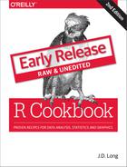
x <- 10
y <- 50
z <- c("three", "blind", "mice")
f <- function(n, p) sqrt(p * (1 - p) / n)
ls()
#> [1] "f" "x" "y" "z"

Notice that ls returns a vector of character strings in which each string is the name of one variable or function. When your workspace is empty, ls returns an empty vector, which produces this puzzling output:

ls()
#> character(0)

That is R’s quaint way of saying that ls returned a zero-length vector of strings; that is, it returned an empty vector because nothing is defined in your workspace.

If you want more than just a list of names, try ls.str; this will also tell you something about each variable:

x <- 10
y <- 50
z <- c("three", "blind", "mice")
f <- function(n, p) sqrt(p * (1 - p) / n)
ls.str()
#> f : function (n, p)
#> x :  num 10
#> y :  num 50
#> z :  chr [1:3] "three" "blind" "mice"

The function is called ls.str because it is both listing your variables and applying the str function to them, showing their structure (Revealing the Structure of an Object).

Ordinarily, ls does not return any name that begins with a dot (.). Such names are considered hidden and are not normally of interest to users. (This mirrors the Unix convention of not listing files whose names begin with dot.) You can force ls to list everything by setting the all.names argument to TRUE:

ls()
#> [1] "f" "x" "y" "z"
ls(all.names = TRUE)
#> [1] ".Random.seed" "f"            "x"            "y"
#> [5] "z"

See Also

See “Deleting Variables” for deleting variables and Recipe X-X for inspecting your variables.

Problem

You want to remove unneeded variables or functions from your workspace or to erase its contents completely.

Solution

Use the rm function.

Discussion

Your workspace can get cluttered quickly. The rm function removes, permanently, one or more objects from the workspace:

x <- 2 * pi
x
#> [1] 6.28
rm(x)
x
#> Error in eval(expr, envir, enclos): object 'x' not found

There is no “undo”; once the variable is gone, it’s gone.

You can remove several variables at once:

rm(x, y, z)

You can even erase your entire workspace at once. The rm function has a list argument consisting of a vector of names of variables to remove. Recall that the ls function returns a vector of variables names; hence you can combine rm and ls to erase everything:

ls()
#> [1] "f" "x" "y" "z"
rm(list = ls())
ls()
#> character(0)

Alternativly you could click the broom icon in the top of the Environment pane in R Studio, shown in Figure 2-1.

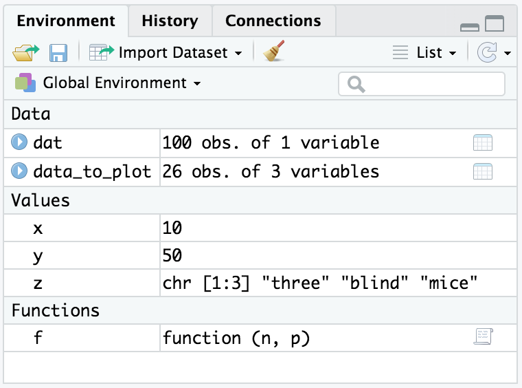
Figure 2-1. Environment Panel in R Studio

Never put rm(list=ls()) into code you share with others, such as a library function or sample code sent to a mailing list or Stack Overflow. Deleting all the variables in someone else’s workspace is worse than rude and will make you extremely unpopular.

See Also

See “Listing Variables”.

Problem

You want to create a vector.

Solution

Use the c(...) operator to construct a vector from given values.

Discussion

Vectors are a central component of R, not just another data structure. A vector can contain either numbers, strings, or logical values but not a mixture.

The c(...) operator can construct a vector from simple elements:

c(1, 1, 2, 3, 5, 8, 13, 21)
#> [1]  1  1  2  3  5  8 13 21
c(1 * pi, 2 * pi, 3 * pi, 4 * pi)
#> [1]  3.14  6.28  9.42 12.57
c("My", "twitter", "handle", "is", "@cmastication")
#> [1] "My"            "twitter"       "handle"        "is"
#> [5] "@cmastication"
c(TRUE, TRUE, FALSE, TRUE)
#> [1]  TRUE  TRUE FALSE  TRUE

If the arguments to c(...) are themselves vectors, it flattens them and combines them into one single vector:

v1 <- c(1, 2, 3)
v2 <- c(4, 5, 6)
c(v1, v2)
#> [1] 1 2 3 4 5 6

Vectors cannot contain a mix of data types, such as numbers and strings. If you create a vector from mixed elements, R will try to accommodate you by converting one of them:

v1 <- c(1, 2, 3)
v3 <- c("A", "B", "C")
c(v1, v3)
#> [1] "1" "2" "3" "A" "B" "C"

Here, the user tried to create a vector from both numbers and strings. R converted all the numbers to strings before creating the vector, thereby making the data elements compatible. Note that R does this without warning or complaint.

Technically speaking, two data elements can coexist in a vector only if they have the same mode. The modes of 3.1415 and "foo" are numeric and character, respectively:

mode(3.1415)
#> [1] "numeric"
mode("foo")
#> [1] "character"

Those modes are incompatible. To make a vector from them, R converts 3.1415 to character mode so it will be compatible with "foo":

c(3.1415, "foo")
#> [1] "3.1415" "foo"
mode(c(3.1415, "foo"))
#> [1] "character"

See Also

See the “Introduction” to the Chapter 5 chapter for more about vectors and other data structures.

Problem

You want to calculate basic statistics: mean, median, standard deviation, variance, correlation, or covariance.

Solution

Use one of these functions as applies, assuming that x and y are vectors:

• mean(x)

• median(x)

• sd(x)

• var(x)

• cor(x, y)

• cov(x, y)

Discussion

When you first use R you might open the docuentation and begin searching for material entitled “Procedures for Calculating Standard Deviation.” It seems that such an important topic would likely require a whole chapter.

It’s not that complicated.

Standard deviation and other basic statistics are calculated by simple functions. Ordinarily, the function argument is a vector of numbers and the function returns the calculated statistic:

x <- c(0, 1, 1, 2, 3, 5, 8, 13, 21, 34)
mean(x)
#> [1] 8.8
median(x)
#> [1] 4
sd(x)
#> [1] 11
var(x)
#> [1] 122

The sd function calculates the sample standard deviation, and var calculates the sample variance.

The cor and cov functions can calculate the correlation and covariance, respectively, between two vectors:

x <- c(0, 1, 1, 2, 3, 5, 8, 13, 21, 34)
y <- log(x + 1)
cor(x, y)
#> [1] 0.907
cov(x, y)
#> [1] 11.5

All these functions are picky about values that are not available (NA). Even one NA value in the vector argument causes any of these functions to return NA or even halt altogether with a cryptic error:

x <- c(0, 1, 1, 2, 3, NA)
mean(x)
#> [1] NA
sd(x)
#> [1] NA

It’s annoying when R is that cautious, but it is the right thing to do. You must think carefully about your situation. Does an NA in your data invalidate the statistic? If yes, then R is doing the right thing. If not, you can override this behavior by setting na.rm=TRUE, which tells R to ignore the NA values:

x <- c(0, 1, 1, 2, 3, NA)
sd(x, na.rm = TRUE)
#> [1] 1.14

In older versions of R, mean and sd were smart about data frames. They understood that each column of the data frame is a different variable, so they calculated their statistic for each column individually. This is no longer the case and, as a result, you may read confusing comments online or in older books (like version 1 of this book). In order to apply the functions to each column of a dataframe we now need to use a helper function. The Tidyverse family of helper functions for this sort of thing are in the purrr package. As with other Tidyverse packages, this gets loaded when you run library(tidyverse). The function we’ll use to apply a function to each column of a data frame is map_dbl:

data(cars)

map_dbl(cars, mean)
#> speed  dist
#>  15.4  43.0
map_dbl(cars, sd)
#> speed  dist
#>  5.29 25.77
map_dbl(cars, median)
#> speed  dist
#>    15    36

Notice that using map_dbl to apply mean or sd each return two values, one for each column defined by the data frame. (Technically, they return a two-element vector whose names attribute is taken from the columns of the data frame.)

The var function understands data frames without the help of a mapping function. It calculates the covariance between the columns of the data frame and returns the covariance matrix:

var(cars)
#>       speed dist
#> speed    28  110
#> dist    110  664

Likewise, if x is either a data frame or a matrix, then cor(x) returns the correlation matrix and cov(x) returns the covariance matrix:

cor(cars)
#>       speed  dist
#> speed 1.000 0.807
#> dist  0.807 1.000
cov(cars)
#>       speed dist
#> speed    28  110
#> dist    110  664

See Also

See Recipes:
“Avoiding Some Common Mistakes”

“Merging Data Frames by Common Column”

Recipe X-X

Problem

You want to create a sequence of numbers.

Solution

Use an n:m expression to create the simple sequence n, n+1, n+2, …, m:

1:5
#> [1] 1 2 3 4 5

Use the seq function for sequences with an increment other than 1:

seq(from = 1, to = 5, by = 2)
#> [1] 1 3 5

Use the rep function to create a series of repeated values:

rep(1, times = 5)
#> [1] 1 1 1 1 1

Discussion

The colon operator (n:m) creates a vector containing the sequence n, n+1, n+2, …, m:

0:9
#>  [1] 0 1 2 3 4 5 6 7 8 9
10:19
#>  [1] 10 11 12 13 14 15 16 17 18 19
9:0
#>  [1] 9 8 7 6 5 4 3 2 1 0

Observe that R was clever with the last expression (9:0). Because 9 is larger than 0, it counts backward from the starting to ending value. You can also use the colon operator directly with the pipe to pass data to another function:

10:20 %>% mean()

The colon operator works for sequences that grow by 1 only. The seq function also builds sequences but supports an optional third argument, which is the increment:

seq(from = 0, to = 20)
#>  [1]  0  1  2  3  4  5  6  7  8  9 10 11 12 13 14 15 16 17 18 19 20
seq(from = 0, to = 20, by = 2)
#>  [1]  0  2  4  6  8 10 12 14 16 18 20
seq(from = 0, to = 20, by = 5)
#> [1]  0  5 10 15 20

Alternatively, you can specify a length for the output sequence and then R will calculate the necessary increment:

seq(from = 0, to = 20, length.out = 5)
#> [1]  0  5 10 15 20
seq(from = 0, to = 100, length.out = 5)
#> [1]   0  25  50  75 100

The increment need not be an integer. R can create sequences with fractional increments, too:

seq(from = 1.0, to = 2.0, length.out = 5)
#> [1] 1.00 1.25 1.50 1.75 2.00

For the special case of a “sequence” that is simply a repeated value you should use the rep function, which repeats its first argument:

rep(pi, times = 5)
#> [1] 3.14 3.14 3.14 3.14 3.14

See Also

See “Creating a Sequence of Dates” for creating a sequence of Date objects.

Problem

You want to compare two vectors or you want to compare an entire vector against a scalar.

Solution

The comparison operators (==, !=, <, >, <=, >=) can perform an element-by-element comparison of two vectors. They can also compare a vector’s element against a scalar. The result is a vector of logical values in which each value is the result of one element-wise comparison.

Discussion

R has two logical values, TRUE and FALSE. These are often called Boolean values in other programming languages.

The comparison operators compare two values and return TRUE or FALSE, depending upon the result of the comparison:

a <- 3
a == pi # Test for equality
#> [1] FALSE
a != pi # Test for inequality
#> [1] TRUE
a < pi
#> [1] TRUE
a > pi
#> [1] FALSE
a <= pi
#> [1] TRUE
a >= pi
#> [1] FALSE

You can experience the power of R by comparing entire vectors at once. R will perform an element-by-element comparison and return a vector of logical values, one for each comparison:

v <- c(3, pi, 4)
w <- c(pi, pi, pi)
v == w # Compare two 3-element vectors
#> [1] FALSE  TRUE FALSE
v != w
#> [1]  TRUE FALSE  TRUE
v < w
#> [1]  TRUE FALSE FALSE
v <= w
#> [1]  TRUE  TRUE FALSE
v > w
#> [1] FALSE FALSE  TRUE
v >= w
#> [1] FALSE  TRUE  TRUE

You can also compare a vector against a single scalar, in which case R will expand the scalar to the vector’s length and then perform the element-wise comparison. The previous example can be simplified in this way:

v <- c(3, pi, 4)
v == pi # Compare a 3-element vector against one number
#> [1] FALSE  TRUE FALSE
v != pi
#> [1]  TRUE FALSE  TRUE

(This is an application of the Recycling Rule, “Understanding the Recycling Rule”.)

After comparing two vectors, you often want to know whether any of the comparisons were true or whether all the comparisons were true. The any and all functions handle those tests. They both test a logical vector. The any function returns TRUE if any element of the vector is TRUE. The all function returns TRUE if all elements of the vector are TRUE:

v <- c(3, pi, 4)
any(v == pi) # Return TRUE if any element of v equals pi
#> [1] TRUE
all(v == 0) # Return TRUE if all elements of v are zero
#> [1] FALSE

See Also

See “Selecting Vector Elements”.

Problem

You want to extract one or more elements from a vector.

Solution

Select the indexing technique appropriate for your problem:

• Use square brackets to select vector elements by their position, such as v[3] for the third element of v.

• Use negative indexes to exclude elements.

• Use a vector of indexes to select multiple values.

• Use a logical vector to select elements based on a condition.

• Use names to access named elements.

Discussion

Selecting elements from vectors is another powerful feature of R. Basic selection is handled just as in many other programming languages—use square brackets and a simple index:

fib <- c(0, 1, 1, 2, 3, 5, 8, 13, 21, 34)
fib
#>  [1]  0  1  1  2  3  5  8 13 21 34
fib[1]
#> [1] 0
fib[2]
#> [1] 1
fib[3]
#> [1] 1
fib[4]
#> [1] 2
fib[5]
#> [1] 3

Notice that the first element has an index of 1, not 0 as in some other programming languages.

A cool feature of vector indexing is that you can select multiple elements at once. The index itself can be a vector, and each element of that indexing vector selects an element from the data vector:

fib[1:3] # Select elements 1 through 3
#> [1] 0 1 1
fib[4:9] # Select elements 4 through 9
#> [1]  2  3  5  8 13 21

An index of 1:3 means select elements 1, 2, and 3, as just shown. The indexing vector needn’t be a simple sequence, however. You can select elements anywhere within the data vector—as in this example, which selects elements 1, 2, 4, and 8:

fib[c(1, 2, 4, 8)]
#> [1]  0  1  2 13

R interprets negative indexes to mean exclude a value. An index of −1, for instance, means exclude the first value and return all other values:

fib[-1] # Ignore first element
#> [1]  1  1  2  3  5  8 13 21 34

This method can be extended to exclude whole slices by using an indexing vector of negative indexes:

fib[1:3] # As before
#> [1] 0 1 1
fib[-(1:3)] # Invert sign of index to exclude instead of select
#> [1]  2  3  5  8 13 21 34

Another indexing technique uses a logical vector to select elements from the data vector. Everywhere that the logical vector is TRUE, an element is selected:

fib < 10 # This vector is TRUE wherever fib is less than 10
#>  [1]  TRUE  TRUE  TRUE  TRUE  TRUE  TRUE  TRUE FALSE FALSE FALSE
fib[fib < 10] # Use that vector to select elements less than 10
#> [1] 0 1 1 2 3 5 8
fib %% 2 == 0 # This vector is TRUE wherever fib is even
#>  [1]  TRUE FALSE FALSE  TRUE FALSE FALSE  TRUE FALSE FALSE  TRUE
fib[fib %% 2 == 0] # Use that vector to select the even elements
#> [1]  0  2  8 34

Ordinarily, the logical vector should be the same length as the data vector so you are clearly either including or excluding each element. (If the lengths differ then you need to understand the Recycling Rule, “Understanding the Recycling Rule”.)

By combining vector comparisons, logical operators, and vector indexing, you can perform powerful selections with very little R code:

Select all elements greater than the median

v <- c(3, 6, 1, 9, 11, 16, 0, 3, 1, 45, 2, 8, 9, 6, -4)
v[ v > median(v)]
#> [1]  9 11 16 45  8  9

Select all elements in the lower and upper 5%

v[ (v < quantile(v, 0.05)) | (v > quantile(v, 0.95)) ]
#> [1] 45 -4

The above example uses the | operator which means “or” when indexing. If you wanted “and” you use the & operator.

Select all elements that exceed ±1 standard deviations from the mean

v[ abs(v - mean(v)) > sd(v)]
#> [1] 45 -4

Select all elements that are neither NA nor NULL

v <- c(1, 2, 3, NA, 5)
v[!is.na(v) & !is.null(v)]
#> [1] 1 2 3 5

One final indexing feature lets you select elements by name. It assumes that the vector has a names attribute, defining a name for each element. This can be done by assigning a vector of character strings to the attribute:

years <- c(1960, 1964, 1976, 1994)
names(years) <- c("Kennedy", "Johnson", "Carter", "Clinton")
years
#> Kennedy Johnson  Carter Clinton
#>    1960    1964    1976    1994

Once the names are defined, you can refer to individual elements by name:

years["Carter"]
#> Carter
#>   1976
years["Clinton"]
#> Clinton
#>    1994

This generalizes to allow indexing by vectors of names: R returns every element named in the index:

years[c("Carter", "Clinton")]
#>  Carter Clinton
#>    1976    1994

See Also

See “Understanding the Recycling Rule” for more about the Recycling Rule.

Problem

You want to operate on an entire vector at once.

Solution

The usual arithmetic operators can perform element-wise operations on entire vectors. Many functions operate on entire vectors, too, and return a vector result.

Discussion

Vector operations are one of R’s great strengths. All the basic arithmetic operators can be applied to pairs of vectors. They operate in an element-wise manner; that is, the operator is applied to corresponding elements from both vectors:

v <- c(11, 12, 13, 14, 15)
w <- c(1, 2, 3, 4, 5)
v + w
#> [1] 12 14 16 18 20
v - w
#> [1] 10 10 10 10 10
v * w
#> [1] 11 24 39 56 75
v / w
#> [1] 11.00  6.00  4.33  3.50  3.00
w^v
#> [1] 1.00e+00 4.10e+03 1.59e+06 2.68e+08 3.05e+10

Observe that the length of the result here is equal to the length of the original vectors. The reason is that each element comes from a pair of corresponding values in the input vectors.

If one operand is a vector and the other is a scalar, then the operation is performed between every vector element and the scalar:

w
#> [1] 1 2 3 4 5
w + 2
#> [1] 3 4 5 6 7
w - 2
#> [1] -1  0  1  2  3
w * 2
#> [1]  2  4  6  8 10
w / 2
#> [1] 0.5 1.0 1.5 2.0 2.5
2^w
#> [1]  2  4  8 16 32

For example, you can recenter an entire vector in one expression simply by subtracting the mean of its contents:

w
#> [1] 1 2 3 4 5
mean(w)
#> [1] 3
w - mean(w)
#> [1] -2 -1  0  1  2

Likewise, you can calculate the z-score of a vector in one expression: subtract the mean and divide by the standard deviation:

w
#> [1] 1 2 3 4 5
sd(w)
#> [1] 1.58
(w - mean(w)) / sd(w)
#> [1] -1.265 -0.632  0.000  0.632  1.265

Yet the implementation of vector-level operations goes far beyond elementary arithmetic. It pervades the language, and many functions operate on entire vectors. The functions sqrt and log, for example, apply themselves to every element of a vector and return a vector of results:

w <- 1:5
w
#> [1] 1 2 3 4 5
sqrt(w)
#> [1] 1.00 1.41 1.73 2.00 2.24
log(w)
#> [1] 0.000 0.693 1.099 1.386 1.609
sin(w)
#> [1]  0.841  0.909  0.141 -0.757 -0.959

There are two great advantages to vector operations. The first and most obvious is convenience. Operations that require looping in other languages are one-liners in R. The second is speed. Most vectorized operations are implemented directly in C code, so they are substantially faster than the equivalent R code you could write.

See Also

Performing an operation between a vector and a scalar is actually a special case of the Recycling Rule; see “Understanding the Recycling Rule”.

Problem

Your R expression is producing a curious result, and you wonder if operator precedence is causing problems.

Solution

The full list of operators is shown in table @ref(tab:precedence), listed in order of precedence from highest to lowest. Operators of equal precedence are evaluated from left to right except where indicated.

It’s not important that you know what every one of these operators do, or what they mean. The list here is to expose you to the idea that different operators have different precedence.

Discussion

Getting your operator precedence wrong in R is a common problem. It certainly happens to the authors a lot. We unthinkingly expect that the expression 0:n−1 will create a sequence of integers from 0 to n − 1 but it does not:

n <- 10
0:n - 1
#>  [1] -1  0  1  2  3  4  5  6  7  8  9

It creates the sequence from −1 to n − 1 because R interprets it as (0:n)−1.

You might not recognize the notation %`_any_%` in the table. R interprets any text between percent signs (%…%) as a binary operator. Several such operators have predefined meanings:

%%

Modulo operator

%/%

Integer division

%*%

Matrix multiplication

%in%

Returns TRUE if the left operand occurs in its right operand; FALSE otherwise

%>%

Pipe that passes results from the left to a function on the right

You can also define new binary operators using the %…% notation; see Defining Your Own Binary Operators. The point here is that all such operators have the same precedence.

See Also

See “Performing Vector Arithmetic” for more about vector operations, “Performing Matrix Operations” for more about matrix operations, and Recipe X-X to define your own operators. See the Arithmetic and Syntax topics in the R help pages as well as Chapters 5 and 6 of R in a Nutshell (O’Reilly).

Problem

You are getting tired of typing long sequences of commands and especially tired of typing the same ones over and over.

Solution

Open an editor window and accumulate your reusable blocks of R commands there. Then, execute those blocks directly from that window. Reserve the command line for typing brief or one-off commands.

When you are done, you can save the accumulated code blocks in a script file for later use.

Discussion

The typical beginner to R types an expression in the console window and sees what happens. As he gets more comfortable, he types increasingly complicated expressions. Then he begins typing multiline expressions. Soon, he is typing the same multiline expressions over and over, perhaps with small variations, in order to perform his increasingly complicated calculations.

The experienced user does not often retype a complex expression. She may type the same expression once or twice, but when she realizes it is useful and reusable she will cut-and-paste it into an editor window. To execute the snippet thereafter, she selects the snippet in the editor window and tells R to execute it, rather than retyping it. This technique is especially powerful as her snippets evolve into long blocks of code.

In R Studio, a few features of the IDE facilitate this workstyle. Windows and Linux machines have slightly different keys than Mac machines: Windows/Linux uses the Ctrl and Alt modifiers, whereas the Mac uses Cmd and Opt.

To open an editor window

From the main menu, select File → New File then select the type of file you want to create, in this case, an R Script.

To execute one line of the editor window

Position the cursor on the line and then press Ctrl+Enter (Windows) or Cmd+Enter (Mac) to execute it.

To execute several lines of the editor window

Highlight the lines using your mouse; then press Ctrl+Enter (Windows) or Cmd+Enter (Mac) to execute them.

To execute the entire contents of the editor window

Press Ctrl+Alt+R (Windows) or Cmd+Opt+R (Mac) to execute the whole editor window. Or from the menu click Code → Run Region → Run All

These keyboard shortcuts and dozens more can be found within R Studio by clicking the menu: Tools → Keyboard Shortcuts Help

Copying lines from the console window to the editor window is simply a matter of copy and paste. When you exit R Studio, it will ask if you want to save the new script. You can either save it for future reuse or discard it.

Problem

Creating many intermediate variables in your code is tedious and overly verbose, while nesting R functions seems nearly unreadable.

Solution

Use the pipe operator (%>%) to make your expression easier to read and write. The pipe operator (%>%), created by Stefan Bache and found in the magrittr package and used extensivly in many tidyverse functions as well.

Us the pipe operator to combine multiple functions together into a “pipeline” of functions without intermediate variables:

library(tidyverse)
data(mpg)

mpg %>%
  filter(cty > 21) %>%
  head(3) %>%
  print()
#> # A tibble: 3 x 11
#>   manufacturer model displ  year   cyl trans drv     cty   hwy fl    class
#>   <chr>        <chr> <dbl> <int> <int> <chr> <chr> <int> <int> <chr> <chr>
#> 1 chevrolet    mali~   2.4  2008     4 auto~ f        22    30 r     mids~
#> 2 honda        civic   1.6  1999     4 manu~ f        28    33 r     subc~
#> 3 honda        civic   1.6  1999     4 auto~ f        24    32 r     subc~

The pipe is much cleaner and easier to read than using intermediate temporary variables:

temp1 <- filter(mpg, cty > 21)
temp2 <- head(temp1, 3)
print(temp2)
#> # A tibble: 3 x 11
#>   manufacturer model displ  year   cyl trans drv     cty   hwy fl    class
#>   <chr>        <chr> <dbl> <int> <int> <chr> <chr> <int> <int> <chr> <chr>
#> 1 chevrolet    mali~   2.4  2008     4 auto~ f        22    30 r     mids~
#> 2 honda        civic   1.6  1999     4 manu~ f        28    33 r     subc~
#> 3 honda        civic   1.6  1999     4 auto~ f        24    32 r     subc~

Discussion

The pipe operator does not provide any new functionality to R, but it can greatly improve readability of code. The pipe operator takes the output of the function or object on the left of the operator and passes it as the first argument of the function on the right.

Writing this:

x %>% head()

is functionally the same as writing this:

head(x)

In both cases x is the argument to head. We can supply additional arguments, but x is always the first argument. These two lines are functionally identical:

x %>% head(n = 10)

head(x, n = 10)

This difference may seem small, but with a more complicated example, the benefits begin to accumulate. If we had a workflow where we wanted to use filter to limit our data to values, then select to keep only certain variables, followed by ggplot to create a simple plot, we could use intermediate variables.

library(tidyverse)

filtered_mpg <- filter(mpg, cty > 21)
selected_mpg <- select(filtered_mpg, cty, hwy)
ggplot(selected_mpg, aes(cty, hwy)) + geom_point()

This incremental approach is fairly readable but creates a number of intermediate data frames and requires the user to keep track of the state of many objects which can generate a cognitive load on the user.

Another alternative is to nest the functions together:

ggplot(select(filter(mpg, cty > 21), cty, hwy), aes(cty, hwy)) + geom_point()

While this is very concise since it’s only one line, this code requires much more attention to read and understand what’s going on. Code that is difficult for the user to parse mentally can introduce potential for error, and also make maintenance of the code harder in the future.

mpg %>%
  filter(cty > 21) %>%
  select(cty, hwy) %>%
  ggplot(aes(cty, hwy)) + geom_point()

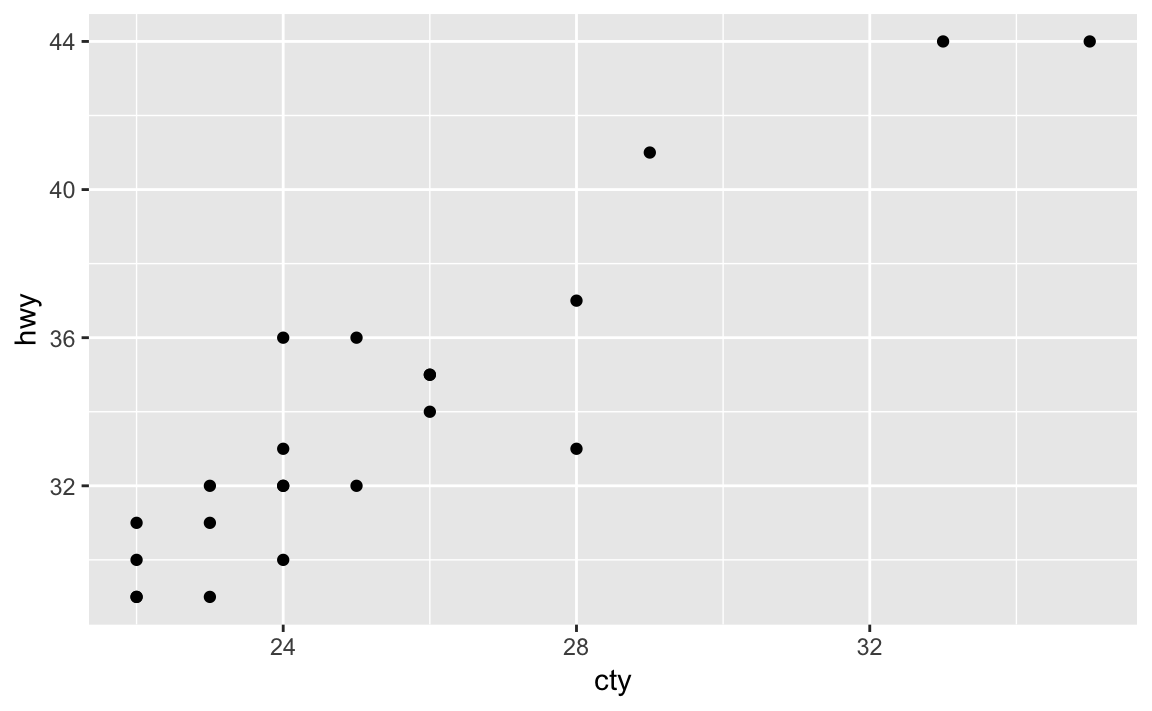
Figure 2-2. Plotting with pipes example

The above code starts with the mpg dataset, pipes it to the filter function which keeps only records where the city mpg (cty) is greater than 21. Those results are piped into the select command that keeps only the listed variables cty and hwy and those are piped into the ggplot command where an point plot is produced in Figure 2-2

If you want the argument going into your target (right hand side) function to be somewhere other than the first argument, use the dot (.) operator:

iris %>% head(3)

is the same as:

iris %>% head(3, x = .)

However in the second example we passed the iris data frame into the second named argument using the dot operator. This can be handy for functions where the input data frame goes in a position other than the first argument.

Through this book we use pipes to hold together data transformations with multiple steps. We typically format the code with a line break after each pipe and then we indent the code on the following lines. This makes the code easily identifiable as parts of the same data pipeline.

Problem

You want to avoid some of the common mistakes made by beginning users—and also by experienced users, for that matter.

Discussion

Here are some easy ways to make trouble for yourself:

Forgetting the parentheses after a function invocation:
You call an R function by putting parentheses after the name. For instance, this line invokes the ls function:

ls()

However, if you omit the parentheses then R does not execute the function. Instead, it shows the function definition, which is almost never what you want:

ls

# > function (name, pos = -1L, envir = as.environment(pos), all.names = FALSE,
# >     pattern, sorted = TRUE)
# > {
# >     if (!missing(name)) {
# >         pos <- tryCatch(name, error = function(e) e)
# >         if (inherits(pos, "error")) {
# >             name <- substitute(name)
# >             if (!is.character(name))
# >                 name <- deparse(name)
# > etc...

Forgetting to double up backslashes in Windows file paths
This function call appears to read a Windows file called F:\research\bio\assay.csv, but it does not:

tbl <- read.csv("F:\research\bio\assay.csv")

Backslashes (\) inside character strings have a special meaning and therefore need to be doubled up. R will interpret this file name as F:researchbioassay.csv, for example, which is not what the user wanted. See “Dealing with “Cannot Open File” in Windows” for possible solutions.

Mistyping “<-” as “< (blank) -”
The assignment operator is <-, with no space between the < and the -:

x <- pi # Set x to 3.1415926...

If you accidentally insert a space between < and -, the meaning changes completely:

x < -pi # Oops! We are comparing x instead of setting it!
#> [1] FALSE

This is now a comparison (<) between x and negative π (-pi). It does not change x. If you are lucky, x is undefined and R will complain, alerting you that something is fishy:

x < -pi
#> Error in eval(expr, envir, enclos): object 'x' not found

If x is defined, R will perform the comparison and print a logical value, TRUE or FALSE. That should alert you that something is wrong: an assignment does not normally print anything:

x <- 0 # Initialize x to zero
x < -pi # Oops!
#> [1] FALSE

Incorrectly continuing an expression across lines
R reads your typing until you finish a complete expression, no matter how many lines of input that requires. It prompts you for additional input using the + prompt until it is satisfied. This example splits an expression across two lines:

total <- 1 + 2 + 3 + # Continued on the next line
  4 + 5
print(total)
#> [1] 15

Problems begin when you accidentally finish the expression prematurely, which can easily happen:

total <- 1 + 2 + 3 # Oops! R sees a complete expression
+4 + 5 # This is a new expression; R prints its value
#> [1] 9
print(total)
#> [1] 6

There are two clues that something is amiss: R prompted you with a normal prompt (>), not the continuation prompt (+); and it printed the value of 4 + 5.

This common mistake is a headache for the casual user. It is a nightmare for programmers, however, because it can introduce hard-to-find bugs into R scripts.

Using = instead of ==
Use the double-equal operator (==) for comparisons. If you accidentally use the single-equal operator (=), you will irreversibly overwrite your variable:

v <- 1 # Assign 1 to v
v == 0 # Compare v against zero
#> [1] FALSE
v <- 0 # Assign 0 to v, overwriting previous contents

Writing 1:n+1 when you mean 1:(n+1)
You might think that 1:n+1 is the sequence of numbers 1, 2, …, n, n + 1. It’s not. It is the sequence 1, 2, …, n with 1 added to every element, giving 2, 3, …, n, n + 1. This happens because R interprets 1:n+1 as (1:n)+1. Use parentheses to get exactly what you want:

n <- 5
1:n + 1
#> [1] 2 3 4 5 6
1:(n + 1)
#> [1] 1 2 3 4 5 6

Getting bitten by the Recycling Rule
Vector arithmetic and vector comparisons work well when both vectors have the same length. However, the results can be baffling when the operands are vectors of differing lengths. Guard against this possibility by understanding and remembering the Recycling Rule, “Understanding the Recycling Rule”.

Installing a package but not loading it with library() or require()
Installing a package is the first step toward using it, but one more step is required. Use library or require to load the package into your search path. Until you do so, R will not recognize the functions or datasets in the package. See “Accessing the Functions in a Package”:

x <- rnorm(100)
n <- 5
truehist(x, n)
#> Error in truehist(x, n): could not find function "truehist"

However if we load the library first, then the code runs and we get the chart shown in Figure 2-3.

library(MASS) # Load the MASS package into R
truehist(x, n)

Figure 2-3. Example truehist

We typically use library() instead of require(). The reason is that if you create an R script that uses library() and the desired package is not already installed, R will return an error. While require(), in contrast, will simply return FALSE if the package is not installed.

Writing aList[i] when you mean aList[[i]], or vice versa
If the variable lst contains a list, it can be indexed in two ways: lst[[n]] is the _n_th element of the list; whereas lst[n] is a list whose only element is the _n_th element of lst. That’s a big difference. See “Selecting List Elements by Position”.

Using & instead of &&, or vice versa; same for | and ||
Use & and | in logical expressions involving the logical values TRUE and FALSE. See “Selecting Vector Elements”.

Use && and || for the flow-of-control expressions inside if and while statements.

Programmers accustomed to other programming languages may reflexively use && and || everywhere because “they are faster.” But those operators give peculiar results when applied to vectors of logical values, so avoid them unless you are sure that they do what you want.

Passing multiple arguments to a single-argument function
What do you think is the value of mean(9,10,11)? No, it’s not 10. It’s 9. The mean function computes the mean of the first argument. The second and third arguments are being interpreted as other, positional arguments. To pass multiple items into a single argument, we put them in a vector with the c operator. mean(c(9,10,11)) will return 10, as you might expect.

Some functions, such as mean, take one argument. Other arguments, such as max and min, take multiple arguments and apply themselves across all arguments. Be sure you know which is which.

Thinking that max behaves like pmax, or that min behaves like pmin
The max and min functions have multiple arguments and return one value: the maximum or minimum of all their arguments.

The pmax and pmin functions have multiple arguments but return a vector with values taken element-wise from the arguments. See Finding Parwise Minimums or Maximums.

Misusing a function that does not understand data frames
Some functions are quite clever regarding data frames. They apply themselves to the individual columns of the data frame, computing their result for each individual column. Sadly, not all functions are that clever. This includes the mean, median, max, and min functions. They will lump together every value from every column and compute their result from the lump or possibly just return an error. Be aware of which functions are savvy to data frames and which are not.

Using single backslash (\) in Windows Paths If you are using R on Windows, it is common to copy and paste a file path into your R script. Windows File Explorer will show you that your path is C:\temp\my_file.csv but if you try to tell R to read that file, you’ll get a cryptic message:

Error: '\m' is an unrecognized escape in character string starting "'.\temp\m"

This is because R sees backslashes as special characters. You can get around this either by using forward slashes (/), or using double backslashes, (\\).

read_csv(`./temp/my_file.csv`)
read_csv(`.\\temp\\my_file.csv`)

This is only an issue on Windows because both Mac and Linux use forward slashes as path seperators.

Posting a question to Stack Overflow or the mailing list before searching for the answer
Don’t waste your time. Don’t waste other people’s time. Before you post a question to a mailing list or to Stack Overflow, do your homework and search the archives. Odds are, someone has already answered your question. If so, you’ll see the answer in the discussion thread for the question. See “Searching the Mailing Lists”.

See Also

See Recipes , , , and .