Table of Contents for
Python for Data Analysis, 2nd Edition
 Python for Data Analysis, 2nd Edition
Published by
O'Reilly Media, Inc., 2017
Python for Data Analysis, 2nd Edition
Published by
O'Reilly Media, Inc., 2017
- nav
- Cover
- Python for Data Analysis
- Python for Data Analysis
- Preface
- Preliminaries
- Python Language Basics, IPython, and Jupyter Notebooks
- Built-in Data Structures, Functions, and Files
- NumPy Basics: Arrays and Vectorized Computation
- Getting Started with pandas
- Data Loading, Storage, and File Formats
- Data Cleaning and Preparation
- Data Wrangling: Join, Combine, and Reshape
- Plotting and Visualization
- Data Aggregation and Group Operations
- Time Series
- Advanced pandas
- Introduction to Modeling Libraries in Python
- Data Analysis Examples
- Advanced NumPy
- More on the IPython System
- Index
- About the Author
- Colophon
Chapter 11. Time Series
Time series data is an important form of structured data in many different fields, such as finance, economics, ecology, neuroscience, and physics. Anything that is observed or measured at many points in time forms a time series. Many time series are fixed frequency, which is to say that data points occur at regular intervals according to some rule, such as every 15 seconds, every 5 minutes, or once per month. Time series can also be irregular without a fixed unit of time or offset between units. How you mark and refer to time series data depends on the application, and you may have one of the following:
Fixed periods, such as the month January 2007 or the full year 2010
Intervals of time, indicated by a start and end timestamp. Periods can be thought of as special cases of intervals
Experiment or elapsed time; each timestamp is a measure of time relative to a particular start time (e.g., the diameter of a cookie baking each second since being placed in the oven)
In this chapter, I am mainly concerned with time series in the first three categories, though many of the techniques can be applied to experimental time series where the index may be an integer or floating-point number indicating elapsed time from the start of the experiment. The simplest and most widely used kind of time series are those indexed by timestamp.
Tip
pandas also supports indexes based on timedeltas, which can be a useful way of representing experiment or elapsed time. We do not explore timedelta indexes in this book, but you can learn more in the pandas documentation.
pandas provides many built-in time series tools and data algorithms. You can efficiently work with very large time series and easily slice and dice, aggregate, and resample irregular- and fixed-frequency time series. Some of these tools are especially useful for financial and economics applications, but you could certainly use them to analyze server log data, too.
11.1 Date and Time Data Types and Tools
The Python standard library includes data types for date and time data, as well
as calendar-related functionality. The datetime, time, and calendar modules are the main places to start. The datetime.datetime type, or simply datetime, is widely used:
In[10]:fromdatetimeimportdatetimeIn[11]:now=datetime.now()In[12]:nowOut[12]:datetime.datetime(2017,10,17,13,34,33,597499)In[13]:now.year,now.month,now.dayOut[13]:(2017,10,17)
datetime stores both the
date and time down to the microsecond. timedelta represents the temporal difference
between two datetime objects:
In[14]:delta=datetime(2011,1,7)-datetime(2008,6,24,8,15)In[15]:deltaOut[15]:datetime.timedelta(926,56700)In[16]:delta.daysOut[16]:926In[17]:delta.secondsOut[17]:56700
You can add (or subtract) a timedelta or multiple thereof to a datetime object to yield a new shifted
object:
In[18]:fromdatetimeimporttimedeltaIn[19]:start=datetime(2011,1,7)In[20]:start+timedelta(12)Out[20]:datetime.datetime(2011,1,19,0,0)In[21]:start-2*timedelta(12)Out[21]:datetime.datetime(2010,12,14,0,0)
Table 11-1 summarizes the data types
in the datetime module. While this
chapter is mainly concerned with the data types in pandas and higher-level
time series manipulation, you may encounter the datetime-based types in many other places in
Python in the wild.
Converting Between String and Datetime
You can format datetime objects and pandas Timestamp
objects, which I’ll introduce later, as strings
using str or the
strftime method, passing a format
specification:
In[22]:stamp=datetime(2011,1,3)In[23]:str(stamp)Out[23]:'2011-01-03 00:00:00'In[24]:stamp.strftime('%Y-%m-%d')Out[24]:'2011-01-03'
See Table 11-2 for a complete list of the format codes (reproduced from Chapter 2).
You can use these same format codes to convert strings to dates
using datetime.strptime:
In[25]:value='2011-01-03'In[26]:datetime.strptime(value,'%Y-%m-%d')Out[26]:datetime.datetime(2011,1,3,0,0)In[27]:datestrs=['7/6/2011','8/6/2011']In[28]:[datetime.strptime(x,'%m/%d/%Y')forxindatestrs]Out[28]:[datetime.datetime(2011,7,6,0,0),datetime.datetime(2011,8,6,0,0)]
datetime.strptime is a good way
to parse a date with a known format. However, it can be a bit annoying
to have to write a format spec each time, especially for common date
formats. In this case, you can use the parser.parse method in the third-party dateutil
package (this is installed automatically when you install pandas):
In[29]:fromdateutil.parserimportparseIn[30]:parse('2011-01-03')Out[30]:datetime.datetime(2011,1,3,0,0)
dateutil is capable of parsing
most human-intelligible date representations:
In[31]:parse('Jan 31, 1997 10:45 PM')Out[31]:datetime.datetime(1997,1,31,22,45)
In international locales, day appearing before month is very
common, so you can pass dayfirst=True
to indicate this:
In[32]:parse('6/12/2011',dayfirst=True)Out[32]:datetime.datetime(2011,12,6,0,0)
pandas is generally oriented toward working with arrays of dates,
whether used as an axis index or a column in a DataFrame. The to_datetime method parses many different kinds of date representations.
Standard date formats like ISO 8601 can be parsed very quickly:
In[33]:datestrs=['2011-07-06 12:00:00','2011-08-06 00:00:00']In[34]:pd.to_datetime(datestrs)Out[34]:DatetimeIndex(['2011-07-06 12:00:00','2011-08-06 00:00:00'],dtype='datetime64[ns]', freq=None)
It also handles values that should be considered missing (None, empty string, etc.):
In[35]:idx=pd.to_datetime(datestrs+[None])In[36]:idxOut[36]:DatetimeIndex(['2011-07-06 12:00:00','2011-08-06 00:00:00','NaT'],dtype='datetime64[ns]',freq=None)In[37]:idx[2]Out[37]:NaTIn[38]:pd.isnull(idx)Out[38]:array([False,False,True],dtype=bool)
NaT (Not a Time) is pandas’s null value for timestamp data.
Caution
dateutil.parser is a useful
but imperfect tool. Notably, it will recognize some strings as dates
that you might prefer that it didn’t—for example, '42' will be parsed as the year 2042 with today’s calendar date.
datetime objects also have a
number of locale-specific formatting options for systems in other
countries or languages. For example, the abbreviated month names will be
different on German or French systems compared with English systems. See
Table 11-3 for a
listing.
11.2 Time Series Basics
A basic kind of time series object in pandas is a Series indexed by
timestamps, which is often represented external to pandas as
Python strings or datetime
objects:
In[39]:fromdatetimeimportdatetimeIn[40]:dates=[datetime(2011,1,2),datetime(2011,1,5),....:datetime(2011,1,7),datetime(2011,1,8),....:datetime(2011,1,10),datetime(2011,1,12)]In[41]:ts=pd.Series(np.random.randn(6),index=dates)In[42]:tsOut[42]:2011-01-02-0.2047082011-01-050.4789432011-01-07-0.5194392011-01-08-0.5557302011-01-101.9657812011-01-121.393406dtype:float64
Under the hood, these datetime
objects have been put in a DatetimeIndex:
In[43]:ts.indexOut[43]:DatetimeIndex(['2011-01-02','2011-01-05','2011-01-07','2011-01-08','2011-01-10','2011-01-12'],dtype='datetime64[ns]',freq=None)
Like other Series, arithmetic operations between differently indexed time series automatically align on the dates:
In[44]:ts+ts[::2]Out[44]:2011-01-02-0.4094152011-01-05NaN2011-01-07-1.0388772011-01-08NaN2011-01-103.9315612011-01-12NaNdtype:float64
Recall that ts[::2] selects every second element
in ts.
pandas stores timestamps using NumPy’s datetime64 data
type at the nanosecond resolution:
In[45]:ts.index.dtypeOut[45]:dtype('<M8[ns]')
Scalar values from a DatetimeIndex are pandas Timestamp
objects:
In[46]:stamp=ts.index[0]In[47]:stampOut[47]:Timestamp('2011-01-02 00:00:00')
A Timestamp can be substituted
anywhere you would use a datetime
object. Additionally, it can store frequency information (if any) and
understands how to do time zone conversions and other kinds of
manipulations. More on both of these things later.
Indexing, Selection, Subsetting
Time series behaves like any other pandas.Series
when you are indexing and selecting data based on label:
In[48]:stamp=ts.index[2]In[49]:ts[stamp]Out[49]:-0.51943871505673811
As a convenience, you can also pass a string that is interpretable as a date:
In[50]:ts['1/10/2011']Out[50]:1.9657805725027142In[51]:ts['20110110']Out[51]:1.9657805725027142
For longer time series, a year or only a year and month can be passed to easily select slices of data:
In[52]:longer_ts=pd.Series(np.random.randn(1000),....:index=pd.date_range('1/1/2000',periods=1000))In[53]:longer_tsOut[53]:2000-01-010.0929082000-01-020.2817462000-01-030.7690232000-01-041.2464352000-01-051.0071892000-01-06-1.2962212000-01-070.2749922000-01-080.2289132000-01-091.3529172000-01-100.886429...2002-09-17-0.1392982002-09-18-1.1599262002-09-190.6189652002-09-201.3738902002-09-21-0.9835052002-09-220.9309442002-09-23-0.8116762002-09-24-1.8301562002-09-25-0.1387302002-09-260.334088Freq:D,Length:1000,dtype:float64In[54]:longer_ts['2001']Out[54]:2001-01-011.5995342001-01-020.4740712001-01-030.1513262001-01-04-0.5421732001-01-05-0.4754962001-01-060.1064032001-01-07-1.3082282001-01-082.1731852001-01-090.5645612001-01-10-0.190481...2001-12-220.0003692001-12-230.9008852001-12-24-0.4548692001-12-25-0.8645472001-12-261.1291202001-12-270.0578742001-12-28-0.4337392001-12-290.0926982001-12-30-1.3978202001-12-311.457823Freq:D,Length:365,dtype:float64
Here, the string '2001' is interpreted as a
year and selects that time period. This also works if you specify the
month:
In[55]:longer_ts['2001-05']Out[55]:2001-05-01-0.6225472001-05-020.9362892001-05-030.7500182001-05-04-0.0567152001-05-052.3006752001-05-060.5694972001-05-071.4894102001-05-081.2642502001-05-09-0.7618372001-05-10-0.331617...2001-05-220.5036992001-05-23-1.3878742001-05-240.2048512001-05-250.6037052001-05-260.5456802001-05-270.2354772001-05-280.1118352001-05-29-1.2515042001-05-30-2.9493432001-05-310.634634Freq:D,Length:31,dtype:float64
Slicing with datetime objects works as
well:
In[56]:ts[datetime(2011,1,7):]Out[56]:2011-01-07-0.5194392011-01-08-0.5557302011-01-101.9657812011-01-121.393406dtype:float64
Because most time series data is ordered chronologically, you can slice with timestamps not contained in a time series to perform a range query:
In[57]:tsOut[57]:2011-01-02-0.2047082011-01-050.4789432011-01-07-0.5194392011-01-08-0.5557302011-01-101.9657812011-01-121.393406dtype:float64In[58]:ts['1/6/2011':'1/11/2011']Out[58]:2011-01-07-0.5194392011-01-08-0.5557302011-01-101.965781dtype:float64
As before, you can pass either a string date, datetime, or
timestamp. Remember that slicing in this manner produces views on the
source time series like slicing NumPy arrays. This means that no data is
copied and modifications on the slice will be reflected in the original
data.
There is an equivalent instance method, truncate, that slices a Series between two dates:
In[59]:ts.truncate(after='1/9/2011')Out[59]:2011-01-02-0.2047082011-01-050.4789432011-01-07-0.5194392011-01-08-0.555730dtype:float64
All of this holds true for DataFrame as well, indexing on its rows:
In[60]:dates=pd.date_range('1/1/2000',periods=100,freq='W-WED')In[61]:long_df=pd.DataFrame(np.random.randn(100,4),....:index=dates,....:columns=['Colorado','Texas',....:'New York','Ohio'])In[62]:long_df.loc['5-2001']Out[62]:ColoradoTexasNewYorkOhio2001-05-02-0.0060450.490094-0.277186-0.7072132001-05-09-0.5601072.7355270.9273351.5139062001-05-160.5386001.2737680.667876-0.9692062001-05-231.676091-0.8176490.0501881.9513122001-05-303.2603830.9633011.201206-1.852001
Time Series with Duplicate Indices
In some applications, there may be multiple data observations falling on a particular timestamp. Here is an example:
In[63]:dates=pd.DatetimeIndex(['1/1/2000','1/2/2000','1/2/2000',....:'1/2/2000','1/3/2000'])In[64]:dup_ts=pd.Series(np.arange(5),index=dates)In[65]:dup_tsOut[65]:2000-01-0102000-01-0212000-01-0222000-01-0232000-01-034dtype:int64
We can tell that the index is not unique by checking its is_unique
property:
In[66]:dup_ts.index.is_uniqueOut[66]:False
Indexing into this time series will now either produce scalar values or slices depending on whether a timestamp is duplicated:
In[67]:dup_ts['1/3/2000']# not duplicatedOut[67]:4In[68]:dup_ts['1/2/2000']# duplicatedOut[68]:2000-01-0212000-01-0222000-01-023dtype:int64
Suppose you wanted to aggregate the data having non-unique
timestamps. One way to do this is to use groupby and pass level=0:
In[69]:grouped=dup_ts.groupby(level=0)In[70]:grouped.mean()Out[70]:2000-01-0102000-01-0222000-01-034dtype:int64In[71]:grouped.count()Out[71]:2000-01-0112000-01-0232000-01-031dtype:int64
11.3 Date Ranges, Frequencies, and Shifting
Generic time series in pandas are assumed to be irregular; that is,
they have no fixed frequency. For many applications this is sufficient.
However, it’s often desirable to work relative to a fixed frequency, such
as daily, monthly, or every 15 minutes, even if that means introducing
missing values into a time series. Fortunately pandas has a full suite of
standard time series frequencies and tools for resampling, inferring
frequencies, and generating fixed-frequency date ranges. For example, you can convert the sample time series to be fixed daily frequency by calling resample:
In[72]:tsOut[72]:2011-01-02-0.2047082011-01-050.4789432011-01-07-0.5194392011-01-08-0.5557302011-01-101.9657812011-01-121.393406dtype:float64In[73]:resampler=ts.resample('D')
The string 'D' is interpreted as daily
frequency.
Conversion between frequencies or resampling is a big enough topic to have its own section later ( Section 11.6, “Resampling and Frequency Conversion,”). Here I’ll show you how to use the base frequencies and multiples thereof.
Generating Date Ranges
While I used it previously without explanation, pandas.date_range is responsible for generating a DatetimeIndex with an
indicated length according to a particular frequency:
In[74]:index=pd.date_range('2012-04-01','2012-06-01')In[75]:indexOut[75]:DatetimeIndex(['2012-04-01','2012-04-02','2012-04-03','2012-04-04','2012-04-05','2012-04-06','2012-04-07','2012-04-08','2012-04-09','2012-04-10','2012-04-11','2012-04-12','2012-04-13','2012-04-14','2012-04-15','2012-04-16','2012-04-17','2012-04-18','2012-04-19','2012-04-20','2012-04-21','2012-04-22','2012-04-23','2012-04-24','2012-04-25','2012-04-26','2012-04-27','2012-04-28','2012-04-29','2012-04-30','2012-05-01','2012-05-02','2012-05-03','2012-05-04','2012-05-05','2012-05-06','2012-05-07','2012-05-08','2012-05-09','2012-05-10','2012-05-11','2012-05-12','2012-05-13','2012-05-14','2012-05-15','2012-05-16','2012-05-17','2012-05-18','2012-05-19','2012-05-20','2012-05-21','2012-05-22','2012-05-23','2012-05-24','2012-05-25','2012-05-26','2012-05-27','2012-05-28','2012-05-29','2012-05-30','2012-05-31','2012-06-01'],dtype='datetime64[ns]',freq='D')
By default, date_range
generates daily timestamps. If you pass only a start or end date, you
must pass a number of periods to generate:
In[76]:pd.date_range(start='2012-04-01',periods=20)Out[76]:DatetimeIndex(['2012-04-01','2012-04-02','2012-04-03','2012-04-04','2012-04-05','2012-04-06','2012-04-07','2012-04-08','2012-04-09','2012-04-10','2012-04-11','2012-04-12','2012-04-13','2012-04-14','2012-04-15','2012-04-16','2012-04-17','2012-04-18','2012-04-19','2012-04-20'],dtype='datetime64[ns]',freq='D')In[77]:pd.date_range(end='2012-06-01',periods=20)Out[77]:DatetimeIndex(['2012-05-13','2012-05-14','2012-05-15','2012-05-16','2012-05-17','2012-05-18','2012-05-19','2012-05-20','2012-05-21','2012-05-22','2012-05-23','2012-05-24','2012-05-25','2012-05-26','2012-05-27','2012-05-28','2012-05-29','2012-05-30','2012-05-31','2012-06-01'],dtype='datetime64[ns]',freq='D')
The start and end dates define strict boundaries for the generated
date index. For example, if you wanted a date index containing the last
business day of each month, you would pass the 'BM' frequency (business end of month; see
more complete listing of frequencies in Table 11-4) and only dates falling on or inside
the date interval will be included:
In[78]:pd.date_range('2000-01-01','2000-12-01',freq='BM')Out[78]:DatetimeIndex(['2000-01-31','2000-02-29','2000-03-31','2000-04-28','2000-05-31','2000-06-30','2000-07-31','2000-08-31','2000-09-29','2000-10-31','2000-11-30'],dtype='datetime64[ns]',freq='BM')
date_range by default preserves
the time (if any) of the start or end timestamp:
In[79]:pd.date_range('2012-05-02 12:56:31',periods=5)Out[79]:DatetimeIndex(['2012-05-02 12:56:31','2012-05-03 12:56:31','2012-05-04 12:56:31','2012-05-05 12:56:31','2012-05-06 12:56:31'],dtype='datetime64[ns]',freq='D')
Sometimes you will have start or end dates with time information
but want to generate a set of timestamps normalized
to midnight as a convention. To do this, there is a normalize
option:
In[80]:pd.date_range('2012-05-02 12:56:31',periods=5,normalize=True)Out[80]:DatetimeIndex(['2012-05-02','2012-05-03','2012-05-04','2012-05-05','2012-05-06'],dtype='datetime64[ns]',freq='D')
Frequencies and Date Offsets
Frequencies in pandas are composed of a base frequency and a multiplier.
Base frequencies are typically referred to by a string alias, like
'M' for monthly or 'H' for hourly. For each base frequency, there
is an object defined generally referred to as a date offset. For example, hourly
frequency can be represented with the Hour class:
In[81]:frompandas.tseries.offsetsimportHour,MinuteIn[82]:hour=Hour()In[83]:hourOut[83]:<Hour>
You can define a multiple of an offset by passing an integer:
In[84]:four_hours=Hour(4)In[85]:four_hoursOut[85]:<4*Hours>
In most applications, you would never need to explicitly create
one of these objects, instead using a string alias like 'H' or '4H'. Putting an integer before the base
frequency creates a multiple:
In[86]:pd.date_range('2000-01-01','2000-01-03 23:59',freq='4h')Out[86]:DatetimeIndex(['2000-01-01 00:00:00','2000-01-01 04:00:00','2000-01-01 08:00:00','2000-01-01 12:00:00','2000-01-01 16:00:00','2000-01-01 20:00:00','2000-01-02 00:00:00','2000-01-02 04:00:00','2000-01-02 08:00:00','2000-01-02 12:00:00','2000-01-02 16:00:00','2000-01-02 20:00:00','2000-01-03 00:00:00','2000-01-03 04:00:00','2000-01-03 08:00:00','2000-01-03 12:00:00','2000-01-03 16:00:00','2000-01-03 20:00:00'],dtype='datetime64[ns]',freq='4H')
Many offsets can be combined together by addition:
In[87]:Hour(2)+Minute(30)Out[87]:<150*Minutes>
Similarly, you can pass frequency strings, like '1h30min', that will effectively be parsed to
the same expression:
In[88]:pd.date_range('2000-01-01',periods=10,freq='1h30min')Out[88]:DatetimeIndex(['2000-01-01 00:00:00','2000-01-01 01:30:00','2000-01-01 03:00:00','2000-01-01 04:30:00','2000-01-01 06:00:00','2000-01-01 07:30:00','2000-01-01 09:00:00','2000-01-01 10:30:00','2000-01-01 12:00:00','2000-01-01 13:30:00'],dtype='datetime64[ns]',freq='90T')
Some frequencies describe points in time that are not evenly
spaced. For example, 'M' (calendar
month end) and 'BM' (last
business/weekday of month) depend on the number of days in a month and,
in the latter case, whether the month ends on a weekend or not. We refer
to these as anchored offsets.
Refer back to Table 11-4 for a listing of frequency codes and date offset classes available in pandas.
Note
Users can define their own custom frequency classes to provide date logic not available in pandas, though the full details of that are outside the scope of this book.
Week of month dates
One useful frequency class is “week of month,” starting with
WOM. This enables you to get dates
like the third Friday of each month:
In[89]:rng=pd.date_range('2012-01-01','2012-09-01',freq='WOM-3FRI')In[90]:list(rng)Out[90]:[Timestamp('2012-01-20 00:00:00',freq='WOM-3FRI'),Timestamp('2012-02-17 00:00:00',freq='WOM-3FRI'),Timestamp('2012-03-16 00:00:00',freq='WOM-3FRI'),Timestamp('2012-04-20 00:00:00',freq='WOM-3FRI'),Timestamp('2012-05-18 00:00:00',freq='WOM-3FRI'),Timestamp('2012-06-15 00:00:00',freq='WOM-3FRI'),Timestamp('2012-07-20 00:00:00',freq='WOM-3FRI'),Timestamp('2012-08-17 00:00:00',freq='WOM-3FRI')]
Shifting (Leading and Lagging) Data
“Shifting” refers to moving data backward and forward through time. Both Series
and DataFrame have a shift method
for doing naive shifts forward or backward, leaving the
index unmodified:
In[91]:ts=pd.Series(np.random.randn(4),....:index=pd.date_range('1/1/2000',periods=4,freq='M'))In[92]:tsOut[92]:2000-01-31-0.0667482000-02-290.8386392000-03-31-0.1173882000-04-30-0.517795Freq:M,dtype:float64In[93]:ts.shift(2)Out[93]:2000-01-31NaN2000-02-29NaN2000-03-31-0.0667482000-04-300.838639Freq:M,dtype:float64In[94]:ts.shift(-2)Out[94]:2000-01-31-0.1173882000-02-29-0.5177952000-03-31NaN2000-04-30NaNFreq:M,dtype:float64
When we shift like this, missing data is introduced either at the start or the end of the time series.
A common use of shift is
computing percent changes in a time series or multiple time series as
DataFrame columns. This is expressed as:
ts/ts.shift(1)-1
Because naive shifts leave the index unmodified, some data is
discarded. Thus if the frequency is known, it can be passed to shift to advance the timestamps instead of
simply the data:
In[95]:ts.shift(2,freq='M')Out[95]:2000-03-31-0.0667482000-04-300.8386392000-05-31-0.1173882000-06-30-0.517795Freq:M,dtype:float64
Other frequencies can be passed, too, giving you some flexibility in how to lead and lag the data:
In[96]:ts.shift(3,freq='D')Out[96]:2000-02-03-0.0667482000-03-030.8386392000-04-03-0.1173882000-05-03-0.517795dtype:float64In[97]:ts.shift(1,freq='90T')Out[97]:2000-01-3101:30:00-0.0667482000-02-2901:30:000.8386392000-03-3101:30:00-0.1173882000-04-3001:30:00-0.517795Freq:M,dtype:float64
The T here stands for minutes.
Shifting dates with offsets
The pandas date offsets can also be used with datetime or
Timestamp objects:
In[98]:frompandas.tseries.offsetsimportDay,MonthEndIn[99]:now=datetime(2011,11,17)In[100]:now+3*Day()Out[100]:Timestamp('2011-11-20 00:00:00')
If you add an anchored offset like MonthEnd, the first increment will “roll
forward” a date to the next date according to the frequency
rule:
In[101]:now+MonthEnd()Out[101]:Timestamp('2011-11-30 00:00:00')In[102]:now+MonthEnd(2)Out[102]:Timestamp('2011-12-31 00:00:00')
Anchored offsets can explicitly “roll” dates forward or backward
by simply using their rollforward and rollback methods, respectively:
In[103]:offset=MonthEnd()In[104]:offset.rollforward(now)Out[104]:Timestamp('2011-11-30 00:00:00')In[105]:offset.rollback(now)Out[105]:Timestamp('2011-10-31 00:00:00')
A creative use of date offsets is to use these methods with
groupby:
In[106]:ts=pd.Series(np.random.randn(20),.....:index=pd.date_range('1/15/2000',periods=20,freq='4d'))In[107]:tsOut[107]:2000-01-15-0.1166962000-01-192.3896452000-01-23-0.9324542000-01-27-0.2293312000-01-31-1.1403302000-02-040.4399202000-02-08-0.8237582000-02-12-0.5209302000-02-160.3502822000-02-200.2043952000-02-240.1334452000-02-280.3279052000-03-030.0721532000-03-070.1316782000-03-11-1.2974592000-03-150.9977472000-03-190.8709552000-03-23-0.9912532000-03-270.1516992000-03-311.266151Freq:4D,dtype:float64In[108]:ts.groupby(offset.rollforward).mean()Out[108]:2000-01-31-0.0058332000-02-290.0158942000-03-310.150209dtype:float64
Of course, an easier and faster way to do this is using resample (we’ll discuss this in much more
depth in Section 11.6, “Resampling and Frequency Conversion,”):
In[109]:ts.resample('M').mean()Out[109]:2000-01-31-0.0058332000-02-290.0158942000-03-310.150209Freq:M,dtype:float64
11.4 Time Zone Handling
Working with time zones is generally considered one of the most unpleasant parts of time series manipulation. As a result, many time series users choose to work with time series in coordinated universal time or UTC, which is the successor to Greenwich Mean Time and is the current international standard. Time zones are expressed as offsets from UTC; for example, New York is four hours behind UTC during daylight saving time and five hours behind the rest of the year.
In Python, time zone information comes from the third-party pytz library (installable with pip or conda), which exposes the Olson database, a compilation of
world time zone information. This is especially important for historical
data because the daylight saving time (DST) transition dates (and even UTC offsets) have been changed
numerous times depending on the whims of local governments. In the United
States, the DST transition times have been changed many times since
1900!
For detailed information about the pytz library, you’ll need to look at that
library’s documentation. As far as this book is concerned, pandas wraps
pytz’s functionality so you can ignore
its API outside of the time zone names. Time zone names can be found
interactively and in the docs:
In[110]:importpytzIn[111]:pytz.common_timezones[-5:]Out[111]:['US/Eastern','US/Hawaii','US/Mountain','US/Pacific','UTC']
To get a time zone object from pytz, use pytz.timezone:
In[112]:tz=pytz.timezone('America/New_York')In[113]:tzOut[113]:<DstTzInfo'America/New_York'LMT-1day,19:04:00STD>
Methods in pandas will accept either time zone names or these objects.
Time Zone Localization and Conversion
By default, time series in pandas are time zone naive. For example, consider the following time series:
In[114]:rng=pd.date_range('3/9/2012 9:30',periods=6,freq='D')In[115]:ts=pd.Series(np.random.randn(len(rng)),index=rng)In[116]:tsOut[116]:2012-03-0909:30:00-0.2024692012-03-1009:30:000.0507182012-03-1109:30:000.6398692012-03-1209:30:000.5975942012-03-1309:30:00-0.7972462012-03-1409:30:000.472879Freq:D,dtype:float64
The index’s tz field is
None:
In[117]:(ts.index.tz)None
Date ranges can be generated with a time zone set:
In[118]:pd.date_range('3/9/2012 9:30',periods=10,freq='D',tz='UTC')Out[118]:DatetimeIndex(['2012-03-09 09:30:00+00:00','2012-03-10 09:30:00+00:00','2012-03-11 09:30:00+00:00','2012-03-12 09:30:00+00:00','2012-03-13 09:30:00+00:00','2012-03-14 09:30:00+00:00','2012-03-15 09:30:00+00:00','2012-03-16 09:30:00+00:00','2012-03-17 09:30:00+00:00','2012-03-18 09:30:00+00:00'],dtype='datetime64[ns, UTC]',freq='D')
Conversion from naive to localized is handled by
the tz_localize method:
In[119]:tsOut[119]:2012-03-0909:30:00-0.2024692012-03-1009:30:000.0507182012-03-1109:30:000.6398692012-03-1209:30:000.5975942012-03-1309:30:00-0.7972462012-03-1409:30:000.472879Freq:D,dtype:float64In[120]:ts_utc=ts.tz_localize('UTC')In[121]:ts_utcOut[121]:2012-03-0909:30:00+00:00-0.2024692012-03-1009:30:00+00:000.0507182012-03-1109:30:00+00:000.6398692012-03-1209:30:00+00:000.5975942012-03-1309:30:00+00:00-0.7972462012-03-1409:30:00+00:000.472879Freq:D,dtype:float64In[122]:ts_utc.indexOut[122]:DatetimeIndex(['2012-03-09 09:30:00+00:00','2012-03-10 09:30:00+00:00','2012-03-11 09:30:00+00:00','2012-03-12 09:30:00+00:00','2012-03-13 09:30:00+00:00','2012-03-14 09:30:00+00:00'],dtype='datetime64[ns, UTC]',freq='D')
Once a time series has been localized to a particular time zone,
it can be converted to another time zone with tz_convert:
In[123]:ts_utc.tz_convert('America/New_York')Out[123]:2012-03-0904:30:00-05:00-0.2024692012-03-1004:30:00-05:000.0507182012-03-1105:30:00-04:000.6398692012-03-1205:30:00-04:000.5975942012-03-1305:30:00-04:00-0.7972462012-03-1405:30:00-04:000.472879Freq:D,dtype:float64
In the case of the preceding time series, which straddles a DST
transition in the America/New_York time zone, we could localize to EST
and convert to, say, UTC or Berlin time:
In[124]:ts_eastern=ts.tz_localize('America/New_York')In[125]:ts_eastern.tz_convert('UTC')Out[125]:2012-03-0914:30:00+00:00-0.2024692012-03-1014:30:00+00:000.0507182012-03-1113:30:00+00:000.6398692012-03-1213:30:00+00:000.5975942012-03-1313:30:00+00:00-0.7972462012-03-1413:30:00+00:000.472879Freq:D,dtype:float64In[126]:ts_eastern.tz_convert('Europe/Berlin')Out[126]:2012-03-0915:30:00+01:00-0.2024692012-03-1015:30:00+01:000.0507182012-03-1114:30:00+01:000.6398692012-03-1214:30:00+01:000.5975942012-03-1314:30:00+01:00-0.7972462012-03-1414:30:00+01:000.472879Freq:D,dtype:float64
tz_localize and tz_convert are also instance methods
on DatetimeIndex:
In[127]:ts.index.tz_localize('Asia/Shanghai')Out[127]:DatetimeIndex(['2012-03-09 09:30:00+08:00','2012-03-10 09:30:00+08:00','2012-03-11 09:30:00+08:00','2012-03-12 09:30:00+08:00','2012-03-13 09:30:00+08:00','2012-03-14 09:30:00+08:00'],dtype='datetime64[ns, Asia/Shanghai]',freq='D')
Caution
Localizing naive timestamps also checks for ambiguous or non-existent times around daylight saving time transitions.
Operations with Time Zone−Aware Timestamp Objects
Similar to time series and date ranges, individual Timestamp
objects similarly can be localized from naive to time zone–aware and
converted from one time zone to another:
In[128]:stamp=pd.Timestamp('2011-03-12 04:00')In[129]:stamp_utc=stamp.tz_localize('utc')In[130]:stamp_utc.tz_convert('America/New_York')Out[130]:Timestamp('2011-03-11 23:00:00-0500',tz='America/New_York')
You can also pass a time zone when creating the
Timestamp:
In[131]:stamp_moscow=pd.Timestamp('2011-03-12 04:00',tz='Europe/Moscow')In[132]:stamp_moscowOut[132]:Timestamp('2011-03-12 04:00:00+0300',tz='Europe/Moscow')
Time zone–aware Timestamp objects internally
store a UTC timestamp value as nanoseconds since the Unix epoch (January
1, 1970); this UTC value is invariant between time zone
conversions:
In[133]:stamp_utc.valueOut[133]:1299902400000000000In[134]:stamp_utc.tz_convert('America/New_York').valueOut[134]:1299902400000000000
When performing time arithmetic using pandas’s DateOffset objects, pandas respects daylight saving time transitions where
possible. Here we construct timestamps that occur right before DST
transitions (forward and backward). First, 30 minutes before
transitioning to DST:
In[135]:frompandas.tseries.offsetsimportHourIn[136]:stamp=pd.Timestamp('2012-03-12 01:30',tz='US/Eastern')In[137]:stampOut[137]:Timestamp('2012-03-12 01:30:00-0400',tz='US/Eastern')In[138]:stamp+Hour()Out[138]:Timestamp('2012-03-12 02:30:00-0400',tz='US/Eastern')
Then, 90 minutes before transitioning out of DST:
In[139]:stamp=pd.Timestamp('2012-11-04 00:30',tz='US/Eastern')In[140]:stampOut[140]:Timestamp('2012-11-04 00:30:00-0400',tz='US/Eastern')In[141]:stamp+2*Hour()Out[141]:Timestamp('2012-11-04 01:30:00-0500',tz='US/Eastern')
Operations Between Different Time Zones
If two time series with different time zones are combined, the result will be UTC. Since the timestamps are stored under the hood in UTC, this is a straightforward operation and requires no conversion to happen:
In[142]:rng=pd.date_range('3/7/2012 9:30',periods=10,freq='B')In[143]:ts=pd.Series(np.random.randn(len(rng)),index=rng)In[144]:tsOut[144]:2012-03-0709:30:000.5223562012-03-0809:30:00-0.5463482012-03-0909:30:00-0.7335372012-03-1209:30:001.3027362012-03-1309:30:000.0221992012-03-1409:30:000.3642872012-03-1509:30:00-0.9228392012-03-1609:30:000.3126562012-03-1909:30:00-1.1284972012-03-2009:30:00-0.333488Freq:B,dtype:float64In[145]:ts1=ts[:7].tz_localize('Europe/London')In[146]:ts2=ts1[2:].tz_convert('Europe/Moscow')In[147]:result=ts1+ts2In[148]:result.indexOut[148]:DatetimeIndex(['2012-03-07 09:30:00+00:00','2012-03-08 09:30:00+00:00','2012-03-09 09:30:00+00:00','2012-03-12 09:30:00+00:00','2012-03-13 09:30:00+00:00','2012-03-14 09:30:00+00:00','2012-03-15 09:30:00+00:00'],dtype='datetime64[ns, UTC]',freq='B')
11.5 Periods and Period Arithmetic
Periods represent timespans, like days, months, quarters, or years. The
Period class represents this data type, requiring a string or integer and
a frequency from Table 11-4:
In[149]:p=pd.Period(2007,freq='A-DEC')In[150]:pOut[150]:Period('2007','A-DEC')
In this case, the Period object
represents the full timespan from January 1, 2007, to December 31, 2007,
inclusive. Conveniently, adding and subtracting integers from periods has
the effect of shifting by their frequency:
In[151]:p+5Out[151]:Period('2012','A-DEC')In[152]:p-2Out[152]:Period('2005','A-DEC')
If two periods have the same frequency, their difference is the number of units between them:
In[153]:pd.Period('2014',freq='A-DEC')-pOut[153]:7
Regular ranges of periods can be constructed with the period_range
function:
In[154]:rng=pd.period_range('2000-01-01','2000-06-30',freq='M')In[155]:rngOut[155]:PeriodIndex(['2000-01','2000-02','2000-03','2000-04','2000-05','2000-06'], dtype='period[M]', freq='M')
The PeriodIndex class stores a
sequence of periods and can serve as an axis index in any pandas data
structure:
In[156]:pd.Series(np.random.randn(6),index=rng)Out[156]:2000-01-0.5145512000-02-0.5597822000-03-0.7834082000-04-1.7976852000-05-0.1726702000-060.680215Freq:M,dtype:float64
If you have an array of strings, you can also use the PeriodIndex
class:
In[157]:values=['2001Q3','2002Q2','2003Q1']In[158]:index=pd.PeriodIndex(values,freq='Q-DEC')In[159]:indexOut[159]:PeriodIndex(['2001Q3','2002Q2','2003Q1'],dtype='period[Q-DEC]',freq='Q-DEC')
Period Frequency Conversion
Periods and PeriodIndex objects
can be converted to another frequency with their asfreq method. As an example, suppose we had an annual period and wanted
to convert it into a monthly period either at the start or end of the
year. This is fairly straightforward:
In[160]:p=pd.Period('2007',freq='A-DEC')In[161]:pOut[161]:Period('2007','A-DEC')In[162]:p.asfreq('M',how='start')Out[162]:Period('2007-01','M')In[163]:p.asfreq('M',how='end')Out[163]:Period('2007-12','M')
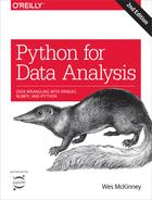
You can think of Period('2007',
'A-DEC') as being a sort of cursor pointing to a span of time,
subdivided by monthly periods. See Figure 11-1 for an illustration of this. For a
fiscal year ending on a month other than December,
the corresponding monthly subperiods are different:
In[164]:p=pd.Period('2007',freq='A-JUN')In[165]:pOut[165]:Period('2007','A-JUN')In[166]:p.asfreq('M','start')Out[166]:Period('2006-07','M')In[167]:p.asfreq('M','end')Out[167]:Period('2007-06','M')
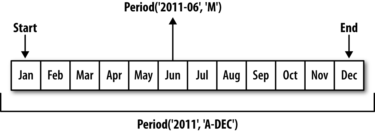
Figure 11-1. Period frequency conversion illustration
When you are converting from high to low frequency, pandas determines the superperiod depending on where the subperiod “belongs.” For example,
in A-JUN frequency, the month
Aug-2007 is actually part of the
2008 period:
In[168]:p=pd.Period('Aug-2007','M')In[169]:p.asfreq('A-JUN')Out[169]:Period('2008','A-JUN')
Whole PeriodIndex objects or
time series can be similarly converted with the same semantics:
In[170]:rng=pd.period_range('2006','2009',freq='A-DEC')In[171]:ts=pd.Series(np.random.randn(len(rng)),index=rng)In[172]:tsOut[172]:20061.60757820070.2003812008-0.8340682009-0.302988Freq:A-DEC,dtype:float64In[173]:ts.asfreq('M',how='start')Out[173]:2006-011.6075782007-010.2003812008-01-0.8340682009-01-0.302988Freq:M,dtype:float64
Here, the annual periods are replaced with monthly periods
corresponding to the first month falling within each annual period. If
we instead wanted the last business day of each year, we can use the
'B' frequency and indicate that we want the end of
the period:
In[174]:ts.asfreq('B',how='end')Out[174]:2006-12-291.6075782007-12-310.2003812008-12-31-0.8340682009-12-31-0.302988Freq:B,dtype:float64
Quarterly Period Frequencies
Quarterly data is standard in accounting, finance, and other fields. Much
quarterly data is reported relative to a fiscal year
end, typically the last calendar or business day of one of
the 12 months of the year. Thus, the period 2012Q4 has a different meaning depending on
fiscal year end. pandas supports all 12 possible quarterly frequencies
as Q-JAN through Q-DEC:
In[175]:p=pd.Period('2012Q4',freq='Q-JAN')In[176]:pOut[176]:Period('2012Q4','Q-JAN')
In the case of fiscal year ending in January, 2012Q4 runs from November through January,
which you can check by converting to daily frequency. See Figure 11-2 for an illustration.
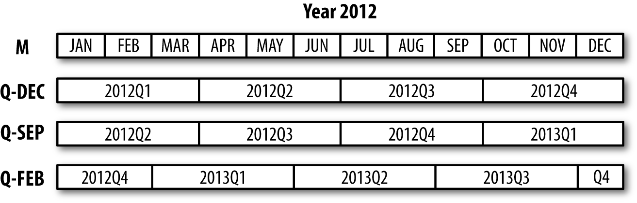
Figure 11-2. Different quarterly frequency conventions
In[177]:p.asfreq('D','start')Out[177]:Period('2011-11-01','D')In[178]:p.asfreq('D','end')Out[178]:Period('2012-01-31','D')
Thus, it’s possible to do easy period arithmetic; for example, to get the timestamp at 4 PM on the second-to-last business day of the quarter, you could do:
In[179]:p4pm=(p.asfreq('B','e')-1).asfreq('T','s')+16*60In[180]:p4pmOut[180]:Period('2012-01-30 16:00','T')In[181]:p4pm.to_timestamp()Out[181]:Timestamp('2012-01-30 16:00:00')
You can generate quarterly ranges using period_range.
Arithmetic is identical, too:
In[182]:rng=pd.period_range('2011Q3','2012Q4',freq='Q-JAN')In[183]:ts=pd.Series(np.arange(len(rng)),index=rng)In[184]:tsOut[184]:2011Q302011Q412012Q122012Q232012Q342012Q45Freq:Q-JAN,dtype:int64In[185]:new_rng=(rng.asfreq('B','e')-1).asfreq('T','s')+16*60In[186]:ts.index=new_rng.to_timestamp()In[187]:tsOut[187]:2010-10-2816:00:0002011-01-2816:00:0012011-04-2816:00:0022011-07-2816:00:0032011-10-2816:00:0042012-01-3016:00:005dtype:int64
Converting Timestamps to Periods (and Back)
Series and DataFrame objects indexed by timestamps can be converted to periods with
the to_period
method:
In[188]:rng=pd.date_range('2000-01-01',periods=3,freq='M')In[189]:ts=pd.Series(np.random.randn(3),index=rng)In[190]:tsOut[190]:2000-01-311.6632612000-02-29-0.9962062000-03-311.521760Freq:M,dtype:float64In[191]:pts=ts.to_period()In[192]:ptsOut[192]:2000-011.6632612000-02-0.9962062000-031.521760Freq:M,dtype:float64
Since periods refer to non-overlapping timespans, a timestamp can
only belong to a single period for a given frequency. While the
frequency of the new PeriodIndex is
inferred from the timestamps by default, you can specify any frequency
you want. There is also no problem with having duplicate periods in the
result:
In[193]:rng=pd.date_range('1/29/2000',periods=6,freq='D')In[194]:ts2=pd.Series(np.random.randn(6),index=rng)In[195]:ts2Out[195]:2000-01-290.2441752000-01-300.4233312000-01-31-0.6540402000-02-012.0891542000-02-02-0.0602202000-02-03-0.167933Freq:D,dtype:float64In[196]:ts2.to_period('M')Out[196]:2000-010.2441752000-010.4233312000-01-0.6540402000-022.0891542000-02-0.0602202000-02-0.167933Freq:M,dtype:float64
To convert back to timestamps, use to_timestamp:
In[197]:pts=ts2.to_period()In[198]:ptsOut[198]:2000-01-290.2441752000-01-300.4233312000-01-31-0.6540402000-02-012.0891542000-02-02-0.0602202000-02-03-0.167933Freq:D,dtype:float64In[199]:pts.to_timestamp(how='end')Out[199]:2000-01-290.2441752000-01-300.4233312000-01-31-0.6540402000-02-012.0891542000-02-02-0.0602202000-02-03-0.167933Freq:D,dtype:float64
Creating a PeriodIndex from Arrays
Fixed frequency datasets are sometimes stored with timespan information spread across multiple columns. For example, in this macroeconomic dataset, the year and quarter are in different columns:
In[200]:data=pd.read_csv('examples/macrodata.csv')In[201]:data.head(5)Out[201]:yearquarterrealgdprealconsrealinvrealgovtrealdpicpi\01959.01.02710.3491707.4286.898470.0451886.928.9811959.02.02778.8011733.7310.859481.3011919.729.1521959.03.02775.4881751.8289.226491.2601916.429.3531959.04.02785.2041753.7299.356484.0521931.329.3741960.01.02847.6991770.5331.722462.1991955.529.54m1tbilrateunemppopinflrealint0139.72.825.8177.1460.000.001141.73.085.1177.8302.340.742140.53.825.3178.6572.741.093140.04.335.6179.3860.274.064139.63.505.2180.0072.311.19In[202]:data.yearOut[202]:01959.011959.021959.031959.041960.051960.061960.071960.081961.091961.0...1932007.01942007.01952007.01962008.01972008.01982008.01992008.02002009.02012009.02022009.0Name:year,Length:203,dtype:float64In[203]:data.quarterOut[203]:01.012.023.034.041.052.063.074.081.092.0...1932.01943.01954.01961.01972.01983.01994.02001.02012.02023.0Name:quarter,Length:203,dtype:float64
By passing these arrays to PeriodIndex with a frequency, you can combine them to form an index for the DataFrame:
In[204]:index=pd.PeriodIndex(year=data.year,quarter=data.quarter,.....:freq='Q-DEC')In[205]:indexOut[205]:PeriodIndex(['1959Q1','1959Q2','1959Q3','1959Q4','1960Q1','1960Q2','1960Q3','1960Q4','1961Q1','1961Q2',...'2007Q2','2007Q3','2007Q4','2008Q1','2008Q2','2008Q3','2008Q4','2009Q1','2009Q2','2009Q3'],dtype='period[Q-DEC]',length=203,freq='Q-DEC')In[206]:data.index=indexIn[207]:data.inflOut[207]:1959Q10.001959Q22.341959Q32.741959Q40.271960Q12.311960Q20.141960Q32.701960Q41.211961Q1-0.401961Q21.47...2007Q22.752007Q33.452007Q46.382008Q12.822008Q28.532008Q3-3.162008Q4-8.792009Q10.942009Q23.372009Q33.56Freq:Q-DEC,Name:infl,Length:203,dtype:float64
11.6 Resampling and Frequency Conversion
Resampling refers to the process of converting a time series from one frequency to
another. Aggregating higher frequency data to lower frequency is
called downsampling, while converting
lower frequency to higher frequency is called upsampling. Not all resampling
falls into either of these categories; for example, converting W-WED (weekly on Wednesday) to W-FRI is neither upsampling nor
downsampling.
pandas objects are equipped with a resample method, which
is the workhorse function for all frequency conversion.
resample has a similar API to
groupby; you call resample to group
the data, then call an aggregation function:
In[208]:rng=pd.date_range('2000-01-01',periods=100,freq='D')In[209]:ts=pd.Series(np.random.randn(len(rng)),index=rng)In[210]:tsOut[210]:2000-01-010.6316342000-01-02-1.5943132000-01-03-1.5199372000-01-041.1087522000-01-051.2558532000-01-06-0.0243302000-01-07-2.0479392000-01-08-0.2726572000-01-09-1.6926152000-01-101.423830...2000-03-31-0.0078522000-04-01-1.6388062000-04-021.4012272000-04-031.7585392000-04-040.6289322000-04-05-0.4237762000-04-060.7897402000-04-070.9375682000-04-08-2.2532942000-04-09-1.772919Freq:D,Length:100,dtype:float64In[211]:ts.resample('M').mean()Out[211]:2000-01-31-0.1658932000-02-290.0786062000-03-310.2238112000-04-30-0.063643Freq:M,dtype:float64In[212]:ts.resample('M',kind='period').mean()Out[212]:2000-01-0.1658932000-020.0786062000-030.2238112000-04-0.063643Freq:M,dtype:float64
resample is a flexible and
high-performance method that can be used to process very large time
series. The examples in the following sections illustrate its semantics
and use. Table 11-5 summarizes some of its
options.
| Argument | Description |
|---|---|
freq | String or DateOffset indicating desired resampled frequency
(e.g., ‘M', ’5min', or Second(15)) |
axis | Axis to resample on; default axis=0 |
fill_method | How to interpolate when upsampling, as in 'ffill' or 'bfill'; by default does no
interpolation |
closed | In downsampling, which end of each interval is closed
(inclusive), 'right' or
'left' |
label | In downsampling, how to label the aggregated result, with
the 'right' or 'left' bin edge (e.g., the 9:30 to 9:35
five-minute interval could be labeled 9:30 or 9:35) |
loffset | Time adjustment to the bin labels, such as '-1s' / Second(-1) to shift the aggregate labels
one second earlier |
limit | When forward or backward filling, the maximum number of periods to fill |
kind | Aggregate to periods ('period') or timestamps ('timestamp'); defaults to the type of
index the time series has |
convention | When resampling periods, the convention ('start' or 'end') for converting the low-frequency
period to high frequency; defaults to 'end' |
Downsampling
Aggregating data to a regular, lower frequency is a pretty normal time series task. The
data you’re aggregating doesn’t need to be fixed frequently; the desired
frequency defines bin edges that are used to slice
the time series into pieces to aggregate. For example, to convert to
monthly, 'M' or 'BM', you need to chop up the data into one-month intervals. Each interval is said to be
half-open; a data point can only belong to one
interval, and the union of the intervals must make up the whole time
frame. There are a couple things to think about when using resample to downsample data:
Which side of each interval is closed
How to label each aggregated bin, either with the start of the interval or the end
To illustrate, let’s look at some one-minute data:
In[213]:rng=pd.date_range('2000-01-01',periods=12,freq='T')In[214]:ts=pd.Series(np.arange(12),index=rng)In[215]:tsOut[215]:2000-01-0100:00:0002000-01-0100:01:0012000-01-0100:02:0022000-01-0100:03:0032000-01-0100:04:0042000-01-0100:05:0052000-01-0100:06:0062000-01-0100:07:0072000-01-0100:08:0082000-01-0100:09:0092000-01-0100:10:00102000-01-0100:11:0011Freq:T,dtype:int64
Suppose you wanted to aggregate this data into five-minute chunks or bars by taking the sum of each group:
In[216]:ts.resample('5min',closed='right').sum()Out[216]:1999-12-3123:55:0002000-01-0100:00:00152000-01-0100:05:00402000-01-0100:10:0011Freq:5T,dtype:int64
The frequency you pass defines bin edges in five-minute
increments. By default, the
left bin edge is inclusive, so the
00:00 value is included in the
00:00 to 00:05 interval.1 Passing closed='right'
changes the interval to be closed on the right:
In[217]:ts.resample('5min',closed='right').sum()Out[217]:1999-12-3123:55:0002000-01-0100:00:00152000-01-0100:05:00402000-01-0100:10:0011Freq:5T,dtype:int64
The resulting time series is labeled by the timestamps from the
left side of each bin. By passing label='right' you can label them with the
right bin edge:
In[218]:ts.resample('5min',closed='right',label='right').sum()Out[218]:2000-01-0100:00:0002000-01-0100:05:00152000-01-0100:10:00402000-01-0100:15:0011Freq:5T,dtype:int64
See Figure 11-3 for an illustration of minute frequency data being resampled to five-minute frequency.
Figure 11-3. Five-minute resampling illustration of closed, label conventions
Lastly, you might want to shift the result index by some amount,
say subtracting one second from the right edge to make it more clear
which interval the timestamp refers to. To do this, pass a string or
date offset to loffset:
In[219]:ts.resample('5min',closed='right',.....:label='right',loffset='-1s').sum()Out[219]:1999-12-3123:59:5902000-01-0100:04:59152000-01-0100:09:59402000-01-0100:14:5911Freq:5T,dtype:int64
You also could have accomplished the effect of loffset by calling the shift method on the
result without the loffset.
Open-High-Low-Close (OHLC) resampling
In finance, a popular way to aggregate a time series is to compute
four values for each bucket: the first (open), last (close), maximum
(high), and minimal (low) values. By using the ohlc
aggregate function you will obtain a DataFrame having columns
containing these four aggregates, which are efficiently computed in a
single sweep of the data:
In[220]:ts.resample('5min').ohlc()Out[220]:openhighlowclose2000-01-0100:00:0004042000-01-0100:05:0059592000-01-0100:10:0010111011
Upsampling and Interpolation
When converting from a low frequency to a higher frequency, no aggregation is needed. Let’s consider a DataFrame with some weekly data:
In[221]:frame=pd.DataFrame(np.random.randn(2,4),.....:index=pd.date_range('1/1/2000',periods=2,.....:freq='W-WED'),.....:columns=['Colorado','Texas','New York','Ohio'])In[222]:frameOut[222]:ColoradoTexasNewYorkOhio2000-01-05-0.8964310.6772630.0365030.0871022000-01-12-0.0466620.9272380.482284-0.867130
When you are using an aggregation function with this data, there is only
one value per group, and missing values result in the gaps. We use the
asfreq method to convert to the higher frequency without any
aggregation:
In[223]:df_daily=frame.resample('D').asfreq()In[224]:df_dailyOut[224]:ColoradoTexasNewYorkOhio2000-01-05-0.8964310.6772630.0365030.0871022000-01-06NaNNaNNaNNaN2000-01-07NaNNaNNaNNaN2000-01-08NaNNaNNaNNaN2000-01-09NaNNaNNaNNaN2000-01-10NaNNaNNaNNaN2000-01-11NaNNaNNaNNaN2000-01-12-0.0466620.9272380.482284-0.867130
Suppose you wanted to fill forward each weekly value on the
non-Wednesdays. The same filling or interpolation methods available in the fillna
and reindex methods are available for
resampling:
In[225]:frame.resample('D').ffill()Out[225]:ColoradoTexasNewYorkOhio2000-01-05-0.8964310.6772630.0365030.0871022000-01-06-0.8964310.6772630.0365030.0871022000-01-07-0.8964310.6772630.0365030.0871022000-01-08-0.8964310.6772630.0365030.0871022000-01-09-0.8964310.6772630.0365030.0871022000-01-10-0.8964310.6772630.0365030.0871022000-01-11-0.8964310.6772630.0365030.0871022000-01-12-0.0466620.9272380.482284-0.867130
You can similarly choose to only fill a certain number of periods forward to limit how far to continue using an observed value:
In[226]:frame.resample('D').ffill(limit=2)Out[226]:ColoradoTexasNewYorkOhio2000-01-05-0.8964310.6772630.0365030.0871022000-01-06-0.8964310.6772630.0365030.0871022000-01-07-0.8964310.6772630.0365030.0871022000-01-08NaNNaNNaNNaN2000-01-09NaNNaNNaNNaN2000-01-10NaNNaNNaNNaN2000-01-11NaNNaNNaNNaN2000-01-12-0.0466620.9272380.482284-0.867130
Notably, the new date index need not overlap with the old one at all:
In[227]:frame.resample('W-THU').ffill()Out[227]:ColoradoTexasNewYorkOhio2000-01-06-0.8964310.6772630.0365030.0871022000-01-13-0.0466620.9272380.482284-0.867130
Resampling with Periods
Resampling data indexed by periods is similar to timestamps:
In[228]:frame=pd.DataFrame(np.random.randn(24,4),.....:index=pd.period_range('1-2000','12-2001',.....:freq='M'),.....:columns=['Colorado','Texas','New York','Ohio'])In[229]:frame[:5]Out[229]:ColoradoTexasNewYorkOhio2000-010.493841-0.1554341.3972861.5070552000-02-1.1794420.4431711.395676-0.5296582000-030.7873580.2488450.7432391.2677462000-041.302395-0.272154-0.051532-0.4677402000-05-1.0408160.4264190.312945-1.115689In[230]:annual_frame=frame.resample('A-DEC').mean()In[231]:annual_frameOut[231]:ColoradoTexasNewYorkOhio20000.5567030.0166310.111873-0.02744520010.0463030.1633440.251503-0.157276
Upsampling is more nuanced, as you must make a decision about which
end of the timespan in the new frequency to place the values before
resampling, just like the asfreq
method. The convention argument
defaults to 'start' but can also be
'end':
# Q-DEC: Quarterly, year ending in DecemberIn[232]:annual_frame.resample('Q-DEC').ffill()Out[232]:ColoradoTexasNewYorkOhio2000Q10.5567030.0166310.111873-0.0274452000Q20.5567030.0166310.111873-0.0274452000Q30.5567030.0166310.111873-0.0274452000Q40.5567030.0166310.111873-0.0274452001Q10.0463030.1633440.251503-0.1572762001Q20.0463030.1633440.251503-0.1572762001Q30.0463030.1633440.251503-0.1572762001Q40.0463030.1633440.251503-0.157276In[233]:annual_frame.resample('Q-DEC',convention='end').ffill()Out[233]:ColoradoTexasNewYorkOhio2000Q40.5567030.0166310.111873-0.0274452001Q10.5567030.0166310.111873-0.0274452001Q20.5567030.0166310.111873-0.0274452001Q30.5567030.0166310.111873-0.0274452001Q40.0463030.1633440.251503-0.157276
Since periods refer to timespans, the rules about upsampling and downsampling are more rigid:
In downsampling, the target frequency must be a subperiod of the source frequency.
In upsampling, the target frequency must be a superperiod of the source frequency.
If these rules are not satisfied, an exception will be raised.
This mainly affects the quarterly, annual, and weekly frequencies; for
example, the timespans defined by Q-MAR only line up with A-MAR, A-JUN, A-SEP, and A-DEC:
In[234]:annual_frame.resample('Q-MAR').ffill()Out[234]:ColoradoTexasNewYorkOhio2000Q40.5567030.0166310.111873-0.0274452001Q10.5567030.0166310.111873-0.0274452001Q20.5567030.0166310.111873-0.0274452001Q30.5567030.0166310.111873-0.0274452001Q40.0463030.1633440.251503-0.1572762002Q10.0463030.1633440.251503-0.1572762002Q20.0463030.1633440.251503-0.1572762002Q30.0463030.1633440.251503-0.157276
11.7 Moving Window Functions
An important class of array transformations used for time series operations are statistics and other functions evaluated over a sliding window or with exponentially decaying weights. This can be useful for smoothing noisy or gappy data. I call these moving window functions, even though it includes functions without a fixed-length window like exponentially weighted moving average. Like other statistical functions, these also automatically exclude missing data.
Before digging in, we can load up some time series data and resample it to business day frequency:
In[235]:close_px_all=pd.read_csv('examples/stock_px_2.csv',.....:parse_dates=True,index_col=0)In[236]:close_px=close_px_all[['AAPL','MSFT','XOM']]In[237]:close_px=close_px.resample('B').ffill()
I now introduce the rolling operator, which behaves similarly to resample and
groupby. It can be called on a Series or DataFrame
along with a window (expressed as a
number of periods; see Figure 11-4 for the plot
created):
In[238]:close_px.AAPL.plot()Out[238]:<matplotlib.axes._subplots.AxesSubplotat0x7fa59eaf0b00>In[239]:close_px.AAPL.rolling(250).mean().plot()
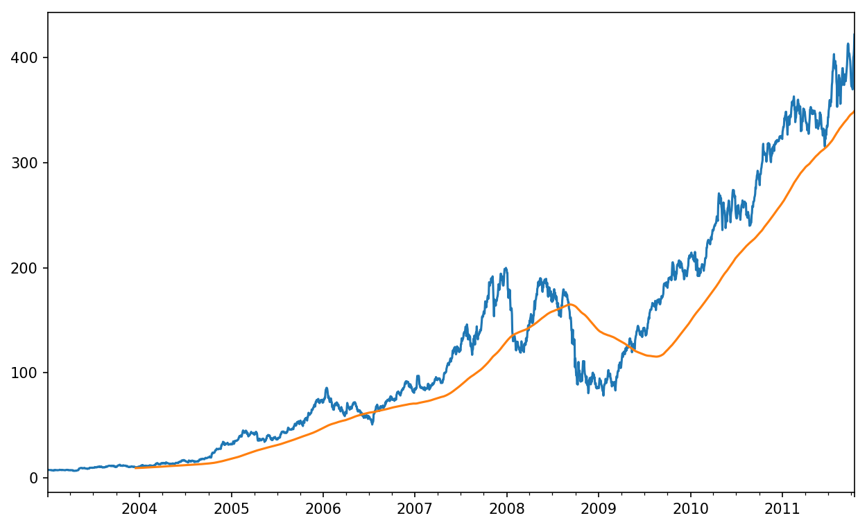
Figure 11-4. Apple Price with 250-day MA
The expression rolling(250) is similar in
behavior to groupby, but instead of grouping it creates
an object that enables grouping over a 250-day sliding window. So here we
have the 250-day moving window average of Apple’s stock price.
By default rolling functions require all of the values in the window
to be non-NA. This behavior can be changed to account for missing data
and, in particular, the fact that you will have fewer than window periods of data at the beginning of the
time series (see Figure 11-5):
In[241]:appl_std250=close_px.AAPL.rolling(250,min_periods=10).std()In[242]:appl_std250[5:12]Out[242]:2003-01-09NaN2003-01-10NaN2003-01-13NaN2003-01-14NaN2003-01-150.0774962003-01-160.0747602003-01-170.112368Freq:B,Name:AAPL,dtype:float64In[243]:appl_std250.plot()
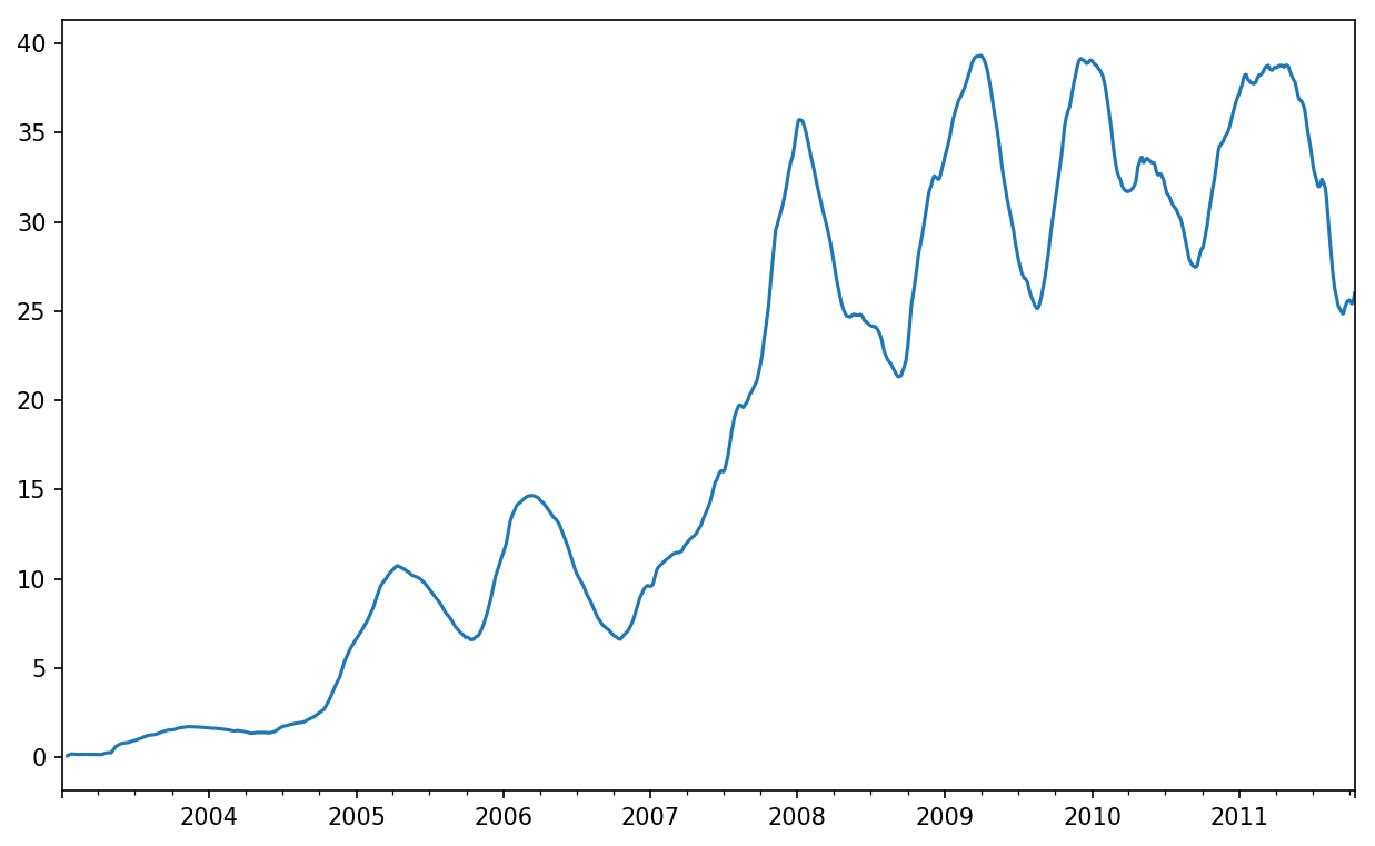
Figure 11-5. Apple 250-day daily return standard deviation
In order to compute an expanding window mean,
use the expanding operator instead of
rolling. The expanding mean starts the time window from
the beginning of the time series and increases the size of the window
until it encompasses the whole series. An expanding window mean on the
apple_std250 time series looks like this:
In[244]:expanding_mean=appl_std250.expanding().mean()
Calling a moving window function on a DataFrame applies the transformation to each column (see Figure 11-6):
In[246]:close_px.rolling(60).mean().plot(logy=True)
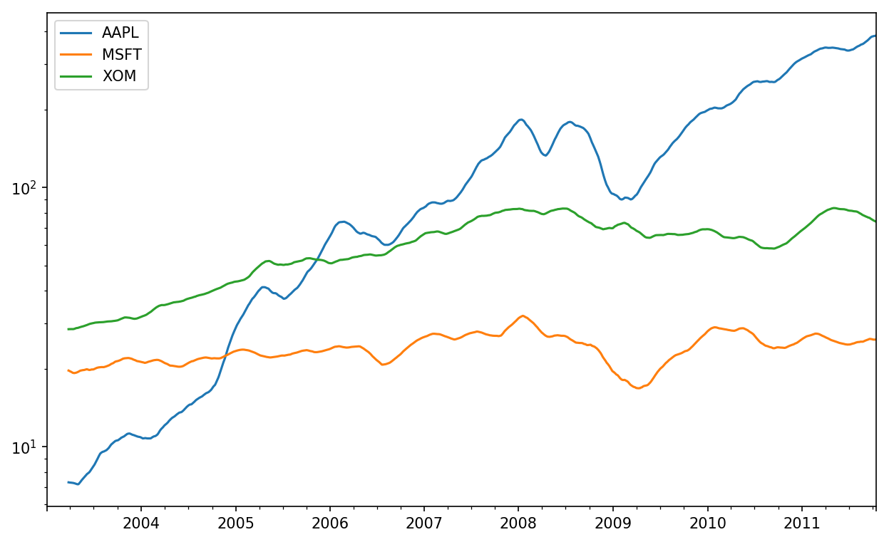
Figure 11-6. Stocks prices 60-day MA (log Y-axis)
The rolling function also accepts a string indicating a fixed-size time offset
rather than a set number of periods. Using this notation can be useful for
irregular time series. These are the same strings that you can pass to
resample. For example, we could compute a 20-day
rolling mean like so:
In[247]:close_px.rolling('20D').mean()Out[247]:AAPLMSFTXOM2003-01-027.40000021.11000029.2200002003-01-037.42500021.12500029.2300002003-01-067.43333321.25666729.4733332003-01-077.43250021.42500029.3425002003-01-087.40200021.40200029.2400002003-01-097.39166721.49000029.2733332003-01-107.38714321.55857129.2385712003-01-137.37875021.63375029.1975002003-01-147.37000021.71777829.1944442003-01-157.35500021.75700029.152000............2011-10-03398.00214325.89071472.4135712011-10-04396.80214325.80785772.4271432011-10-05395.75142925.72928672.4228572011-10-06394.09928625.67357172.3757142011-10-07392.47933325.71200072.4546672011-10-10389.35142925.60214372.5278572011-10-11388.50500025.67428672.8350002011-10-12388.53142925.81000073.4007142011-10-13388.82642925.96142973.9050002011-10-14391.03800026.04866774.185333[2292rowsx3columns]
Exponentially Weighted Functions
An alternative to using a static window size with equally weighted observations is to specify a constant decay factor to give more weight to more recent observations. There are a couple of ways to specify the decay factor. A popular one is using a span, which makes the result comparable to a simple moving window function with window size equal to the span.
Since an exponentially weighted statistic places more weight on more recent observations, it “adapts” faster to changes compared with the equal-weighted version.
pandas has the ewm operator to go along with rolling and
expanding. Here’s an example comparing a 60-day
moving average of Apple’s stock price with an EW moving average with
span=60 (see Figure 11-7):
In[249]:aapl_px=close_px.AAPL['2006':'2007']In[250]:ma60=aapl_px.rolling(30,min_periods=20).mean()In[251]:ewma60=aapl_px.ewm(span=30).mean()In[252]:ma60.plot(style='k--',label='Simple MA')Out[252]:<matplotlib.axes._subplots.AxesSubplotat0x7fa59e5df908>In[253]:ewma60.plot(style='k-',label='EW MA')Out[253]:<matplotlib.axes._subplots.AxesSubplotat0x7fa59e5df908>In[254]:plt.legend()
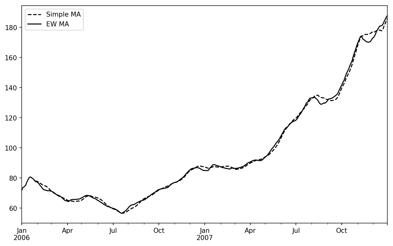
Figure 11-7. Simple moving average versus exponentially weighted
Binary Moving Window Functions
Some statistical operators, like correlation and covariance, need to operate on two time series. As an example, financial analysts are often interested in a stock’s correlation to a benchmark index like the S&P 500. To have a look at this, we first compute the percent change for all of our time series of interest:
In[256]:spx_px=close_px_all['SPX']In[257]:spx_rets=spx_px.pct_change()In[258]:returns=close_px.pct_change()
The corr aggregation function after we call rolling can then compute
the rolling correlation with spx_rets (see Figure 11-8 for the resulting plot):
In[259]:corr=returns.AAPL.rolling(125,min_periods=100).corr(spx_rets)In[260]:corr.plot()
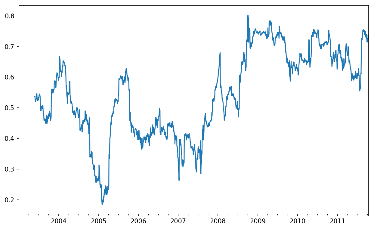
Figure 11-8. Six-month AAPL return correlation to S&P 500
Suppose you wanted to compute the correlation of the S&P 500
index with many stocks at once. Writing a loop and creating a new
DataFrame would be easy but might get repetitive, so if you pass a
Series and a DataFrame, a function like rolling_corr will
compute the correlation of the Series (spx_rets, in this case) with each column in
the DataFrame (see Figure 11-9 for the plot of
the result):
In[262]:corr=returns.rolling(125,min_periods=100).corr(spx_rets)In[263]:corr.plot()
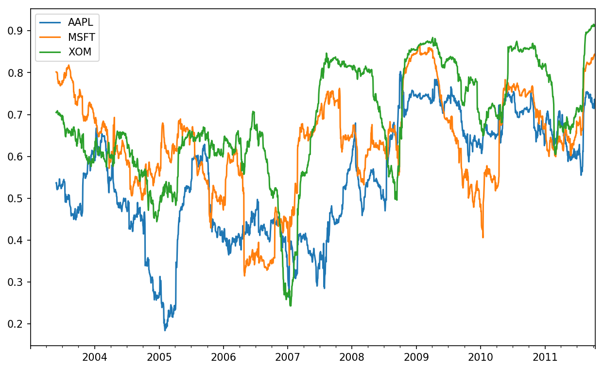
Figure 11-9. Six-month return correlations to S&P 500
User-Defined Moving Window Functions
The apply method on
rolling and related methods provides a means to apply an array
function of your own devising over a moving window. The only requirement
is that the function produce a single value (a reduction) from each
piece of the array. For example, while we can compute sample quantiles
using rolling(...).quantile(q), we
might be interested in the percentile rank of a particular value over
the sample. The scipy.stats.percentileofscore function
does just this (see Figure 11-10 for
the resulting plot):
In[265]:fromscipy.statsimportpercentileofscoreIn[266]:score_at_2percent=lambdax:percentileofscore(x,0.02)In[267]:result=returns.AAPL.rolling(250).apply(score_at_2percent)In[268]:result.plot()
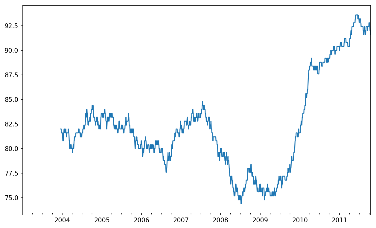
Figure 11-10. Percentile rank of 2% AAPL return over one-year window
If you don’t have SciPy installed already, you can install it with conda or pip.
11.8 Conclusion
Time series data calls for different types of analysis and data transformation tools than the other types of data we have explored in previous chapters.
In the following chapters, we will move on to some advanced pandas methods and show how to start using modeling libraries like statsmodels and scikit-learn.
1 The choice of the default values for closed and label might seem a bit odd to some users.
In practice the choice is somewhat arbitrary; for some target
frequencies, closed='left' is
preferable, while for others closed='right' makes more sense. The
important thing is that you keep in mind exactly how you are
segmenting the data.