Table of Contents for
Python for Data Analysis, 2nd Edition
 Python for Data Analysis, 2nd Edition
Published by
O'Reilly Media, Inc., 2017
Python for Data Analysis, 2nd Edition
Published by
O'Reilly Media, Inc., 2017
- nav
- Cover
- Python for Data Analysis
- Python for Data Analysis
- Preface
- Preliminaries
- Python Language Basics, IPython, and Jupyter Notebooks
- Built-in Data Structures, Functions, and Files
- NumPy Basics: Arrays and Vectorized Computation
- Getting Started with pandas
- Data Loading, Storage, and File Formats
- Data Cleaning and Preparation
- Data Wrangling: Join, Combine, and Reshape
- Plotting and Visualization
- Data Aggregation and Group Operations
- Time Series
- Advanced pandas
- Introduction to Modeling Libraries in Python
- Data Analysis Examples
- Advanced NumPy
- More on the IPython System
- Index
- About the Author
- Colophon
Chapter 2. Python Language Basics, IPython, and Jupyter Notebooks
When I wrote the first edition of this book in 2011 and 2012, there were fewer resources available for learning about doing data analysis in Python. This was partially a chicken-and-egg problem; many libraries that we now take for granted, like pandas, scikit-learn, and statsmodels, were comparatively immature back then. In 2017, there is now a growing literature on data science, data analysis, and machine learning, supplementing the prior works on general-purpose scientific computing geared toward computational scientists, physicists, and professionals in other research fields. There are also excellent books about learning the Python programming language itself and becoming an effective software engineer.
As this book is intended as an introductory text in working with data in Python, I feel it is valuable to have a self-contained overview of some of the most important features of Python’s built-in data structures and libraries from the perspective of data manipulation. So, I will only present roughly enough information in this chapter and Chapter 3 to enable you to follow along with the rest of the book.
In my opinion, it is not necessary to become proficient at building good software in Python to be able to productively do data analysis. I encourage you to use the IPython shell and Jupyter notebooks to experiment with the code examples and to explore the documentation for the various types, functions, and methods. While I’ve made best efforts to present the book material in an incremental form, you may occasionally encounter things that have not yet been fully introduced.
Much of this book focuses on table-based analytics and data preparation tools for working with large datasets. In order to use those tools you must often first do some munging to corral messy data into a more nicely tabular (or structured) form. Fortunately, Python is an ideal language for rapidly whipping your data into shape. The greater your facility with Python the language, the easier it will be for you to prepare new datasets for analysis.
Some of the tools in this book are best explored from a live IPython or Jupyter session. Once you learn how to start up IPython and Jupyter, I recommend that you follow along with the examples so you can experiment and try different things. As with any keyboard-driven console-like environment, developing muscle-memory for the common commands is also part of the learning curve.
Note
There are introductory Python concepts that this chapter does not cover, like classes and object-oriented programming, which you may find useful in your foray into data analysis in Python.
To deepen your Python language knowledge, I recommend that you supplement this chapter with the official Python tutorial and potentially one of the many excellent books on general-purpose Python programming. Some recommendations to get you started include:
Python Cookbook, Third Edition, by David Beazley and Brian K. Jones (O’Reilly)
Fluent Python by Luciano Ramalho (O’Reilly)
Effective Python by Brett Slatkin (Pearson)
2.1 The Python Interpreter
Python is an interpreted language. The Python
interpreter runs a program by executing one statement at a time. The
standard interactive Python interpreter can be invoked on the command line
with the python
command:
$ python
Python 3.6.0 | packaged by conda-forge | (default, Jan 13 2017, 23:17:12)
[GCC 4.8.2 20140120 (Red Hat 4.8.2-15)] on linux
Type "help", "copyright", "credits" or "license" for more information.
>>> a = 5
>>> print(a)
5
The >>> you see is the prompt where you’ll type
code expressions. To exit the Python interpreter and return to the command
prompt, you can either type exit() or press Ctrl-D.
Running Python programs is as simple as calling python with a .py file
as its first argument. Suppose we had created
hello_world.py with these contents:
('Hello world')
You can run it by executing the following command (the hello_world.py file must be in your current working terminal directory):
$ python hello_world.py
Hello world
While some Python programmers execute all of their Python code in
this way, those doing data analysis or scientific computing make use of
IPython, an enhanced Python interpreter, or Jupyter notebooks, web-based
code notebooks originally created within the IPython project. I give an
introduction to using IPython and Jupyter in this chapter and have
included a deeper look at IPython functionality in Appendix A. When you use the %run command,
IPython executes the code in the specified file in the same process,
enabling you to explore the results interactively when it’s done:
$ipythonPython3.6.0|packagedbyconda-forge|(default,Jan132017,23:17:12)Type"copyright","credits"or"license"formoreinformation.IPython5.1.0--AnenhancedInteractivePython.?->IntroductionandoverviewofIPython's features.%quickref->Quickreference.help->Python's own help system.object?->Detailsabout'object',use'object??'forextradetails.In[1]:%runhello_world.pyHelloworldIn[2]:
The default IPython prompt adopts the numbered In [2]: style compared with the standard
>>> prompt.
2.2 IPython Basics
In this section, we’ll get you up and running with the IPython shell and Jupyter notebook, and introduce you to some of the essential concepts.
Running the IPython Shell
You can launch the IPython shell on the command line just like launching the
regular Python interpreter except with the ipython command:
$ ipython
Python 3.6.0 | packaged by conda-forge | (default, Jan 13 2017, 23:17:12)
Type "copyright", "credits" or "license" for more information.

IPython 5.1.0 -- An enhanced Interactive Python.
?         -> Introduction and overview of IPython's features.
%quickref -> Quick reference.
help      -> Python's own help system.
object?   -> Details about 'object', use 'object??' for extra details.

In [1]: a = 5

In [2]: a
Out[2]: 5
You can execute arbitrary Python statements by typing them in and pressing Return (or Enter). When you type just a variable into IPython, it renders a string representation of the object:
In[5]:importnumpyasnpIn[6]:data={i:np.random.randn()foriinrange(7)}In[7]:dataOut[7]:{0:-0.20470765948471295,1:0.47894333805754824,2:-0.5194387150567381,3:-0.55573030434749,4:1.9657805725027142,5:1.3934058329729904,6:0.09290787674371767}
The first two lines are Python code statements; the second
statement creates a variable named data that refers
to a newly created Python dictionary. The last line prints the value of
data in the console.
Many kinds of Python objects are formatted to be more readable, or
pretty-printed, which is distinct from normal
printing with print. If you printed
the above data variable in the standard Python
interpreter, it would be much less readable:
>>>fromnumpy.randomimportrandn>>>data={i:randn()foriinrange(7)}>>>(data){0:-1.5948255432744511,1:0.10569006472787983,2:1.972367135977295,3:0.15455217573074576,4:-0.24058577449429575,5:-1.2904897053651216,6:0.3308507317325902}
IPython also provides facilities to execute arbitrary blocks of code (via a somewhat glorified copy-and-paste approach) and whole Python scripts. You can also use the Jupyter notebook to work with larger blocks of code, as we’ll soon see.
Running the Jupyter Notebook
One of the major components of the Jupyter project is the notebook, a type of interactive document for code, text (with or without markup), data visualizations, and other output. The Jupyter notebook interacts with kernels, which are implementations of the Jupyter interactive computing protocol in any number of programming languages. Python’s Jupyter kernel uses the IPython system for its underlying behavior.
To start up Jupyter, run the command jupyter notebook in a
terminal:
$ jupyter notebook
[I 15:20:52.739 NotebookApp] Serving notebooks from local directory:
/home/wesm/code/pydata-book
[I 15:20:52.739 NotebookApp] 0 active kernels
[I 15:20:52.739 NotebookApp] The Jupyter Notebook is running at:
http://localhost:8888/
[I 15:20:52.740 NotebookApp] Use Control-C to stop this server and shut down
all kernels (twice to skip confirmation).
Created new window in existing browser session.
On many platforms, Jupyter will automatically open up in your
default web browser (unless you start it with
--no-browser). Otherwise, you can navigate to the
HTTP address printed when you started the notebook, here
http://localhost:8888/. See Figure 2-1 for what this looks like in Google
Chrome.
Note
Many people use Jupyter as a local computing environment, but it can also be deployed on servers and accessed remotely. I won’t cover those details here, but encourage you to explore this topic on the internet if it’s relevant to your needs.
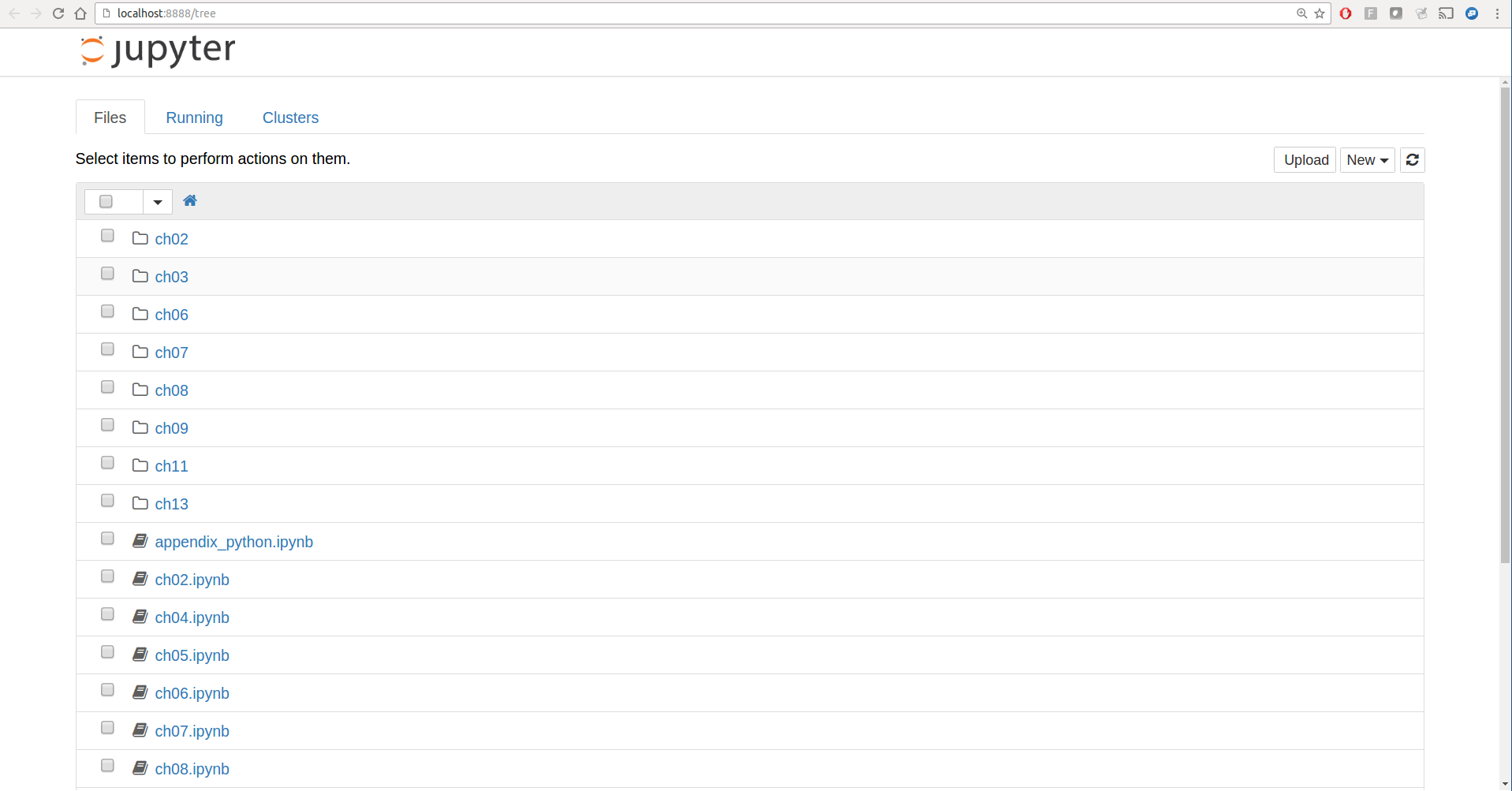
Figure 2-1. Jupyter notebook landing page
To create a new notebook, click the New button and select the “Python 3” or “conda [default]” option. You should see something like Figure 2-2. If this is your first time, try clicking on the empty code “cell” and entering a line of Python code. Then press Shift-Enter to execute it.
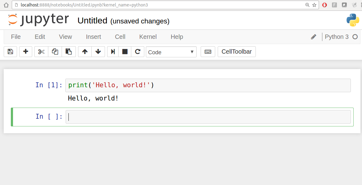
Figure 2-2. Jupyter new notebook view
When you save the notebook (see “Save and Checkpoint” under the notebook File menu), it creates a file with the extension .ipynb. This is a self-contained file format that contains all of the content (including any evaluated code output) currently in the notebook. These can be loaded and edited by other Jupyter users. To load an existing notebook, put the file in the same directory where you started the notebook process (or in a subfolder within it), then double-click the name from the landing page. You can try it out with the notebooks from my wesm/pydata-book repository on GitHub. See Figure 2-3.
While the Jupyter notebook can feel like a distinct experience from the IPython shell, nearly all of the commands and tools in this chapter can be used in either environment.
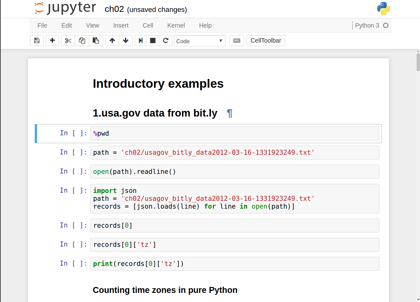
Figure 2-3. Jupyter example view for an existing notebook
Tab Completion
On the surface, the IPython shell looks like a cosmetically different version
of the standard terminal Python interpreter (invoked with
python). One of the major improvements over the
standard Python shell is tab completion, found in
many IDEs or other interactive computing analysis environments. While
entering expressions in the shell, pressing the Tab key will search the
namespace for any variables (objects, functions, etc.) matching the
characters you have typed so far:
In [1]: an_apple = 27

In [2]: an_example = 42

In [3]: an<Tab>
an_apple    and         an_example  any
In this example, note that IPython displayed both the two
variables I defined as well as the Python keyword and and built-in function any.
Naturally, you can also complete methods and attributes on any object
after typing a period:
In [3]: b = [1, 2, 3]

In [4]: b.<Tab>
b.append  b.count   b.insert  b.reverse
b.clear   b.extend  b.pop     b.sort
b.copy    b.index   b.remove
The same goes for modules:
In [1]: import datetime

In [2]: datetime.<Tab>
datetime.date          datetime.MAXYEAR       datetime.timedelta
datetime.datetime      datetime.MINYEAR       datetime.timezone
datetime.datetime_CAPI datetime.time          datetime.tzinfo
In the Jupyter notebook and newer versions of IPython (5.0 and higher), the autocompletions show up in a drop-down box rather than as text output.
Note
Note that IPython by default hides methods and attributes starting with underscores, such as magic methods and internal “private” methods and attributes, in order to avoid cluttering the display (and confusing novice users!). These, too, can be tab-completed, but you must first type an underscore to see them. If you prefer to always see such methods in tab completion, you can change this setting in the IPython configuration. See the IPython documentation to find out how to do this.
Tab completion works in many contexts outside of searching the interactive namespace and completing object or module attributes. When typing anything that looks like a file path (even in a Python string), pressing the Tab key will complete anything on your computer’s filesystem matching what you’ve typed:
In [7]: datasets/movielens/<Tab>datasets/movielens/movies.dat datasets/movielens/README datasets/movielens/ratings.dat datasets/movielens/users.dat In [7]: path = 'datasets/movielens/<Tab>datasets/movielens/movies.dat datasets/movielens/README datasets/movielens/ratings.dat datasets/movielens/users.dat
Combined with the %run command
(see “The %run Command”), this functionality
can save you many keystrokes.
Another area where tab completion saves time is in the completion
of function keyword arguments (and including the = sign!). See Figure 2-4.
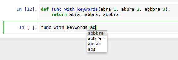
Figure 2-4. Autocomplete function keywords in Jupyter notebook
Introspection
Using a question mark (?)
before or after a variable will display some general information about
the object:
In[8]:b=[1,2,3]In[9]:b?Type:listStringForm:[1,2,3]Length:3Docstring:list()->newemptylistlist(iterable)->newlistinitializedfromiterable's itemsIn[10]:?Docstring:(value,...,sep=' ',end='\n',file=sys.stdout,flush=False)Printsthevaluestoastream,ortosys.stdoutbydefault.Optionalkeywordarguments:file:afile-likeobject(stream);defaultstothecurrentsys.stdout.sep:stringinsertedbetweenvalues,defaultaspace.end:stringappendedafterthelastvalue,defaultanewline.flush:whethertoforciblyflushthestream.Type:builtin_function_or_method
This is referred to as object introspection. If the object is a function or instance method, the docstring, if defined, will also be shown. Suppose we’d written the following function (which you can reproduce in IPython or Jupyter):
defadd_numbers(a,b):"""Add two numbers togetherReturns-------the_sum : type of arguments"""returna+b
Then using ? shows us the
docstring:
In[11]:add_numbers?Signature:add_numbers(a,b)Docstring:AddtwonumberstogetherReturns-------the_sum:typeofargumentsFile:<ipython-input-9-6a548a216e27>Type:function
Using ?? will also show the
function’s source code if possible:
In[12]:add_numbers??Signature:add_numbers(a,b)Source:defadd_numbers(a,b):"""Add two numbers togetherReturns-------the_sum : type of arguments"""returna+bFile:<ipython-input-9-6a548a216e27>Type:function
? has a final usage, which is
for searching the IPython namespace in a manner similar to the standard
Unix or Windows command line. A number of characters combined with the wildcard (*) will show all names matching the wildcard expression. For
example, we could get a list of all functions in the top-level NumPy
namespace containing load:
In[13]:np.*load*?np.__loader__np.loadnp.loadsnp.loadtxtnp.pkgload
The %run Command
You can run any file as a Python program inside the environment of your
IPython session using the %run
command. Suppose you had the following simple script stored in
ipython_script_test.py:
deff(x,y,z):return(x+y)/za=5b=6c=7.5result=f(a,b,c)
You can execute this by passing the filename to %run:
In[14]:%runipython_script_test.py
The script is run in an empty namespace (with no imports
or other variables defined) so that the behavior should be identical to
running the program on the command line using python script.py. All of the variables
(imports, functions, and globals) defined in the file (up until an
exception, if any, is raised) will then be accessible in the IPython
shell:
In[15]:cOut[15]:7.5In[16]:resultOut[16]:1.4666666666666666
If a Python script expects command-line arguments (to be found in
sys.argv), these can be passed after
the file path as though run on the command line.
Note
Should you wish to give a script access to variables already
defined in the interactive IPython namespace, use %run -i instead of plain %run.
In the Jupyter notebook, you may also use the related %load magic function, which
imports a script into a code cell:
>>>%loadipython_script_test.pydeff(x,y,z):return(x+y)/za=5b=6c=7.5result=f(a,b,c)
Interrupting running code
Pressing Ctrl-C while any code is running, whether a script through %run or a long-running command, will cause a
KeyboardInterrupt to be raised. This will cause nearly all Python programs to
stop immediately except in certain unusual cases.
Warning
When a piece of Python code has called into some compiled extension modules, pressing Ctrl-C will not always cause the program execution to stop immediately. In such cases, you will have to either wait until control is returned to the Python interpreter, or in more dire circumstances, forcibly terminate the Python process.
Executing Code from the Clipboard
If you are using the Jupyter notebook, you can copy and paste code into any code cell and execute it. It is also possible to run code from the clipboard in the IPython shell. Suppose you had the following code in some other application:
x=5y=7ifx>5:x+=1y=8
The most foolproof methods are the %paste and
%cpaste magic functions. %paste takes whatever text is in the clipboard
and executes it as a single block in the shell:
In[17]:%pastex=5y=7ifx>5:x+=1y=8## -- End pasted text --
%cpaste is similar, except that
it gives you a special prompt for pasting code into:
In[18]:%cpastePastingcode;enter'--'aloneonthelinetostoporuseCtrl-D.:x=5:y=7:ifx>5::x+=1::y=8:--
With the %cpaste block, you
have the freedom to paste as much code as you like before executing it.
You might decide to use %cpaste in
order to look at the pasted code before executing it. If you
accidentally paste the wrong code, you can break out of the %cpaste prompt by pressing Ctrl-C.
Terminal Keyboard Shortcuts
IPython has many keyboard shortcuts for navigating the prompt (which will be familiar to users of the Emacs text editor or the Unix bash shell) and interacting with the shell’s command history. Table 2-1 summarizes some of the most commonly used shortcuts. See Figure 2-5 for an illustration of a few of these, such as cursor movement.
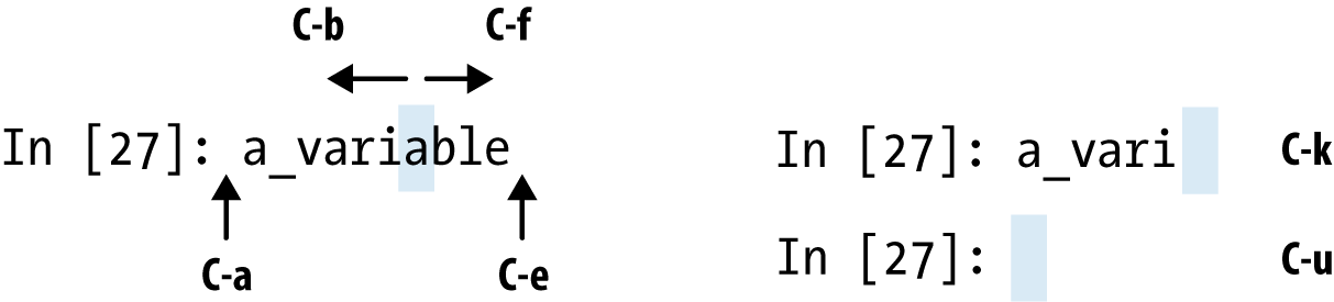
Figure 2-5. Illustration of some keyboard shortcuts in the IPython shell
Note that Jupyter notebooks have a largely separate set of keyboard shortcuts for navigation and editing. Since these shortcuts have evolved more rapidly than IPython’s, I encourage you to explore the integrated help system in the Jupyter notebook’s menus.
About Magic Commands
IPython’s special commands (which are not built into Python itself) are known as
“magic” commands. These are designed to facilitate common tasks and
enable you to easily control the behavior of the IPython system. A magic
command is any command prefixed by the percent symbol %. For
example, you can check the execution time of any Python statement, such
as a matrix multiplication, using the %timeit magic function (which will be
discussed in more detail later):
In[20]:a=np.random.randn(100,100)In[20]:%timeitnp.dot(a,a)10000loops,bestof3:20.9µsperloop
Magic commands can be viewed as command-line programs to be run
within the IPython system. Many of them have additional “command-line”
options, which can all be viewed (as you might expect) using ?:
In[21]:%debug?Docstring:::%debug[--breakpointFILE:LINE][statement[statement...]]Activatetheinteractivedebugger.Thismagiccommandsupporttwowaysofactivatingdebugger.Oneistoactivatedebuggerbeforeexecutingcode.Thisway,youcansetabreakpoint,tostepthroughthecodefromthepoint.Youcanusethismodebygivingstatementstoexecuteandoptionallyabreakpoint.Theotheroneistoactivatedebuggerinpost-mortemmode.Youcanactivatethismodesimplyrunning%debugwithoutanyargument.Ifanexceptionhasjustoccurred,thisletsyouinspectitsstackframesinteractively.Notethatthiswillalwaysworkonlyonthelasttracebackthatoccurred,soyoumustcallthisquicklyafteranexceptionthatyouwishtoinspecthasfired,becauseifanotheroneoccurs,itclobbersthepreviousone.IfyouwantIPythontoautomaticallydothisoneveryexception,seethe%pdbmagicformoredetails.positionalarguments:statementCodetorunindebugger.Youcanomitthisincellmagicmode.optionalarguments:--breakpoint<FILE:LINE>,-b<FILE:LINE>SetbreakpointatLINEinFILE.
Magic functions can be used by default without the percent sign,
as long as no variable is defined with the same name as the magic
function in question. This feature is called automagic and can be
enabled or disabled with %automagic.
Some magic functions behave like Python functions and their output can be assigned to a variable:
In[22]:%pwdOut[22]:'/home/wesm/code/pydata-bookIn[23]:foo=%pwdIn[24]:fooOut[24]:'/home/wesm/code/pydata-book'
Since IPython’s documentation is accessible from within the
system, I encourage you to explore all of the special commands available
by typing %quickref or %magic. Table 2-2
highlights some of the most critical ones for being productive in
interactive computing and Python development in IPython.
Matplotlib Integration
One reason for IPython’s popularity in analytical computing is that it
integrates well with data visualization and other user interface
libraries like matplotlib. Don’t worry if you have never used matplotlib
before; it will be discussed in more detail later in this book.
The %matplotlib magic function
configures its integration with the IPython shell or Jupyter notebook.
This is important, as otherwise plots you create will either not appear
(notebook) or take control of the session until closed (shell).
In the IPython shell, running %matplotlib sets
up the integration so you can create multiple plot windows without
interfering with the console session:
In[26]:%matplotlibUsingmatplotlibbackend:Qt4Agg
In Jupyter, the command is a little different (Figure 2-6):
In[26]:%matplotlibinline
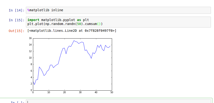
Figure 2-6. Jupyter inline matplotlib plotting
2.3 Python Language Basics
In this section, I will give you an overview of essential Python programming concepts and language mechanics. In the next chapter, I will go into more detail about Python’s data structures, functions, and other built-in tools.
Language Semantics
The Python language design is distinguished by its emphasis on readability, simplicity, and explicitness. Some people go so far as to liken it to “executable pseudocode.”
Indentation, not braces
Python uses whitespace (tabs or spaces) to structure code instead of
using braces as in many other languages like R, C++, Java, and Perl.
Consider a for loop from a sorting
algorithm:
forxinarray:ifx<pivot:less.append(x)else:greater.append(x)
A colon denotes the start of an indented code block after which all of the code must be indented by the same amount until the end of the block.
Love it or hate it, significant whitespace is a fact of life for Python programmers, and in my experience it can make Python code more readable than other languages I’ve used. While it may seem foreign at first, you will hopefully grow accustomed in time.
Note
I strongly recommend using four spaces as your default indentation and replacing tabs with four spaces. Many text editors have a setting that will replace tab stops with spaces automatically (do this!). Some people use tabs or a different number of spaces, with two spaces not being terribly uncommon. By and large, four spaces is the standard adopted by the vast majority of Python programmers, so I recommend doing that in the absence of a compelling reason otherwise.
As you can see by now, Python statements also do not need to be terminated by semicolons. Semicolons can be used, however, to separate multiple statements on a single line:
a = 5; b = 6; c = 7
Putting multiple statements on one line is generally discouraged in Python as it often makes code less readable.
Everything is an object
An important characteristic of the Python language is the consistency of its object model. Every number, string, data structure, function, class, module, and so on exists in the Python interpreter in its own “box,” which is referred to as a Python object. Each object has an associated type (e.g., string or function) and internal data. In practice this makes the language very flexible, as even functions can be treated like any other object.
Comments
Any text preceded by the hash mark (pound sign) #
is ignored by the Python interpreter. This is often used to add
comments to code. At times you may also want to exclude certain blocks
of code without deleting them. An easy solution is to
comment out the code:
results=[]forlineinfile_handle:# keep the empty lines for now# if len(line) == 0:# continueresults.append(line.replace('foo','bar'))
Comments can also occur after a line of executed code. While some programmers prefer comments to be placed in the line preceding a particular line of code, this can be useful at times:
("Reached this line")# Simple status report
Function and object method calls
You call functions using parentheses and passing zero or more arguments, optionally assigning the returned value to a variable:
result=f(x,y,z)g()
Almost every object in Python has attached functions, known as methods, that have access to the object’s internal contents. You can call them using the following syntax:
obj.some_method(x,y,z)
Functions can take both positional and keyword arguments:
result=f(a,b,c,d=5,e='foo')
Variables and argument passing
When assigning a variable (or name) in Python, you are creating a reference to the object on the righthand side of the equals sign. In practical terms, consider a list of integers:
In[8]:a=[1,2,3]
Suppose we assign a to a new
variable b:
In[9]:b=a
In some languages, this assignment would cause the data [1, 2, 3] to be copied. In Python, a and b
actually now refer to the same object, the original list [1, 2, 3] (see Figure 2-7 for a mockup). You can prove this to
yourself by appending an element to a and then examining b:
In[10]:a.append(4)In[11]:bOut[11]:[1,2,3,4]
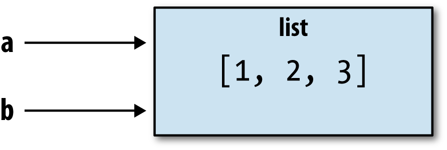
Figure 2-7. Two references for the same object
Understanding the semantics of references in Python and when, how, and why data is copied is especially critical when you are working with larger datasets in Python.
Note
Assignment is also referred to as binding, as we are binding a name to an object. Variable names that have been assigned may occasionally be referred to as bound variables.
When you pass objects as arguments to a function, new local variables are created referencing the original objects without any copying. If you bind a new object to a variable inside a function, that change will not be reflected in the parent scope. It is therefore possible to alter the internals of a mutable argument. Suppose we had the following function:
defappend_element(some_list,element):some_list.append(element)
Then we have:
In[27]:data=[1,2,3]In[28]:append_element(data,4)In[29]:dataOut[29]:[1,2,3,4]
Dynamic references, strong types
In contrast with many compiled languages, such as Java and C++, object references in Python have no type associated with them. There is no problem with the following:
In[12]:a=5In[13]:type(a)Out[13]:intIn[14]:a='foo'In[15]:type(a)Out[15]:str
Variables are names for objects within a particular namespace; the type information is stored in the object itself. Some observers might hastily conclude that Python is not a “typed language.” This is not true; consider this example:
In[16]:'5'+5---------------------------------------------------------------------------TypeErrorTraceback(mostrecentcalllast)<ipython-input-16-4dd8efb5fac1>in<module>()---->1'5'+5TypeError:mustbestr,notint
In some languages, such as Visual Basic, the string '5' might get implicitly converted (or
casted) to an integer, thus yielding 10. Yet in
other languages, such as JavaScript, the integer 5 might be casted to a string, yielding the
concatenated string '55'. In this
regard Python is considered a strongly typed
language, which means that every object has a specific type (or
class), and implicit conversions will occur only
in certain obvious circumstances, such as the following:
In[17]:a=4.5In[18]:b=2# String formatting, to be visited laterIn[19]:('a is {0}, b is {1}'.format(type(a),type(b)))ais<class'float'>, b is <class 'int'>In[20]:a/bOut[20]:2.25
Knowing the type of an object is important, and it’s useful to
be able to write functions that can handle many different kinds of
input. You can check that an object is an instance of a particular
type using the isinstance
function:
In[21]:a=5In[22]:isinstance(a,int)Out[22]:True
isinstance can accept a tuple
of types if you want to check that an object’s type is among those
present in the tuple:
In[23]:a=5;b=4.5In[24]:isinstance(a,(int,float))Out[24]:TrueIn[25]:isinstance(b,(int,float))Out[25]:True
Attributes and methods
Objects in Python typically have both attributes (other Python objects
stored “inside” the object) and methods (functions associated with an
object that can have access to the object’s internal data). Both of
them are accessed via the syntax
obj.attribute_name:
In[1]:a='foo'In[2]:a.<PressTab>a.capitalizea.formata.isuppera.rindexa.stripa.centera.indexa.joina.rjusta.swapcasea.counta.isalnuma.ljusta.rpartitiona.titlea.decodea.isalphaa.lowera.rsplita.translatea.encodea.isdigita.lstripa.rstripa.uppera.endswitha.islowera.partitiona.splita.zfilla.expandtabsa.isspacea.replacea.splitlinesa.finda.istitlea.rfinda.startswith
Attributes and methods can also be accessed by name via
the getattr
function:
In[27]:getattr(a,'split')Out[27]:<functionstr.split>
In other languages, accessing objects by name is often referred
to as “reflection.” While we will not extensively use the functions
getattr and related functions hasattr and
setattr in this book, they can be
used very effectively to write generic, reusable code.
Duck typing
Often you may not care about the type of an object but rather only whether it
has certain methods or behavior. This is sometimes called “duck
typing,” after the saying “If it walks like a duck and quacks like a
duck, then it’s a duck.” For example, you can verify that an object is
iterable if it implemented the iterator protocol. For many
objects, this means it has a __iter__
“magic method,” though an alternative and better way to check is to
try using the iter
function:
defisiterable(obj):try:iter(obj)returnTrueexceptTypeError:# not iterablereturnFalse
This function would return True for strings as well as most Python
collection types:
In[29]:isiterable('a string')Out[29]:TrueIn[30]:isiterable([1,2,3])Out[30]:TrueIn[31]:isiterable(5)Out[31]:False
A place where I use this functionality all the time is to write functions that can accept multiple kinds of input. A common case is writing a function that can accept any kind of sequence (list, tuple, ndarray) or even an iterator. You can first check if the object is a list (or a NumPy array) and, if it is not, convert it to be one:
ifnotisinstance(x,list)andisiterable(x):x=list(x)
Imports
In Python a module is simply a file with the .py extension containing Python code. Suppose that we had the following module:
# some_module.pyPI=3.14159deff(x):returnx+2defg(a,b):returna+b
If we wanted to access the variables and functions defined in some_module.py, from another file in the same directory we could do:
importsome_moduleresult=some_module.f(5)pi=some_module.PI
Or equivalently:
fromsome_moduleimportf,g,PIresult=g(5,PI)
By using the as keyword
you can give imports different variable names:
importsome_moduleassmfromsome_moduleimportPIaspi,gasgfr1=sm.f(pi)r2=gf(6,pi)
Binary operators and comparisons
Most of the binary math operations and comparisons are as you might expect:
In[32]:5-7Out[32]:-2In[33]:12+21.5Out[33]:33.5In[34]:5<=2Out[34]:False
See Table 2-3 for all of the available binary operators.
To check if two references refer to the same object, use the
is keyword. is not is also perfectly valid if you want
to check that two objects are not the same:
In[35]:a=[1,2,3]In[36]:b=aIn[37]:c=list(a)In[38]:aisbOut[38]:TrueIn[39]:aisnotcOut[39]:True
Since list always creates a new Python list (i.e., a copy), we can be sure
that c is distinct from a.
Comparing with is is not the same as the == operator, because in this case we
have:
In[40]:a==cOut[40]:True
A very common use of is and
is not is to check if a variable is
None, since there is only one
instance of None:
In[41]:a=NoneIn[42]:aisNoneOut[42]:True
Mutable and immutable objects
Most objects in Python, such as lists, dicts, NumPy arrays, and most user-defined types (classes), are mutable. This means that the object or values that they contain can be modified:
In[43]:a_list=['foo',2,[4,5]]In[44]:a_list[2]=(3,4)In[45]:a_listOut[45]:['foo',2,(3,4)]
Others, like strings and tuples, are immutable:
In[46]:a_tuple=(3,5,(4,5))In[47]:a_tuple[1]='four'---------------------------------------------------------------------------TypeErrorTraceback(mostrecentcalllast)<ipython-input-47-23fe12da1ba6>in<module>()---->1a_tuple[1]='four'TypeError:'tuple'objectdoesnotsupportitemassignment
Remember that just because you can mutate an object does not mean that you always should. Such actions are known as side effects. For example, when writing a function, any side effects should be explicitly communicated to the user in the function’s documentation or comments. If possible, I recommend trying to avoid side effects and favor immutability, even though there may be mutable objects involved.
Scalar Types
Python along with its standard library has a small set of built-in types for
handling numerical data, strings, boolean (True or False) values, and dates and time. These
“single value” types are sometimes called scalar
types and we refer to them in this book as scalars. See Table 2-4 for a list of the main scalar
types. Date and time handling will be discussed separately, as these are
provided by the datetime module in
the standard library.
Numeric types
The primary Python types for numbers are int and float. An int can store
arbitrarily large numbers:
In[48]:ival=17239871In[49]:ival**6Out[49]:26254519291092456596965462913230729701102721
Floating-point numbers are represented with the Python float type. Under the hood each one is a
double-precision (64-bit) value. They can also be expressed with
scientific notation:
In[50]:fval=7.243In[51]:fval2=6.78e-5
Integer division not resulting in a whole number will always yield a floating-point number:
In[52]:3/2Out[52]:1.5
To get C-style integer division (which drops the fractional part
if the result is not a whole number), use the floor division
operator //:
In[53]:3//2Out[53]:1
Strings
Many people use Python for its powerful and flexible built-in string
processing capabilities. You can write string
literals using either single quotes ' or double
quotes ":
a='one way of writing a string'b="another way"
For multiline strings with line breaks, you can use triple
quotes, either ''' or """:
c="""This is a longer string thatspans multiple lines"""
It may surprise you that this string c
actually contains four lines of text; the line breaks after
""" and after lines are included
in the string. We can count the new line characters with the count method on
c:
In[55]:c.count('\n')Out[55]:3
Python strings are immutable; you cannot modify a string:
In[56]:a='this is a string'In[57]:a[10]='f'---------------------------------------------------------------------------TypeErrorTraceback(mostrecentcalllast)<ipython-input-57-2151a30ed055>in<module>()---->1a[10]='f'TypeError:'str'objectdoesnotsupportitemassignmentIn[58]:b=a.replace('string','longer string')In[59]:bOut[59]:'this is a longer string'
Afer this operation, the variable a is
unmodified:
In[60]:aOut[60]:'this is a string'
Many Python objects can be converted to a string using the str
function:
In[61]:a=5.6In[62]:s=str(a)In[63]:(s)5.6
Strings are a sequence of Unicode characters and therefore can be treated like other sequences, such as lists and tuples (which we will explore in more detail in the next chapter):
In[64]:s='python'In[65]:list(s)Out[65]:['p','y','t','h','o','n']In[66]:s[:3]Out[66]:'pyt'
The syntax s[:3] is called
slicing and is implemented for many kinds of Python sequences.
This will be explained in more detail later on, as it is used
extensively in this book.
The backslash character \
is an escape character, meaning that it is used
to specify special characters like newline \n or Unicode characters. To write a string
literal with backslashes, you need to escape them:
In[67]:s='12\\34'In[68]:(s)12\34
If you have a string with a lot of backslashes and no special
characters, you might find this a bit annoying. Fortunately you can
preface the leading quote of the string with r, which
means that the characters should be interpreted as is:
In[69]:s=r'this\has\no\special\characters'In[70]:sOut[70]:'this\\has\\no\\special\\characters'
The r stands for
raw.
Adding two strings together concatenates them and produces a new string:
In[71]:a='this is the first half 'In[72]:b='and this is the second half'In[73]:a+bOut[73]:'this is the first half and this is the second half'
String templating or formatting is another important topic. The number of
ways to do so has expanded with the advent of Python 3, and here I will
briefly describe the mechanics of one of the main interfaces. String
objects have a format method that can be
used to substitute formatted arguments into the string, producing a
new string:
In[74]:template='{0:.2f} {1:s} are worth US${2:d}'
In this string,
{0:.2f}means to format the first argument as a floating-point number with two decimal places.{1:s}means to format the second argument as a string.{2:d}means to format the third argument as an exact integer.
To substitute arguments for these format parameters, we pass a
sequence of arguments to the format method:
In[75]:template.format(4.5560,'Argentine Pesos',1)Out[75]:'4.56 Argentine Pesos are worth US$1'
String formatting is a deep topic; there are multiple methods and numerous options and tweaks available to control how values are formatted in the resulting string. To learn more, I recommend consulting the official Python documentation.
I discuss general string processing as it relates to data analysis in more detail in Chapter 8.
Bytes and Unicode
In modern Python (i.e., Python 3.0 and up), Unicode has become the first-class string type to enable more consistent handling of ASCII and non-ASCII text. In older versions of Python, strings were all bytes without any explicit Unicode encoding. You could convert to Unicode assuming you knew the character encoding. Let’s look at an example:
In[76]:val="español"In[77]:valOut[77]:'español'
We can convert this Unicode string to its UTF-8 bytes
representation using the encode method:
In[78]:val_utf8=val.encode('utf-8')In[79]:val_utf8Out[79]:b'espa\xc3\xb1ol'In[80]:type(val_utf8)Out[80]:bytes
Assuming you know the Unicode encoding of a bytes object, you
can go back using the decode method:
In[81]:val_utf8.decode('utf-8')Out[81]:'español'
While it’s become preferred to use UTF-8 for any encoding, for historical reasons you may encounter data in any number of different encodings:
In[82]:val.encode('latin1')Out[82]:b'espa\xf1ol'In[83]:val.encode('utf-16')Out[83]:b'\xff\xfee\x00s\x00p\x00a\x00\xf1\x00o\x00l\x00'In[84]:val.encode('utf-16le')Out[84]:b'e\x00s\x00p\x00a\x00\xf1\x00o\x00l\x00'
It is most common to encounter bytes objects in the
context of working with files, where implicitly decoding all data to
Unicode strings may not be desired.
Though you may seldom need to do so, you can define your own
byte literals by prefixing a string with b:
In[85]:bytes_val=b'this is bytes'In[86]:bytes_valOut[86]:b'this is bytes'In[87]:decoded=bytes_val.decode('utf8')In[88]:decoded# this is str (Unicode) nowOut[88]:'this is bytes'
None
None is the Python null value type. If a function does not explicitly
return a value, it implicitly returns None:
In[97]:a=NoneIn[98]:aisNoneOut[98]:TrueIn[99]:b=5In[100]:bisnotNoneOut[100]:True
None is also a common default
value for function arguments:
defadd_and_maybe_multiply(a,b,c=None):result=a+bifcisnotNone:result=result*creturnresult
While a technical point, it’s worth bearing in mind that
None is not only a reserved keyword
but also a unique instance of NoneType:
In[101]:type(None)Out[101]:NoneType
Dates and times
The built-in Python datetime
module provides datetime,
date, and time types. The datetime type, as you may imagine, combines
the information stored in date and
time and is the most commonly
used:
In[102]:fromdatetimeimportdatetime,date,timeIn[103]:dt=datetime(2011,10,29,20,30,21)In[104]:dt.dayOut[104]:29In[105]:dt.minuteOut[105]:30
Given a datetime instance,
you can extract the equivalent date
and time objects by calling methods
on the datetime of the same
name:
In[106]:dt.date()Out[106]:datetime.date(2011,10,29)In[107]:dt.time()Out[107]:datetime.time(20,30,21)
The strftime method
formats a datetime as a
string:
In[108]:dt.strftime('%m/%d/%Y%H:%M')Out[108]:'10/29/2011 20:30'
Strings can be converted (parsed) into
datetime objects with the strptime
function:
In[109]:datetime.strptime('20091031','%Y%m%d')Out[109]:datetime.datetime(2009,10,31,0,0)
See Table 2-5 for a full list of format specifications.
When you are aggregating or otherwise grouping time series data, it will
occasionally be useful to replace time fields of a series of
datetimes—for example, replacing the minute and
second fields with zero:
In[110]:dt.replace(minute=0,second=0)Out[110]:datetime.datetime(2011,10,29,20,0)
Since datetime.datetime is an immutable type,
methods like these always produce new objects.
The difference of two datetime objects
produces a datetime.timedelta
type:
In[111]:dt2=datetime(2011,11,15,22,30)In[112]:delta=dt2-dtIn[113]:deltaOut[113]:datetime.timedelta(17,7179)In[114]:type(delta)Out[114]:datetime.timedelta
The output timedelta(17, 7179) indicates that
the timedelta encodes an offset of 17 days and 7,179 seconds.
Adding a timedelta to a
datetime produces a new shifted
datetime:
In[115]:dtOut[115]:datetime.datetime(2011,10,29,20,30,21)In[116]:dt+deltaOut[116]:datetime.datetime(2011,11,15,22,30)
Control Flow
Python has several built-in keywords for conditional logic, loops, and other standard control flow concepts found in other programming languages.
if, elif, and else
The if statement is one of the most well-known control flow statement
types. It checks a condition that, if True, evaluates the code in the block that
follows:
ifx<0:('It'snegative')
An if statement can be
optionally followed by one or more elif blocks and
a catch-all else block if all of the conditions are False:
ifx<0:('It'snegative')elifx==0:('Equal to zero')elif0<x<5:('Positive but smaller than 5')else:('Positive and larger than or equal to 5')
If any of the conditions is True, no further elif or else blocks will be reached. With a compound
condition using and or or, conditions are evaluated left to right
and will short-circuit:
In[117]:a=5;b=7In[118]:c=8;d=4In[119]:ifa<borc>d:.....:('Made it')Madeit
In this example, the comparison c >
d never gets evaluated because the first comparison was
True.
It is also possible to chain comparisons:
In[120]:4>3>2>1Out[120]:True
for loops
for loops are for iterating over a collection (like a list or tuple) or
an iterater. The standard syntax for a for loop is:
forvalueincollection:# do something with value
You can advance a for loop to
the next iteration, skipping the remainder of the block, using the
continue keyword. Consider this code, which sums up integers in a list and
skips None values:
sequence=[1,2,None,4,None,5]total=0forvalueinsequence:ifvalueisNone:continuetotal+=value
A for loop can be exited
altogether with the break keyword.
This code sums elements of the list until a 5 is reached:
sequence=[1,2,0,4,6,5,2,1]total_until_5=0forvalueinsequence:ifvalue==5:breaktotal_until_5+=value
The break keyword only terminates the
innermost for loop; any outer
for loops will continue to run:
In[121]:foriinrange(4):.....:forjinrange(4):.....:ifj>i:.....:break.....:((i,j)).....:(0,0)(1,0)(1,1)(2,0)(2,1)(2,2)(3,0)(3,1)(3,2)(3,3)
As we will see in more detail, if the elements in the collection
or iterator are sequences (tuples or lists, say), they can be
conveniently unpacked into variables in the
for loop statement:
fora,b,ciniterator:# do something
pass
pass is the “no-op” statement
in Python. It can be used in blocks where no action is
to be taken (or as a placeholder for code not yet implemented); it is
only required because Python uses whitespace to delimit blocks:
ifx<0:('negative!')elifx==0:# TODO: put something smart herepasselse:('positive!')
range
The range function returns an iterator that yields a sequence of evenly
spaced integers:
In[122]:range(10)Out[122]:range(0,10)In[123]:list(range(10))Out[123]:[0,1,2,3,4,5,6,7,8,9]
Both a start, end, and step (which may be negative) can be given:
In[124]:list(range(0,20,2))Out[124]:[0,2,4,6,8,10,12,14,16,18]In[125]:list(range(5,0,-1))Out[125]:[5,4,3,2,1]
As you can see, range
produces integers up to but not including the endpoint. A common use
of range is for iterating through
sequences by index:
seq=[1,2,3,4]foriinrange(len(seq)):val=seq[i]
While you can use functions like list to
store all the integers generated by range in some
other data structure, often the default iterator form will be what you
want. This snippet sums all numbers from 0 to 99,999 that are
multiples of 3 or 5:
sum=0foriinrange(100000):# % is the modulo operatorifi%3==0ori%5==0:sum+=i
While the range generated can be arbitrarily large, the memory use at any given time may be very small.
Ternary expressions
A ternary expression in Python allows you to combine an if-else block that produces a value into a
single line or expression. The syntax for this in Python is:
value =true-exprif condition elsefalse-expr
Here, true-expr and
false-expr can be any Python expressions.
It has the identical effect as the more verbose:
ifcondition: value =true-exprelse: value =false-expr
This is a more concrete example:
In[126]:x=5In[127]:'Non-negative'ifx>=0else'Negative'Out[127]:'Non-negative'
As with if-else blocks, only
one of the expressions will be executed. Thus, the “if” and “else”
sides of the ternary expression could contain costly computations, but
only the true branch is ever evaluated.
While it may be tempting to always use ternary expressions to condense your code, realize that you may sacrifice readability if the condition as well as the true and false expressions are very complex.