Chapter 10. Data Aggregation and Group Operations

Categorizing a dataset and applying a function to each group, whether an aggregation or transformation, is often a critical component of a data analysis workflow. After loading, merging, and preparing a dataset, you may need to compute group statistics or possibly pivot tables for reporting or visualization purposes. pandas provides a flexible groupby interface, enabling you to slice, dice, and summarize datasets in a natural way.

One reason for the popularity of relational databases and SQL (which stands for “structured query language”) is the ease with which data can be joined, filtered, transformed, and aggregated. However, query languages like SQL are somewhat constrained in the kinds of group operations that can be performed. As you will see, with the expressiveness of Python and pandas, we can perform quite complex group operations by utilizing any function that accepts a pandas object or NumPy array. In this chapter, you will learn how to:

Split a pandas object into pieces using one or more keys (in the form of functions, arrays, or DataFrame column names)
Calculate group summary statistics, like count, mean, or standard deviation, or a user-defined function
Apply within-group transformations or other manipulations, like normalization, linear regression, rank, or subset selection
Compute pivot tables and cross-tabulations
Perform quantile analysis and other statistical group analyses

Note

Aggregation of time series data, a special use case of groupby, is referred to as resampling in this book and will receive separate treatment in Chapter 11.

10.1 GroupBy Mechanics

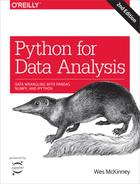
Hadley Wickham, an author of many popular packages for the R programming language, coined the term split-apply-combine for describing group operations. In the first stage of the process, data contained in a pandas object, whether a Series, DataFrame, or otherwise, is split into groups based on one or more keys that you provide. The splitting is performed on a particular axis of an object. For example, a DataFrame can be grouped on its rows (axis=0) or its columns (axis=1). Once this is done, a function is applied to each group, producing a new value. Finally, the results of all those function applications are combined into a result object. The form of the resulting object will usually depend on what’s being done to the data. See Figure 10-1 for a mockup of a simple group aggregation.

Each grouping key can take many forms, and the keys do not have to be all of the same type:

A list or array of values that is the same length as the axis being grouped
A value indicating a column name in a DataFrame
A dict or Series giving a correspondence between the values on the axis being grouped and the group names
A function to be invoked on the axis index or the individual labels in the index

Note that the latter three methods are shortcuts for producing an array of values to be used to split up the object. Don’t worry if this all seems abstract. Throughout this chapter, I will give many examples of all these methods. To get started, here is a small tabular dataset as a DataFrame:

In [10]: df = pd.DataFrame({'key1' : ['a', 'a', 'b', 'b', 'a'],
   ....:                    'key2' : ['one', 'two', 'one', 'two', 'one'],
   ....:                    'data1' : np.random.randn(5),
   ....:                    'data2' : np.random.randn(5)})

In [11]: df
Out[11]: 
      data1     data2 key1 key2
0 -0.204708  1.393406    a  one
1  0.478943  0.092908    a  two
2 -0.519439  0.281746    b  one
3 -0.555730  0.769023    b  two
4  1.965781  1.246435    a  one

Suppose you wanted to compute the mean of the data1 column using the labels from key1. There are a number of ways to do this. One is to access data1 and call groupby with the column (a Series) at key1:

In [12]: grouped = df['data1'].groupby(df['key1'])

In [13]: grouped
Out[13]: <pandas.core.groupby.SeriesGroupBy object at 0x7f85008d0400>

This grouped variable is now a GroupBy object. It has not actually computed anything yet except for some intermediate data about the group key df['key1']. The idea is that this object has all of the information needed to then apply some operation to each of the groups. For example, to compute group means we can call the GroupBy’s mean method:

In [14]: grouped.mean()
Out[14]: 
key1
a    0.746672
b   -0.537585
Name: data1, dtype: float64

Later, I’ll explain more about what happens when you call .mean(). The important thing here is that the data (a Series) has been aggregated according to the group key, producing a new Series that is now indexed by the unique values in the key1 column. The result index has the name 'key1' because the DataFrame column df['key1'] did.

If instead we had passed multiple arrays as a list, we’d get something different:

In [15]: means = df['data1'].groupby([df['key1'], df['key2']]).mean()

In [16]: means
Out[16]: 
key1  key2
a     one     0.880536
      two     0.478943
b     one    -0.519439
      two    -0.555730
Name: data1, dtype: float64

Here we grouped the data using two keys, and the resulting Series now has a hierarchical index consisting of the unique pairs of keys observed:

In [17]: means.unstack()
Out[17]: 
key2       one       two
key1                    
a     0.880536  0.478943
b    -0.519439 -0.555730

In this example, the group keys are all Series, though they could be any arrays of the right length:

In [18]: states = np.array(['Ohio', 'California', 'California', 'Ohio', 'Ohio'])

In [19]: years = np.array([2005, 2005, 2006, 2005, 2006])

In [20]: df['data1'].groupby([states, years]).mean()
Out[20]: 
California  2005    0.478943
            2006   -0.519439
Ohio        2005   -0.380219
            2006    1.965781
Name: data1, dtype: float64

Frequently the grouping information is found in the same DataFrame as the data you want to work on. In that case, you can pass column names (whether those are strings, numbers, or other Python objects) as the group keys:

In [21]: df.groupby('key1').mean()
Out[21]: 
         data1     data2
key1                    
a     0.746672  0.910916
b    -0.537585  0.525384

In [22]: df.groupby(['key1', 'key2']).mean()
Out[22]: 
              data1     data2
key1 key2                    
a    one   0.880536  1.319920
     two   0.478943  0.092908
b    one  -0.519439  0.281746
     two  -0.555730  0.769023

You may have noticed in the first case df.groupby('key1').mean() that there is no key2 column in the result. Because df['key2'] is not numeric data, it is said to be a nuisance column, which is therefore excluded from the result. By default, all of the numeric columns are aggregated, though it is possible to filter down to a subset, as you’ll see soon.

Regardless of the objective in using groupby, a generally useful GroupBy method is size, which returns a Series containing group sizes:

In [23]: df.groupby(['key1', 'key2']).size()
Out[23]: 
key1  key2
a     one     2
      two     1
b     one     1
      two     1
dtype: int64

Take note that any missing values in a group key will be excluded from the result.

Iterating Over Groups

The GroupBy object supports iteration, generating a sequence of 2-tuples containing the group name along with the chunk of data. Consider the following:

In [24]: for name, group in df.groupby('key1'):
   ....:     print(name)
   ....:     print(group)
   ....:
a
      data1     data2 key1 key2
0 -0.204708  1.393406    a  one
1  0.478943  0.092908    a  two
4  1.965781  1.246435    a  one
b
      data1     data2 key1 key2
2 -0.519439  0.281746    b  one
3 -0.555730  0.769023    b  two

In the case of multiple keys, the first element in the tuple will be a tuple of key values:

In [25]: for (k1, k2), group in df.groupby(['key1', 'key2']):
   ....:     print((k1, k2))
   ....:     print(group)
   ....:
('a', 'one')
      data1     data2 key1 key2
0 -0.204708  1.393406    a  one
4  1.965781  1.246435    a  one
('a', 'two')
      data1     data2 key1 key2
1  0.478943  0.092908    a  two
('b', 'one')
      data1     data2 key1 key2
2 -0.519439  0.281746    b  one
('b', 'two')
     data1     data2 key1 key2
3 -0.55573  0.769023    b  two

Of course, you can choose to do whatever you want with the pieces of data. A recipe you may find useful is computing a dict of the data pieces as a one-liner:

In [26]: pieces = dict(list(df.groupby('key1')))

In [27]: pieces['b']
Out[27]: 
      data1     data2 key1 key2
2 -0.519439  0.281746    b  one
3 -0.555730  0.769023    b  two

By default groupby groups on axis=0, but you can group on any of the other axes. For example, we could group the columns of our example df here by dtype like so:

In [28]: df.dtypes
Out[28]: 
data1    float64
data2    float64
key1      object
key2      object
dtype: object

In [29]: grouped = df.groupby(df.dtypes, axis=1)

We can print out the groups like so:

In [30]: for dtype, group in grouped:
   ....:     print(dtype)
   ....:     print(group)
   ....:
float64
      data1     data2
0 -0.204708  1.393406
1  0.478943  0.092908
2 -0.519439  0.281746
3 -0.555730  0.769023
4  1.965781  1.246435
object
  key1 key2
0    a  one
1    a  two
2    b  one
3    b  two
4    a  one

Selecting a Column or Subset of Columns

Indexing a GroupBy object created from a DataFrame with a column name or array of column names has the effect of column subsetting for aggregation. This means that:

df.groupby('key1')['data1']
df.groupby('key1')[['data2']]

are syntactic sugar for:

df['data1'].groupby(df['key1'])
df[['data2']].groupby(df['key1'])

Especially for large datasets, it may be desirable to aggregate only a few columns. For example, in the preceding dataset, to compute means for just the data2 column and get the result as a DataFrame, we could write:

In [31]: df.groupby(['key1', 'key2'])[['data2']].mean()
Out[31]: 
              data2
key1 key2          
a    one   1.319920
     two   0.092908
b    one   0.281746
     two   0.769023

The object returned by this indexing operation is a grouped DataFrame if a list or array is passed or a grouped Series if only a single column name is passed as a scalar:

In [32]: s_grouped = df.groupby(['key1', 'key2'])['data2']

In [33]: s_grouped
Out[33]: <pandas.core.groupby.SeriesGroupBy object at 0x7f85008983c8>

In [34]: s_grouped.mean()
Out[34]: 
key1  key2
a     one     1.319920
      two     0.092908
b     one     0.281746
      two     0.769023
Name: data2, dtype: float64

Grouping with Dicts and Series

Grouping information may exist in a form other than an array. Let’s consider another example DataFrame:

In [35]: people = pd.DataFrame(np.random.randn(5, 5),
   ....:                       columns=['a', 'b', 'c', 'd', 'e'],
   ....:                       index=['Joe', 'Steve', 'Wes', 'Jim', 'Travis'])

In [36]: people.iloc[2:3, [1, 2]] = np.nan # Add a few NA values

In [37]: people
Out[37]: 
               a         b         c         d         e
Joe     1.007189 -1.296221  0.274992  0.228913  1.352917
Steve   0.886429 -2.001637 -0.371843  1.669025 -0.438570
Wes    -0.539741       NaN       NaN -1.021228 -0.577087
Jim     0.124121  0.302614  0.523772  0.000940  1.343810
Travis -0.713544 -0.831154 -2.370232 -1.860761 -0.860757

Now, suppose I have a group correspondence for the columns and want to sum together the columns by group:

In [38]: mapping = {'a': 'red', 'b': 'red', 'c': 'blue',
   ....:            'd': 'blue', 'e': 'red', 'f' : 'orange'}

Now, you could construct an array from this dict to pass to groupby, but instead we can just pass the dict (I included the key 'f' to highlight that unused grouping keys are OK):

In [39]: by_column = people.groupby(mapping, axis=1)

In [40]: by_column.sum()
Out[40]: 
            blue       red
Joe     0.503905  1.063885
Steve   1.297183 -1.553778
Wes    -1.021228 -1.116829
Jim     0.524712  1.770545
Travis -4.230992 -2.405455

The same functionality holds for Series, which can be viewed as a fixed-size mapping:

In [41]: map_series = pd.Series(mapping)

In [42]: map_series
Out[42]: 
a       red
b       red
c      blue
d      blue
e       red
f    orange
dtype: object

In [43]: people.groupby(map_series, axis=1).count()
Out[43]: 
        blue  red
Joe        2    3
Steve      2    3
Wes        1    2
Jim        2    3
Travis     2    3

Grouping with Functions

Using Python functions is a more generic way of defining a group mapping compared with a dict or Series. Any function passed as a group key will be called once per index value, with the return values being used as the group names. More concretely, consider the example DataFrame from the previous section, which has people’s first names as index values. Suppose you wanted to group by the length of the names; while you could compute an array of string lengths, it’s simpler to just pass the len function:

In [44]: people.groupby(len).sum()
Out[44]: 
          a         b         c         d         e
3  0.591569 -0.993608  0.798764 -0.791374  2.119639
5  0.886429 -2.001637 -0.371843  1.669025 -0.438570
6 -0.713544 -0.831154 -2.370232 -1.860761 -0.860757

Mixing functions with arrays, dicts, or Series is not a problem as everything gets converted to arrays internally:

In [45]: key_list = ['one', 'one', 'one', 'two', 'two']

In [46]: people.groupby([len, key_list]).min()
Out[46]: 
              a         b         c         d         e
3 one -0.539741 -1.296221  0.274992 -1.021228 -0.577087
  two  0.124121  0.302614  0.523772  0.000940  1.343810
5 one  0.886429 -2.001637 -0.371843  1.669025 -0.438570
6 two -0.713544 -0.831154 -2.370232 -1.860761 -0.860757

Grouping by Index Levels

A final convenience for hierarchically indexed datasets is the ability to aggregate using one of the levels of an axis index. Let’s look at an example:

In [47]: columns = pd.MultiIndex.from_arrays([['US', 'US', 'US', 'JP', 'JP'],
   ....:                                     [1, 3, 5, 1, 3]],
   ....:                                     names=['cty', 'tenor'])

In [48]: hier_df = pd.DataFrame(np.random.randn(4, 5), columns=columns)

In [49]: hier_df
Out[49]: 
cty          US                            JP          
tenor         1         3         5         1         3
0      0.560145 -1.265934  0.119827 -1.063512  0.332883
1     -2.359419 -0.199543 -1.541996 -0.970736 -1.307030
2      0.286350  0.377984 -0.753887  0.331286  1.349742
3      0.069877  0.246674 -0.011862  1.004812  1.327195

To group by level, pass the level number or name using the level keyword:

In [50]: hier_df.groupby(level='cty', axis=1).count()
Out[50]: 
cty  JP  US
0     2   3
1     2   3
2     2   3
3     2   3

10.2 Data Aggregation

Aggregations refer to any data transformation that produces scalar values from arrays. The preceding examples have used several of them, including mean, count, min, and sum. You may wonder what is going on when you invoke mean() on a GroupBy object. Many common aggregations, such as those found in Table 10-1, have optimized implementations. However, you are not limited to only this set of methods.

Table 10-1. Optimized groupby methods
Function name	Description
`count`	Number of non-NA values in the group
`sum`	Sum of non-NA values
`mean`	Mean of non-NA values
`median`	Arithmetic median of non-NA values
`std, var`	Unbiased (n – 1 denominator) standard deviation and variance
`min, max`	Minimum and maximum of non-NA values
`prod`	Product of non-NA values
`first, last`	First and last non-NA values

You can use aggregations of your own devising and additionally call any method that is also defined on the grouped object. For example, you might recall that quantile computes sample quantiles of a Series or a DataFrame’s columns.

While quantile is not explicitly implemented for GroupBy, it is a Series method and thus available for use. Internally, GroupBy efficiently slices up the Series, calls piece.quantile(0.9) for each piece, and then assembles those results together into the result object:

In [51]: df
Out[51]: 
      data1     data2 key1 key2
0 -0.204708  1.393406    a  one
1  0.478943  0.092908    a  two
2 -0.519439  0.281746    b  one
3 -0.555730  0.769023    b  two
4  1.965781  1.246435    a  one

In [52]: grouped = df.groupby('key1')

In [53]: grouped['data1'].quantile(0.9)
Out[53]: 
key1
a    1.668413
b   -0.523068
Name: data1, dtype: float64

To use your own aggregation functions, pass any function that aggregates an array to the aggregate or agg method:

In [54]: def peak_to_peak(arr):
   ....:     return arr.max() - arr.min()

In [55]: grouped.agg(peak_to_peak)
Out[55]: 
         data1     data2
key1                    
a     2.170488  1.300498
b     0.036292  0.487276

You may notice that some methods like describe also work, even though they are not aggregations, strictly speaking:

In [56]: grouped.describe()
Out[56]: 
     data1                                                              \
     count      mean       std       min       25%       50%       75%   
key1                                                                     
a      3.0  0.746672  1.109736 -0.204708  0.137118  0.478943  1.222362   
b      2.0 -0.537585  0.025662 -0.555730 -0.546657 -0.537585 -0.528512   
               data2                                                    \
           max count      mean       std       min       25%       50%   
key1                                                                     
a     1.965781   3.0  0.910916  0.712217  0.092908  0.669671  1.246435   
b    -0.519439   2.0  0.525384  0.344556  0.281746  0.403565  0.525384   
                          
           75%       max  
key1                      
a     1.319920  1.393406  
b     0.647203  0.769023

I will explain in more detail what has happened here in Section 10.3, “Apply: General split-apply-combine,”.

Note

Custom aggregation functions are generally much slower than the optimized functions found in Table 10-1. This is because there is some extra overhead (function calls, data rearrangement) in constructing the intermediate group data chunks.

Column-Wise and Multiple Function Application

Let’s return to the tipping dataset from earlier examples. After loading it with read_csv, we add a tipping percentage column tip_pct:

In [57]: tips = pd.read_csv('examples/tips.csv')

# Add tip percentage of total bill
In [58]: tips['tip_pct'] = tips['tip'] / tips['total_bill']

In [59]: tips[:6]
Out[59]: 
   total_bill   tip smoker  day    time  size   tip_pct
0       16.99  1.01     No  Sun  Dinner     2  0.059447
1       10.34  1.66     No  Sun  Dinner     3  0.160542
2       21.01  3.50     No  Sun  Dinner     3  0.166587
3       23.68  3.31     No  Sun  Dinner     2  0.139780
4       24.59  3.61     No  Sun  Dinner     4  0.146808
5       25.29  4.71     No  Sun  Dinner     4  0.186240

As you’ve already seen, aggregating a Series or all of the columns of a DataFrame is a matter of using aggregate with the desired function or calling a method like mean or std. However, you may want to aggregate using a different function depending on the column, or multiple functions at once. Fortunately, this is possible to do, which I’ll illustrate through a number of examples. First, I’ll group the tips by day and smoker:

In [60]: grouped = tips.groupby(['day', 'smoker'])

Note that for descriptive statistics like those in Table 10-1, you can pass the name of the function as a string:

In [61]: grouped_pct = grouped['tip_pct']

In [62]: grouped_pct.agg('mean')
Out[62]: 
day   smoker
Fri   No        0.151650
      Yes       0.174783
Sat   No        0.158048
      Yes       0.147906
Sun   No        0.160113
      Yes       0.187250
Thur  No        0.160298
      Yes       0.163863
Name: tip_pct, dtype: float64

If you pass a list of functions or function names instead, you get back a DataFrame with column names taken from the functions:

In [63]: grouped_pct.agg(['mean', 'std', peak_to_peak])
Out[63]: 
                 mean       std  peak_to_peak
day  smoker                                  
Fri  No      0.151650  0.028123      0.067349
     Yes     0.174783  0.051293      0.159925
Sat  No      0.158048  0.039767      0.235193
     Yes     0.147906  0.061375      0.290095
Sun  No      0.160113  0.042347      0.193226
     Yes     0.187250  0.154134      0.644685
Thur No      0.160298  0.038774      0.193350
     Yes     0.163863  0.039389      0.151240

Here we passed a list of aggregation functions to agg to evaluate indepedently on the data groups.

You don’t need to accept the names that GroupBy gives to the columns; notably, lambda functions have the name '<lambda>', which makes them hard to identify (you can see for yourself by looking at a function’s __name__ attribute). Thus, if you pass a list of (name, function) tuples, the first element of each tuple will be used as the DataFrame column names (you can think of a list of 2-tuples as an ordered mapping):

In [64]: grouped_pct.agg([('foo', 'mean'), ('bar', np.std)])
Out[64]: 
                  foo       bar
day  smoker                    
Fri  No      0.151650  0.028123
     Yes     0.174783  0.051293
Sat  No      0.158048  0.039767
     Yes     0.147906  0.061375
Sun  No      0.160113  0.042347
     Yes     0.187250  0.154134
Thur No      0.160298  0.038774
     Yes     0.163863  0.039389

With a DataFrame you have more options, as you can specify a list of functions to apply to all of the columns or different functions per column. To start, suppose we wanted to compute the same three statistics for the tip_pct and total_bill columns:

In [65]: functions = ['count', 'mean', 'max']

In [66]: result = grouped['tip_pct', 'total_bill'].agg(functions)

In [67]: result
Out[67]: 
            tip_pct                     total_bill                  
              count      mean       max      count       mean    max
day  smoker                                                         
Fri  No           4  0.151650  0.187735          4  18.420000  22.75
     Yes         15  0.174783  0.263480         15  16.813333  40.17
Sat  No          45  0.158048  0.291990         45  19.661778  48.33
     Yes         42  0.147906  0.325733         42  21.276667  50.81
Sun  No          57  0.160113  0.252672         57  20.506667  48.17
     Yes         19  0.187250  0.710345         19  24.120000  45.35
Thur No          45  0.160298  0.266312         45  17.113111  41.19
     Yes         17  0.163863  0.241255         17  19.190588  43.11

As you can see, the resulting DataFrame has hierarchical columns, the same as you would get aggregating each column separately and using concat to glue the results together using the column names as the keys argument:

In [68]: result['tip_pct']
Out[68]: 
             count      mean       max
day  smoker                           
Fri  No          4  0.151650  0.187735
     Yes        15  0.174783  0.263480
Sat  No         45  0.158048  0.291990
     Yes        42  0.147906  0.325733
Sun  No         57  0.160113  0.252672
     Yes        19  0.187250  0.710345
Thur No         45  0.160298  0.266312
     Yes        17  0.163863  0.241255

As before, a list of tuples with custom names can be passed:

In [69]: ftuples = [('Durchschnitt', 'mean'), ('Abweichung', np.var)]

In [70]: grouped['tip_pct', 'total_bill'].agg(ftuples)
Out[70]: 
                 tip_pct              total_bill            
            Durchschnitt Abweichung Durchschnitt  Abweichung
day  smoker                                                 
Fri  No         0.151650   0.000791    18.420000   25.596333
     Yes        0.174783   0.002631    16.813333   82.562438
Sat  No         0.158048   0.001581    19.661778   79.908965
     Yes        0.147906   0.003767    21.276667  101.387535
Sun  No         0.160113   0.001793    20.506667   66.099980
     Yes        0.187250   0.023757    24.120000  109.046044
Thur No         0.160298   0.001503    17.113111   59.625081
     Yes        0.163863   0.001551    19.190588   69.808518

Now, suppose you wanted to apply potentially different functions to one or more of the columns. To do this, pass a dict to agg that contains a mapping of column names to any of the function specifications listed so far:

In [71]: grouped.agg({'tip' : np.max, 'size' : 'sum'})
Out[71]: 
               tip  size
day  smoker             
Fri  No       3.50     9
     Yes      4.73    31
Sat  No       9.00   115
     Yes     10.00   104
Sun  No       6.00   167
     Yes      6.50    49
Thur No       6.70   112
     Yes      5.00    40

In [72]: grouped.agg({'tip_pct' : ['min', 'max', 'mean', 'std'],
   ....:              'size' : 'sum'})
Out[72]: 
              tip_pct                               size
                  min       max      mean       std  sum
day  smoker                                             
Fri  No      0.120385  0.187735  0.151650  0.028123    9
     Yes     0.103555  0.263480  0.174783  0.051293   31
Sat  No      0.056797  0.291990  0.158048  0.039767  115
     Yes     0.035638  0.325733  0.147906  0.061375  104
Sun  No      0.059447  0.252672  0.160113  0.042347  167
     Yes     0.065660  0.710345  0.187250  0.154134   49
Thur No      0.072961  0.266312  0.160298  0.038774  112
     Yes     0.090014  0.241255  0.163863  0.039389   40

A DataFrame will have hierarchical columns only if multiple functions are applied to at least one column.

Returning Aggregated Data Without Row Indexes

In all of the examples up until now, the aggregated data comes back with an index, potentially hierarchical, composed from the unique group key combinations. Since this isn’t always desirable, you can disable this behavior in most cases by passing as_index=False to groupby:

In [73]: tips.groupby(['day', 'smoker'], as_index=False).mean()
Out[73]: 
    day smoker  total_bill       tip      size   tip_pct
0   Fri     No   18.420000  2.812500  2.250000  0.151650
1   Fri    Yes   16.813333  2.714000  2.066667  0.174783
2   Sat     No   19.661778  3.102889  2.555556  0.158048
3   Sat    Yes   21.276667  2.875476  2.476190  0.147906
4   Sun     No   20.506667  3.167895  2.929825  0.160113
5   Sun    Yes   24.120000  3.516842  2.578947  0.187250
6  Thur     No   17.113111  2.673778  2.488889  0.160298
7  Thur    Yes   19.190588  3.030000  2.352941  0.163863

Of course, it’s always possible to obtain the result in this format by calling reset_index on the result. Using the as_index=False method avoids some unnecessary computations.

10.3 Apply: General split-apply-combine

The most general-purpose GroupBy method is apply, which is the subject of the rest of this section. As illustrated in Figure 10-2, apply splits the object being manipulated into pieces, invokes the passed function on each piece, and then attempts to concatenate the pieces together.

Returning to the tipping dataset from before, suppose you wanted to select the top five tip_pct values by group. First, write a function that selects the rows with the largest values in a particular column:

In [74]: def top(df, n=5, column='tip_pct'):
   ....:     return df.sort_values(by=column)[-n:]

In [75]: top(tips, n=6)
Out[75]: 
     total_bill   tip smoker  day    time  size   tip_pct
109       14.31  4.00    Yes  Sat  Dinner     2  0.279525
183       23.17  6.50    Yes  Sun  Dinner     4  0.280535
232       11.61  3.39     No  Sat  Dinner     2  0.291990
67         3.07  1.00    Yes  Sat  Dinner     1  0.325733
178        9.60  4.00    Yes  Sun  Dinner     2  0.416667
172        7.25  5.15    Yes  Sun  Dinner     2  0.710345

Now, if we group by smoker, say, and call apply with this function, we get the following:

In [76]: tips.groupby('smoker').apply(top)
Out[76]: 
            total_bill   tip smoker   day    time  size   tip_pct
smoker                                                           
No     88        24.71  5.85     No  Thur   Lunch     2  0.236746
       185       20.69  5.00     No   Sun  Dinner     5  0.241663
       51        10.29  2.60     No   Sun  Dinner     2  0.252672
       149        7.51  2.00     No  Thur   Lunch     2  0.266312
       232       11.61  3.39     No   Sat  Dinner     2  0.291990
Yes    109       14.31  4.00    Yes   Sat  Dinner     2  0.279525
       183       23.17  6.50    Yes   Sun  Dinner     4  0.280535
       67         3.07  1.00    Yes   Sat  Dinner     1  0.325733
       178        9.60  4.00    Yes   Sun  Dinner     2  0.416667
       172        7.25  5.15    Yes   Sun  Dinner     2  0.710345

What has happened here? The top function is called on each row group from the DataFrame, and then the results are glued together using pandas.concat, labeling the pieces with the group names. The result therefore has a hierarchical index whose inner level contains index values from the original DataFrame.

If you pass a function to apply that takes other arguments or keywords, you can pass these after the function:

In [77]: tips.groupby(['smoker', 'day']).apply(top, n=1, column='total_bill')
Out[77]: 
                 total_bill    tip smoker   day    time  size   tip_pct
smoker day                                                             
No     Fri  94        22.75   3.25     No   Fri  Dinner     2  0.142857
       Sat  212       48.33   9.00     No   Sat  Dinner     4  0.186220
       Sun  156       48.17   5.00     No   Sun  Dinner     6  0.103799
       Thur 142       41.19   5.00     No  Thur   Lunch     5  0.121389
Yes    Fri  95        40.17   4.73    Yes   Fri  Dinner     4  0.117750
       Sat  170       50.81  10.00    Yes   Sat  Dinner     3  0.196812
       Sun  182       45.35   3.50    Yes   Sun  Dinner     3  0.077178
       Thur 197       43.11   5.00    Yes  Thur   Lunch     4  0.115982

Note

Beyond these basic usage mechanics, getting the most out of apply may require some creativity. What occurs inside the function passed is up to you; it only needs to return a pandas object or a scalar value. The rest of this chapter will mainly consist of examples showing you how to solve various problems using groupby.

You may recall that I earlier called describe on a GroupBy object:

In [78]: result = tips.groupby('smoker')['tip_pct'].describe()

In [79]: result
Out[79]: 
        count      mean       std       min       25%       50%       75%  \
smoker                                                                      
No      151.0  0.159328  0.039910  0.056797  0.136906  0.155625  0.185014   
Yes      93.0  0.163196  0.085119  0.035638  0.106771  0.153846  0.195059   
             max  
smoker            
No      0.291990  
Yes     0.710345  

In [80]: result.unstack('smoker')
Out[80]: 
       smoker
count  No        151.000000
       Yes        93.000000
mean   No          0.159328
       Yes         0.163196
std    No          0.039910
       Yes         0.085119
min    No          0.056797
       Yes         0.035638
25%    No          0.136906
       Yes         0.106771
50%    No          0.155625
       Yes         0.153846
75%    No          0.185014
       Yes         0.195059
max    No          0.291990
       Yes         0.710345
dtype: float64

Inside GroupBy, when you invoke a method like describe, it is actually just a shortcut for:

f = lambda x: x.describe()
grouped.apply(f)

Suppressing the Group Keys

In the preceding examples, you see that the resulting object has a hierarchical index formed from the group keys along with the indexes of each piece of the original object. You can disable this by passing group_keys=False to groupby:

In [81]: tips.groupby('smoker', group_keys=False).apply(top)
Out[81]: 
     total_bill   tip smoker   day    time  size   tip_pct
88        24.71  5.85     No  Thur   Lunch     2  0.236746
185       20.69  5.00     No   Sun  Dinner     5  0.241663
51        10.29  2.60     No   Sun  Dinner     2  0.252672
149        7.51  2.00     No  Thur   Lunch     2  0.266312
232       11.61  3.39     No   Sat  Dinner     2  0.291990
109       14.31  4.00    Yes   Sat  Dinner     2  0.279525
183       23.17  6.50    Yes   Sun  Dinner     4  0.280535
67         3.07  1.00    Yes   Sat  Dinner     1  0.325733
178        9.60  4.00    Yes   Sun  Dinner     2  0.416667
172        7.25  5.15    Yes   Sun  Dinner     2  0.710345

Quantile and Bucket Analysis

As you may recall from Chapter 8, pandas has some tools, in particular cut and qcut, for slicing data up into buckets with bins of your choosing or by sample quantiles. Combining these functions with groupby makes it convenient to perform bucket or quantile analysis on a dataset. Consider a simple random dataset and an equal-length bucket categorization using cut:

In [82]: frame = pd.DataFrame({'data1': np.random.randn(1000),
   ....:                       'data2': np.random.randn(1000)})

In [83]: quartiles = pd.cut(frame.data1, 4)

In [84]: quartiles[:10]
Out[84]: 
0     (-1.23, 0.489]
1    (-2.956, -1.23]
2     (-1.23, 0.489]
3     (0.489, 2.208]
4     (-1.23, 0.489]
5     (0.489, 2.208]
6     (-1.23, 0.489]
7     (-1.23, 0.489]
8     (0.489, 2.208]
9     (0.489, 2.208]
Name: data1, dtype: category
Categories (4, interval[float64]): [(-2.956, -1.23] < (-1.23, 0.489] < (0.489, 2.
208] < (2.208, 3.928]]

The Categorical object returned by cut can be passed directly to groupby. So we could compute a set of statistics for the data2 column like so:

In [85]: def get_stats(group):
   ....:     return {'min': group.min(), 'max': group.max(),
   ....:             'count': group.count(), 'mean': group.mean()}

In [86]: grouped = frame.data2.groupby(quartiles)

In [87]: grouped.apply(get_stats).unstack()
Out[87]: 
                 count       max      mean       min
data1                                               
(-2.956, -1.23]   95.0  1.670835 -0.039521 -3.399312
(-1.23, 0.489]   598.0  3.260383 -0.002051 -2.989741
(0.489, 2.208]   297.0  2.954439  0.081822 -3.745356
(2.208, 3.928]    10.0  1.765640  0.024750 -1.929776

These were equal-length buckets; to compute equal-size buckets based on sample quantiles, use qcut. I’ll pass labels=False to just get quantile numbers:

# Return quantile numbers
In [88]: grouping = pd.qcut(frame.data1, 10, labels=False)

In [89]: grouped = frame.data2.groupby(grouping)

In [90]: grouped.apply(get_stats).unstack()
Out[90]: 
       count       max      mean       min
data1                                     
0      100.0  1.670835 -0.049902 -3.399312
1      100.0  2.628441  0.030989 -1.950098
2      100.0  2.527939 -0.067179 -2.925113
3      100.0  3.260383  0.065713 -2.315555
4      100.0  2.074345 -0.111653 -2.047939
5      100.0  2.184810  0.052130 -2.989741
6      100.0  2.458842 -0.021489 -2.223506
7      100.0  2.954439 -0.026459 -3.056990
8      100.0  2.735527  0.103406 -3.745356
9      100.0  2.377020  0.220122 -2.064111

We will take a closer look at pandas’s Categorical type in Chapter 12.

Example: Filling Missing Values with Group-Specific Values

When cleaning up missing data, in some cases you will replace data observations using dropna, but in others you may want to impute (fill in) the null (NA) values using a fixed value or some value derived from the data. fillna is the right tool to use; for example, here I fill in NA values with the mean:

In [91]: s = pd.Series(np.random.randn(6))

In [92]: s[::2] = np.nan

In [93]: s
Out[93]: 
0         NaN
1   -0.125921
2         NaN
3   -0.884475
4         NaN
5    0.227290
dtype: float64

In [94]: s.fillna(s.mean())
Out[94]: 
0   -0.261035
1   -0.125921
2   -0.261035
3   -0.884475
4   -0.261035
5    0.227290
dtype: float64

Suppose you need the fill value to vary by group. One way to do this is to group the data and use apply with a function that calls fillna on each data chunk. Here is some sample data on US states divided into eastern and western regions:

In [95]: states = ['Ohio', 'New York', 'Vermont', 'Florida',
   ....:           'Oregon', 'Nevada', 'California', 'Idaho']

In [96]: group_key = ['East'] * 4 + ['West'] * 4

In [97]: data = pd.Series(np.random.randn(8), index=states)

In [98]: data
Out[98]: 
Ohio          0.922264
New York     -2.153545
Vermont      -0.365757
Florida      -0.375842
Oregon        0.329939
Nevada        0.981994
California    1.105913
Idaho        -1.613716
dtype: float64

Note that the syntax ['East'] * 4 produces a list containing four copies of the elements in ['East']. Adding lists together concatenates them.

Let’s set some values in the data to be missing:

In [99]: data[['Vermont', 'Nevada', 'Idaho']] = np.nan

In [100]: data
Out[100]: 
Ohio          0.922264
New York     -2.153545
Vermont            NaN
Florida      -0.375842
Oregon        0.329939
Nevada             NaN
California    1.105913
Idaho              NaN
dtype: float64

In [101]: data.groupby(group_key).mean()
Out[101]: 
East   -0.535707
West    0.717926
dtype: float64

We can fill the NA values using the group means like so:

In [102]: fill_mean = lambda g: g.fillna(g.mean())

In [103]: data.groupby(group_key).apply(fill_mean)
Out[103]: 
Ohio          0.922264
New York     -2.153545
Vermont      -0.535707
Florida      -0.375842
Oregon        0.329939
Nevada        0.717926
California    1.105913
Idaho         0.717926
dtype: float64

In another case, you might have predefined fill values in your code that vary by group. Since the groups have a name attribute set internally, we can use that:

In [104]: fill_values = {'East': 0.5, 'West': -1}

In [105]: fill_func = lambda g: g.fillna(fill_values[g.name])

In [106]: data.groupby(group_key).apply(fill_func)
Out[106]: 
Ohio          0.922264
New York     -2.153545
Vermont       0.500000
Florida      -0.375842
Oregon        0.329939
Nevada       -1.000000
California    1.105913
Idaho        -1.000000
dtype: float64

Example: Random Sampling and Permutation

Suppose you wanted to draw a random sample (with or without replacement) from a large dataset for Monte Carlo simulation purposes or some other application. There are a number of ways to perform the “draws”; here we use the sample method for Series.

To demonstrate, here’s a way to construct a deck of English-style playing cards:

# Hearts, Spades, Clubs, Diamonds
suits = ['H', 'S', 'C', 'D']
card_val = (list(range(1, 11)) + [10] * 3) * 4
base_names = ['A'] + list(range(2, 11)) + ['J', 'K', 'Q']
cards = []
for suit in ['H', 'S', 'C', 'D']:
    cards.extend(str(num) + suit for num in base_names)

deck = pd.Series(card_val, index=cards)

So now we have a Series of length 52 whose index contains card names and values are the ones used in Blackjack and other games (to keep things simple, I just let the ace 'A' be 1):

In [108]: deck[:13]
Out[108]: 
AH      1
2H      2
3H      3
4H      4
5H      5
6H      6
7H      7
8H      8
9H      9
10H    10
JH     10
KH     10
QH     10
dtype: int64

Now, based on what I said before, drawing a hand of five cards from the deck could be written as:

In [109]: def draw(deck, n=5):
   .....:     return deck.sample(n)

In [110]: draw(deck)
Out[110]: 
AD     1
8C     8
5H     5
KC    10
2C     2
dtype: int64

Suppose you wanted two random cards from each suit. Because the suit is the last character of each card name, we can group based on this and use apply:

In [111]: get_suit = lambda card: card[-1] # last letter is suit

In [112]: deck.groupby(get_suit).apply(draw, n=2)
Out[112]: 
C  2C     2
   3C     3
D  KD    10
   8D     8
H  KH    10
   3H     3
S  2S     2
   4S     4
dtype: int64

Alternatively, we could write:

In [113]: deck.groupby(get_suit, group_keys=False).apply(draw, n=2)
Out[113]: 
KC    10
JC    10
AD     1
5D     5
5H     5
6H     6
7S     7
KS    10
dtype: int64

Example: Group Weighted Average and Correlation

Under the split-apply-combine paradigm of groupby, operations between columns in a DataFrame or two Series, such as a group weighted average, are possible. As an example, take this dataset containing group keys, values, and some weights:

In [114]: df = pd.DataFrame({'category': ['a', 'a', 'a', 'a',
   .....:                                 'b', 'b', 'b', 'b'],
   .....:                    'data': np.random.randn(8),
   .....:                    'weights': np.random.rand(8)})

In [115]: df
Out[115]: 
  category      data   weights
0        a  1.561587  0.957515
1        a  1.219984  0.347267
2        a -0.482239  0.581362
3        a  0.315667  0.217091
4        b -0.047852  0.894406
5        b -0.454145  0.918564
6        b -0.556774  0.277825
7        b  0.253321  0.955905

The group weighted average by category would then be:

In [116]: grouped = df.groupby('category')

In [117]: get_wavg = lambda g: np.average(g['data'], weights=g['weights'])

In [118]: grouped.apply(get_wavg)
Out[118]: 
category
a    0.811643
b   -0.122262
dtype: float64

As another example, consider a financial dataset originally obtained from Yahoo! Finance containing end-of-day prices for a few stocks and the S&P 500 index (the SPX symbol):

In [119]: close_px = pd.read_csv('examples/stock_px_2.csv', parse_dates=True,
   .....:                        index_col=0)

In [120]: close_px.info()
<class 'pandas.core.frame.DataFrame'>
DatetimeIndex: 2214 entries, 2003-01-02 to 2011-10-14
Data columns (total 4 columns):
AAPL    2214 non-null float64
MSFT    2214 non-null float64
XOM     2214 non-null float64
SPX     2214 non-null float64
dtypes: float64(4)
memory usage: 86.5 KB

In [121]: close_px[-4:]
Out[121]: 
              AAPL   MSFT    XOM      SPX
2011-10-11  400.29  27.00  76.27  1195.54
2011-10-12  402.19  26.96  77.16  1207.25
2011-10-13  408.43  27.18  76.37  1203.66
2011-10-14  422.00  27.27  78.11  1224.58

One task of interest might be to compute a DataFrame consisting of the yearly correlations of daily returns (computed from percent changes) with SPX. As one way to do this, we first create a function that computes the pairwise correlation of each column with the 'SPX' column:

In [122]: spx_corr = lambda x: x.corrwith(x['SPX'])

Next, we compute percent change on close_px using pct_change:

In [123]: rets = close_px.pct_change().dropna()

Lastly, we group these percent changes by year, which can be extracted from each row label with a one-line function that returns the year attribute of each datetime label:

In [124]: get_year = lambda x: x.year

In [125]: by_year = rets.groupby(get_year)

In [126]: by_year.apply(spx_corr)
Out[126]: 
          AAPL      MSFT       XOM  SPX
2003  0.541124  0.745174  0.661265  1.0
2004  0.374283  0.588531  0.557742  1.0
2005  0.467540  0.562374  0.631010  1.0
2006  0.428267  0.406126  0.518514  1.0
2007  0.508118  0.658770  0.786264  1.0
2008  0.681434  0.804626  0.828303  1.0
2009  0.707103  0.654902  0.797921  1.0
2010  0.710105  0.730118  0.839057  1.0
2011  0.691931  0.800996  0.859975  1.0

You could also compute inter-column correlations. Here we compute the annual correlation between Apple and Microsoft:

In [127]: by_year.apply(lambda g: g['AAPL'].corr(g['MSFT']))
Out[127]: 
2003    0.480868
2004    0.259024
2005    0.300093
2006    0.161735
2007    0.417738
2008    0.611901
2009    0.432738
2010    0.571946
2011    0.581987
dtype: float64

Example: Group-Wise Linear Regression

In the same theme as the previous example, you can use groupby to perform more complex group-wise statistical analysis, as long as the function returns a pandas object or scalar value. For example, I can define the following regress function (using the statsmodels econometrics library), which executes an ordinary least squares (OLS) regression on each chunk of data:

import statsmodels.api as sm
def regress(data, yvar, xvars):
    Y = data[yvar]
    X = data[xvars]
    X['intercept'] = 1.
    result = sm.OLS(Y, X).fit()
    return result.params

Now, to run a yearly linear regression of AAPL on SPX returns, execute:

In [129]: by_year.apply(regress, 'AAPL', ['SPX'])
Out[129]: 
           SPX  intercept
2003  1.195406   0.000710
2004  1.363463   0.004201
2005  1.766415   0.003246
2006  1.645496   0.000080
2007  1.198761   0.003438
2008  0.968016  -0.001110
2009  0.879103   0.002954
2010  1.052608   0.001261
2011  0.806605   0.001514

10.4 Pivot Tables and Cross-Tabulation

A pivot table is a data summarization tool frequently found in spreadsheet programs and other data analysis software. It aggregates a table of data by one or more keys, arranging the data in a rectangle with some of the group keys along the rows and some along the columns. Pivot tables in Python with pandas are made possible through the groupby facility described in this chapter combined with reshape operations utilizing hierarchical indexing. DataFrame has a pivot_table method, and there is also a top-level pandas.pivot_table function. In addition to providing a convenience interface to groupby, pivot_table can add partial totals, also known as margins.

Returning to the tipping dataset, suppose you wanted to compute a table of group means (the default pivot_table aggregation type) arranged by day and smoker on the rows:

In [130]: tips.pivot_table(index=['day', 'smoker'])
Out[130]: 
                 size       tip   tip_pct  total_bill
day  smoker                                          
Fri  No      2.250000  2.812500  0.151650   18.420000
     Yes     2.066667  2.714000  0.174783   16.813333
Sat  No      2.555556  3.102889  0.158048   19.661778
     Yes     2.476190  2.875476  0.147906   21.276667
Sun  No      2.929825  3.167895  0.160113   20.506667
     Yes     2.578947  3.516842  0.187250   24.120000
Thur No      2.488889  2.673778  0.160298   17.113111
     Yes     2.352941  3.030000  0.163863   19.190588

This could have been produced with groupby directly. Now, suppose we want to aggregate only tip_pct and size, and additionally group by time. I’ll put smoker in the table columns and day in the rows:

In [131]: tips.pivot_table(['tip_pct', 'size'], index=['time', 'day'],
   .....:                  columns='smoker')
Out[131]: 
                 size             tip_pct          
smoker             No       Yes        No       Yes
time   day                                         
Dinner Fri   2.000000  2.222222  0.139622  0.165347
       Sat   2.555556  2.476190  0.158048  0.147906
       Sun   2.929825  2.578947  0.160113  0.187250
       Thur  2.000000       NaN  0.159744       NaN
Lunch  Fri   3.000000  1.833333  0.187735  0.188937
       Thur  2.500000  2.352941  0.160311  0.163863

We could augment this table to include partial totals by passing margins=True. This has the effect of adding All row and column labels, with corresponding values being the group statistics for all the data within a single tier:

In [132]: tips.pivot_table(['tip_pct', 'size'], index=['time', 'day'],
   .....:                  columns='smoker', margins=True)
Out[132]: 
                 size                       tip_pct                    
smoker             No       Yes       All        No       Yes       All
time   day                                                             
Dinner Fri   2.000000  2.222222  2.166667  0.139622  0.165347  0.158916
       Sat   2.555556  2.476190  2.517241  0.158048  0.147906  0.153152
       Sun   2.929825  2.578947  2.842105  0.160113  0.187250  0.166897
       Thur  2.000000       NaN  2.000000  0.159744       NaN  0.159744
Lunch  Fri   3.000000  1.833333  2.000000  0.187735  0.188937  0.188765
       Thur  2.500000  2.352941  2.459016  0.160311  0.163863  0.161301
All          2.668874  2.408602  2.569672  0.159328  0.163196  0.160803

Here, the All values are means without taking into account smoker versus non-smoker (the All columns) or any of the two levels of grouping on the rows (the All row).

To use a different aggregation function, pass it to aggfunc. For example, 'count' or len will give you a cross-tabulation (count or frequency) of group sizes:

In [133]: tips.pivot_table('tip_pct', index=['time', 'smoker'], columns='day',
   .....:                  aggfunc=len, margins=True)
Out[133]: 
day             Fri   Sat   Sun  Thur    All
time   smoker                               
Dinner No       3.0  45.0  57.0   1.0  106.0
       Yes      9.0  42.0  19.0   NaN   70.0
Lunch  No       1.0   NaN   NaN  44.0   45.0
       Yes      6.0   NaN   NaN  17.0   23.0
All            19.0  87.0  76.0  62.0  244.0

If some combinations are empty (or otherwise NA), you may wish to pass a fill_value:

In [134]: tips.pivot_table('tip_pct', index=['time', 'size', 'smoker'],
   .....:                  columns='day', aggfunc='mean', fill_value=0)
Out[134]: 
day                      Fri       Sat       Sun      Thur
time   size smoker                                        
Dinner 1    No      0.000000  0.137931  0.000000  0.000000
            Yes     0.000000  0.325733  0.000000  0.000000
       2    No      0.139622  0.162705  0.168859  0.159744
            Yes     0.171297  0.148668  0.207893  0.000000
       3    No      0.000000  0.154661  0.152663  0.000000
            Yes     0.000000  0.144995  0.152660  0.000000
       4    No      0.000000  0.150096  0.148143  0.000000
            Yes     0.117750  0.124515  0.193370  0.000000
       5    No      0.000000  0.000000  0.206928  0.000000
            Yes     0.000000  0.106572  0.065660  0.000000
...                      ...       ...       ...       ...
Lunch  1    No      0.000000  0.000000  0.000000  0.181728
            Yes     0.223776  0.000000  0.000000  0.000000
       2    No      0.000000  0.000000  0.000000  0.166005
            Yes     0.181969  0.000000  0.000000  0.158843
       3    No      0.187735  0.000000  0.000000  0.084246
            Yes     0.000000  0.000000  0.000000  0.204952
       4    No      0.000000  0.000000  0.000000  0.138919
            Yes     0.000000  0.000000  0.000000  0.155410
       5    No      0.000000  0.000000  0.000000  0.121389
       6    No      0.000000  0.000000  0.000000  0.173706
[21 rows x 4 columns]

See Table 10-2 for a summary of pivot_table methods.

Table 10-2. pivot_table options
Function name	Description
`values`	Column name or names to aggregate; by default aggregates all numeric columns
`index`	Column names or other group keys to group on the rows of the resulting pivot table
`columns`	Column names or other group keys to group on the columns of the resulting pivot table
`aggfunc`	Aggregation function or list of functions (`'mean'` by default); can be any function valid in a groupby context
`fill_value`	Replace missing values in result table
`dropna`	If `True`, do not include columns whose entries are all `NA`
`margins`	Add row/column subtotals and grand total (`False` by default)

Cross-Tabulations: Crosstab

A cross-tabulation (or crosstab for short) is a special case of a pivot table that computes group frequencies. Here is an example:

In [138]: data
Out[138]: 
   Sample Nationality    Handedness
0       1         USA  Right-handed
1       2       Japan   Left-handed
2       3         USA  Right-handed
3       4       Japan  Right-handed
4       5       Japan   Left-handed
5       6       Japan  Right-handed
6       7         USA  Right-handed
7       8         USA   Left-handed
8       9       Japan  Right-handed
9      10         USA  Right-handed

As part of some survey analysis, we might want to summarize this data by nationality and handedness. You could use pivot_table to do this, but the pandas.crosstab function can be more convenient:

In [139]: pd.crosstab(data.Nationality, data.Handedness, margins=True)
Out[139]: 
Handedness   Left-handed  Right-handed  All
Nationality                                
Japan                  2             3    5
USA                    1             4    5
All                    3             7   10

The first two arguments to crosstab can each either be an array or Series or a list of arrays. As in the tips data:

In [140]: pd.crosstab([tips.time, tips.day], tips.smoker, margins=True)
Out[140]: 
smoker        No  Yes  All
time   day                
Dinner Fri     3    9   12
       Sat    45   42   87
       Sun    57   19   76
       Thur    1    0    1
Lunch  Fri     1    6    7
       Thur   44   17   61
All          151   93  244

10.5 Conclusion

Mastering pandas’s data grouping tools can help both with data cleaning as well as modeling or statistical analysis work. In Chapter 14 we will look at several more example use cases for groupby on real data.

In the next chapter, we turn our attention to time series data.

Previous Chapter

Plotting and Visualization

Next Chapter

Time Series

Table of Contents for
Python for Data Analysis, 2nd Edition

Chapter 10. Data Aggregation and Group Operations

Note

10.1 GroupBy Mechanics

Figure 10-1. Illustration of a group aggregation

Iterating Over Groups

Selecting a Column or Subset of Columns

Grouping with Dicts and Series

Grouping with Functions

Grouping by Index Levels

10.2 Data Aggregation

Note

Column-Wise and Multiple Function Application

Returning Aggregated Data Without Row Indexes

10.3 Apply: General split-apply-combine

Figure 10-2. Illustration of a group aggregation

Note

Suppressing the Group Keys

Quantile and Bucket Analysis

Example: Filling Missing Values with Group-Specific Values

Example: Random Sampling and Permutation

Example: Group Weighted Average and Correlation

Example: Group-Wise Linear Regression

10.4 Pivot Tables and Cross-Tabulation

Cross-Tabulations: Crosstab

10.5 Conclusion

Table of Contents for Python for Data Analysis, 2nd Edition

Chapter 10. Data Aggregation and Group Operations

Note

10.1 GroupBy Mechanics

Figure 10-1. Illustration of a group aggregation

Iterating Over Groups

Selecting a Column or Subset of Columns

Grouping with Dicts and Series

Grouping with Functions

Grouping by Index Levels

10.2 Data Aggregation

Note

Column-Wise and Multiple Function Application

Returning Aggregated Data Without Row Indexes

10.3 Apply: General split-apply-combine

Figure 10-2. Illustration of a group aggregation

Note

Suppressing the Group Keys

Quantile and Bucket Analysis

Example: Filling Missing Values with Group-Specific Values

Example: Random Sampling and Permutation

Example: Group Weighted Average and Correlation

Example: Group-Wise Linear Regression

10.4 Pivot Tables and Cross-Tabulation

Cross-Tabulations: Crosstab

10.5 Conclusion

Table of Contents for
Python for Data Analysis, 2nd Edition