Table of Contents for
Python for Data Analysis, 2nd Edition
 Python for Data Analysis, 2nd Edition
Published by
O'Reilly Media, Inc., 2017
Python for Data Analysis, 2nd Edition
Published by
O'Reilly Media, Inc., 2017
- nav
- Cover
- Python for Data Analysis
- Python for Data Analysis
- Preface
- Preliminaries
- Python Language Basics, IPython, and Jupyter Notebooks
- Built-in Data Structures, Functions, and Files
- NumPy Basics: Arrays and Vectorized Computation
- Getting Started with pandas
- Data Loading, Storage, and File Formats
- Data Cleaning and Preparation
- Data Wrangling: Join, Combine, and Reshape
- Plotting and Visualization
- Data Aggregation and Group Operations
- Time Series
- Advanced pandas
- Introduction to Modeling Libraries in Python
- Data Analysis Examples
- Advanced NumPy
- More on the IPython System
- Index
- About the Author
- Colophon
Chapter 3. Built-in Data Structures, Functions, and Files
This chapter discusses capabilities built into the Python language that will be used ubiquitously throughout the book. While add-on libraries like pandas and NumPy add advanced computational functionality for larger datasets, they are designed to be used together with Python’s built-in data manipulation tools.
We’ll start with Python’s workhorse data structures: tuples, lists, dicts, and sets. Then, we’ll discuss creating your own reusable Python functions. Finally, we’ll look at the mechanics of Python file objects and interacting with your local hard drive.
3.1 Data Structures and Sequences
Python’s data structures are simple but powerful. Mastering their use is a critical part of becoming a proficient Python programmer.
Tuple
A tuple is a fixed-length, immutable sequence of Python objects. The easiest way to create one is with a comma-separated sequence of values:
In[1]:tup=4,5,6In[2]:tupOut[2]:(4,5,6)
When you’re defining tuples in more complicated expressions, it’s often necessary to enclose the values in parentheses, as in this example of creating a tuple of tuples:
In[3]:nested_tup=(4,5,6),(7,8)In[4]:nested_tupOut[4]:((4,5,6),(7,8))
You can convert any sequence or iterator to a tuple by invoking
tuple:
In[5]:tuple([4,0,2])Out[5]:(4,0,2)In[6]:tup=tuple('string')In[7]:tupOut[7]:('s','t','r','i','n','g')
Elements can be accessed with square brackets [] as
with most other sequence types. As in C, C++, Java, and many other
languages, sequences are 0-indexed in Python:
In[8]:tup[0]Out[8]:'s'
While the objects stored in a tuple may be mutable themselves, once the tuple is created it’s not possible to modify which object is stored in each slot:
In[9]:tup=tuple(['foo',[1,2],True])In[10]:tup[2]=False---------------------------------------------------------------------------TypeErrorTraceback(mostrecentcalllast)<ipython-input-10-b89d0c4ae599>in<module>()---->1tup[2]=FalseTypeError:'tuple'objectdoesnotsupportitemassignment
If an object inside a tuple is mutable, such as a list, you can modify it in-place:
In[11]:tup[1].append(3)In[12]:tupOut[12]:('foo',[1,2,3],True)
You can concatenate tuples using the + operator to
produce longer tuples:
In[13]:(4,None,'foo')+(6,0)+('bar',)Out[13]:(4,None,'foo',6,0,'bar')
Multiplying a tuple by an integer, as with lists, has the effect of concatenating together that many copies of the tuple:
In[14]:('foo','bar')*4Out[14]:('foo','bar','foo','bar','foo','bar','foo','bar')
Note that the objects themselves are not copied, only the references to them.
Unpacking tuples
If you try to assign to a tuple-like expression of variables, Python will attempt to unpack the value on the righthand side of the equals sign:
In[15]:tup=(4,5,6)In[16]:a,b,c=tupIn[17]:bOut[17]:5
Even sequences with nested tuples can be unpacked:
In[18]:tup=4,5,(6,7)In[19]:a,b,(c,d)=tupIn[20]:dOut[20]:7
Using this functionality you can easily swap variable names, a task which in many languages might look like:
tmp=aa=bb=tmp
But, in Python, the swap can be done like this:
In[21]:a,b=1,2In[22]:aOut[22]:1In[23]:bOut[23]:2In[24]:b,a=a,bIn[25]:aOut[25]:2In[26]:bOut[26]:1
A common use of variable unpacking is iterating over sequences of tuples or lists:
In[27]:seq=[(1,2,3),(4,5,6),(7,8,9)]In[28]:fora,b,cinseq:....:('a={0}, b={1}, c={2}'.format(a,b,c))a=1,b=2,c=3a=4,b=5,c=6a=7,b=8,c=9
Another common use is returning multiple values from a function. I’ll cover this in more detail later.
The Python language recently acquired some more advanced tuple
unpacking to help with situations where you may want to “pluck” a few
elements from the beginning of a tuple. This uses the special syntax
*rest, which is also used in function signatures to capture an arbitrarily
long list of positional arguments:
In[29]:values=1,2,3,4,5In[30]:a,b,*rest=valuesIn[31]:a,bOut[31]:(1,2)In[32]:restOut[32]:[3,4,5]
This rest bit is sometimes something you want
to discard; there is nothing special about the rest
name. As a matter of convention, many Python programmers will use the
underscore (_) for unwanted
variables:
In[33]:a,b,*_=values
List
In contrast with tuples, lists are variable-length and their contents
can be modified in-place. You can define them using square brackets
[] or using the list type
function:
In[36]:a_list=[2,3,7,None]In[37]:tup=('foo','bar','baz')In[38]:b_list=list(tup)In[39]:b_listOut[39]:['foo','bar','baz']In[40]:b_list[1]='peekaboo'In[41]:b_listOut[41]:['foo','peekaboo','baz']
Lists and tuples are semantically similar (though tuples cannot be modified) and can be used interchangeably in many functions.
The list function is frequently used in data
processing as a way to materialize an iterator or generator
expression:
In[42]:gen=range(10)In[43]:genOut[43]:range(0,10)In[44]:list(gen)Out[44]:[0,1,2,3,4,5,6,7,8,9]
Adding and removing elements
Elements can be appended to the end of the list with the append
method:
In[45]:b_list.append('dwarf')In[46]:b_listOut[46]:['foo','peekaboo','baz','dwarf']
Using insert you can
insert an element at a specific location in the
list:
In[47]:b_list.insert(1,'red')In[48]:b_listOut[48]:['foo','red','peekaboo','baz','dwarf']
The insertion index must be between 0 and the length of the list, inclusive.
Warning
insert is computationally
expensive compared with append,
because references to subsequent elements have to be shifted
internally to make room for the new element. If you need to insert
elements at both the beginning and end of a sequence, you may
wish to explore collections.deque,
a double-ended queue, for this purpose.
The inverse operation to insert is pop, which removes and returns an element at a particular
index:
In[49]:b_list.pop(2)Out[49]:'peekaboo'In[50]:b_listOut[50]:['foo','red','baz','dwarf']
Elements can be removed by value with remove, which
locates the first such value and removes it from the last:
In[51]:b_list.append('foo')In[52]:b_listOut[52]:['foo','red','baz','dwarf','foo']In[53]:b_list.remove('foo')In[54]:b_listOut[54]:['red','baz','dwarf','foo']
If performance is not a concern, by using append and remove, you can use a Python list as a
perfectly suitable “multiset” data structure.
Check if a list contains a value using the in
keyword:
In[55]:'dwarf'inb_listOut[55]:True
The keyword not can be used to negate
in:
In[56]:'dwarf'notinb_listOut[56]:False
Checking whether a list contains a value is a lot slower than doing so with dicts and sets (to be introduced shortly), as Python makes a linear scan across the values of the list, whereas it can check the others (based on hash tables) in constant time.
Concatenating and combining lists
Similar to tuples, adding two lists together with + concatenates
them:
In[57]:[4,None,'foo']+[7,8,(2,3)]Out[57]:[4,None,'foo',7,8,(2,3)]
If you have a list already defined, you can append multiple
elements to it using the extend
method:
In[58]:x=[4,None,'foo']In[59]:x.extend([7,8,(2,3)])In[60]:xOut[60]:[4,None,'foo',7,8,(2,3)]
Note that list concatenation by addition is a comparatively
expensive operation since a new list must be created and the objects
copied over. Using extend to append
elements to an existing list, especially if you are building up a
large list, is usually preferable. Thus,
everything=[]forchunkinlist_of_lists:everything.extend(chunk)
is faster than the concatenative alternative:
everything=[]forchunkinlist_of_lists:everything=everything+chunk
Sorting
You can sort a list in-place (without creating a new object) by
calling its sort
function:
In[61]:a=[7,2,5,1,3]In[62]:a.sort()In[63]:aOut[63]:[1,2,3,5,7]
sort has a few options that
will occasionally come in handy. One is the ability to pass a
secondary sort key—that is, a function that
produces a value to use to sort the objects. For example, we could
sort a collection of strings by their lengths:
In[64]:b=['saw','small','He','foxes','six']In[65]:b.sort(key=len)In[66]:bOut[66]:['He','saw','six','small','foxes']
Soon, we’ll look at the sorted function, which can
produce a sorted copy of a general sequence.
Binary search and maintaining a sorted list
The built-in bisect module
implements binary search and insertion into a sorted
list. bisect.bisect finds the location where an element should be inserted to
keep it sorted, while bisect.insort
actually inserts the element into that location:
In[67]:importbisectIn[68]:c=[1,2,2,2,3,4,7]In[69]:bisect.bisect(c,2)Out[69]:4In[70]:bisect.bisect(c,5)Out[70]:6In[71]:bisect.insort(c,6)In[72]:cOut[72]:[1,2,2,2,3,4,6,7]
Caution
The bisect module functions
do not check whether the list is sorted, as doing so would be
computationally expensive. Thus, using them with an unsorted list
will succeed without error but may lead to incorrect results.
Slicing
You can select sections of most sequence types by using slice notation, which in its basic form consists of
start:stop passed to the indexing
operator []:
In[73]:seq=[7,2,3,7,5,6,0,1]In[74]:seq[1:5]Out[74]:[2,3,7,5]
Slices can also be assigned to with a sequence:
In[75]:seq[3:4]=[6,3]In[76]:seqOut[76]:[7,2,3,6,3,5,6,0,1]
While the element at the start index is
included, the stop index is
not included, so that the number of elements in
the result is stop - start.
Either the start or stop can be omitted, in which case they
default to the start of the sequence and the end of the sequence,
respectively:
In[77]:seq[:5]Out[77]:[7,2,3,6,3]In[78]:seq[3:]Out[78]:[6,3,5,6,0,1]
Negative indices slice the sequence relative to the end:
In[79]:seq[-4:]Out[79]:[5,6,0,1]In[80]:seq[-6:-2]Out[80]:[6,3,5,6]
Slicing semantics takes a bit of getting used to, especially if you’re coming from R or MATLAB. See Figure 3-1 for a helpful illustration of slicing with positive and negative integers. In the figure, the indices are shown at the “bin edges” to help show where the slice selections start and stop using positive or negative indices.
A step can also be used after a second colon to, say, take every
other element:
In[81]:seq[::2]Out[81]:[7,3,3,6,1]
A clever use of this is to pass -1, which has the useful effect of reversing
a list or tuple:
In[82]:seq[::-1]Out[82]:[1,0,6,5,3,6,3,2,7]
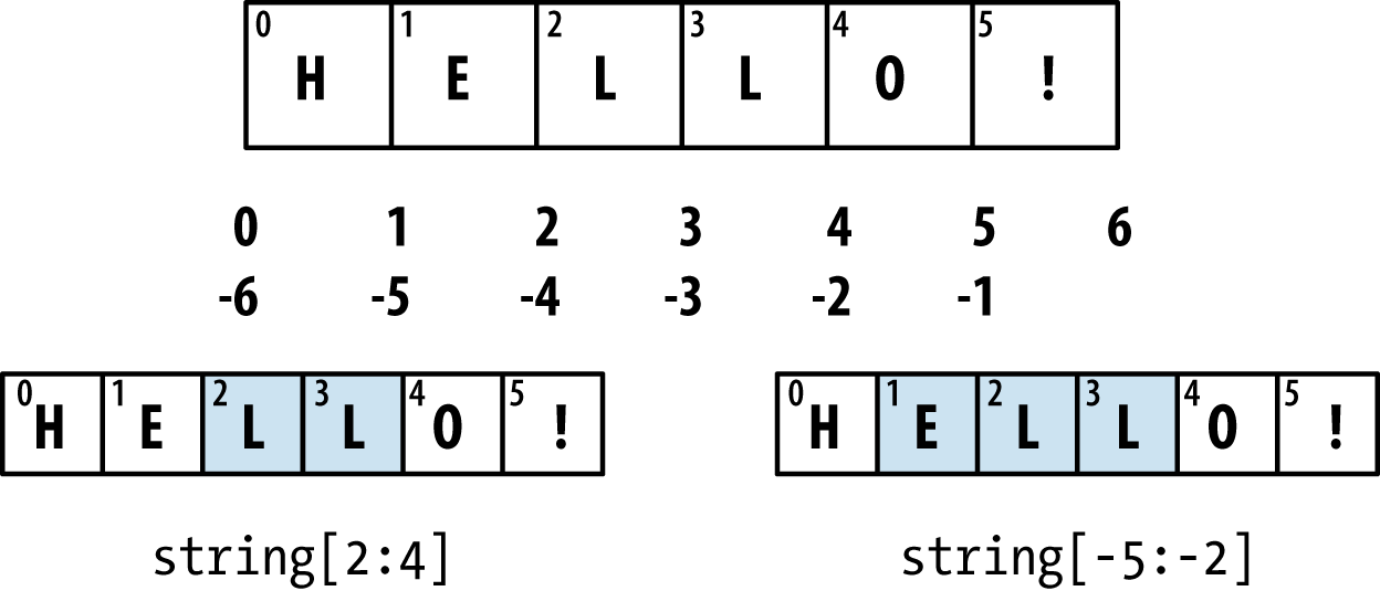
Figure 3-1. Illustration of Python slicing conventions
Built-in Sequence Functions
Python has a handful of useful sequence functions that you should familiarize yourself with and use at any opportunity.
enumerate
It’s common when iterating over a sequence to want to keep track of the index of the current item. A do-it-yourself approach would look like:
i=0forvalueincollection:# do something with valuei+=1
Since this is so common, Python has a built-in function, enumerate, which returns a sequence of
(i, value) tuples:
fori,valueinenumerate(collection):# do something with value
When you are indexing data, a helpful pattern that uses enumerate is computing a dict mapping the values of a sequence (which
are assumed to be unique) to their locations in the sequence:
In[83]:some_list=['foo','bar','baz']In[84]:mapping={}In[85]:fori,vinenumerate(some_list):....:mapping[v]=iIn[86]:mappingOut[86]:{'bar':1,'baz':2,'foo':0}
sorted
The sorted function returns
a new sorted list from the elements of any
sequence:
In[87]:sorted([7,1,2,6,0,3,2])Out[87]:[0,1,2,2,3,6,7]In[88]:sorted('horse race')Out[88]:[' ','a','c','e','e','h','o','r','r','s']
The sorted function accepts the same
arguments as the sort method on lists.
zip
zip “pairs” up the elements
of a number of lists, tuples, or other sequences to
create a list of tuples:
In[89]:seq1=['foo','bar','baz']In[90]:seq2=['one','two','three']In[91]:zipped=zip(seq1,seq2)In[92]:list(zipped)Out[92]:[('foo','one'),('bar','two'),('baz','three')]
zip can take an arbitrary
number of sequences, and the number of elements it produces is
determined by the shortest sequence:
In[93]:seq3=[False,True]In[94]:list(zip(seq1,seq2,seq3))Out[94]:[('foo','one',False),('bar','two',True)]
A very common use of zip is
simultaneously iterating over multiple sequences, possibly also
combined with enumerate:
In[95]:fori,(a,b)inenumerate(zip(seq1,seq2)):....:('{0}: {1}, {2}'.format(i,a,b))....:0:foo,one1:bar,two2:baz,three
Given a “zipped” sequence, zip can be applied in a clever way to
“unzip” the sequence. Another way to think about this is converting a
list of rows into a list of
columns. The syntax, which looks a bit magical,
is:
In[96]:pitchers=[('Nolan','Ryan'),('Roger','Clemens'),....:('Schilling','Curt')]In[97]:first_names,last_names=zip(*pitchers)In[98]:first_namesOut[98]:('Nolan','Roger','Schilling')In[99]:last_namesOut[99]:('Ryan','Clemens','Curt')
reversed
reversed iterates over
the elements of a sequence in reverse order:
In[100]:list(reversed(range(10)))Out[100]:[9,8,7,6,5,4,3,2,1,0]
Keep in mind that reversed is a generator (to
be discussed in some more detail later), so it does not create the
reversed sequence until materialized (e.g., with list or a for
loop).
dict
dict is likely the most important built-in Python data structure. A more
common name for it is hash map or
associative array. It is a flexibly sized
collection of key-value pairs, where
key and value are Python objects. One approach for creating one is to use
curly braces {} and colons to
separate keys and values:
In[101]:empty_dict={}In[102]:d1={'a':'some value','b':[1,2,3,4]}In[103]:d1Out[103]:{'a':'some value','b':[1,2,3,4]}
You can access, insert, or set elements using the same syntax as for accessing elements of a list or tuple:
In[104]:d1[7]='an integer'In[105]:d1Out[105]:{7:'an integer','a':'some value','b':[1,2,3,4]}In[106]:d1['b']Out[106]:[1,2,3,4]
You can check if a dict contains a key using the same syntax used for checking whether a list or tuple contains a value:
In[107]:'b'ind1Out[107]:True
You can delete values either using the del keyword
or the pop method (which
simultaneously returns the value and deletes the key):
In[108]:d1[5]='some value'In[109]:d1Out[109]:{5:'some value',7:'an integer','a':'some value','b':[1,2,3,4]}In[110]:d1['dummy']='another value'In[111]:d1Out[111]:{5:'some value',7:'an integer','a':'some value','b':[1,2,3,4],'dummy':'another value'}In[112]:deld1[5]In[113]:d1Out[113]:{7:'an integer','a':'some value','b':[1,2,3,4],'dummy':'another value'}In[114]:ret=d1.pop('dummy')In[115]:retOut[115]:'another value'In[116]:d1Out[116]:{7:'an integer','a':'some value','b':[1,2,3,4]}
The keys and values method give you iterators of the dict’s keys and values,
respectively. While the key-value pairs are not in any particular order,
these functions output the keys and values in the same order:
In[117]:list(d1.keys())Out[117]:['a','b',7]In[118]:list(d1.values())Out[118]:['some value',[1,2,3,4],'an integer']
You can merge one dict into another using the update
method:
In[119]:d1.update({'b':'foo','c':12})In[120]:d1Out[120]:{7:'an integer','a':'some value','b':'foo','c':12}
The update method changes dicts in-place, so
any existing keys in the data passed to update will
have their old values discarded.
Creating dicts from sequences
It’s common to occasionally end up with two sequences that you want to pair up element-wise in a dict. As a first cut, you might write code like this:
mapping={}forkey,valueinzip(key_list,value_list):mapping[key]=value
Since a dict is essentially a collection of 2-tuples, the dict function
accepts a list of 2-tuples:
In[121]:mapping=dict(zip(range(5),reversed(range(5))))In[122]:mappingOut[122]:{0:4,1:3,2:2,3:1,4:0}
Later we’ll talk about dict comprehensions, another elegant way to construct dicts.
Default values
It’s very common to have logic like:
ifkeyinsome_dict:value=some_dict[key]else:value=default_value
Thus, the dict methods get
and pop can take a default value to be returned, so that the above
if-else block can be written simply
as:
value=some_dict.get(key,default_value)
get by default will return
None if the key is not present,
while pop will raise an exception.
With setting values, a common case is for the
values in a dict to be other collections, like lists. For example, you
could imagine categorizing a list of words by their first letters as a
dict of lists:
In[123]:words=['apple','bat','bar','atom','book']In[124]:by_letter={}In[125]:forwordinwords:.....:letter=word[0].....:ifletternotinby_letter:.....:by_letter[letter]=[word].....:else:.....:by_letter[letter].append(word).....:In[126]:by_letterOut[126]:{'a':['apple','atom'],'b':['bat','bar','book']}
The setdefault dict method
is for precisely this purpose. The preceding for loop can be rewritten as:
forwordinwords:letter=word[0]by_letter.setdefault(letter,[]).append(word)
The built-in collections
module has a useful class, defaultdict, which makes this even easier. To create one, you pass a type or function for generating the
default value for each slot in the dict:
fromcollectionsimportdefaultdictby_letter=defaultdict(list)forwordinwords:by_letter[word[0]].append(word)
Valid dict key types
While the values of a dict can be any Python object, the keys generally
have to be immutable objects like scalar types (int, float, string) or
tuples (all the objects in the tuple need to be immutable, too). The
technical term here is hashability. You can
check whether an object is hashable (can be used as a key in a dict)
with the hash
function:
In[127]:hash('string')Out[127]:-305472831944956388In[128]:hash((1,2,(2,3)))Out[128]:1097636502276347782In[129]:hash((1,2,[2,3]))# fails because lists are mutable---------------------------------------------------------------------------TypeErrorTraceback(mostrecentcalllast)<ipython-input-129-473c35a62c0b>in<module>()---->1hash((1,2,[2,3]))# fails because lists are mutableTypeError:unhashabletype:'list'
To use a list as a key, one option is to convert it to a tuple, which can be hashed as long as its elements also can:
In[130]:d={}In[131]:d[tuple([1,2,3])]=5In[132]:dOut[132]:{(1,2,3):5}
set
A set is an unordered collection of unique elements. You can think of
them like dicts, but keys only, no values. A set can be created in two
ways: via the set function or via a set literal with
curly braces:
In[133]:set([2,2,2,1,3,3])Out[133]:{1,2,3}In[134]:{2,2,2,1,3,3}Out[134]:{1,2,3}
Sets support mathematical set operations like union, intersection, difference, and symmetric difference. Consider these two example sets:
In[135]:a={1,2,3,4,5}In[136]:b={3,4,5,6,7,8}
The union of these two sets is the set of distinct elements
occurring in either set. This can be computed with either the union method or the | binary operator:
In[137]:a.union(b)Out[137]:{1,2,3,4,5,6,7,8}In[138]:a|bOut[138]:{1,2,3,4,5,6,7,8}
The intersection contains the elements occurring in both sets.
The & operator or the
intersection method can be used:
In[139]:a.intersection(b)Out[139]:{3,4,5}In[140]:a&bOut[140]:{3,4,5}
See Table 3-1 for a list of commonly used set methods.
All of the logical set operations have in-place counterparts, which enable you to replace the contents of the set on the left side of the operation with the result. For very large sets, this may be more efficient:
In[141]:c=a.copy()In[142]:c|=bIn[143]:cOut[143]:{1,2,3,4,5,6,7,8}In[144]:d=a.copy()In[145]:d&=bIn[146]:dOut[146]:{3,4,5}
Like dicts, set elements generally must be immutable. To have list-like elements, you must convert it to a tuple:
In[147]:my_data=[1,2,3,4]In[148]:my_set={tuple(my_data)}In[149]:my_setOut[149]:{(1,2,3,4)}
You can also check if a set is a subset of (is contained in) or a superset of (contains all elements of) another set:
In[150]:a_set={1,2,3,4,5}In[151]:{1,2,3}.issubset(a_set)Out[151]:TrueIn[152]:a_set.issuperset({1,2,3})Out[152]:True
Sets are equal if and only if their contents are equal:
In[153]:{1,2,3}=={3,2,1}Out[153]:True
List, Set, and Dict Comprehensions
List comprehensions are one of the most-loved Python language features. They allow you to concisely form a new list by filtering the elements of a collection, transforming the elements passing the filter in one concise expression. They take the basic form:
[exprfor val in collection ifcondition]
This is equivalent to the following for loop:
result = []
for val in collection:
    if condition:
        result.append(expr)
The filter condition can be omitted, leaving only the expression. For example, given a list of strings, we could filter out strings with length 2 or less and also convert them to uppercase like this:
In[154]:strings=['a','as','bat','car','dove','python']In[155]:[x.upper()forxinstringsiflen(x)>2]Out[155]:['BAT','CAR','DOVE','PYTHON']
Set and dict comprehensions are a natural extension, producing sets and dicts in an idiomatically similar way instead of lists. A dict comprehension looks like this:
dict_comp = {key-expr : value-expr for value in collection
             if condition}
A set comprehension looks like the equivalent list comprehension except with curly braces instead of square brackets:
set_comp = {expr for value in collection if condition}Like list comprehensions, set and dict comprehensions are mostly conveniences, but they similarly can make code both easier to write and read. Consider the list of strings from before. Suppose we wanted a set containing just the lengths of the strings contained in the collection; we could easily compute this using a set comprehension:
In[156]:unique_lengths={len(x)forxinstrings}In[157]:unique_lengthsOut[157]:{1,2,3,4,6}
We could also express this more functionally using the map function, introduced
shortly:
In[158]:set(map(len,strings))Out[158]:{1,2,3,4,6}
As a simple dict comprehension example, we could create a lookup map of these strings to their locations in the list:
In[159]:loc_mapping={val:indexforindex,valinenumerate(strings)}In[160]:loc_mappingOut[160]:{'a':0,'as':1,'bat':2,'car':3,'dove':4,'python':5}
Nested list comprehensions
Suppose we have a list of lists containing some English and Spanish names:
In[161]:all_data=[['John','Emily','Michael','Mary','Steven'],.....:['Maria','Juan','Javier','Natalia','Pilar']]
You might have gotten these names from a couple of files and
decided to organize them by language. Now, suppose we wanted to get a
single list containing all names with two or more e’s in them. We could certainly do this with
a simple for
loop:
names_of_interest=[]fornamesinall_data:enough_es=[namefornameinnamesifname.count('e')>=2]names_of_interest.extend(enough_es)
You can actually wrap this whole operation up in a single nested list comprehension, which will look like:
In[162]:result=[namefornamesinall_datafornameinnames.....:ifname.count('e')>=2]In[163]:resultOut[163]:['Steven']
At first, nested list comprehensions are a bit hard to wrap your
head around. The for parts of the
list comprehension are arranged according to the order of nesting, and
any filter condition is put at the end as before. Here is another
example where we “flatten” a list of tuples of integers into a simple
list of integers:
In[164]:some_tuples=[(1,2,3),(4,5,6),(7,8,9)]In[165]:flattened=[xfortupinsome_tuplesforxintup]In[166]:flattenedOut[166]:[1,2,3,4,5,6,7,8,9]
Keep in mind that the order of the for expressions would be the same if you
wrote a nested for loop instead of
a list comprehension:
flattened=[]fortupinsome_tuples:forxintup:flattened.append(x)
You can have arbitrarily many levels of nesting, though if you have more than two or three levels of nesting you should probably start to question whether this makes sense from a code readability standpoint. It’s important to distinguish the syntax just shown from a list comprehension inside a list comprehension, which is also perfectly valid:
In[167]:[[xforxintup]fortupinsome_tuples]Out[167]:[[1,2,3],[4,5,6],[7,8,9]]
This produces a list of lists, rather than a flattened list of all of the inner elements.
3.2 Functions
Functions are the primary and most important method of code organization and reuse in Python. As a rule of thumb, if you anticipate needing to repeat the same or very similar code more than once, it may be worth writing a reusable function. Functions can also help make your code more readable by giving a name to a group of Python statements.
Functions are declared with the def keyword and
returned from with the return
keyword:
defmy_function(x,y,z=1.5):ifz>1:returnz*(x+y)else:returnz/(x+y)
There is no issue with having multiple return statements. If Python reaches the end of a function without encountering a return
statement, None is returned
automatically.
Each function can have positional arguments and
keyword arguments. Keyword arguments are most
commonly used to specify default values or optional arguments. In the
preceding function, x and y are positional arguments while z is a keyword argument. This means that the
function can be called in any of these ways:
my_function(5,6,z=0.7)my_function(3.14,7,3.5)my_function(10,20)
The main restriction on function arguments is that the keyword arguments must follow the positional arguments (if any). You can specify keyword arguments in any order; this frees you from having to remember which order the function arguments were specified in and only what their names are.
Note
It is possible to use keywords for passing positional arguments as well. In the preceding example, we could also have written:
my_function(x=5,y=6,z=7)my_function(y=6,x=5,z=7)
In some cases this can help with readability.
Namespaces, Scope, and Local Functions
Functions can access variables in two different scopes: global and local. An alternative and more descriptive name describing a variable scope in Python is a namespace. Any variables that are assigned within a function by default are assigned to the local namespace. The local namespace is created when the function is called and immediately populated by the function’s arguments. After the function is finished, the local namespace is destroyed (with some exceptions that are outside the purview of this chapter). Consider the following function:
deffunc():a=[]foriinrange(5):a.append(i)
When func() is called, the empty
list a is created, five elements are
appended, and then a is destroyed when
the function exits. Suppose instead we had declared a as follows:
a=[]deffunc():foriinrange(5):a.append(i)
Assigning variables outside of the function’s scope is possible,
but those variables must be declared as global via the global
keyword:
In[168]:a=NoneIn[169]:defbind_a_variable():.....:globala.....:a=[].....:bind_a_variable().....:In[170]:(a)[]
Caution
I generally discourage use of the global keyword. Typically global variables
are used to store some kind of state in a system. If you find yourself
using a lot of them, it may indicate a need for object-oriented
programming (using classes).
Returning Multiple Values
When I first programmed in Python after having programmed in Java and C++, one of my favorite features was the ability to return multiple values from a function with simple syntax. Here’s an example:
deff():a=5b=6c=7returna,b,ca,b,c=f()
In data analysis and other scientific applications, you may find yourself doing this often. What’s happening here is that the function is actually just returning one object, namely a tuple, which is then being unpacked into the result variables. In the preceding example, we could have done this instead:
return_value=f()
In this case, return_value
would be a 3-tuple with the three returned variables. A potentially
attractive alternative to returning multiple values like before might be
to return a dict instead:
deff():a=5b=6c=7return{'a':a,'b':b,'c':c}
This alternative technique can be useful depending on what you are trying to do.
Functions Are Objects
Since Python functions are objects, many constructs can be easily expressed that are difficult to do in other languages. Suppose we were doing some data cleaning and needed to apply a bunch of transformations to the following list of strings:
In[171]:states=[' Alabama ','Georgia!','Georgia','georgia','FlOrIda',.....:'south carolina##','West virginia?']
Anyone who has ever worked with user-submitted survey data has
seen messy results like these. Lots of things need to happen to make
this list of strings uniform and ready for analysis: stripping whitespace, removing punctuation symbols, and standardizing on proper
capitalization. One way to do this is to use built-in string methods
along with the re standard library module for regular expressions:
importredefclean_strings(strings):result=[]forvalueinstrings:value=value.strip()value=re.sub('[!#?]','',value)value=value.title()result.append(value)returnresult
The result looks like this:
In[173]:clean_strings(states)Out[173]:['Alabama','Georgia','Georgia','Georgia','Florida','South Carolina','West Virginia']
An alternative approach that you may find useful is to make a list of the operations you want to apply to a particular set of strings:
defremove_punctuation(value):returnre.sub('[!#?]','',value)clean_ops=[str.strip,remove_punctuation,str.title]defclean_strings(strings,ops):result=[]forvalueinstrings:forfunctioninops:value=function(value)result.append(value)returnresult
Then we have the following:
In[175]:clean_strings(states,clean_ops)Out[175]:['Alabama','Georgia','Georgia','Georgia','Florida','South Carolina','West Virginia']
A more functional pattern like this enables
you to easily modify how the strings are transformed at a very high
level. The clean_strings function is
also now more reusable and generic.
You can use functions as arguments to other functions like the
built-in map function,
which applies a function to a sequence of some kind:
In[176]:forxinmap(remove_punctuation,states):.....:(x)AlabamaGeorgiaGeorgiageorgiaFlOrIdasouthcarolinaWestvirginia
Anonymous (Lambda) Functions
Python has support for so-called anonymous or
lambda functions, which are a way of writing
functions consisting of a single statement, the result of which is the
return value. They are defined with the lambda keyword, which has no meaning other
than “we are declaring an anonymous function”:
defshort_function(x):returnx*2equiv_anon=lambdax:x*2
I usually refer to these as lambda functions in the rest of the book. They are especially convenient in data analysis because, as you’ll see, there are many cases where data transformation functions will take functions as arguments. It’s often less typing (and clearer) to pass a lambda function as opposed to writing a full-out function declaration or even assigning the lambda function to a local variable. For example, consider this silly example:
defapply_to_list(some_list,f):return[f(x)forxinsome_list]ints=[4,0,1,5,6]apply_to_list(ints,lambdax:x*2)
You could also have written [x * 2 for x
in ints], but here we were able to succinctly pass a custom
operator to the apply_to_list
function.
As another example, suppose you wanted to sort a collection of strings by the number of distinct letters in each string:
In[177]:strings=['foo','card','bar','aaaa','abab']
Here we could pass a lambda function to the list’s sort
method:
In[178]:strings.sort(key=lambdax:len(set(list(x))))In[179]:stringsOut[179]:['aaaa','foo','abab','bar','card']
Currying: Partial Argument Application
Currying is computer science jargon (named after the mathematician Haskell Curry) that means deriving new functions from existing ones by partial argument application. For example, suppose we had a trivial function that adds two numbers together:
defadd_numbers(x,y):returnx+y
Using this function, we could derive a new function of one
variable, add_five, that adds 5 to
its argument:
add_five=lambday:add_numbers(5,y)
The second argument to add_numbers is said to be
curried. There’s nothing very fancy here, as all
we’ve really done is define a new function that calls an existing
function. The built-in functools
module can simplify this process using the partial
function:
fromfunctoolsimportpartialadd_five=partial(add_numbers,5)
Generators
Having a consistent way to iterate over sequences, like objects in a list or lines in a file, is an important Python feature. This is accomplished by means of the iterator protocol, a generic way to make objects iterable. For example, iterating over a dict yields the dict keys:
In[180]:some_dict={'a':1,'b':2,'c':3}In[181]:forkeyinsome_dict:.....:(key)abc
When you write for key in
some_dict, the Python interpreter first attempts to create an
iterator out of some_dict:
In[182]:dict_iterator=iter(some_dict)In[183]:dict_iteratorOut[183]:<dict_keyiteratorat0x7ff84e90ee58>
An iterator is any object that will yield objects to the Python
interpreter when used in a context like a for loop.
Most methods expecting a list or list-like object will also accept any
iterable object. This includes built-in methods such as min, max,
and sum, and type constructors like
list and tuple:
In[184]:list(dict_iterator)Out[184]:['a','b','c']
A generator is a concise way to construct a
new iterable object. Whereas normal functions execute and return a
single result at a time, generators return a sequence of multiple
results lazily, pausing after each one until the next one is requested.
To create a generator, use the yield keyword
instead of return in a
function:
defsquares(n=10):('Generating squares from 1 to {0}'.format(n**2))foriinrange(1,n+1):yieldi**2
When you actually call the generator, no code is immediately executed:
In[186]:gen=squares()In[187]:genOut[187]:<generatorobjectsquaresat0x7ff84e92bbf8>
It is not until you request elements from the generator that it begins executing its code:
In[188]:forxingen:.....:(x,end=' ')Generatingsquaresfrom1to100149162536496481100
Generator expresssions
Another even more concise way to make a generator is by using a generator expression. This is a generator analogue to list, dict, and set comprehensions; to create one, enclose what would otherwise be a list comprehension within parentheses instead of brackets:
In[189]:gen=(x**2forxinrange(100))In[190]:genOut[190]:<generatorobject<genexpr>at0x7ff84e92b150>
This is completely equivalent to the following more verbose generator:
def_make_gen():forxinrange(100):yieldx**2gen=_make_gen()
Generator expressions can be used instead of list comprehensions as function arguments in many cases:
In[191]:sum(x**2forxinrange(100))Out[191]:328350In[192]:dict((i,i**2)foriinrange(5))Out[192]:{0:0,1:1,2:4,3:9,4:16}
itertools module
The standard library itertools module has a collection of generators for many common data
algorithms. For example, groupby
takes any sequence and a function, grouping consecutive elements in
the sequence by return value of the function. Here’s an
example:
In[193]:importitertoolsIn[194]:first_letter=lambdax:x[0]In[195]:names=['Alan','Adam','Wes','Will','Albert','Steven']In[196]:forletter,namesinitertools.groupby(names,first_letter):.....:(letter,list(names))# names is a generatorA['Alan','Adam']W['Wes','Will']A['Albert']S['Steven']
See Table 3-2 for a list of a few other
itertools functions I’ve frequently found helpful. You may like to
check out the official
Python documentation for more on this useful built-in utility
module.
Errors and Exception Handling
Handling Python errors or exceptions gracefully is an
important part of building robust programs. In data analysis
applications, many functions only work on certain kinds of input. As an
example, Python’s float function is
capable of casting a string to a floating-point number, but fails with ValueError
on improper inputs:
In[197]:float('1.2345')Out[197]:1.2345In[198]:float('something')---------------------------------------------------------------------------ValueErrorTraceback(mostrecentcalllast)<ipython-input-198-2649e4ade0e6>in<module>()---->1float('something')ValueError:couldnotconvertstringtofloat:'something'
Suppose we wanted a version of float that fails gracefully, returning the
input argument. We can do this by writing a function that encloses the
call to float in a try/except block:
defattempt_float(x):try:returnfloat(x)except:returnx
The code in the except part of
the block will only be executed if float(x) raises an exception:
In[200]:attempt_float('1.2345')Out[200]:1.2345In[201]:attempt_float('something')Out[201]:'something'
You might notice that float can
raise exceptions other than ValueError:
In[202]:float((1,2))---------------------------------------------------------------------------TypeErrorTraceback(mostrecentcalllast)<ipython-input-202-82f777b0e564>in<module>()---->1float((1,2))TypeError:float()argumentmustbeastringoranumber,not'tuple'
You might want to only suppress ValueError, since a TypeError (the input was not a string or numeric value) might indicate a
legitimate bug in your program. To do that, write the exception type
after except:
defattempt_float(x):try:returnfloat(x)exceptValueError:returnx
We have then:
In[204]:attempt_float((1,2))---------------------------------------------------------------------------TypeErrorTraceback(mostrecentcalllast)<ipython-input-204-8b0026e9e6b7>in<module>()---->1attempt_float((1,2))<ipython-input-203-d99a2a135508>inattempt_float(x)1defattempt_float(x):2try:---->3returnfloat(x)4exceptValueError:5returnxTypeError:float()argumentmustbeastringoranumber,not'tuple'
You can catch multiple exception types by writing a tuple of exception types instead (the parentheses are required):
defattempt_float(x):try:returnfloat(x)except(TypeError,ValueError):returnx
In some cases, you may not want to suppress an exception, but you
want some code to be executed regardless of whether the code in the
try block succeeds or not. To do
this, use finally:
f=open(path,'w')try:write_to_file(f)finally:f.close()
Here, the file handle f will
always get closed. Similarly, you can have code
that executes only if the try: block
succeeds using else:
f=open(path,'w')try:write_to_file(f)except:('Failed')else:('Succeeded')finally:f.close()
Exceptions in IPython
If an exception is raised while you are %run-ing a
script or executing any statement, IPython will by
default print a full call stack trace (traceback) with a few lines of
context around the position at each point in the stack:
In[10]:%runexamples/ipython_bug.py---------------------------------------------------------------------------AssertionErrorTraceback(mostrecentcalllast)/home/wesm/code/pydata-book/examples/ipython_bug.pyin<module>()13throws_an_exception()14--->15calling_things()/home/wesm/code/pydata-book/examples/ipython_bug.pyincalling_things()11defcalling_things():12works_fine()--->13throws_an_exception()1415calling_things()/home/wesm/code/pydata-book/examples/ipython_bug.pyinthrows_an_exception()7a=58b=6---->9assert(a+b==10)1011defcalling_things():AssertionError:
Having additional context by itself is a big advantage over the
standard Python interpreter (which does not provide any additional
context). You can control the amount of context shown using the %xmode
magic command, from Plain (same as the standard
Python interpreter) to Verbose (which inlines
function argument values and more). As you will see later in the
chapter, you can step into the stack (using the
%debug or %pdb magics) after an error has occurred for interactive post-mortem debugging.
3.3 Files and the Operating System
Most of this book uses high-level tools like pandas.read_csv to read data files from disk into Python data structures.
However, it’s important to understand the basics of how to work with files
in Python. Fortunately, it’s very simple, which is one reason why Python
is so popular for text and file munging.
To open a file for reading or writing, use the built-in open function
with either a relative or absolute file path:
In[207]:path='examples/segismundo.txt'In[208]:f=open(path)
By default, the file is opened in read-only mode 'r'. We can then treat the file handle f like a list and iterate over the lines like
so:
forlineinf:pass
The lines come out of the file with the end-of-line (EOL) markers intact, so you’ll often see code to get an EOL-free list of lines in a file like:
In[209]:lines=[x.rstrip()forxinopen(path)]In[210]:linesOut[210]:['Sueña el rico en su riqueza,','que más cuidados le ofrece;','','sueña el pobre que padece','su miseria y su pobreza;','','sueña el que a medrar empieza,','sueña el que afana y pretende,','sueña el que agravia y ofende,','','y en el mundo, en conclusión,','todos sueñan lo que son,','aunque ninguno lo entiende.','']
When you use open to create file objects, it is
important to explicitly close the file when you are finished with it.
Closing the file releases its resources back to the operating system:
In[211]:f.close()
One of the ways to make it easier to clean up open files is to use
the with statement:
In[212]:withopen(path)asf:.....:lines=[x.rstrip()forxinf]
This will automatically close the file f when
exiting the with block.
If we had typed f = open(path,
'w'), a new file at
examples/segismundo.txt would have been created (be
careful!), overwriting any one in its place. There is also the
'x' file mode, which creates a writable file but fails
if the file path already exists. See Table 3-3
for a list of all valid file read/write modes.
For readable files, some of the most commonly used methods are read,
seek, and tell.
read returns a certain number of characters from the
file. What constitutes a “character” is determined by the file’s encoding
(e.g., UTF-8) or simply raw bytes if the file is opened in binary
mode:
In[213]:f=open(path)In[214]:f.read(10)Out[214]:'Sueña el r'In[215]:f2=open(path,'rb')# Binary modeIn[216]:f2.read(10)Out[216]:b'Sue\xc3\xb1a el '
The read method advances the file handle’s
position by the number of bytes read. tell gives you the current
position:
In[217]:f.tell()Out[217]:11In[218]:f2.tell()Out[218]:10
Even though we read 10 characters from the file, the position is 11
because it took that many bytes to decode 10 characters using the default
encoding. You can check the default encoding in the sys module:
In[219]:importsysIn[220]:sys.getdefaultencoding()Out[220]:'utf-8'
seek changes the file position to the indicated
byte in the file:
In[221]:f.seek(3)Out[221]:3In[222]:f.read(1)Out[222]:'ñ'
Lastly, we remember to close the files:
In[223]:f.close()In[224]:f2.close()
To write text to a file, you can use the
file’s write or writelines methods. For example, we could create
a version of prof_mod.py with no blank lines like
so:
In[225]:withopen('tmp.txt','w')ashandle:.....:handle.writelines(xforxinopen(path)iflen(x)>1)In[226]:withopen('tmp.txt')asf:.....:lines=f.readlines()In[227]:linesOut[227]:['Sueña el rico en su riqueza,\n','que más cuidados le ofrece;\n','sueña el pobre que padece\n','su miseria y su pobreza;\n','sueña el que a medrar empieza,\n','sueña el que afana y pretende,\n','sueña el que agravia y ofende,\n','y en el mundo, en conclusión,\n','todos sueñan lo que son,\n','aunque ninguno lo entiende.\n']
See Table 3-4 for many of the most commonly used file methods.
Bytes and Unicode with Files
The default behavior for Python files (whether readable or writable) is
text mode, which means that you intend to work with
Python strings (i.e., Unicode). This contrasts with binary mode, which you can
obtain by appending b onto the file mode. Let’s look
at the file (which contains non-ASCII characters with UTF-8 encoding)
from the previous section:
In[230]:withopen(path)asf:.....:chars=f.read(10)In[231]:charsOut[231]:'Sueña el r'
UTF-8 is a variable-length Unicode encoding, so when I requested some
number of characters from the file, Python reads enough bytes (which
could be as few as 10 or as many as 40 bytes) from the file to decode
that many characters. If I open the file in 'rb' mode
instead, read requests exact numbers of bytes:
In[232]:withopen(path,'rb')asf:.....:data=f.read(10)In[233]:dataOut[233]:b'Sue\xc3\xb1a el '
Depending on the text encoding, you may be able to decode the
bytes to a str object yourself, but only if each of
the encoded Unicode characters is fully formed:
In[234]:data.decode('utf8')Out[234]:'Sueña el 'In[235]:data[:4].decode('utf8')---------------------------------------------------------------------------UnicodeDecodeErrorTraceback(mostrecentcalllast)<ipython-input-235-0ad9ad6a11bd>in<module>()---->1data[:4].decode('utf8')UnicodeDecodeError:'utf-8'codeccan't decode byte 0xc3 in position 3: unexpectedendofdata
Text mode, combined with the encoding option of
open, provides a convenient way to convert from one Unicode encoding to
another:
In[236]:sink_path='sink.txt'In[237]:withopen(path)assource:.....:withopen(sink_path,'xt',encoding='iso-8859-1')assink:.....:sink.write(source.read())In[238]:withopen(sink_path,encoding='iso-8859-1')asf:.....:(f.read(10))Sueñaelr
Beware using seek when opening files in any mode other than binary. If the file
position falls in the middle of the bytes defining a Unicode character,
then subsequent reads will result in an error:
In[240]:f=open(path)In[241]:f.read(5)Out[241]:'Sueña'In[242]:f.seek(4)Out[242]:4In[243]:f.read(1)---------------------------------------------------------------------------UnicodeDecodeErrorTraceback(mostrecentcalllast)<ipython-input-243-5a354f952aa4>in<module>()---->1f.read(1)/miniconda/envs/book-env/lib/python3.6/codecs.pyindecode(self,input,final)319# decode input (taking the buffer into account)320data=self.buffer+input-->321(result,consumed)=self._buffer_decode(data,self.errors,final)322# keep undecoded input until the next call323self.buffer=data[consumed:]UnicodeDecodeError:'utf-8'codeccan't decode byte 0xb1 in position 0: invalid startbyteIn[244]:f.close()
If you find yourself regularly doing data analysis on non-ASCII text data, mastering Python’s Unicode functionality will prove valuable. See Python’s online documentation for much more.
3.4 Conclusion
With some of the basics and the Python environment and language now under our belt, it’s time to move on and learn about NumPy and array-oriented computing in Python.