Second Edition
Data Wrangling with Pandas, NumPy, and IPython
Copyright © 2018 William McKinney. All rights reserved.
Printed in the United States of America.
Published by O’Reilly Media, Inc., 1005 Gravenstein Highway North, Sebastopol, CA 95472.
O’Reilly books may be purchased for educational, business, or sales promotional use. Online editions are also available for most titles (http://oreilly.com/safari). For more information, contact our corporate/institutional sales department: 800-998-9938 or corporate@oreilly.com.
See http://oreilly.com/catalog/errata.csp?isbn=9781491957660 for release details.
The O’Reilly logo is a registered trademark of O’Reilly Media, Inc. Python for Data Analysis, the cover image, and related trade dress are trademarks of O’Reilly Media, Inc.
While the publisher and the author have used good faith efforts to ensure that the information and instructions contained in this work are accurate, the publisher and the author disclaim all responsibility for errors or omissions, including without limitation responsibility for damages resulting from the use of or reliance on this work. Use of the information and instructions contained in this work is at your own risk. If any code samples or other technology this work contains or describes is subject to open source licenses or the intellectual property rights of others, it is your responsibility to ensure that your use thereof complies with such licenses and/or rights.
978-1-491-95766-0
[M]
The first edition of this book was published in 2012, during a time when open source data analysis libraries for Python (such as pandas) were very new and developing rapidly. In this updated and expanded second edition, I have overhauled the chapters to account both for incompatible changes and deprecations as well as new features that have occurred in the last five years. I’ve also added fresh content to introduce tools that either did not exist in 2012 or had not matured enough to make the first cut. Finally, I have tried to avoid writing about new or cutting-edge open source projects that may not have had a chance to mature. I would like readers of this edition to find that the content is still almost as relevant in 2020 or 2021 as it is in 2017.
The major updates in this second edition include:
All code, including the Python tutorial, updated for Python 3.6 (the first edition used Python 2.7)
Updated Python installation instructions for the Anaconda Python Distribution and other needed Python packages
Updates for the latest versions of the pandas library in 2017
A new chapter on some more advanced pandas tools, and some other usage tips
A brief introduction to using statsmodels and scikit-learn
I also reorganized a significant portion of the content from the first edition to make the book more accessible to newcomers.
The following typographical conventions are used in this book:
Indicates new terms, URLs, email addresses, filenames, and file extensions.
Constant widthUsed for program listings, as well as within paragraphs to refer to program elements such as variable or function names, databases, data types, environment variables, statements, and keywords.
Constant width boldShows commands or other text that should be typed literally by the user.
Constant width italicShows text that should be replaced with user-supplied values or by values determined by context.
This element signifies a tip or suggestion.
This element signifies a general note.
This element indicates a warning or caution.
You can find data files and related material for each chapter is available in this book’s GitHub repository at http://github.com/wesm/pydata-book.
This book is here to help you get your job done. In general, if example code is offered with this book, you may use it in your programs and documentation. You do not need to contact us for permission unless you’re reproducing a significant portion of the code. For example, writing a program that uses several chunks of code from this book does not require permission. Selling or distributing a CD-ROM of examples from O’Reilly books does require permission. Answering a question by citing this book and quoting example code does not require permission. Incorporating a significant amount of example code from this book into your product’s documentation does require permission.
We appreciate, but do not require, attribution. An attribution usually includes the title, author, publisher, and ISBN. For example: “Python for Data Analysis by Wes McKinney (O’Reilly). Copyright 2017 Wes McKinney, 978-1-491-95766-0.”
If you feel your use of code examples falls outside fair use or the permission given above, feel free to contact us at permissions@oreilly.com.
Safari (formerly Safari Books Online) is a membership-based training and reference platform for enterprise, government, educators, and individuals.
Members have access to thousands of books, training videos, Learning Paths, interactive tutorials, and curated playlists from over 250 publishers, including O’Reilly Media, Harvard Business Review, Prentice Hall Professional, Addison-Wesley Professional, Microsoft Press, Sams, Que, Peachpit Press, Adobe, Focal Press, Cisco Press, John Wiley & Sons, Syngress, Morgan Kaufmann, IBM Redbooks, Packt, Adobe Press, FT Press, Apress, Manning, New Riders, McGraw-Hill, Jones & Bartlett, and Course Technology, among others.
For more information, please visit http://oreilly.com/safari.
Please address comments and questions concerning this book to the publisher:
We have a web page for this book, where we list errata, examples, and any additional information. You can access this page at http://bit.ly/python_data_analysis_2e.
To comment or ask technical questions about this book, send email to bookquestions@oreilly.com.
For more information about our books, courses, conferences, and news, see our website at http://www.oreilly.com.
Find us on Facebook: http://facebook.com/oreilly
Follow us on Twitter: http://twitter.com/oreillymedia
Watch us on YouTube: http://www.youtube.com/oreillymedia
This work is the product of many years of fruitful discussions, collaborations, and assistance with and from many people around the world. I’d like to thank a few of them.
Our dear friend and colleague John D. Hunter passed away after a battle with colon cancer on August 28, 2012. This was only a short time after I’d completed the final manuscript for this book’s first edition.
John’s impact and legacy in the Python scientific and data communities would be hard to overstate. In addition to developing matplotlib in the early 2000s (a time when Python was not nearly so popular), he helped shape the culture of a critical generation of open source developers who’ve become pillars of the Python ecosystem that we now often take for granted.
I was lucky enough to connect with John early in my open source career in January 2010, just after releasing pandas 0.1. His inspiration and mentorship helped me push forward, even in the darkest of times, with my vision for pandas and Python as a first-class data analysis language.
John was very close with Fernando Pérez and Brian Granger, pioneers of IPython, Jupyter, and many other initiatives in the Python community. We had hoped to work on a book together, the four of us, but I ended up being the one with the most free time. I am sure he would be proud of what we’ve accomplished, as individuals and as a community, over the last five years.
It has been five years almost to the day since I completed the manuscript for this book’s first edition in July 2012. A lot has changed. The Python community has grown immensely, and the ecosystem of open source software around it has flourished.
This new edition of the book would not exist if not for the tireless efforts of the pandas core developers, who have grown the project and its user community into one of the cornerstones of the Python data science ecosystem. These include, but are not limited to, Tom Augspurger, Joris van den Bossche, Chris Bartak, Phillip Cloud, gfyoung, Andy Hayden, Masaaki Horikoshi, Stephan Hoyer, Adam Klein, Wouter Overmeire, Jeff Reback, Chang She, Skipper Seabold, Jeff Tratner, and y-p.
On the actual writing of this second edition, I would like to thank the O’Reilly staff who helped me patiently with the writing process. This includes Marie Beaugureau, Ben Lorica, and Colleen Toporek. I again had outstanding technical reviewers with Tom Augpurger, Paul Barry, Hugh Brown, Jonathan Coe, and Andreas Müller contributing. Thank you.
This book’s first edition has been translated into many foreign languages, including Chinese, French, German, Japanese, Korean, and Russian. Translating all this content and making it available to a broader audience is a huge and often thankless effort. Thank you for helping more people in the world learn how to program and use data analysis tools.
I am also lucky to have had support for my continued open source development efforts from Cloudera and Two Sigma Investments over the last few years. With open source software projects more thinly resourced than ever relative to the size of user bases, it is becoming increasingly important for businesses to provide support for development of key open source projects. It’s the right thing to do.
It would have been difficult for me to write this book without the support of a large number of people.
On the O’Reilly staff, I’m very grateful for my editors, Meghan Blanchette and Julie Steele, who guided me through the process. Mike Loukides also worked with me in the proposal stages and helped make the book a reality.
I received a wealth of technical review from a large cast of characters. In particular, Martin Blais and Hugh Brown were incredibly helpful in improving the book’s examples, clarity, and organization from cover to cover. James Long, Drew Conway, Fernando Pérez, Brian Granger, Thomas Kluyver, Adam Klein, Josh Klein, Chang She, and Stéfan van der Walt each reviewed one or more chapters, providing pointed feedback from many different perspectives.
I got many great ideas for examples and datasets from friends and colleagues in the data community, among them: Mike Dewar, Jeff Hammerbacher, James Johndrow, Kristian Lum, Adam Klein, Hilary Mason, Chang She, and Ashley Williams.
I am of course indebted to the many leaders in the open source scientific Python community who’ve built the foundation for my development work and gave encouragement while I was writing this book: the IPython core team (Fernando Pérez, Brian Granger, Min Ragan-Kelly, Thomas Kluyver, and others), John Hunter, Skipper Seabold, Travis Oliphant, Peter Wang, Eric Jones, Robert Kern, Josef Perktold, Francesc Alted, Chris Fonnesbeck, and too many others to mention. Several other people provided a great deal of support, ideas, and encouragement along the way: Drew Conway, Sean Taylor, Giuseppe Paleologo, Jared Lander, David Epstein, John Krowas, Joshua Bloom, Den Pilsworth, John Myles-White, and many others I’ve forgotten.
I’d also like to thank a number of people from my formative years. First, my former AQR colleagues who’ve cheered me on in my pandas work over the years: Alex Reyfman, Michael Wong, Tim Sargen, Oktay Kurbanov, Matthew Tschantz, Roni Israelov, Michael Katz, Chris Uga, Prasad Ramanan, Ted Square, and Hoon Kim. Lastly, my academic advisors Haynes Miller (MIT) and Mike West (Duke).
I received significant help from Phillip Cloud and Joris Van den Bossche in 2014 to update the book’s code examples and fix some other inaccuracies due to changes in pandas.
On the personal side, Casey provided invaluable day-to-day support during the writing process, tolerating my highs and lows as I hacked together the final draft on top of an already overcommitted schedule. Lastly, my parents, Bill and Kim, taught me to always follow my dreams and to never settle for less.
This book is concerned with the nuts and bolts of manipulating, processing, cleaning, and crunching data in Python. My goal is to offer a guide to the parts of the Python programming language and its data-oriented library ecosystem and tools that will equip you to become an effective data analyst. While “data analysis” is in the title of the book, the focus is specifically on Python programming, libraries, and tools as opposed to data analysis methodology. This is the Python programming you need for data analysis.
When I say “data,” what am I referring to exactly? The primary focus is on structured data, a deliberately vague term that encompasses many different common forms of data, such as:
Tabular or spreadsheet-like data in which each column may be a different type (string, numeric, date, or otherwise). This includes most kinds of data commonly stored in relational databases or tab- or comma-delimited text files.
Multidimensional arrays (matrices).
Multiple tables of data interrelated by key columns (what would be primary or foreign keys for a SQL user).
Evenly or unevenly spaced time series.
This is by no means a complete list. Even though it may not always be obvious, a large percentage of datasets can be transformed into a structured form that is more suitable for analysis and modeling. If not, it may be possible to extract features from a dataset into a structured form. As an example, a collection of news articles could be processed into a word frequency table, which could then be used to perform sentiment analysis.
Most users of spreadsheet programs like Microsoft Excel, perhaps the most widely used data analysis tool in the world, will not be strangers to these kinds of data.
For many people, the Python programming language has strong appeal. Since its first appearance in 1991, Python has become one of the most popular interpreted programming languages, along with Perl, Ruby, and others. Python and Ruby have become especially popular since 2005 or so for building websites using their numerous web frameworks, like Rails (Ruby) and Django (Python). Such languages are often called scripting languages, as they can be used to quickly write small programs, or scripts to automate other tasks. I don’t like the term “scripting language,” as it carries a connotation that they cannot be used for building serious software. Among interpreted languages, for various historical and cultural reasons, Python has developed a large and active scientific computing and data analysis community. In the last 10 years, Python has gone from a bleeding-edge or “at your own risk” scientific computing language to one of the most important languages for data science, machine learning, and general software development in academia and industry.
For data analysis and interactive computing and data visualization, Python will inevitably draw comparisons with other open source and commercial programming languages and tools in wide use, such as R, MATLAB, SAS, Stata, and others. In recent years, Python’s improved support for libraries (such as pandas and scikit-learn) has made it a popular choice for data analysis tasks. Combined with Python’s overall strength for general-purpose software engineering, it is an excellent option as a primary language for building data applications.
Part of Python’s success in scientific computing is the ease of integrating C, C++, and FORTRAN code. Most modern computing environments share a similar set of legacy FORTRAN and C libraries for doing linear algebra, optimization, integration, fast Fourier transforms, and other such algorithms. The same story has held true for many companies and national labs that have used Python to glue together decades’ worth of legacy software.
Many programs consist of small portions of code where most of the time is spent, with large amounts of “glue code” that doesn’t run often. In many cases, the execution time of the glue code is insignificant; effort is most fruitfully invested in optimizing the computational bottlenecks, sometimes by moving the code to a lower-level language like C.
In many organizations, it is common to research, prototype, and test new ideas using a more specialized computing language like SAS or R and then later port those ideas to be part of a larger production system written in, say, Java, C#, or C++. What people are increasingly finding is that Python is a suitable language not only for doing research and prototyping but also for building the production systems. Why maintain two development environments when one will suffice? I believe that more and more companies will go down this path, as there are often significant organizational benefits to having both researchers and software engineers using the same set of programming tools.
While Python is an excellent environment for building many kinds of analytical applications and general-purpose systems, there are a number of uses for which Python may be less suitable.
As Python is an interpreted programming language, in general most Python code will run substantially slower than code written in a compiled language like Java or C++. As programmer time is often more valuable than CPU time, many are happy to make this trade-off. However, in an application with very low latency or demanding resource utilization requirements (e.g., a high-frequency trading system), the time spent programming in a lower-level (but also lower-productivity) language like C++ to achieve the maximum possible performance might be time well spent.
Python can be a challenging language for building highly concurrent, multithreaded applications, particularly applications with many CPU-bound threads. The reason for this is that it has what is known as the global interpreter lock (GIL), a mechanism that prevents the interpreter from executing more than one Python instruction at a time. The technical reasons for why the GIL exists are beyond the scope of this book. While it is true that in many big data processing applications, a cluster of computers may be required to process a dataset in a reasonable amount of time, there are still situations where a single-process, multithreaded system is desirable.
This is not to say that Python cannot execute truly multithreaded, parallel code. Python C extensions that use native multithreading (in C or C++) can run code in parallel without being impacted by the GIL, so long as they do not need to regularly interact with Python objects.
For those who are less familiar with the Python data ecosystem and the libraries used throughout the book, I will give a brief overview of some of them.
NumPy, short for Numerical Python, has long been a cornerstone of numerical computing in Python. It provides the data structures, algorithms, and library glue needed for most scientific applications involving numerical data in Python. NumPy contains, among other things:
A fast and efficient multidimensional array object ndarray
Functions for performing element-wise computations with arrays or mathematical operations between arrays
Tools for reading and writing array-based datasets to disk
Linear algebra operations, Fourier transform, and random number generation
A mature C API to enable Python extensions and native C or C++ code to access NumPy’s data structures and computational facilities
Beyond the fast array-processing capabilities that NumPy adds to Python, one of its primary uses in data analysis is as a container for data to be passed between algorithms and libraries. For numerical data, NumPy arrays are more efficient for storing and manipulating data than the other built-in Python data structures. Also, libraries written in a lower-level language, such as C or Fortran, can operate on the data stored in a NumPy array without copying data into some other memory representation. Thus, many numerical computing tools for Python either assume NumPy arrays as a primary data structure or else target seamless interoperability with NumPy.
pandas provides
high-level data structures and functions designed to make
working with structured or tabular data fast, easy, and expressive.
Since its emergence in 2010, it has helped enable Python to be a
powerful and productive data analysis environment. The primary objects
in pandas that will be used in this book are the DataFrame, a
tabular, column-oriented data structure with both row and column labels,
and the Series, a one-dimensional labeled
array object.
pandas blends the high-performance, array-computing ideas of NumPy with the flexible data manipulation capabilities of spreadsheets and relational databases (such as SQL). It provides sophisticated indexing functionality to make it easy to reshape, slice and dice, perform aggregations, and select subsets of data. Since data manipulation, preparation, and cleaning is such an important skill in data analysis, pandas is one of the primary focuses of this book.
As a bit of background, I started building pandas in early 2008 during my tenure at AQR Capital Management, a quantitative investment management firm. At the time, I had a distinct set of requirements that were not well addressed by any single tool at my disposal:
Data structures with labeled axes supporting automatic or explicit data alignment—this prevents common errors resulting from misaligned data and working with differently indexed data coming from different sources
Integrated time series functionality
The same data structures handle both time series data and non–time series data
Arithmetic operations and reductions that preserve metadata
Flexible handling of missing data
Merge and other relational operations found in popular databases (SQL-based, for example)
I wanted to be able to do all of these things in one place, preferably in a language well suited to general-purpose software development. Python was a good candidate language for this, but at that time there was not an integrated set of data structures and tools providing this functionality. As a result of having been built initially to solve finance and business analytics problems, pandas features especially deep time series functionality and tools well suited for working with time-indexed data generated by business processes.
For users of the R language for statistical computing, the DataFrame name
will be familiar, as the object was named after the similar R data.frame object. Unlike Python, data frames
are built into the R programming language and its standard library. As a
result, many features found in pandas are typically either part of the R
core implementation or provided by add-on packages.
The pandas name itself is derived from panel data, an econometrics term for multidimensional structured datasets, and a play on the phrase Python data analysis itself.
matplotlib is the most popular Python library for producing plots and other two-dimensional data visualizations. It was originally created by John D. Hunter and is now maintained by a large team of developers. It is designed for creating plots suitable for publication. While there are other visualization libraries available to Python programmers, matplotlib is the most widely used and as such has generally good integration with the rest of the ecosystem. I think it is a safe choice as a default visualization tool.
The IPython project began in 2001 as Fernando Pérez’s side project to make a better interactive Python interpreter. In the subsequent 16 years it has become one of the most important tools in the modern Python data stack. While it does not provide any computational or data analytical tools by itself, IPython is designed from the ground up to maximize your productivity in both interactive computing and software development. It encourages an execute-explore workflow instead of the typical edit-compile-run workflow of many other programming languages. It also provides easy access to your operating system’s shell and filesystem. Since much of data analysis coding involves exploration, trial and error, and iteration, IPython can help you get the job done faster.
In 2014, Fernando and the IPython team announced the Jupyter project, a broader initiative to design language-agnostic interactive computing tools. The IPython web notebook became the Jupyter notebook, with support now for over 40 programming languages. The IPython system can now be used as a kernel (a programming language mode) for using Python with Jupyter.
IPython itself has become a component of the much broader Jupyter open source project, which provides a productive environment for interactive and exploratory computing. Its oldest and simplest “mode” is as an enhanced Python shell designed to accelerate the writing, testing, and debugging of Python code. You can also use the IPython system through the Jupyter Notebook, an interactive web-based code “notebook” offering support for dozens of programming languages. The IPython shell and Jupyter notebooks are especially useful for data exploration and visualization.
The Jupyter notebook system also allows you to author content in Markdown and HTML, providing you a means to create rich documents with code and text. Other programming languages have also implemented kernels for Jupyter to enable you to use languages other than Python in Jupyter.
For me personally, IPython is usually involved with the majority of my Python work, including running, debugging, and testing code.
In the accompanying book materials, you will find Jupyter notebooks containing all the code examples from each chapter.
SciPy is a collection of packages addressing a number of different standard problem domains in scientific computing. Here is a sampling of the packages included:
scipy.integrateNumerical integration routines and differential equation solvers
scipy.linalgLinear algebra routines and matrix decompositions extending
beyond those provided in numpy.linalg
scipy.optimizeFunction optimizers (minimizers) and root finding algorithms
scipy.signalSignal processing tools
scipy.sparseSparse matrices and sparse linear system solvers
scipy.specialWrapper around SPECFUN, a Fortran library implementing many
common mathematical functions, such as the gamma function
scipy.statsStandard continuous and discrete probability distributions (density functions, samplers, continuous distribution functions), various statistical tests, and more descriptive statistics
Together NumPy and SciPy form a reasonably complete and mature computational foundation for many traditional scientific computing applications.
Since the project’s inception in 2010, scikit-learn has become the premier general-purpose machine learning toolkit for Python programmers. In just seven years, it has had over 1,500 contributors from around the world. It includes submodules for such models as:
Classification: SVM, nearest neighbors, random forest, logistic regression, etc.
Regression: Lasso, ridge regression, etc.
Clustering: k-means, spectral clustering, etc.
Dimensionality reduction: PCA, feature selection, matrix factorization, etc.
Model selection: Grid search, cross-validation, metrics
Preprocessing: Feature extraction, normalization
Along with pandas, statsmodels, and IPython, scikit-learn has been critical for enabling Python to be a productive data science programming language. While I won’t be able to include a comprehensive guide to scikit-learn in this book, I will give a brief introduction to some of its models and how to use them with the other tools presented in the book.
statsmodels is a statistical analysis package that was seeded by work from Stanford University statistics professor Jonathan Taylor, who implemented a number of regression analysis models popular in the R programming language. Skipper Seabold and Josef Perktold formally created the new statsmodels project in 2010 and since then have grown the project to a critical mass of engaged users and contributors. Nathaniel Smith developed the Patsy project, which provides a formula or model specification framework for statsmodels inspired by R’s formula system.
Compared with scikit-learn, statsmodels contains algorithms for classical (primarily frequentist) statistics and econometrics. This includes such submodules as:
Regression models: Linear regression, generalized linear models, robust linear models, linear mixed effects models, etc.
Analysis of variance (ANOVA)
Time series analysis: AR, ARMA, ARIMA, VAR, and other models
Nonparametric methods: Kernel density estimation, kernel regression
Visualization of statistical model results
statsmodels is more focused on statistical inference, providing uncertainty estimates and p-values for parameters. scikit-learn, by contrast, is more prediction-focused.
As with scikit-learn, I will give a brief introduction to statsmodels and how to use it with NumPy and pandas.
Since everyone uses Python for different applications, there is no single solution for setting up Python and required add-on packages. Many readers will not have a complete Python development environment suitable for following along with this book, so here I will give detailed instructions to get set up on each operating system. I recommend using the free Anaconda distribution. At the time of this writing, Anaconda is offered in both Python 2.7 and 3.6 forms, though this might change at some point in the future. This book uses Python 3.6, and I encourage you to use Python 3.6 or higher.
To get started on Windows, download the Anaconda installer. I recommend following the installation instructions for Windows available on the Anaconda download page, which may have changed between the time this book was published and when you are reading this.
Now, let’s verify that things are configured correctly. To open
the Command Prompt application (also known as
cmd.exe), right-click the Start menu and select
Command Prompt. Try starting the Python interpreter by typing
python. You should see a message that matches the
version of Anaconda you installed:
C:\Users\wesm>python Python 3.5.2 |Anaconda 4.1.1 (64-bit)| (default, Jul 5 2016, 11:41:13) [MSC v.1900 64 bit (AMD64)] on win32 >>>
To exit the shell, press Ctrl-D (on Linux or macOS), Ctrl-Z (on
Windows), or type the command exit() and press
Enter.
Download the OS X Anaconda installer, which should be named something like Anaconda3-4.1.0-MacOSX-x86_64.pkg. Double-click the .pkg file to run the installer. When the installer runs, it automatically appends the Anaconda executable path to your .bash_profile file. This is located at /Users/$USER/.bash_profile.
To verify everything is working, try launching IPython in the system shell (open the Terminal application to get a command prompt):
$ ipython
To exit the shell, press Ctrl-D or type
exit() and press Enter.
Linux details will vary a bit depending on your Linux flavor, but here I give details for such distributions as Debian, Ubuntu, CentOS, and Fedora. Setup is similar to OS X with the exception of how Anaconda is installed. The installer is a shell script that must be executed in the terminal. Depending on whether you have a 32-bit or 64-bit system, you will either need to install the x86 (32-bit) or x86_64 (64-bit) installer. You will then have a file named something similar to Anaconda3-4.1.0-Linux-x86_64.sh. To install it, execute this script with bash:
$ bash Anaconda3-4.1.0-Linux-x86_64.sh
Some Linux distributions have versions of all the required Python packages in their package managers and can be installed using a tool like apt. The setup described here uses Anaconda, as it’s both easily reproducible across distributions and simpler to upgrade packages to their latest versions.
After accepting the license, you will be presented with a choice of where to put the Anaconda files. I recommend installing the files in the default location in your home directory—for example, /home/$USER/anaconda (with your username, naturally).
The Anaconda installer may ask if you wish to prepend its
bin/ directory to your $PATH variable. If you have any problems after
installation, you can do this yourself by modifying your
.bashrc (or .zshrc, if you are
using the zsh shell) with something akin to:
export PATH=/home/$USER/anaconda/bin:$PATH
After doing this you can either start a new terminal process or
execute your .bashrc again with source ~/.bashrc.
At some point while reading, you may wish to install additional Python packages that are not included in the Anaconda distribution. In general, these can be installed with the following command:
conda install package_name
If this does not work, you may also be able to install the package using the pip package management tool:
pip install package_name
You can update packages by using the conda update command:
conda update package_name
pip also supports upgrades using the --upgrade
flag:
pip install --upgrade package_name
You will have several opportunities to try out these commands throughout the book.
While you can use both conda and pip to install packages, you should not attempt to update conda packages with pip, as doing so can lead to environment problems. When using Anaconda or Miniconda, it’s best to first try updating with conda.
The first version of the Python 3.x line of interpreters was released at the end of 2008. It included a number of changes that made some previously written Python 2.x code incompatible. Because 17 years had passed since the very first release of Python in 1991, creating a “breaking” release of Python 3 was viewed to be for the greater good given the lessons learned during that time.
In 2012, much of the scientific and data analysis community was still using Python 2.x because many packages had not been made fully Python 3 compatible. Thus, the first edition of this book used Python 2.7. Now, users are free to choose between Python 2.x and 3.x and in general have full library support with either flavor.
However, Python 2.x will reach its development end of life in 2020 (including critical security patches), and so it is no longer a good idea to start new projects in Python 2.7. Therefore, this book uses Python 3.6, a widely deployed, well-supported stable release. We have begun to call Python 2.x “Legacy Python” and Python 3.x simply “Python.” I encourage you to do the same.
This book uses Python 3.6 as its basis. Your version of Python may be newer than 3.6, but the code examples should be forward compatible. Some code examples may work differently or not at all in Python 2.7.
When asked about my standard development environment, I almost always say “IPython plus a text editor.” I typically write a program and iteratively test and debug each piece of it in IPython or Jupyter notebooks. It is also useful to be able to play around with data interactively and visually verify that a particular set of data manipulations is doing the right thing. Libraries like pandas and NumPy are designed to be easy to use in the shell.
When building software, however, some users may prefer to use a more richly featured IDE rather than a comparatively primitive text editor like Emacs or Vim. Here are some that you can explore:
PyDev (free), an IDE built on the Eclipse platform
PyCharm from JetBrains (subscription-based for commercial users, free for open source developers)
Python Tools for Visual Studio (for Windows users)
Spyder (free), an IDE currently shipped with Anaconda
Komodo IDE (commercial)
Due to the popularity of Python, most text editors, like Atom and Sublime Text 2, have excellent Python support.
Outside of an internet search, the various scientific and data-related Python mailing lists are generally helpful and responsive to questions. Some to take a look at include:
pydata: A Google Group list for questions related to Python for data analysis and pandas
pystatsmodels: For statsmodels or pandas-related questions
Mailing list for scikit-learn (scikit-learn@python.org) and machine learning in Python, generally
numpy-discussion: For NumPy-related questions
scipy-user: For general SciPy or scientific Python questions
I deliberately did not post URLs for these in case they change. They can be easily located via an internet search.
Each year many conferences are held all over the world for Python programmers. If you would like to connect with other Python programmers who share your interests, I encourage you to explore attending one, if possible. Many conferences have financial support available for those who cannot afford admission or travel to the conference. Here are some to consider:
PyCon and EuroPython: The two main general Python conferences in North America and Europe, respectively
SciPy and EuroSciPy: Scientific-computing-oriented conferences in North America and Europe, respectively
PyData: A worldwide series of regional conferences targeted at data science and data analysis use cases
International and regional PyCon conferences (see http://pycon.org for a complete listing)
When I wrote the first edition of this book in 2011 and 2012, there were fewer resources available for learning about doing data analysis in Python. This was partially a chicken-and-egg problem; many libraries that we now take for granted, like pandas, scikit-learn, and statsmodels, were comparatively immature back then. In 2017, there is now a growing literature on data science, data analysis, and machine learning, supplementing the prior works on general-purpose scientific computing geared toward computational scientists, physicists, and professionals in other research fields. There are also excellent books about learning the Python programming language itself and becoming an effective software engineer.
As this book is intended as an introductory text in working with data in Python, I feel it is valuable to have a self-contained overview of some of the most important features of Python’s built-in data structures and libraries from the perspective of data manipulation. So, I will only present roughly enough information in this chapter and Chapter 3 to enable you to follow along with the rest of the book.
In my opinion, it is not necessary to become proficient at building good software in Python to be able to productively do data analysis. I encourage you to use the IPython shell and Jupyter notebooks to experiment with the code examples and to explore the documentation for the various types, functions, and methods. While I’ve made best efforts to present the book material in an incremental form, you may occasionally encounter things that have not yet been fully introduced.
Much of this book focuses on table-based analytics and data preparation tools for working with large datasets. In order to use those tools you must often first do some munging to corral messy data into a more nicely tabular (or structured) form. Fortunately, Python is an ideal language for rapidly whipping your data into shape. The greater your facility with Python the language, the easier it will be for you to prepare new datasets for analysis.
Some of the tools in this book are best explored from a live IPython or Jupyter session. Once you learn how to start up IPython and Jupyter, I recommend that you follow along with the examples so you can experiment and try different things. As with any keyboard-driven console-like environment, developing muscle-memory for the common commands is also part of the learning curve.
There are introductory Python concepts that this chapter does not cover, like classes and object-oriented programming, which you may find useful in your foray into data analysis in Python.
To deepen your Python language knowledge, I recommend that you supplement this chapter with the official Python tutorial and potentially one of the many excellent books on general-purpose Python programming. Some recommendations to get you started include:
Python Cookbook, Third Edition, by David Beazley and Brian K. Jones (O’Reilly)
Fluent Python by Luciano Ramalho (O’Reilly)
Effective Python by Brett Slatkin (Pearson)
Python is an interpreted language. The Python
interpreter runs a program by executing one statement at a time. The
standard interactive Python interpreter can be invoked on the command line
with the python
command:
$ python Python 3.6.0 | packaged by conda-forge | (default, Jan 13 2017, 23:17:12) [GCC 4.8.2 20140120 (Red Hat 4.8.2-15)] on linux Type "help", "copyright", "credits" or "license" for more information. >>> a = 5 >>> print(a) 5
The >>> you see is the prompt where you’ll type
code expressions. To exit the Python interpreter and return to the command
prompt, you can either type exit() or press Ctrl-D.
Running Python programs is as simple as calling python with a .py file
as its first argument. Suppose we had created
hello_world.py with these contents:
('Hello world')
You can run it by executing the following command (the hello_world.py file must be in your current working terminal directory):
$ python hello_world.py Hello world
While some Python programmers execute all of their Python code in
this way, those doing data analysis or scientific computing make use of
IPython, an enhanced Python interpreter, or Jupyter notebooks, web-based
code notebooks originally created within the IPython project. I give an
introduction to using IPython and Jupyter in this chapter and have
included a deeper look at IPython functionality in Appendix A. When you use the %run command,
IPython executes the code in the specified file in the same process,
enabling you to explore the results interactively when it’s done:
$ipythonPython3.6.0|packagedbyconda-forge|(default,Jan132017,23:17:12)Type"copyright","credits"or"license"formoreinformation.IPython5.1.0--AnenhancedInteractivePython.?->IntroductionandoverviewofIPython's features.%quickref->Quickreference.help->Python's own help system.object?->Detailsabout'object',use'object??'forextradetails.In[1]:%runhello_world.pyHelloworldIn[2]:
The default IPython prompt adopts the numbered In [2]: style compared with the standard
>>> prompt.
In this section, we’ll get you up and running with the IPython shell and Jupyter notebook, and introduce you to some of the essential concepts.
You can launch the IPython shell on the command line just like launching the
regular Python interpreter except with the ipython command:
$ ipython
Python 3.6.0 | packaged by conda-forge | (default, Jan 13 2017, 23:17:12)
Type "copyright", "credits" or "license" for more information.
IPython 5.1.0 -- An enhanced Interactive Python.
? -> Introduction and overview of IPython's features.
%quickref -> Quick reference.
help -> Python's own help system.
object? -> Details about 'object', use 'object??' for extra details.
In [1]: a = 5
In [2]: a
Out[2]: 5You can execute arbitrary Python statements by typing them in and pressing Return (or Enter). When you type just a variable into IPython, it renders a string representation of the object:
In[5]:importnumpyasnpIn[6]:data={i:np.random.randn()foriinrange(7)}In[7]:dataOut[7]:{0:-0.20470765948471295,1:0.47894333805754824,2:-0.5194387150567381,3:-0.55573030434749,4:1.9657805725027142,5:1.3934058329729904,6:0.09290787674371767}
The first two lines are Python code statements; the second
statement creates a variable named data that refers
to a newly created Python dictionary. The last line prints the value of
data in the console.
Many kinds of Python objects are formatted to be more readable, or
pretty-printed, which is distinct from normal
printing with print. If you printed
the above data variable in the standard Python
interpreter, it would be much less readable:
>>>fromnumpy.randomimportrandn>>>data={i:randn()foriinrange(7)}>>>(data){0:-1.5948255432744511,1:0.10569006472787983,2:1.972367135977295,3:0.15455217573074576,4:-0.24058577449429575,5:-1.2904897053651216,6:0.3308507317325902}
IPython also provides facilities to execute arbitrary blocks of code (via a somewhat glorified copy-and-paste approach) and whole Python scripts. You can also use the Jupyter notebook to work with larger blocks of code, as we’ll soon see.
One of the major components of the Jupyter project is the notebook, a type of interactive document for code, text (with or without markup), data visualizations, and other output. The Jupyter notebook interacts with kernels, which are implementations of the Jupyter interactive computing protocol in any number of programming languages. Python’s Jupyter kernel uses the IPython system for its underlying behavior.
To start up Jupyter, run the command jupyter notebook in a
terminal:
$ jupyter notebook [I 15:20:52.739 NotebookApp] Serving notebooks from local directory: /home/wesm/code/pydata-book [I 15:20:52.739 NotebookApp] 0 active kernels [I 15:20:52.739 NotebookApp] The Jupyter Notebook is running at: http://localhost:8888/ [I 15:20:52.740 NotebookApp] Use Control-C to stop this server and shut down all kernels (twice to skip confirmation). Created new window in existing browser session.
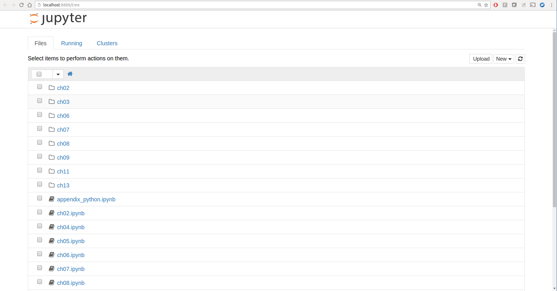
On many platforms, Jupyter will automatically open up in your
default web browser (unless you start it with
--no-browser). Otherwise, you can navigate to the
HTTP address printed when you started the notebook, here
http://localhost:8888/. See Figure 2-1 for what this looks like in Google
Chrome.
Many people use Jupyter as a local computing environment, but it can also be deployed on servers and accessed remotely. I won’t cover those details here, but encourage you to explore this topic on the internet if it’s relevant to your needs.
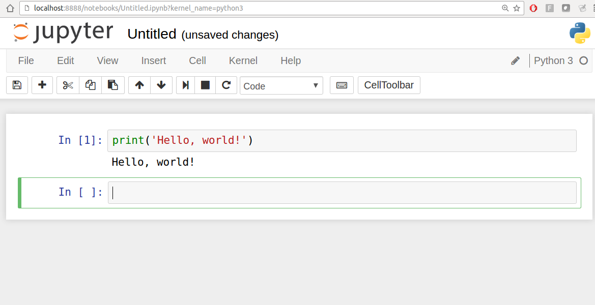
To create a new notebook, click the New button and select the “Python 3” or “conda [default]” option. You should see something like Figure 2-2. If this is your first time, try clicking on the empty code “cell” and entering a line of Python code. Then press Shift-Enter to execute it.
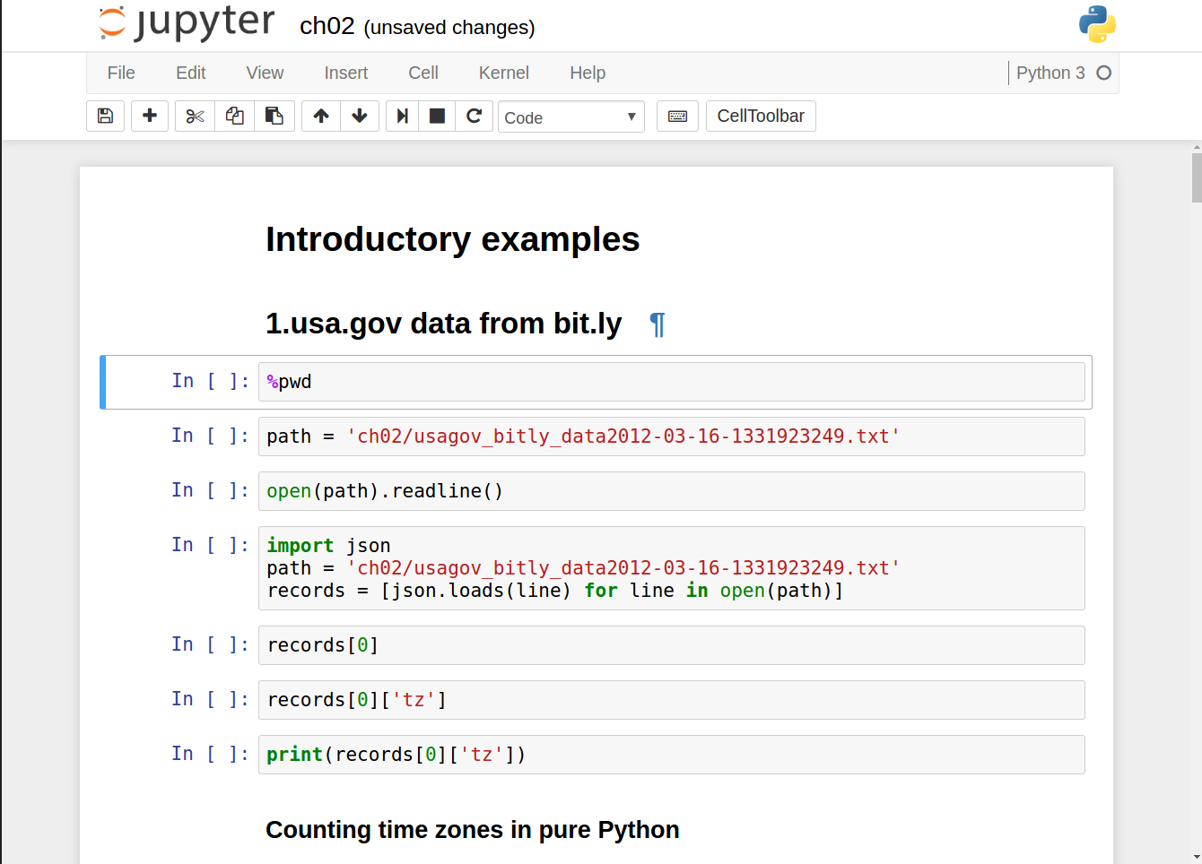
When you save the notebook (see “Save and Checkpoint” under the notebook File menu), it creates a file with the extension .ipynb. This is a self-contained file format that contains all of the content (including any evaluated code output) currently in the notebook. These can be loaded and edited by other Jupyter users. To load an existing notebook, put the file in the same directory where you started the notebook process (or in a subfolder within it), then double-click the name from the landing page. You can try it out with the notebooks from my wesm/pydata-book repository on GitHub. See Figure 2-3.
While the Jupyter notebook can feel like a distinct experience from the IPython shell, nearly all of the commands and tools in this chapter can be used in either environment.
On the surface, the IPython shell looks like a cosmetically different version
of the standard terminal Python interpreter (invoked with
python). One of the major improvements over the
standard Python shell is tab completion, found in
many IDEs or other interactive computing analysis environments. While
entering expressions in the shell, pressing the Tab key will search the
namespace for any variables (objects, functions, etc.) matching the
characters you have typed so far:
In [1]: an_apple = 27
In [2]: an_example = 42
In [3]: an<Tab>
an_apple and an_example anyIn this example, note that IPython displayed both the two
variables I defined as well as the Python keyword and and built-in function any.
Naturally, you can also complete methods and attributes on any object
after typing a period:
In [3]: b = [1, 2, 3]
In [4]: b.<Tab>
b.append b.count b.insert b.reverse
b.clear b.extend b.pop b.sort
b.copy b.index b.removeThe same goes for modules:
In [1]: import datetime
In [2]: datetime.<Tab>
datetime.date datetime.MAXYEAR datetime.timedelta
datetime.datetime datetime.MINYEAR datetime.timezone
datetime.datetime_CAPI datetime.time datetime.tzinfoIn the Jupyter notebook and newer versions of IPython (5.0 and higher), the autocompletions show up in a drop-down box rather than as text output.
Note that IPython by default hides methods and attributes starting with underscores, such as magic methods and internal “private” methods and attributes, in order to avoid cluttering the display (and confusing novice users!). These, too, can be tab-completed, but you must first type an underscore to see them. If you prefer to always see such methods in tab completion, you can change this setting in the IPython configuration. See the IPython documentation to find out how to do this.
Tab completion works in many contexts outside of searching the interactive namespace and completing object or module attributes. When typing anything that looks like a file path (even in a Python string), pressing the Tab key will complete anything on your computer’s filesystem matching what you’ve typed:
In [7]: datasets/movielens/<Tab>datasets/movielens/movies.dat datasets/movielens/README datasets/movielens/ratings.dat datasets/movielens/users.dat In [7]: path = 'datasets/movielens/<Tab>datasets/movielens/movies.dat datasets/movielens/README datasets/movielens/ratings.dat datasets/movielens/users.dat
Combined with the %run command
(see “The %run Command”), this functionality
can save you many keystrokes.
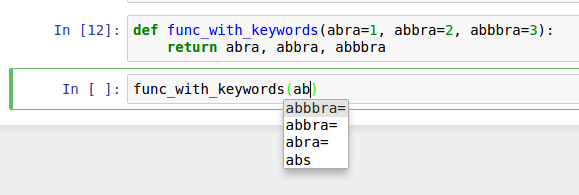
Another area where tab completion saves time is in the completion
of function keyword arguments (and including the = sign!). See Figure 2-4.
Using a question mark (?)
before or after a variable will display some general information about
the object:
In[8]:b=[1,2,3]In[9]:b?Type:listStringForm:[1,2,3]Length:3Docstring:list()->newemptylistlist(iterable)->newlistinitializedfromiterable's itemsIn[10]:?Docstring:(value,...,sep=' ',end='\n',file=sys.stdout,flush=False)Printsthevaluestoastream,ortosys.stdoutbydefault.Optionalkeywordarguments:file:afile-likeobject(stream);defaultstothecurrentsys.stdout.sep:stringinsertedbetweenvalues,defaultaspace.end:stringappendedafterthelastvalue,defaultanewline.flush:whethertoforciblyflushthestream.Type:builtin_function_or_method
This is referred to as object introspection. If the object is a function or instance method, the docstring, if defined, will also be shown. Suppose we’d written the following function (which you can reproduce in IPython or Jupyter):
defadd_numbers(a,b):"""Add two numbers togetherReturns-------the_sum : type of arguments"""returna+b
Then using ? shows us the
docstring:
In[11]:add_numbers?Signature:add_numbers(a,b)Docstring:AddtwonumberstogetherReturns-------the_sum:typeofargumentsFile:<ipython-input-9-6a548a216e27>Type:function
Using ?? will also show the
function’s source code if possible:
In[12]:add_numbers??Signature:add_numbers(a,b)Source:defadd_numbers(a,b):"""Add two numbers togetherReturns-------the_sum : type of arguments"""returna+bFile:<ipython-input-9-6a548a216e27>Type:function
? has a final usage, which is
for searching the IPython namespace in a manner similar to the standard
Unix or Windows command line. A number of characters combined with the wildcard (*) will show all names matching the wildcard expression. For
example, we could get a list of all functions in the top-level NumPy
namespace containing load:
In[13]:np.*load*?np.__loader__np.loadnp.loadsnp.loadtxtnp.pkgload
You can run any file as a Python program inside the environment of your
IPython session using the %run
command. Suppose you had the following simple script stored in
ipython_script_test.py:
deff(x,y,z):return(x+y)/za=5b=6c=7.5result=f(a,b,c)
You can execute this by passing the filename to %run:
In[14]:%runipython_script_test.py
The script is run in an empty namespace (with no imports
or other variables defined) so that the behavior should be identical to
running the program on the command line using python script.py. All of the variables
(imports, functions, and globals) defined in the file (up until an
exception, if any, is raised) will then be accessible in the IPython
shell:
In[15]:cOut[15]:7.5In[16]:resultOut[16]:1.4666666666666666
If a Python script expects command-line arguments (to be found in
sys.argv), these can be passed after
the file path as though run on the command line.
Should you wish to give a script access to variables already
defined in the interactive IPython namespace, use %run -i instead of plain %run.
In the Jupyter notebook, you may also use the related %load magic function, which
imports a script into a code cell:
>>>%loadipython_script_test.pydeff(x,y,z):return(x+y)/za=5b=6c=7.5result=f(a,b,c)
Pressing Ctrl-C while any code is running, whether a script through %run or a long-running command, will cause a
KeyboardInterrupt to be raised. This will cause nearly all Python programs to
stop immediately except in certain unusual cases.
When a piece of Python code has called into some compiled extension modules, pressing Ctrl-C will not always cause the program execution to stop immediately. In such cases, you will have to either wait until control is returned to the Python interpreter, or in more dire circumstances, forcibly terminate the Python process.
If you are using the Jupyter notebook, you can copy and paste code into any code cell and execute it. It is also possible to run code from the clipboard in the IPython shell. Suppose you had the following code in some other application:
x=5y=7ifx>5:x+=1y=8
The most foolproof methods are the %paste and
%cpaste magic functions. %paste takes whatever text is in the clipboard
and executes it as a single block in the shell:
In[17]:%pastex=5y=7ifx>5:x+=1y=8## -- End pasted text --
%cpaste is similar, except that
it gives you a special prompt for pasting code into:
In[18]:%cpastePastingcode;enter'--'aloneonthelinetostoporuseCtrl-D.:x=5:y=7:ifx>5::x+=1::y=8:--
With the %cpaste block, you
have the freedom to paste as much code as you like before executing it.
You might decide to use %cpaste in
order to look at the pasted code before executing it. If you
accidentally paste the wrong code, you can break out of the %cpaste prompt by pressing Ctrl-C.
IPython has many keyboard shortcuts for navigating the prompt (which will be familiar to users of the Emacs text editor or the Unix bash shell) and interacting with the shell’s command history. Table 2-1 summarizes some of the most commonly used shortcuts. See Figure 2-5 for an illustration of a few of these, such as cursor movement.
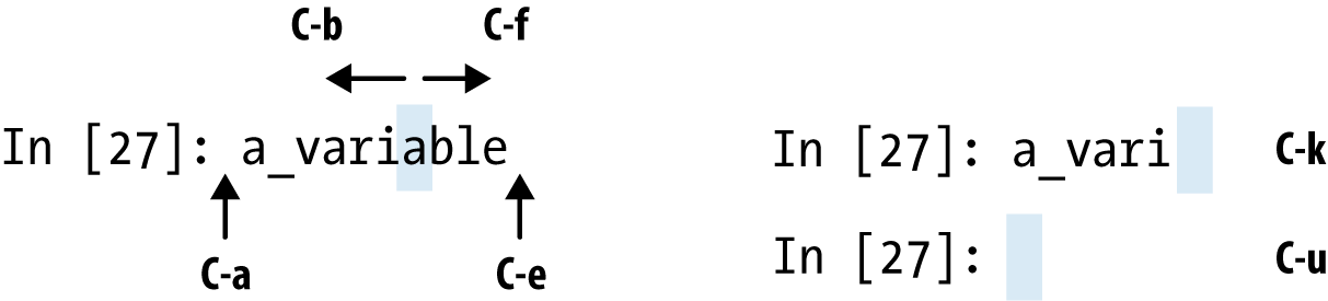
Note that Jupyter notebooks have a largely separate set of keyboard shortcuts for navigation and editing. Since these shortcuts have evolved more rapidly than IPython’s, I encourage you to explore the integrated help system in the Jupyter notebook’s menus.
IPython’s special commands (which are not built into Python itself) are known as
“magic” commands. These are designed to facilitate common tasks and
enable you to easily control the behavior of the IPython system. A magic
command is any command prefixed by the percent symbol %. For
example, you can check the execution time of any Python statement, such
as a matrix multiplication, using the %timeit magic function (which will be
discussed in more detail later):
In[20]:a=np.random.randn(100,100)In[20]:%timeitnp.dot(a,a)10000loops,bestof3:20.9µsperloop
Magic commands can be viewed as command-line programs to be run
within the IPython system. Many of them have additional “command-line”
options, which can all be viewed (as you might expect) using ?:
In[21]:%debug?Docstring:::%debug[--breakpointFILE:LINE][statement[statement...]]Activatetheinteractivedebugger.Thismagiccommandsupporttwowaysofactivatingdebugger.Oneistoactivatedebuggerbeforeexecutingcode.Thisway,youcansetabreakpoint,tostepthroughthecodefromthepoint.Youcanusethismodebygivingstatementstoexecuteandoptionallyabreakpoint.Theotheroneistoactivatedebuggerinpost-mortemmode.Youcanactivatethismodesimplyrunning%debugwithoutanyargument.Ifanexceptionhasjustoccurred,thisletsyouinspectitsstackframesinteractively.Notethatthiswillalwaysworkonlyonthelasttracebackthatoccurred,soyoumustcallthisquicklyafteranexceptionthatyouwishtoinspecthasfired,becauseifanotheroneoccurs,itclobbersthepreviousone.IfyouwantIPythontoautomaticallydothisoneveryexception,seethe%pdbmagicformoredetails.positionalarguments:statementCodetorunindebugger.Youcanomitthisincellmagicmode.optionalarguments:--breakpoint<FILE:LINE>,-b<FILE:LINE>SetbreakpointatLINEinFILE.
Magic functions can be used by default without the percent sign,
as long as no variable is defined with the same name as the magic
function in question. This feature is called automagic and can be
enabled or disabled with %automagic.
Some magic functions behave like Python functions and their output can be assigned to a variable:
In[22]:%pwdOut[22]:'/home/wesm/code/pydata-bookIn[23]:foo=%pwdIn[24]:fooOut[24]:'/home/wesm/code/pydata-book'
Since IPython’s documentation is accessible from within the
system, I encourage you to explore all of the special commands available
by typing %quickref or %magic. Table 2-2
highlights some of the most critical ones for being productive in
interactive computing and Python development in IPython.
One reason for IPython’s popularity in analytical computing is that it
integrates well with data visualization and other user interface
libraries like matplotlib. Don’t worry if you have never used matplotlib
before; it will be discussed in more detail later in this book.
The %matplotlib magic function
configures its integration with the IPython shell or Jupyter notebook.
This is important, as otherwise plots you create will either not appear
(notebook) or take control of the session until closed (shell).
In the IPython shell, running %matplotlib sets
up the integration so you can create multiple plot windows without
interfering with the console session:
In[26]:%matplotlibUsingmatplotlibbackend:Qt4Agg
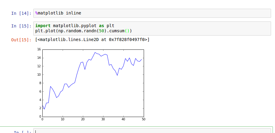
In Jupyter, the command is a little different (Figure 2-6):
In[26]:%matplotlibinline
In this section, I will give you an overview of essential Python programming concepts and language mechanics. In the next chapter, I will go into more detail about Python’s data structures, functions, and other built-in tools.
The Python language design is distinguished by its emphasis on readability, simplicity, and explicitness. Some people go so far as to liken it to “executable pseudocode.”
Python uses whitespace (tabs or spaces) to structure code instead of
using braces as in many other languages like R, C++, Java, and Perl.
Consider a for loop from a sorting
algorithm:
forxinarray:ifx<pivot:less.append(x)else:greater.append(x)
A colon denotes the start of an indented code block after which all of the code must be indented by the same amount until the end of the block.
Love it or hate it, significant whitespace is a fact of life for Python programmers, and in my experience it can make Python code more readable than other languages I’ve used. While it may seem foreign at first, you will hopefully grow accustomed in time.
I strongly recommend using four spaces as your default indentation and replacing tabs with four spaces. Many text editors have a setting that will replace tab stops with spaces automatically (do this!). Some people use tabs or a different number of spaces, with two spaces not being terribly uncommon. By and large, four spaces is the standard adopted by the vast majority of Python programmers, so I recommend doing that in the absence of a compelling reason otherwise.
As you can see by now, Python statements also do not need to be terminated by semicolons. Semicolons can be used, however, to separate multiple statements on a single line:
a = 5; b = 6; c = 7
Putting multiple statements on one line is generally discouraged in Python as it often makes code less readable.
An important characteristic of the Python language is the consistency of its object model. Every number, string, data structure, function, class, module, and so on exists in the Python interpreter in its own “box,” which is referred to as a Python object. Each object has an associated type (e.g., string or function) and internal data. In practice this makes the language very flexible, as even functions can be treated like any other object.
Any text preceded by the hash mark (pound sign) #
is ignored by the Python interpreter. This is often used to add
comments to code. At times you may also want to exclude certain blocks
of code without deleting them. An easy solution is to
comment out the code:
results=[]forlineinfile_handle:# keep the empty lines for now# if len(line) == 0:# continueresults.append(line.replace('foo','bar'))
Comments can also occur after a line of executed code. While some programmers prefer comments to be placed in the line preceding a particular line of code, this can be useful at times:
("Reached this line")# Simple status report
You call functions using parentheses and passing zero or more arguments, optionally assigning the returned value to a variable:
result=f(x,y,z)g()
Almost every object in Python has attached functions, known as methods, that have access to the object’s internal contents. You can call them using the following syntax:
obj.some_method(x,y,z)
Functions can take both positional and keyword arguments:
result=f(a,b,c,d=5,e='foo')
When assigning a variable (or name) in Python, you are creating a reference to the object on the righthand side of the equals sign. In practical terms, consider a list of integers:
In[8]:a=[1,2,3]
Suppose we assign a to a new
variable b:
In[9]:b=a
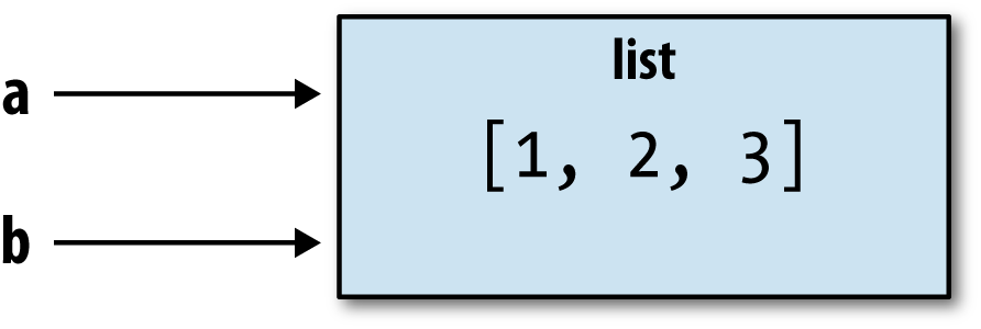
In some languages, this assignment would cause the data [1, 2, 3] to be copied. In Python, a and b
actually now refer to the same object, the original list [1, 2, 3] (see Figure 2-7 for a mockup). You can prove this to
yourself by appending an element to a and then examining b:
In[10]:a.append(4)In[11]:bOut[11]:[1,2,3,4]
Understanding the semantics of references in Python and when, how, and why data is copied is especially critical when you are working with larger datasets in Python.
Assignment is also referred to as binding, as we are binding a name to an object. Variable names that have been assigned may occasionally be referred to as bound variables.
When you pass objects as arguments to a function, new local variables are created referencing the original objects without any copying. If you bind a new object to a variable inside a function, that change will not be reflected in the parent scope. It is therefore possible to alter the internals of a mutable argument. Suppose we had the following function:
defappend_element(some_list,element):some_list.append(element)
Then we have:
In[27]:data=[1,2,3]In[28]:append_element(data,4)In[29]:dataOut[29]:[1,2,3,4]
In contrast with many compiled languages, such as Java and C++, object references in Python have no type associated with them. There is no problem with the following:
In[12]:a=5In[13]:type(a)Out[13]:intIn[14]:a='foo'In[15]:type(a)Out[15]:str
Variables are names for objects within a particular namespace; the type information is stored in the object itself. Some observers might hastily conclude that Python is not a “typed language.” This is not true; consider this example:
In[16]:'5'+5---------------------------------------------------------------------------TypeErrorTraceback(mostrecentcalllast)<ipython-input-16-4dd8efb5fac1>in<module>()---->1'5'+5TypeError:mustbestr,notint
In some languages, such as Visual Basic, the string '5' might get implicitly converted (or
casted) to an integer, thus yielding 10. Yet in
other languages, such as JavaScript, the integer 5 might be casted to a string, yielding the
concatenated string '55'. In this
regard Python is considered a strongly typed
language, which means that every object has a specific type (or
class), and implicit conversions will occur only
in certain obvious circumstances, such as the following:
In[17]:a=4.5In[18]:b=2# String formatting, to be visited laterIn[19]:('a is {0}, b is {1}'.format(type(a),type(b)))ais<class'float'>, b is <class 'int'>In[20]:a/bOut[20]:2.25
Knowing the type of an object is important, and it’s useful to
be able to write functions that can handle many different kinds of
input. You can check that an object is an instance of a particular
type using the isinstance
function:
In[21]:a=5In[22]:isinstance(a,int)Out[22]:True
isinstance can accept a tuple
of types if you want to check that an object’s type is among those
present in the tuple:
In[23]:a=5;b=4.5In[24]:isinstance(a,(int,float))Out[24]:TrueIn[25]:isinstance(b,(int,float))Out[25]:True
Objects in Python typically have both attributes (other Python objects
stored “inside” the object) and methods (functions associated with an
object that can have access to the object’s internal data). Both of
them are accessed via the syntax
obj.attribute_name:
In[1]:a='foo'In[2]:a.<PressTab>a.capitalizea.formata.isuppera.rindexa.stripa.centera.indexa.joina.rjusta.swapcasea.counta.isalnuma.ljusta.rpartitiona.titlea.decodea.isalphaa.lowera.rsplita.translatea.encodea.isdigita.lstripa.rstripa.uppera.endswitha.islowera.partitiona.splita.zfilla.expandtabsa.isspacea.replacea.splitlinesa.finda.istitlea.rfinda.startswith
Attributes and methods can also be accessed by name via
the getattr
function:
In[27]:getattr(a,'split')Out[27]:<functionstr.split>
In other languages, accessing objects by name is often referred
to as “reflection.” While we will not extensively use the functions
getattr and related functions hasattr and
setattr in this book, they can be
used very effectively to write generic, reusable code.
Often you may not care about the type of an object but rather only whether it
has certain methods or behavior. This is sometimes called “duck
typing,” after the saying “If it walks like a duck and quacks like a
duck, then it’s a duck.” For example, you can verify that an object is
iterable if it implemented the iterator protocol. For many
objects, this means it has a __iter__
“magic method,” though an alternative and better way to check is to
try using the iter
function:
defisiterable(obj):try:iter(obj)returnTrueexceptTypeError:# not iterablereturnFalse
This function would return True for strings as well as most Python
collection types:
In[29]:isiterable('a string')Out[29]:TrueIn[30]:isiterable([1,2,3])Out[30]:TrueIn[31]:isiterable(5)Out[31]:False
A place where I use this functionality all the time is to write functions that can accept multiple kinds of input. A common case is writing a function that can accept any kind of sequence (list, tuple, ndarray) or even an iterator. You can first check if the object is a list (or a NumPy array) and, if it is not, convert it to be one:
ifnotisinstance(x,list)andisiterable(x):x=list(x)
In Python a module is simply a file with the .py extension containing Python code. Suppose that we had the following module:
# some_module.pyPI=3.14159deff(x):returnx+2defg(a,b):returna+b
If we wanted to access the variables and functions defined in some_module.py, from another file in the same directory we could do:
importsome_moduleresult=some_module.f(5)pi=some_module.PI
Or equivalently:
fromsome_moduleimportf,g,PIresult=g(5,PI)
By using the as keyword
you can give imports different variable names:
importsome_moduleassmfromsome_moduleimportPIaspi,gasgfr1=sm.f(pi)r2=gf(6,pi)
Most of the binary math operations and comparisons are as you might expect:
In[32]:5-7Out[32]:-2In[33]:12+21.5Out[33]:33.5In[34]:5<=2Out[34]:False
See Table 2-3 for all of the available binary operators.
To check if two references refer to the same object, use the
is keyword. is not is also perfectly valid if you want
to check that two objects are not the same:
In[35]:a=[1,2,3]In[36]:b=aIn[37]:c=list(a)In[38]:aisbOut[38]:TrueIn[39]:aisnotcOut[39]:True
Since list always creates a new Python list (i.e., a copy), we can be sure
that c is distinct from a.
Comparing with is is not the same as the == operator, because in this case we
have:
In[40]:a==cOut[40]:True
A very common use of is and
is not is to check if a variable is
None, since there is only one
instance of None:
In[41]:a=NoneIn[42]:aisNoneOut[42]:True
Most objects in Python, such as lists, dicts, NumPy arrays, and most user-defined types (classes), are mutable. This means that the object or values that they contain can be modified:
In[43]:a_list=['foo',2,[4,5]]In[44]:a_list[2]=(3,4)In[45]:a_listOut[45]:['foo',2,(3,4)]
Others, like strings and tuples, are immutable:
In[46]:a_tuple=(3,5,(4,5))In[47]:a_tuple[1]='four'---------------------------------------------------------------------------TypeErrorTraceback(mostrecentcalllast)<ipython-input-47-23fe12da1ba6>in<module>()---->1a_tuple[1]='four'TypeError:'tuple'objectdoesnotsupportitemassignment
Remember that just because you can mutate an object does not mean that you always should. Such actions are known as side effects. For example, when writing a function, any side effects should be explicitly communicated to the user in the function’s documentation or comments. If possible, I recommend trying to avoid side effects and favor immutability, even though there may be mutable objects involved.
Python along with its standard library has a small set of built-in types for
handling numerical data, strings, boolean (True or False) values, and dates and time. These
“single value” types are sometimes called scalar
types and we refer to them in this book as scalars. See Table 2-4 for a list of the main scalar
types. Date and time handling will be discussed separately, as these are
provided by the datetime module in
the standard library.
The primary Python types for numbers are int and float. An int can store
arbitrarily large numbers:
In[48]:ival=17239871In[49]:ival**6Out[49]:26254519291092456596965462913230729701102721
Floating-point numbers are represented with the Python float type. Under the hood each one is a
double-precision (64-bit) value. They can also be expressed with
scientific notation:
In[50]:fval=7.243In[51]:fval2=6.78e-5
Integer division not resulting in a whole number will always yield a floating-point number:
In[52]:3/2Out[52]:1.5
To get C-style integer division (which drops the fractional part
if the result is not a whole number), use the floor division
operator //:
In[53]:3//2Out[53]:1
Many people use Python for its powerful and flexible built-in string
processing capabilities. You can write string
literals using either single quotes ' or double
quotes ":
a='one way of writing a string'b="another way"
For multiline strings with line breaks, you can use triple
quotes, either ''' or """:
c="""This is a longer string thatspans multiple lines"""
It may surprise you that this string c
actually contains four lines of text; the line breaks after
""" and after lines are included
in the string. We can count the new line characters with the count method on
c:
In[55]:c.count('\n')Out[55]:3
Python strings are immutable; you cannot modify a string:
In[56]:a='this is a string'In[57]:a[10]='f'---------------------------------------------------------------------------TypeErrorTraceback(mostrecentcalllast)<ipython-input-57-2151a30ed055>in<module>()---->1a[10]='f'TypeError:'str'objectdoesnotsupportitemassignmentIn[58]:b=a.replace('string','longer string')In[59]:bOut[59]:'this is a longer string'
Afer this operation, the variable a is
unmodified:
In[60]:aOut[60]:'this is a string'
Many Python objects can be converted to a string using the str
function:
In[61]:a=5.6In[62]:s=str(a)In[63]:(s)5.6
Strings are a sequence of Unicode characters and therefore can be treated like other sequences, such as lists and tuples (which we will explore in more detail in the next chapter):
In[64]:s='python'In[65]:list(s)Out[65]:['p','y','t','h','o','n']In[66]:s[:3]Out[66]:'pyt'
The syntax s[:3] is called
slicing and is implemented for many kinds of Python sequences.
This will be explained in more detail later on, as it is used
extensively in this book.
The backslash character \
is an escape character, meaning that it is used
to specify special characters like newline \n or Unicode characters. To write a string
literal with backslashes, you need to escape them:
In[67]:s='12\\34'In[68]:(s)12\34
If you have a string with a lot of backslashes and no special
characters, you might find this a bit annoying. Fortunately you can
preface the leading quote of the string with r, which
means that the characters should be interpreted as is:
In[69]:s=r'this\has\no\special\characters'In[70]:sOut[70]:'this\\has\\no\\special\\characters'
The r stands for
raw.
Adding two strings together concatenates them and produces a new string:
In[71]:a='this is the first half 'In[72]:b='and this is the second half'In[73]:a+bOut[73]:'this is the first half and this is the second half'
String templating or formatting is another important topic. The number of
ways to do so has expanded with the advent of Python 3, and here I will
briefly describe the mechanics of one of the main interfaces. String
objects have a format method that can be
used to substitute formatted arguments into the string, producing a
new string:
In[74]:template='{0:.2f} {1:s} are worth US${2:d}'
In this string,
{0:.2f} means to format
the first argument as a floating-point number with two decimal
places.
{1:s} means to format the
second argument as a string.
{2:d} means to format the
third argument as an exact integer.
To substitute arguments for these format parameters, we pass a
sequence of arguments to the format method:
In[75]:template.format(4.5560,'Argentine Pesos',1)Out[75]:'4.56 Argentine Pesos are worth US$1'
String formatting is a deep topic; there are multiple methods and numerous options and tweaks available to control how values are formatted in the resulting string. To learn more, I recommend consulting the official Python documentation.
I discuss general string processing as it relates to data analysis in more detail in Chapter 8.
In modern Python (i.e., Python 3.0 and up), Unicode has become the first-class string type to enable more consistent handling of ASCII and non-ASCII text. In older versions of Python, strings were all bytes without any explicit Unicode encoding. You could convert to Unicode assuming you knew the character encoding. Let’s look at an example:
In[76]:val="español"In[77]:valOut[77]:'español'
We can convert this Unicode string to its UTF-8 bytes
representation using the encode method:
In[78]:val_utf8=val.encode('utf-8')In[79]:val_utf8Out[79]:b'espa\xc3\xb1ol'In[80]:type(val_utf8)Out[80]:bytes
Assuming you know the Unicode encoding of a bytes object, you
can go back using the decode method:
In[81]:val_utf8.decode('utf-8')Out[81]:'español'
While it’s become preferred to use UTF-8 for any encoding, for historical reasons you may encounter data in any number of different encodings:
In[82]:val.encode('latin1')Out[82]:b'espa\xf1ol'In[83]:val.encode('utf-16')Out[83]:b'\xff\xfee\x00s\x00p\x00a\x00\xf1\x00o\x00l\x00'In[84]:val.encode('utf-16le')Out[84]:b'e\x00s\x00p\x00a\x00\xf1\x00o\x00l\x00'
It is most common to encounter bytes objects in the
context of working with files, where implicitly decoding all data to
Unicode strings may not be desired.
Though you may seldom need to do so, you can define your own
byte literals by prefixing a string with b:
In[85]:bytes_val=b'this is bytes'In[86]:bytes_valOut[86]:b'this is bytes'In[87]:decoded=bytes_val.decode('utf8')In[88]:decoded# this is str (Unicode) nowOut[88]:'this is bytes'
None is the Python null value type. If a function does not explicitly
return a value, it implicitly returns None:
In[97]:a=NoneIn[98]:aisNoneOut[98]:TrueIn[99]:b=5In[100]:bisnotNoneOut[100]:True
None is also a common default
value for function arguments:
defadd_and_maybe_multiply(a,b,c=None):result=a+bifcisnotNone:result=result*creturnresult
While a technical point, it’s worth bearing in mind that
None is not only a reserved keyword
but also a unique instance of NoneType:
In[101]:type(None)Out[101]:NoneType
The built-in Python datetime
module provides datetime,
date, and time types. The datetime type, as you may imagine, combines
the information stored in date and
time and is the most commonly
used:
In[102]:fromdatetimeimportdatetime,date,timeIn[103]:dt=datetime(2011,10,29,20,30,21)In[104]:dt.dayOut[104]:29In[105]:dt.minuteOut[105]:30
Given a datetime instance,
you can extract the equivalent date
and time objects by calling methods
on the datetime of the same
name:
In[106]:dt.date()Out[106]:datetime.date(2011,10,29)In[107]:dt.time()Out[107]:datetime.time(20,30,21)
The strftime method
formats a datetime as a
string:
In[108]:dt.strftime('%m/%d/%Y%H:%M')Out[108]:'10/29/2011 20:30'
Strings can be converted (parsed) into
datetime objects with the strptime
function:
In[109]:datetime.strptime('20091031','%Y%m%d')Out[109]:datetime.datetime(2009,10,31,0,0)
See Table 2-5 for a full list of format specifications.
When you are aggregating or otherwise grouping time series data, it will
occasionally be useful to replace time fields of a series of
datetimes—for example, replacing the minute and
second fields with zero:
In[110]:dt.replace(minute=0,second=0)Out[110]:datetime.datetime(2011,10,29,20,0)
Since datetime.datetime is an immutable type,
methods like these always produce new objects.
The difference of two datetime objects
produces a datetime.timedelta
type:
In[111]:dt2=datetime(2011,11,15,22,30)In[112]:delta=dt2-dtIn[113]:deltaOut[113]:datetime.timedelta(17,7179)In[114]:type(delta)Out[114]:datetime.timedelta
The output timedelta(17, 7179) indicates that
the timedelta encodes an offset of 17 days and 7,179 seconds.
Adding a timedelta to a
datetime produces a new shifted
datetime:
In[115]:dtOut[115]:datetime.datetime(2011,10,29,20,30,21)In[116]:dt+deltaOut[116]:datetime.datetime(2011,11,15,22,30)
Python has several built-in keywords for conditional logic, loops, and other standard control flow concepts found in other programming languages.
The if statement is one of the most well-known control flow statement
types. It checks a condition that, if True, evaluates the code in the block that
follows:
ifx<0:('It'snegative')
An if statement can be
optionally followed by one or more elif blocks and
a catch-all else block if all of the conditions are False:
ifx<0:('It'snegative')elifx==0:('Equal to zero')elif0<x<5:('Positive but smaller than 5')else:('Positive and larger than or equal to 5')
If any of the conditions is True, no further elif or else blocks will be reached. With a compound
condition using and or or, conditions are evaluated left to right
and will short-circuit:
In[117]:a=5;b=7In[118]:c=8;d=4In[119]:ifa<borc>d:.....:('Made it')Madeit
In this example, the comparison c >
d never gets evaluated because the first comparison was
True.
It is also possible to chain comparisons:
In[120]:4>3>2>1Out[120]:True
for loops are for iterating over a collection (like a list or tuple) or
an iterater. The standard syntax for a for loop is:
forvalueincollection:# do something with value
You can advance a for loop to
the next iteration, skipping the remainder of the block, using the
continue keyword. Consider this code, which sums up integers in a list and
skips None values:
sequence=[1,2,None,4,None,5]total=0forvalueinsequence:ifvalueisNone:continuetotal+=value
A for loop can be exited
altogether with the break keyword.
This code sums elements of the list until a 5 is reached:
sequence=[1,2,0,4,6,5,2,1]total_until_5=0forvalueinsequence:ifvalue==5:breaktotal_until_5+=value
The break keyword only terminates the
innermost for loop; any outer
for loops will continue to run:
In[121]:foriinrange(4):.....:forjinrange(4):.....:ifj>i:.....:break.....:((i,j)).....:(0,0)(1,0)(1,1)(2,0)(2,1)(2,2)(3,0)(3,1)(3,2)(3,3)
As we will see in more detail, if the elements in the collection
or iterator are sequences (tuples or lists, say), they can be
conveniently unpacked into variables in the
for loop statement:
fora,b,ciniterator:# do something
pass is the “no-op” statement
in Python. It can be used in blocks where no action is
to be taken (or as a placeholder for code not yet implemented); it is
only required because Python uses whitespace to delimit blocks:
ifx<0:('negative!')elifx==0:# TODO: put something smart herepasselse:('positive!')
The range function returns an iterator that yields a sequence of evenly
spaced integers:
In[122]:range(10)Out[122]:range(0,10)In[123]:list(range(10))Out[123]:[0,1,2,3,4,5,6,7,8,9]
Both a start, end, and step (which may be negative) can be given:
In[124]:list(range(0,20,2))Out[124]:[0,2,4,6,8,10,12,14,16,18]In[125]:list(range(5,0,-1))Out[125]:[5,4,3,2,1]
As you can see, range
produces integers up to but not including the endpoint. A common use
of range is for iterating through
sequences by index:
seq=[1,2,3,4]foriinrange(len(seq)):val=seq[i]
While you can use functions like list to
store all the integers generated by range in some
other data structure, often the default iterator form will be what you
want. This snippet sums all numbers from 0 to 99,999 that are
multiples of 3 or 5:
sum=0foriinrange(100000):# % is the modulo operatorifi%3==0ori%5==0:sum+=i
While the range generated can be arbitrarily large, the memory use at any given time may be very small.
A ternary expression in Python allows you to combine an if-else block that produces a value into a
single line or expression. The syntax for this in Python is:
value =true-exprif condition elsefalse-expr
Here, true-expr and
false-expr can be any Python expressions.
It has the identical effect as the more verbose:
ifcondition: value =true-exprelse: value =false-expr
This is a more concrete example:
In[126]:x=5In[127]:'Non-negative'ifx>=0else'Negative'Out[127]:'Non-negative'
As with if-else blocks, only
one of the expressions will be executed. Thus, the “if” and “else”
sides of the ternary expression could contain costly computations, but
only the true branch is ever evaluated.
While it may be tempting to always use ternary expressions to condense your code, realize that you may sacrifice readability if the condition as well as the true and false expressions are very complex.
This chapter discusses capabilities built into the Python language that will be used ubiquitously throughout the book. While add-on libraries like pandas and NumPy add advanced computational functionality for larger datasets, they are designed to be used together with Python’s built-in data manipulation tools.
We’ll start with Python’s workhorse data structures: tuples, lists, dicts, and sets. Then, we’ll discuss creating your own reusable Python functions. Finally, we’ll look at the mechanics of Python file objects and interacting with your local hard drive.
Python’s data structures are simple but powerful. Mastering their use is a critical part of becoming a proficient Python programmer.
A tuple is a fixed-length, immutable sequence of Python objects. The easiest way to create one is with a comma-separated sequence of values:
In[1]:tup=4,5,6In[2]:tupOut[2]:(4,5,6)
When you’re defining tuples in more complicated expressions, it’s often necessary to enclose the values in parentheses, as in this example of creating a tuple of tuples:
In[3]:nested_tup=(4,5,6),(7,8)In[4]:nested_tupOut[4]:((4,5,6),(7,8))
You can convert any sequence or iterator to a tuple by invoking
tuple:
In[5]:tuple([4,0,2])Out[5]:(4,0,2)In[6]:tup=tuple('string')In[7]:tupOut[7]:('s','t','r','i','n','g')
Elements can be accessed with square brackets [] as
with most other sequence types. As in C, C++, Java, and many other
languages, sequences are 0-indexed in Python:
In[8]:tup[0]Out[8]:'s'
While the objects stored in a tuple may be mutable themselves, once the tuple is created it’s not possible to modify which object is stored in each slot:
In[9]:tup=tuple(['foo',[1,2],True])In[10]:tup[2]=False---------------------------------------------------------------------------TypeErrorTraceback(mostrecentcalllast)<ipython-input-10-b89d0c4ae599>in<module>()---->1tup[2]=FalseTypeError:'tuple'objectdoesnotsupportitemassignment
If an object inside a tuple is mutable, such as a list, you can modify it in-place:
In[11]:tup[1].append(3)In[12]:tupOut[12]:('foo',[1,2,3],True)
You can concatenate tuples using the + operator to
produce longer tuples:
In[13]:(4,None,'foo')+(6,0)+('bar',)Out[13]:(4,None,'foo',6,0,'bar')
Multiplying a tuple by an integer, as with lists, has the effect of concatenating together that many copies of the tuple:
In[14]:('foo','bar')*4Out[14]:('foo','bar','foo','bar','foo','bar','foo','bar')
Note that the objects themselves are not copied, only the references to them.
If you try to assign to a tuple-like expression of variables, Python will attempt to unpack the value on the righthand side of the equals sign:
In[15]:tup=(4,5,6)In[16]:a,b,c=tupIn[17]:bOut[17]:5
Even sequences with nested tuples can be unpacked:
In[18]:tup=4,5,(6,7)In[19]:a,b,(c,d)=tupIn[20]:dOut[20]:7
Using this functionality you can easily swap variable names, a task which in many languages might look like:
tmp=aa=bb=tmp
But, in Python, the swap can be done like this:
In[21]:a,b=1,2In[22]:aOut[22]:1In[23]:bOut[23]:2In[24]:b,a=a,bIn[25]:aOut[25]:2In[26]:bOut[26]:1
A common use of variable unpacking is iterating over sequences of tuples or lists:
In[27]:seq=[(1,2,3),(4,5,6),(7,8,9)]In[28]:fora,b,cinseq:....:('a={0}, b={1}, c={2}'.format(a,b,c))a=1,b=2,c=3a=4,b=5,c=6a=7,b=8,c=9
Another common use is returning multiple values from a function. I’ll cover this in more detail later.
The Python language recently acquired some more advanced tuple
unpacking to help with situations where you may want to “pluck” a few
elements from the beginning of a tuple. This uses the special syntax
*rest, which is also used in function signatures to capture an arbitrarily
long list of positional arguments:
In[29]:values=1,2,3,4,5In[30]:a,b,*rest=valuesIn[31]:a,bOut[31]:(1,2)In[32]:restOut[32]:[3,4,5]
This rest bit is sometimes something you want
to discard; there is nothing special about the rest
name. As a matter of convention, many Python programmers will use the
underscore (_) for unwanted
variables:
In[33]:a,b,*_=values
In contrast with tuples, lists are variable-length and their contents
can be modified in-place. You can define them using square brackets
[] or using the list type
function:
In[36]:a_list=[2,3,7,None]In[37]:tup=('foo','bar','baz')In[38]:b_list=list(tup)In[39]:b_listOut[39]:['foo','bar','baz']In[40]:b_list[1]='peekaboo'In[41]:b_listOut[41]:['foo','peekaboo','baz']
Lists and tuples are semantically similar (though tuples cannot be modified) and can be used interchangeably in many functions.
The list function is frequently used in data
processing as a way to materialize an iterator or generator
expression:
In[42]:gen=range(10)In[43]:genOut[43]:range(0,10)In[44]:list(gen)Out[44]:[0,1,2,3,4,5,6,7,8,9]
Elements can be appended to the end of the list with the append
method:
In[45]:b_list.append('dwarf')In[46]:b_listOut[46]:['foo','peekaboo','baz','dwarf']
Using insert you can
insert an element at a specific location in the
list:
In[47]:b_list.insert(1,'red')In[48]:b_listOut[48]:['foo','red','peekaboo','baz','dwarf']
The insertion index must be between 0 and the length of the list, inclusive.
insert is computationally
expensive compared with append,
because references to subsequent elements have to be shifted
internally to make room for the new element. If you need to insert
elements at both the beginning and end of a sequence, you may
wish to explore collections.deque,
a double-ended queue, for this purpose.
The inverse operation to insert is pop, which removes and returns an element at a particular
index:
In[49]:b_list.pop(2)Out[49]:'peekaboo'In[50]:b_listOut[50]:['foo','red','baz','dwarf']
Elements can be removed by value with remove, which
locates the first such value and removes it from the last:
In[51]:b_list.append('foo')In[52]:b_listOut[52]:['foo','red','baz','dwarf','foo']In[53]:b_list.remove('foo')In[54]:b_listOut[54]:['red','baz','dwarf','foo']
If performance is not a concern, by using append and remove, you can use a Python list as a
perfectly suitable “multiset” data structure.
Check if a list contains a value using the in
keyword:
In[55]:'dwarf'inb_listOut[55]:True
The keyword not can be used to negate
in:
In[56]:'dwarf'notinb_listOut[56]:False
Checking whether a list contains a value is a lot slower than doing so with dicts and sets (to be introduced shortly), as Python makes a linear scan across the values of the list, whereas it can check the others (based on hash tables) in constant time.
Similar to tuples, adding two lists together with + concatenates
them:
In[57]:[4,None,'foo']+[7,8,(2,3)]Out[57]:[4,None,'foo',7,8,(2,3)]
If you have a list already defined, you can append multiple
elements to it using the extend
method:
In[58]:x=[4,None,'foo']In[59]:x.extend([7,8,(2,3)])In[60]:xOut[60]:[4,None,'foo',7,8,(2,3)]
Note that list concatenation by addition is a comparatively
expensive operation since a new list must be created and the objects
copied over. Using extend to append
elements to an existing list, especially if you are building up a
large list, is usually preferable. Thus,
everything=[]forchunkinlist_of_lists:everything.extend(chunk)
is faster than the concatenative alternative:
everything=[]forchunkinlist_of_lists:everything=everything+chunk
You can sort a list in-place (without creating a new object) by
calling its sort
function:
In[61]:a=[7,2,5,1,3]In[62]:a.sort()In[63]:aOut[63]:[1,2,3,5,7]
sort has a few options that
will occasionally come in handy. One is the ability to pass a
secondary sort key—that is, a function that
produces a value to use to sort the objects. For example, we could
sort a collection of strings by their lengths:
In[64]:b=['saw','small','He','foxes','six']In[65]:b.sort(key=len)In[66]:bOut[66]:['He','saw','six','small','foxes']
Soon, we’ll look at the sorted function, which can
produce a sorted copy of a general sequence.
The built-in bisect module
implements binary search and insertion into a sorted
list. bisect.bisect finds the location where an element should be inserted to
keep it sorted, while bisect.insort
actually inserts the element into that location:
In[67]:importbisectIn[68]:c=[1,2,2,2,3,4,7]In[69]:bisect.bisect(c,2)Out[69]:4In[70]:bisect.bisect(c,5)Out[70]:6In[71]:bisect.insort(c,6)In[72]:cOut[72]:[1,2,2,2,3,4,6,7]
The bisect module functions
do not check whether the list is sorted, as doing so would be
computationally expensive. Thus, using them with an unsorted list
will succeed without error but may lead to incorrect results.
You can select sections of most sequence types by using slice notation, which in its basic form consists of
start:stop passed to the indexing
operator []:
In[73]:seq=[7,2,3,7,5,6,0,1]In[74]:seq[1:5]Out[74]:[2,3,7,5]
Slices can also be assigned to with a sequence:
In[75]:seq[3:4]=[6,3]In[76]:seqOut[76]:[7,2,3,6,3,5,6,0,1]
While the element at the start index is
included, the stop index is
not included, so that the number of elements in
the result is stop - start.
Either the start or stop can be omitted, in which case they
default to the start of the sequence and the end of the sequence,
respectively:
In[77]:seq[:5]Out[77]:[7,2,3,6,3]In[78]:seq[3:]Out[78]:[6,3,5,6,0,1]
Negative indices slice the sequence relative to the end:
In[79]:seq[-4:]Out[79]:[5,6,0,1]In[80]:seq[-6:-2]Out[80]:[6,3,5,6]
Slicing semantics takes a bit of getting used to, especially if you’re coming from R or MATLAB. See Figure 3-1 for a helpful illustration of slicing with positive and negative integers. In the figure, the indices are shown at the “bin edges” to help show where the slice selections start and stop using positive or negative indices.
A step can also be used after a second colon to, say, take every
other element:
In[81]:seq[::2]Out[81]:[7,3,3,6,1]
A clever use of this is to pass -1, which has the useful effect of reversing
a list or tuple:
In[82]:seq[::-1]Out[82]:[1,0,6,5,3,6,3,2,7]
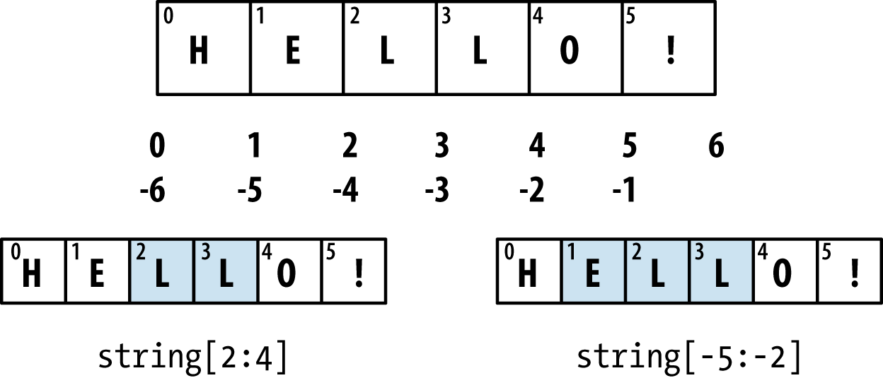
Python has a handful of useful sequence functions that you should familiarize yourself with and use at any opportunity.
It’s common when iterating over a sequence to want to keep track of the index of the current item. A do-it-yourself approach would look like:
i=0forvalueincollection:# do something with valuei+=1
Since this is so common, Python has a built-in function, enumerate, which returns a sequence of
(i, value) tuples:
fori,valueinenumerate(collection):# do something with value
When you are indexing data, a helpful pattern that uses enumerate is computing a dict mapping the values of a sequence (which
are assumed to be unique) to their locations in the sequence:
In[83]:some_list=['foo','bar','baz']In[84]:mapping={}In[85]:fori,vinenumerate(some_list):....:mapping[v]=iIn[86]:mappingOut[86]:{'bar':1,'baz':2,'foo':0}
The sorted function returns
a new sorted list from the elements of any
sequence:
In[87]:sorted([7,1,2,6,0,3,2])Out[87]:[0,1,2,2,3,6,7]In[88]:sorted('horse race')Out[88]:[' ','a','c','e','e','h','o','r','r','s']
The sorted function accepts the same
arguments as the sort method on lists.
zip “pairs” up the elements
of a number of lists, tuples, or other sequences to
create a list of tuples:
In[89]:seq1=['foo','bar','baz']In[90]:seq2=['one','two','three']In[91]:zipped=zip(seq1,seq2)In[92]:list(zipped)Out[92]:[('foo','one'),('bar','two'),('baz','three')]
zip can take an arbitrary
number of sequences, and the number of elements it produces is
determined by the shortest sequence:
In[93]:seq3=[False,True]In[94]:list(zip(seq1,seq2,seq3))Out[94]:[('foo','one',False),('bar','two',True)]
A very common use of zip is
simultaneously iterating over multiple sequences, possibly also
combined with enumerate:
In[95]:fori,(a,b)inenumerate(zip(seq1,seq2)):....:('{0}: {1}, {2}'.format(i,a,b))....:0:foo,one1:bar,two2:baz,three
Given a “zipped” sequence, zip can be applied in a clever way to
“unzip” the sequence. Another way to think about this is converting a
list of rows into a list of
columns. The syntax, which looks a bit magical,
is:
In[96]:pitchers=[('Nolan','Ryan'),('Roger','Clemens'),....:('Schilling','Curt')]In[97]:first_names,last_names=zip(*pitchers)In[98]:first_namesOut[98]:('Nolan','Roger','Schilling')In[99]:last_namesOut[99]:('Ryan','Clemens','Curt')
reversed iterates over
the elements of a sequence in reverse order:
In[100]:list(reversed(range(10)))Out[100]:[9,8,7,6,5,4,3,2,1,0]
Keep in mind that reversed is a generator (to
be discussed in some more detail later), so it does not create the
reversed sequence until materialized (e.g., with list or a for
loop).
dict is likely the most important built-in Python data structure. A more
common name for it is hash map or
associative array. It is a flexibly sized
collection of key-value pairs, where
key and value are Python objects. One approach for creating one is to use
curly braces {} and colons to
separate keys and values:
In[101]:empty_dict={}In[102]:d1={'a':'some value','b':[1,2,3,4]}In[103]:d1Out[103]:{'a':'some value','b':[1,2,3,4]}
You can access, insert, or set elements using the same syntax as for accessing elements of a list or tuple:
In[104]:d1[7]='an integer'In[105]:d1Out[105]:{7:'an integer','a':'some value','b':[1,2,3,4]}In[106]:d1['b']Out[106]:[1,2,3,4]
You can check if a dict contains a key using the same syntax used for checking whether a list or tuple contains a value:
In[107]:'b'ind1Out[107]:True
You can delete values either using the del keyword
or the pop method (which
simultaneously returns the value and deletes the key):
In[108]:d1[5]='some value'In[109]:d1Out[109]:{5:'some value',7:'an integer','a':'some value','b':[1,2,3,4]}In[110]:d1['dummy']='another value'In[111]:d1Out[111]:{5:'some value',7:'an integer','a':'some value','b':[1,2,3,4],'dummy':'another value'}In[112]:deld1[5]In[113]:d1Out[113]:{7:'an integer','a':'some value','b':[1,2,3,4],'dummy':'another value'}In[114]:ret=d1.pop('dummy')In[115]:retOut[115]:'another value'In[116]:d1Out[116]:{7:'an integer','a':'some value','b':[1,2,3,4]}
The keys and values method give you iterators of the dict’s keys and values,
respectively. While the key-value pairs are not in any particular order,
these functions output the keys and values in the same order:
In[117]:list(d1.keys())Out[117]:['a','b',7]In[118]:list(d1.values())Out[118]:['some value',[1,2,3,4],'an integer']
You can merge one dict into another using the update
method:
In[119]:d1.update({'b':'foo','c':12})In[120]:d1Out[120]:{7:'an integer','a':'some value','b':'foo','c':12}
The update method changes dicts in-place, so
any existing keys in the data passed to update will
have their old values discarded.
It’s common to occasionally end up with two sequences that you want to pair up element-wise in a dict. As a first cut, you might write code like this:
mapping={}forkey,valueinzip(key_list,value_list):mapping[key]=value
Since a dict is essentially a collection of 2-tuples, the dict function
accepts a list of 2-tuples:
In[121]:mapping=dict(zip(range(5),reversed(range(5))))In[122]:mappingOut[122]:{0:4,1:3,2:2,3:1,4:0}
Later we’ll talk about dict comprehensions, another elegant way to construct dicts.
It’s very common to have logic like:
ifkeyinsome_dict:value=some_dict[key]else:value=default_value
Thus, the dict methods get
and pop can take a default value to be returned, so that the above
if-else block can be written simply
as:
value=some_dict.get(key,default_value)
get by default will return
None if the key is not present,
while pop will raise an exception.
With setting values, a common case is for the
values in a dict to be other collections, like lists. For example, you
could imagine categorizing a list of words by their first letters as a
dict of lists:
In[123]:words=['apple','bat','bar','atom','book']In[124]:by_letter={}In[125]:forwordinwords:.....:letter=word[0].....:ifletternotinby_letter:.....:by_letter[letter]=[word].....:else:.....:by_letter[letter].append(word).....:In[126]:by_letterOut[126]:{'a':['apple','atom'],'b':['bat','bar','book']}
The setdefault dict method
is for precisely this purpose. The preceding for loop can be rewritten as:
forwordinwords:letter=word[0]by_letter.setdefault(letter,[]).append(word)
The built-in collections
module has a useful class, defaultdict, which makes this even easier. To create one, you pass a type or function for generating the
default value for each slot in the dict:
fromcollectionsimportdefaultdictby_letter=defaultdict(list)forwordinwords:by_letter[word[0]].append(word)
While the values of a dict can be any Python object, the keys generally
have to be immutable objects like scalar types (int, float, string) or
tuples (all the objects in the tuple need to be immutable, too). The
technical term here is hashability. You can
check whether an object is hashable (can be used as a key in a dict)
with the hash
function:
In[127]:hash('string')Out[127]:-305472831944956388In[128]:hash((1,2,(2,3)))Out[128]:1097636502276347782In[129]:hash((1,2,[2,3]))# fails because lists are mutable---------------------------------------------------------------------------TypeErrorTraceback(mostrecentcalllast)<ipython-input-129-473c35a62c0b>in<module>()---->1hash((1,2,[2,3]))# fails because lists are mutableTypeError:unhashabletype:'list'
To use a list as a key, one option is to convert it to a tuple, which can be hashed as long as its elements also can:
In[130]:d={}In[131]:d[tuple([1,2,3])]=5In[132]:dOut[132]:{(1,2,3):5}
A set is an unordered collection of unique elements. You can think of
them like dicts, but keys only, no values. A set can be created in two
ways: via the set function or via a set literal with
curly braces:
In[133]:set([2,2,2,1,3,3])Out[133]:{1,2,3}In[134]:{2,2,2,1,3,3}Out[134]:{1,2,3}
Sets support mathematical set operations like union, intersection, difference, and symmetric difference. Consider these two example sets:
In[135]:a={1,2,3,4,5}In[136]:b={3,4,5,6,7,8}
The union of these two sets is the set of distinct elements
occurring in either set. This can be computed with either the union method or the | binary operator:
In[137]:a.union(b)Out[137]:{1,2,3,4,5,6,7,8}In[138]:a|bOut[138]:{1,2,3,4,5,6,7,8}
The intersection contains the elements occurring in both sets.
The & operator or the
intersection method can be used:
In[139]:a.intersection(b)Out[139]:{3,4,5}In[140]:a&bOut[140]:{3,4,5}
See Table 3-1 for a list of commonly used set methods.
All of the logical set operations have in-place counterparts, which enable you to replace the contents of the set on the left side of the operation with the result. For very large sets, this may be more efficient:
In[141]:c=a.copy()In[142]:c|=bIn[143]:cOut[143]:{1,2,3,4,5,6,7,8}In[144]:d=a.copy()In[145]:d&=bIn[146]:dOut[146]:{3,4,5}
Like dicts, set elements generally must be immutable. To have list-like elements, you must convert it to a tuple:
In[147]:my_data=[1,2,3,4]In[148]:my_set={tuple(my_data)}In[149]:my_setOut[149]:{(1,2,3,4)}
You can also check if a set is a subset of (is contained in) or a superset of (contains all elements of) another set:
In[150]:a_set={1,2,3,4,5}In[151]:{1,2,3}.issubset(a_set)Out[151]:TrueIn[152]:a_set.issuperset({1,2,3})Out[152]:True
Sets are equal if and only if their contents are equal:
In[153]:{1,2,3}=={3,2,1}Out[153]:True
List comprehensions are one of the most-loved Python language features. They allow you to concisely form a new list by filtering the elements of a collection, transforming the elements passing the filter in one concise expression. They take the basic form:
[exprfor val in collection ifcondition]
This is equivalent to the following for loop:
result = []
for val in collection:
if condition:
result.append(expr)The filter condition can be omitted, leaving only the expression. For example, given a list of strings, we could filter out strings with length 2 or less and also convert them to uppercase like this:
In[154]:strings=['a','as','bat','car','dove','python']In[155]:[x.upper()forxinstringsiflen(x)>2]Out[155]:['BAT','CAR','DOVE','PYTHON']
Set and dict comprehensions are a natural extension, producing sets and dicts in an idiomatically similar way instead of lists. A dict comprehension looks like this:
dict_comp = {key-expr : value-expr for value in collection
if condition}A set comprehension looks like the equivalent list comprehension except with curly braces instead of square brackets:
set_comp = {expr for value in collection if condition}Like list comprehensions, set and dict comprehensions are mostly conveniences, but they similarly can make code both easier to write and read. Consider the list of strings from before. Suppose we wanted a set containing just the lengths of the strings contained in the collection; we could easily compute this using a set comprehension:
In[156]:unique_lengths={len(x)forxinstrings}In[157]:unique_lengthsOut[157]:{1,2,3,4,6}
We could also express this more functionally using the map function, introduced
shortly:
In[158]:set(map(len,strings))Out[158]:{1,2,3,4,6}
As a simple dict comprehension example, we could create a lookup map of these strings to their locations in the list:
In[159]:loc_mapping={val:indexforindex,valinenumerate(strings)}In[160]:loc_mappingOut[160]:{'a':0,'as':1,'bat':2,'car':3,'dove':4,'python':5}
Suppose we have a list of lists containing some English and Spanish names:
In[161]:all_data=[['John','Emily','Michael','Mary','Steven'],.....:['Maria','Juan','Javier','Natalia','Pilar']]
You might have gotten these names from a couple of files and
decided to organize them by language. Now, suppose we wanted to get a
single list containing all names with two or more e’s in them. We could certainly do this with
a simple for
loop:
names_of_interest=[]fornamesinall_data:enough_es=[namefornameinnamesifname.count('e')>=2]names_of_interest.extend(enough_es)
You can actually wrap this whole operation up in a single nested list comprehension, which will look like:
In[162]:result=[namefornamesinall_datafornameinnames.....:ifname.count('e')>=2]In[163]:resultOut[163]:['Steven']
At first, nested list comprehensions are a bit hard to wrap your
head around. The for parts of the
list comprehension are arranged according to the order of nesting, and
any filter condition is put at the end as before. Here is another
example where we “flatten” a list of tuples of integers into a simple
list of integers:
In[164]:some_tuples=[(1,2,3),(4,5,6),(7,8,9)]In[165]:flattened=[xfortupinsome_tuplesforxintup]In[166]:flattenedOut[166]:[1,2,3,4,5,6,7,8,9]
Keep in mind that the order of the for expressions would be the same if you
wrote a nested for loop instead of
a list comprehension:
flattened=[]fortupinsome_tuples:forxintup:flattened.append(x)
You can have arbitrarily many levels of nesting, though if you have more than two or three levels of nesting you should probably start to question whether this makes sense from a code readability standpoint. It’s important to distinguish the syntax just shown from a list comprehension inside a list comprehension, which is also perfectly valid:
In[167]:[[xforxintup]fortupinsome_tuples]Out[167]:[[1,2,3],[4,5,6],[7,8,9]]
This produces a list of lists, rather than a flattened list of all of the inner elements.
Functions are the primary and most important method of code organization and reuse in Python. As a rule of thumb, if you anticipate needing to repeat the same or very similar code more than once, it may be worth writing a reusable function. Functions can also help make your code more readable by giving a name to a group of Python statements.
Functions are declared with the def keyword and
returned from with the return
keyword:
defmy_function(x,y,z=1.5):ifz>1:returnz*(x+y)else:returnz/(x+y)
There is no issue with having multiple return statements. If Python reaches the end of a function without encountering a return
statement, None is returned
automatically.
Each function can have positional arguments and
keyword arguments. Keyword arguments are most
commonly used to specify default values or optional arguments. In the
preceding function, x and y are positional arguments while z is a keyword argument. This means that the
function can be called in any of these ways:
my_function(5,6,z=0.7)my_function(3.14,7,3.5)my_function(10,20)
The main restriction on function arguments is that the keyword arguments must follow the positional arguments (if any). You can specify keyword arguments in any order; this frees you from having to remember which order the function arguments were specified in and only what their names are.
It is possible to use keywords for passing positional arguments as well. In the preceding example, we could also have written:
my_function(x=5,y=6,z=7)my_function(y=6,x=5,z=7)
In some cases this can help with readability.
Functions can access variables in two different scopes: global and local. An alternative and more descriptive name describing a variable scope in Python is a namespace. Any variables that are assigned within a function by default are assigned to the local namespace. The local namespace is created when the function is called and immediately populated by the function’s arguments. After the function is finished, the local namespace is destroyed (with some exceptions that are outside the purview of this chapter). Consider the following function:
deffunc():a=[]foriinrange(5):a.append(i)
When func() is called, the empty
list a is created, five elements are
appended, and then a is destroyed when
the function exits. Suppose instead we had declared a as follows:
a=[]deffunc():foriinrange(5):a.append(i)
Assigning variables outside of the function’s scope is possible,
but those variables must be declared as global via the global
keyword:
In[168]:a=NoneIn[169]:defbind_a_variable():.....:globala.....:a=[].....:bind_a_variable().....:In[170]:(a)[]
I generally discourage use of the global keyword. Typically global variables
are used to store some kind of state in a system. If you find yourself
using a lot of them, it may indicate a need for object-oriented
programming (using classes).
When I first programmed in Python after having programmed in Java and C++, one of my favorite features was the ability to return multiple values from a function with simple syntax. Here’s an example:
deff():a=5b=6c=7returna,b,ca,b,c=f()
In data analysis and other scientific applications, you may find yourself doing this often. What’s happening here is that the function is actually just returning one object, namely a tuple, which is then being unpacked into the result variables. In the preceding example, we could have done this instead:
return_value=f()
In this case, return_value
would be a 3-tuple with the three returned variables. A potentially
attractive alternative to returning multiple values like before might be
to return a dict instead:
deff():a=5b=6c=7return{'a':a,'b':b,'c':c}
This alternative technique can be useful depending on what you are trying to do.
Since Python functions are objects, many constructs can be easily expressed that are difficult to do in other languages. Suppose we were doing some data cleaning and needed to apply a bunch of transformations to the following list of strings:
In[171]:states=[' Alabama ','Georgia!','Georgia','georgia','FlOrIda',.....:'south carolina##','West virginia?']
Anyone who has ever worked with user-submitted survey data has
seen messy results like these. Lots of things need to happen to make
this list of strings uniform and ready for analysis: stripping whitespace, removing punctuation symbols, and standardizing on proper
capitalization. One way to do this is to use built-in string methods
along with the re standard library module for regular expressions:
importredefclean_strings(strings):result=[]forvalueinstrings:value=value.strip()value=re.sub('[!#?]','',value)value=value.title()result.append(value)returnresult
The result looks like this:
In[173]:clean_strings(states)Out[173]:['Alabama','Georgia','Georgia','Georgia','Florida','South Carolina','West Virginia']
An alternative approach that you may find useful is to make a list of the operations you want to apply to a particular set of strings:
defremove_punctuation(value):returnre.sub('[!#?]','',value)clean_ops=[str.strip,remove_punctuation,str.title]defclean_strings(strings,ops):result=[]forvalueinstrings:forfunctioninops:value=function(value)result.append(value)returnresult
Then we have the following:
In[175]:clean_strings(states,clean_ops)Out[175]:['Alabama','Georgia','Georgia','Georgia','Florida','South Carolina','West Virginia']
A more functional pattern like this enables
you to easily modify how the strings are transformed at a very high
level. The clean_strings function is
also now more reusable and generic.
You can use functions as arguments to other functions like the
built-in map function,
which applies a function to a sequence of some kind:
In[176]:forxinmap(remove_punctuation,states):.....:(x)AlabamaGeorgiaGeorgiageorgiaFlOrIdasouthcarolinaWestvirginia
Python has support for so-called anonymous or
lambda functions, which are a way of writing
functions consisting of a single statement, the result of which is the
return value. They are defined with the lambda keyword, which has no meaning other
than “we are declaring an anonymous function”:
defshort_function(x):returnx*2equiv_anon=lambdax:x*2
I usually refer to these as lambda functions in the rest of the book. They are especially convenient in data analysis because, as you’ll see, there are many cases where data transformation functions will take functions as arguments. It’s often less typing (and clearer) to pass a lambda function as opposed to writing a full-out function declaration or even assigning the lambda function to a local variable. For example, consider this silly example:
defapply_to_list(some_list,f):return[f(x)forxinsome_list]ints=[4,0,1,5,6]apply_to_list(ints,lambdax:x*2)
You could also have written [x * 2 for x
in ints], but here we were able to succinctly pass a custom
operator to the apply_to_list
function.
As another example, suppose you wanted to sort a collection of strings by the number of distinct letters in each string:
In[177]:strings=['foo','card','bar','aaaa','abab']
Here we could pass a lambda function to the list’s sort
method:
In[178]:strings.sort(key=lambdax:len(set(list(x))))In[179]:stringsOut[179]:['aaaa','foo','abab','bar','card']
Currying is computer science jargon (named after the mathematician Haskell Curry) that means deriving new functions from existing ones by partial argument application. For example, suppose we had a trivial function that adds two numbers together:
defadd_numbers(x,y):returnx+y
Using this function, we could derive a new function of one
variable, add_five, that adds 5 to
its argument:
add_five=lambday:add_numbers(5,y)
The second argument to add_numbers is said to be
curried. There’s nothing very fancy here, as all
we’ve really done is define a new function that calls an existing
function. The built-in functools
module can simplify this process using the partial
function:
fromfunctoolsimportpartialadd_five=partial(add_numbers,5)
Having a consistent way to iterate over sequences, like objects in a list or lines in a file, is an important Python feature. This is accomplished by means of the iterator protocol, a generic way to make objects iterable. For example, iterating over a dict yields the dict keys:
In[180]:some_dict={'a':1,'b':2,'c':3}In[181]:forkeyinsome_dict:.....:(key)abc
When you write for key in
some_dict, the Python interpreter first attempts to create an
iterator out of some_dict:
In[182]:dict_iterator=iter(some_dict)In[183]:dict_iteratorOut[183]:<dict_keyiteratorat0x7ff84e90ee58>
An iterator is any object that will yield objects to the Python
interpreter when used in a context like a for loop.
Most methods expecting a list or list-like object will also accept any
iterable object. This includes built-in methods such as min, max,
and sum, and type constructors like
list and tuple:
In[184]:list(dict_iterator)Out[184]:['a','b','c']
A generator is a concise way to construct a
new iterable object. Whereas normal functions execute and return a
single result at a time, generators return a sequence of multiple
results lazily, pausing after each one until the next one is requested.
To create a generator, use the yield keyword
instead of return in a
function:
defsquares(n=10):('Generating squares from 1 to {0}'.format(n**2))foriinrange(1,n+1):yieldi**2
When you actually call the generator, no code is immediately executed:
In[186]:gen=squares()In[187]:genOut[187]:<generatorobjectsquaresat0x7ff84e92bbf8>
It is not until you request elements from the generator that it begins executing its code:
In[188]:forxingen:.....:(x,end=' ')Generatingsquaresfrom1to100149162536496481100
Another even more concise way to make a generator is by using a generator expression. This is a generator analogue to list, dict, and set comprehensions; to create one, enclose what would otherwise be a list comprehension within parentheses instead of brackets:
In[189]:gen=(x**2forxinrange(100))In[190]:genOut[190]:<generatorobject<genexpr>at0x7ff84e92b150>
This is completely equivalent to the following more verbose generator:
def_make_gen():forxinrange(100):yieldx**2gen=_make_gen()
Generator expressions can be used instead of list comprehensions as function arguments in many cases:
In[191]:sum(x**2forxinrange(100))Out[191]:328350In[192]:dict((i,i**2)foriinrange(5))Out[192]:{0:0,1:1,2:4,3:9,4:16}
The standard library itertools module has a collection of generators for many common data
algorithms. For example, groupby
takes any sequence and a function, grouping consecutive elements in
the sequence by return value of the function. Here’s an
example:
In[193]:importitertoolsIn[194]:first_letter=lambdax:x[0]In[195]:names=['Alan','Adam','Wes','Will','Albert','Steven']In[196]:forletter,namesinitertools.groupby(names,first_letter):.....:(letter,list(names))# names is a generatorA['Alan','Adam']W['Wes','Will']A['Albert']S['Steven']
See Table 3-2 for a list of a few other
itertools functions I’ve frequently found helpful. You may like to
check out the official
Python documentation for more on this useful built-in utility
module.
Handling Python errors or exceptions gracefully is an
important part of building robust programs. In data analysis
applications, many functions only work on certain kinds of input. As an
example, Python’s float function is
capable of casting a string to a floating-point number, but fails with ValueError
on improper inputs:
In[197]:float('1.2345')Out[197]:1.2345In[198]:float('something')---------------------------------------------------------------------------ValueErrorTraceback(mostrecentcalllast)<ipython-input-198-2649e4ade0e6>in<module>()---->1float('something')ValueError:couldnotconvertstringtofloat:'something'
Suppose we wanted a version of float that fails gracefully, returning the
input argument. We can do this by writing a function that encloses the
call to float in a try/except block:
defattempt_float(x):try:returnfloat(x)except:returnx
The code in the except part of
the block will only be executed if float(x) raises an exception:
In[200]:attempt_float('1.2345')Out[200]:1.2345In[201]:attempt_float('something')Out[201]:'something'
You might notice that float can
raise exceptions other than ValueError:
In[202]:float((1,2))---------------------------------------------------------------------------TypeErrorTraceback(mostrecentcalllast)<ipython-input-202-82f777b0e564>in<module>()---->1float((1,2))TypeError:float()argumentmustbeastringoranumber,not'tuple'
You might want to only suppress ValueError, since a TypeError (the input was not a string or numeric value) might indicate a
legitimate bug in your program. To do that, write the exception type
after except:
defattempt_float(x):try:returnfloat(x)exceptValueError:returnx
We have then:
In[204]:attempt_float((1,2))---------------------------------------------------------------------------TypeErrorTraceback(mostrecentcalllast)<ipython-input-204-8b0026e9e6b7>in<module>()---->1attempt_float((1,2))<ipython-input-203-d99a2a135508>inattempt_float(x)1defattempt_float(x):2try:---->3returnfloat(x)4exceptValueError:5returnxTypeError:float()argumentmustbeastringoranumber,not'tuple'
You can catch multiple exception types by writing a tuple of exception types instead (the parentheses are required):
defattempt_float(x):try:returnfloat(x)except(TypeError,ValueError):returnx
In some cases, you may not want to suppress an exception, but you
want some code to be executed regardless of whether the code in the
try block succeeds or not. To do
this, use finally:
f=open(path,'w')try:write_to_file(f)finally:f.close()
Here, the file handle f will
always get closed. Similarly, you can have code
that executes only if the try: block
succeeds using else:
f=open(path,'w')try:write_to_file(f)except:('Failed')else:('Succeeded')finally:f.close()
If an exception is raised while you are %run-ing a
script or executing any statement, IPython will by
default print a full call stack trace (traceback) with a few lines of
context around the position at each point in the stack:
In[10]:%runexamples/ipython_bug.py---------------------------------------------------------------------------AssertionErrorTraceback(mostrecentcalllast)/home/wesm/code/pydata-book/examples/ipython_bug.pyin<module>()13throws_an_exception()14--->15calling_things()/home/wesm/code/pydata-book/examples/ipython_bug.pyincalling_things()11defcalling_things():12works_fine()--->13throws_an_exception()1415calling_things()/home/wesm/code/pydata-book/examples/ipython_bug.pyinthrows_an_exception()7a=58b=6---->9assert(a+b==10)1011defcalling_things():AssertionError:
Having additional context by itself is a big advantage over the
standard Python interpreter (which does not provide any additional
context). You can control the amount of context shown using the %xmode
magic command, from Plain (same as the standard
Python interpreter) to Verbose (which inlines
function argument values and more). As you will see later in the
chapter, you can step into the stack (using the
%debug or %pdb magics) after an error has occurred for interactive post-mortem debugging.
Most of this book uses high-level tools like pandas.read_csv to read data files from disk into Python data structures.
However, it’s important to understand the basics of how to work with files
in Python. Fortunately, it’s very simple, which is one reason why Python
is so popular for text and file munging.
To open a file for reading or writing, use the built-in open function
with either a relative or absolute file path:
In[207]:path='examples/segismundo.txt'In[208]:f=open(path)
By default, the file is opened in read-only mode 'r'. We can then treat the file handle f like a list and iterate over the lines like
so:
forlineinf:pass
The lines come out of the file with the end-of-line (EOL) markers intact, so you’ll often see code to get an EOL-free list of lines in a file like:
In[209]:lines=[x.rstrip()forxinopen(path)]In[210]:linesOut[210]:['Sueña el rico en su riqueza,','que más cuidados le ofrece;','','sueña el pobre que padece','su miseria y su pobreza;','','sueña el que a medrar empieza,','sueña el que afana y pretende,','sueña el que agravia y ofende,','','y en el mundo, en conclusión,','todos sueñan lo que son,','aunque ninguno lo entiende.','']
When you use open to create file objects, it is
important to explicitly close the file when you are finished with it.
Closing the file releases its resources back to the operating system:
In[211]:f.close()
One of the ways to make it easier to clean up open files is to use
the with statement:
In[212]:withopen(path)asf:.....:lines=[x.rstrip()forxinf]
This will automatically close the file f when
exiting the with block.
If we had typed f = open(path,
'w'), a new file at
examples/segismundo.txt would have been created (be
careful!), overwriting any one in its place. There is also the
'x' file mode, which creates a writable file but fails
if the file path already exists. See Table 3-3
for a list of all valid file read/write modes.
For readable files, some of the most commonly used methods are read,
seek, and tell.
read returns a certain number of characters from the
file. What constitutes a “character” is determined by the file’s encoding
(e.g., UTF-8) or simply raw bytes if the file is opened in binary
mode:
In[213]:f=open(path)In[214]:f.read(10)Out[214]:'Sueña el r'In[215]:f2=open(path,'rb')# Binary modeIn[216]:f2.read(10)Out[216]:b'Sue\xc3\xb1a el '
The read method advances the file handle’s
position by the number of bytes read. tell gives you the current
position:
In[217]:f.tell()Out[217]:11In[218]:f2.tell()Out[218]:10
Even though we read 10 characters from the file, the position is 11
because it took that many bytes to decode 10 characters using the default
encoding. You can check the default encoding in the sys module:
In[219]:importsysIn[220]:sys.getdefaultencoding()Out[220]:'utf-8'
seek changes the file position to the indicated
byte in the file:
In[221]:f.seek(3)Out[221]:3In[222]:f.read(1)Out[222]:'ñ'
Lastly, we remember to close the files:
In[223]:f.close()In[224]:f2.close()
To write text to a file, you can use the
file’s write or writelines methods. For example, we could create
a version of prof_mod.py with no blank lines like
so:
In[225]:withopen('tmp.txt','w')ashandle:.....:handle.writelines(xforxinopen(path)iflen(x)>1)In[226]:withopen('tmp.txt')asf:.....:lines=f.readlines()In[227]:linesOut[227]:['Sueña el rico en su riqueza,\n','que más cuidados le ofrece;\n','sueña el pobre que padece\n','su miseria y su pobreza;\n','sueña el que a medrar empieza,\n','sueña el que afana y pretende,\n','sueña el que agravia y ofende,\n','y en el mundo, en conclusión,\n','todos sueñan lo que son,\n','aunque ninguno lo entiende.\n']
See Table 3-4 for many of the most commonly used file methods.
The default behavior for Python files (whether readable or writable) is
text mode, which means that you intend to work with
Python strings (i.e., Unicode). This contrasts with binary mode, which you can
obtain by appending b onto the file mode. Let’s look
at the file (which contains non-ASCII characters with UTF-8 encoding)
from the previous section:
In[230]:withopen(path)asf:.....:chars=f.read(10)In[231]:charsOut[231]:'Sueña el r'
UTF-8 is a variable-length Unicode encoding, so when I requested some
number of characters from the file, Python reads enough bytes (which
could be as few as 10 or as many as 40 bytes) from the file to decode
that many characters. If I open the file in 'rb' mode
instead, read requests exact numbers of bytes:
In[232]:withopen(path,'rb')asf:.....:data=f.read(10)In[233]:dataOut[233]:b'Sue\xc3\xb1a el '
Depending on the text encoding, you may be able to decode the
bytes to a str object yourself, but only if each of
the encoded Unicode characters is fully formed:
In[234]:data.decode('utf8')Out[234]:'Sueña el 'In[235]:data[:4].decode('utf8')---------------------------------------------------------------------------UnicodeDecodeErrorTraceback(mostrecentcalllast)<ipython-input-235-0ad9ad6a11bd>in<module>()---->1data[:4].decode('utf8')UnicodeDecodeError:'utf-8'codeccan't decode byte 0xc3 in position 3: unexpectedendofdata
Text mode, combined with the encoding option of
open, provides a convenient way to convert from one Unicode encoding to
another:
In[236]:sink_path='sink.txt'In[237]:withopen(path)assource:.....:withopen(sink_path,'xt',encoding='iso-8859-1')assink:.....:sink.write(source.read())In[238]:withopen(sink_path,encoding='iso-8859-1')asf:.....:(f.read(10))Sueñaelr
Beware using seek when opening files in any mode other than binary. If the file
position falls in the middle of the bytes defining a Unicode character,
then subsequent reads will result in an error:
In[240]:f=open(path)In[241]:f.read(5)Out[241]:'Sueña'In[242]:f.seek(4)Out[242]:4In[243]:f.read(1)---------------------------------------------------------------------------UnicodeDecodeErrorTraceback(mostrecentcalllast)<ipython-input-243-5a354f952aa4>in<module>()---->1f.read(1)/miniconda/envs/book-env/lib/python3.6/codecs.pyindecode(self,input,final)319# decode input (taking the buffer into account)320data=self.buffer+input-->321(result,consumed)=self._buffer_decode(data,self.errors,final)322# keep undecoded input until the next call323self.buffer=data[consumed:]UnicodeDecodeError:'utf-8'codeccan't decode byte 0xb1 in position 0: invalid startbyteIn[244]:f.close()
If you find yourself regularly doing data analysis on non-ASCII text data, mastering Python’s Unicode functionality will prove valuable. See Python’s online documentation for much more.
With some of the basics and the Python environment and language now under our belt, it’s time to move on and learn about NumPy and array-oriented computing in Python.
NumPy, short for Numerical Python, is one of the most important foundational packages for numerical computing in Python. Most computational packages providing scientific functionality use NumPy’s array objects as the lingua franca for data exchange.
Here are some of the things you’ll find in NumPy:
ndarray, an efficient multidimensional array providing fast array-oriented arithmetic operations and flexible broadcasting capabilities.
Mathematical functions for fast operations on entire arrays of data without having to write loops.
Tools for reading/writing array data to disk and working with memory-mapped files.
Linear algebra, random number generation, and Fourier transform capabilities.
A C API for connecting NumPy with libraries written in C, C++, or FORTRAN.
Because NumPy provides an easy-to-use C API, it is straightforward to pass data to external libraries written in a low-level language and also for external libraries to return data to Python as NumPy arrays. This feature has made Python a language of choice for wrapping legacy C/C++/Fortran codebases and giving them a dynamic and easy-to-use interface.
While NumPy by itself does not provide modeling or scientific functionality, having an understanding of NumPy arrays and array-oriented computing will help you use tools with array-oriented semantics, like pandas, much more effectively. Since NumPy is a large topic, I will cover many advanced NumPy features like broadcasting in more depth later (see Appendix A).
For most data analysis applications, the main areas of functionality I’ll focus on are:
Fast vectorized array operations for data munging and cleaning, subsetting and filtering, transformation, and any other kinds of computations
Common array algorithms like sorting, unique, and set operations
Efficient descriptive statistics and aggregating/summarizing data
Data alignment and relational data manipulations for merging and joining together heterogeneous datasets
Expressing conditional logic as array expressions instead of loops
with if-elif-else branches
Group-wise data manipulations (aggregation, transformation, function application)
While NumPy provides a computational foundation for general numerical data processing, many readers will want to use pandas as the basis for most kinds of statistics or analytics, especially on tabular data. pandas also provides some more domain-specific functionality like time series manipulation, which is not present in NumPy.
Array-oriented computing in Python traces its roots back to 1995, when Jim Hugunin created the Numeric library. Over the next 10 years, many scientific programming communities began doing array programming in Python, but the library ecosystem had become fragmented in the early 2000s. In 2005, Travis Oliphant was able to forge the NumPy project from the then Numeric and Numarray projects to bring the community together around a single array computing framework.
One of the reasons NumPy is so important for numerical computations in Python is because it is designed for efficiency on large arrays of data. There are a number of reasons for this:
NumPy internally stores data in a contiguous block of memory, independent of other built-in Python objects. NumPy’s library of algorithms written in the C language can operate on this memory without any type checking or other overhead. NumPy arrays also use much less memory than built-in Python sequences.
NumPy operations perform complex computations on entire arrays
without the need for Python for loops.
To give you an idea of the performance difference, consider a NumPy array of one million integers, and the equivalent Python list:
In[7]:importnumpyasnpIn[8]:my_arr=np.arange(1000000)In[9]:my_list=list(range(1000000))
Now let’s multiply each sequence by 2:
In[10]:%timefor_inrange(10):my_arr2=my_arr*2CPUtimes:user20ms,sys:10ms,total:30msWalltime:31.3msIn[11]:%timefor_inrange(10):my_list2=[x*2forxinmy_list]CPUtimes:user680ms,sys:180ms,total:860msWalltime:861ms
NumPy-based algorithms are generally 10 to 100 times faster (or more) than their pure Python counterparts and use significantly less memory.
One of the key features of NumPy is its N-dimensional array object, or ndarray, which is a fast, flexible container for large datasets in Python. Arrays enable you to perform mathematical operations on whole blocks of data using similar syntax to the equivalent operations between scalar elements.
To give you a flavor of how NumPy enables batch computations with similar syntax to scalar values on built-in Python objects, I first import NumPy and generate a small array of random data:
In[12]:importnumpyasnp# Generate some random dataIn[13]:data=np.random.randn(2,3)In[14]:dataOut[14]:array([[-0.2047,0.4789,-0.5194],[-0.5557,1.9658,1.3934]])
I then write mathematical operations with
data:
In[15]:data*10Out[15]:array([[-2.0471,4.7894,-5.1944],[-5.5573,19.6578,13.9341]])In[16]:data+dataOut[16]:array([[-0.4094,0.9579,-1.0389],[-1.1115,3.9316,2.7868]])
In the first example, all of the elements have been multiplied by 10. In the second, the corresponding values in each “cell” in the array have been added to each other.
In this chapter and throughout the book, I use the standard NumPy convention of always using import numpy as np. You are, of course,
welcome to put from numpy import * in
your code to avoid having to write np., but I advise against making a habit of
this. The numpy namespace is large and contains a number of functions whose names
conflict with built-in Python functions (like min and
max).
An ndarray is a generic multidimensional container for homogeneous
data; that is, all of the elements must be the same type. Every array has
a shape, a tuple indicating the size of each dimension, and a dtype, an object describing the data
type of the array:
In[17]:data.shapeOut[17]:(2,3)In[18]:data.dtypeOut[18]:dtype('float64')
This chapter will introduce you to the basics of using NumPy arrays, and should be sufficient for following along with the rest of the book. While it’s not necessary to have a deep understanding of NumPy for many data analytical applications, becoming proficient in array-oriented programming and thinking is a key step along the way to becoming a scientific Python guru.
Whenever you see “array,” “NumPy array,” or “ndarray” in the text, with few exceptions they all refer to the same thing: the ndarray object.
The easiest way to create an array is to use the array function.
This accepts any sequence-like object (including other arrays) and
produces a new NumPy array containing the passed data. For example, a
list is a good candidate for conversion:
In[19]:data1=[6,7.5,8,0,1]In[20]:arr1=np.array(data1)In[21]:arr1Out[21]:array([6.,7.5,8.,0.,1.])
Nested sequences, like a list of equal-length lists, will be converted into a multidimensional array:
In[22]:data2=[[1,2,3,4],[5,6,7,8]]In[23]:arr2=np.array(data2)In[24]:arr2Out[24]:array([[1,2,3,4],[5,6,7,8]])
Since data2 was a list of lists, the NumPy
array arr2 has two dimensions with shape inferred
from the data. We can confirm this by inspecting the ndim and
shape attributes:
In[25]:arr2.ndimOut[25]:2In[26]:arr2.shapeOut[26]:(2,4)
Unless explicitly specified (more on this later), np.array tries to infer a good data type for
the array that it creates. The data type is stored in a special dtype metadata object; for example, in the
previous two examples we have:
In[27]:arr1.dtypeOut[27]:dtype('float64')In[28]:arr2.dtypeOut[28]:dtype('int64')
In addition to np.array, there
are a number of other functions for creating new arrays. As examples,
zeros and ones create arrays of 0s or 1s, respectively, with a given length or shape. empty creates an array without initializing its values to any particular
value. To create a higher dimensional array with these methods, pass a
tuple for the shape:
In[29]:np.zeros(10)Out[29]:array([0.,0.,0.,0.,0.,0.,0.,0.,0.,0.])In[30]:np.zeros((3,6))Out[30]:array([[0.,0.,0.,0.,0.,0.],[0.,0.,0.,0.,0.,0.],[0.,0.,0.,0.,0.,0.]])In[31]:np.empty((2,3,2))Out[31]:array([[[0.,0.],[0.,0.],[0.,0.]],[[0.,0.],[0.,0.],[0.,0.]]])
It’s not safe to assume that np.empty will return an array of all zeros.
In some cases, it may return uninitialized “garbage” values.
arange is an array-valued
version of the built-in Python range
function:
In[32]:np.arange(15)Out[32]:array([0,1,2,3,4,5,6,7,8,9,10,11,12,13,14])
See Table 4-1 for a short list of
standard array creation functions. Since NumPy is focused on numerical
computing, the data type, if not specified, will in many cases be
float64 (floating point).
The data type or dtype is a special object containing the information (or
metadata, data about data) the ndarray needs to
interpret a chunk of memory as a particular type of data:
In[33]:arr1=np.array([1,2,3],dtype=np.float64)In[34]:arr2=np.array([1,2,3],dtype=np.int32)In[35]:arr1.dtypeOut[35]:dtype('float64')In[36]:arr2.dtypeOut[36]:dtype('int32')
dtypes are a source of NumPy’s flexibility for interacting with
data coming from other systems. In most cases they provide a mapping
directly onto an underlying disk or memory representation, which makes
it easy to read and write binary streams of data to disk and also to
connect to code written in a low-level language like C or Fortran. The
numerical dtypes are named the same way: a type name, like float or int, followed by a number indicating the
number of bits per element. A standard double-precision floating-point
value (what’s used under the hood in Python’s float object) takes up 8 bytes or 64 bits.
Thus, this type is known in NumPy as float64. See Table 4-2 for a full listing of NumPy’s supported
data types.
Don’t worry about memorizing the NumPy dtypes, especially if you’re a new user. It’s often only necessary to care about the general kind of data you’re dealing with, whether floating point, complex, integer, boolean, string, or general Python object. When you need more control over how data are stored in memory and on disk, especially large datasets, it is good to know that you have control over the storage type.
You can explicitly convert or cast an array
from one dtype to another using ndarray’s astype
method:
In[37]:arr=np.array([1,2,3,4,5])In[38]:arr.dtypeOut[38]:dtype('int64')In[39]:float_arr=arr.astype(np.float64)In[40]:float_arr.dtypeOut[40]:dtype('float64')
In this example, integers were cast to floating point. If I cast some floating-point numbers to be of integer dtype, the decimal part will be truncated:
In[41]:arr=np.array([3.7,-1.2,-2.6,0.5,12.9,10.1])In[42]:arrOut[42]:array([3.7,-1.2,-2.6,0.5,12.9,10.1])In[43]:arr.astype(np.int32)Out[43]:array([3,-1,-2,0,12,10],dtype=int32)
If you have an array of strings representing numbers, you can use
astype to convert them to numeric
form:
In[44]:numeric_strings=np.array(['1.25','-9.6','42'],dtype=np.string_)In[45]:numeric_strings.astype(float)Out[45]:array([1.25,-9.6,42.])
It’s important to be cautious when using the
numpy.string_ type, as string data in NumPy is
fixed size and may truncate input without warning. pandas has more
intuitive out-of-the-box behavior on non-numeric data.
If casting were to fail for some reason (like a string that cannot
be converted to float64), a
ValueError will be raised. Here I was
a bit lazy and wrote float instead of
np.float64; NumPy aliases the Python
types to its own equivalent data dtypes.
You can also use another array’s dtype attribute:
In[46]:int_array=np.arange(10)In[47]:calibers=np.array([.22,.270,.357,.380,.44,.50],dtype=np.float64)In[48]:int_array.astype(calibers.dtype)Out[48]:array([0.,1.,2.,3.,4.,5.,6.,7.,8.,9.])
There are shorthand type code strings you can also use to refer to a dtype:
In[49]:empty_uint32=np.empty(8,dtype='u4')In[50]:empty_uint32Out[50]:array([0,1075314688,0,1075707904,0,1075838976,0,1072693248],dtype=uint32)
Calling astype
always creates a new array (a copy of the data),
even if the new dtype is the same as the old dtype.
Arrays are important because they enable you to express batch operations on
data without writing any for loops.
NumPy users call this vectorization. Any arithmetic
operations between equal-size arrays applies the operation
element-wise:
In[51]:arr=np.array([[1.,2.,3.],[4.,5.,6.]])In[52]:arrOut[52]:array([[1.,2.,3.],[4.,5.,6.]])In[53]:arr*arrOut[53]:array([[1.,4.,9.],[16.,25.,36.]])In[54]:arr-arrOut[54]:array([[0.,0.,0.],[0.,0.,0.]])
Arithmetic operations with scalars propagate the scalar argument to each element in the array:
In[55]:1/arrOut[55]:array([[1.,0.5,0.3333],[0.25,0.2,0.1667]])In[56]:arr**0.5Out[56]:array([[1.,1.4142,1.7321],[2.,2.2361,2.4495]])
Comparisons between arrays of the same size yield boolean arrays:
In[57]:arr2=np.array([[0.,4.,1.],[7.,2.,12.]])In[58]:arr2Out[58]:array([[0.,4.,1.],[7.,2.,12.]])In[59]:arr2>arrOut[59]:array([[False,True,False],[True,False,True]],dtype=bool)
Operations between differently sized arrays is called broadcasting and will be discussed in more detail in Appendix A. Having a deep understanding of broadcasting is not necessary for most of this book.
NumPy array indexing is a rich topic, as there are many ways you may want to select a subset of your data or individual elements. One-dimensional arrays are simple; on the surface they act similarly to Python lists:
In[60]:arr=np.arange(10)In[61]:arrOut[61]:array([0,1,2,3,4,5,6,7,8,9])In[62]:arr[5]Out[62]:5In[63]:arr[5:8]Out[63]:array([5,6,7])In[64]:arr[5:8]=12In[65]:arrOut[65]:array([0,1,2,3,4,12,12,12,8,9])
As you can see, if you assign a scalar value to a slice, as in
arr[5:8] = 12, the value is
propagated (or broadcasted henceforth) to the
entire selection. An important first distinction from Python’s built-in
lists is that array slices are views on the
original array. This means that the data is not copied, and any
modifications to the view will be reflected in the source array.
To give an example of this, I first create a slice of
arr:
In[66]:arr_slice=arr[5:8]In[67]:arr_sliceOut[67]:array([12,12,12])
Now, when I change values in arr_slice, the
mutations are reflected in the original array
arr:
In[68]:arr_slice[1]=12345In[69]:arrOut[69]:array([0,1,2,3,4,12,12345,12,8,9])
The “bare” slice [:] will assign to all values
in an array:
In[70]:arr_slice[:]=64In[71]:arrOut[71]:array([0,1,2,3,4,64,64,64,8,9])
If you are new to NumPy, you might be surprised by this, especially if you have used other array programming languages that copy data more eagerly. As NumPy has been designed to be able to work with very large arrays, you could imagine performance and memory problems if NumPy insisted on always copying data.
If you want a copy of a slice of an ndarray instead of a view,
you will need to explicitly copy the array—for example, arr[5:8].copy().
With higher dimensional arrays, you have many more options. In a two-dimensional array, the elements at each index are no longer scalars but rather one-dimensional arrays:
In[72]:arr2d=np.array([[1,2,3],[4,5,6],[7,8,9]])In[73]:arr2d[2]Out[73]:array([7,8,9])
Thus, individual elements can be accessed recursively. But that is a bit too much work, so you can pass a comma-separated list of indices to select individual elements. So these are equivalent:
In[74]:arr2d[0][2]Out[74]:3In[75]:arr2d[0,2]Out[75]:3
See Figure 4-1 for an illustration of indexing on a two-dimensional array. I find it helpful to think of axis 0 as the “rows” of the array and axis 1 as the “columns.”
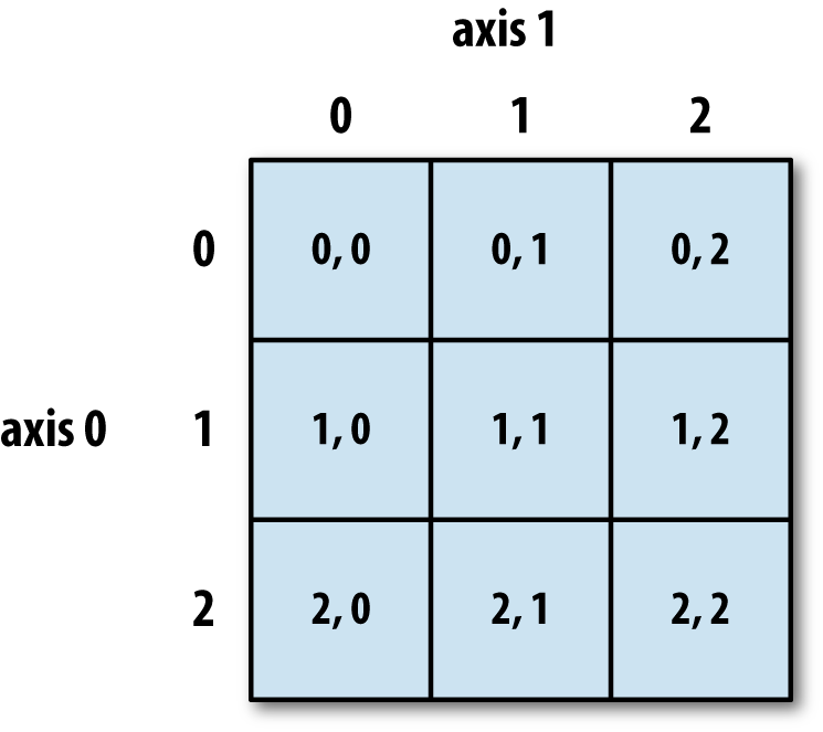
In multidimensional arrays, if you omit later indices, the
returned object will be a lower dimensional ndarray consisting of all
the data along the higher dimensions. So in the 2 × 2 × 3 array arr3d:
In[76]:arr3d=np.array([[[1,2,3],[4,5,6]],[[7,8,9],[10,11,12]]])In[77]:arr3dOut[77]:array([[[1,2,3],[4,5,6]],[[7,8,9],[10,11,12]]])
arr3d[0] is a 2 × 3
array:
In[78]:arr3d[0]Out[78]:array([[1,2,3],[4,5,6]])
Both scalar values and arrays can be assigned to arr3d[0]:
In[79]:old_values=arr3d[0].copy()In[80]:arr3d[0]=42In[81]:arr3dOut[81]:array([[[42,42,42],[42,42,42]],[[7,8,9],[10,11,12]]])In[82]:arr3d[0]=old_valuesIn[83]:arr3dOut[83]:array([[[1,2,3],[4,5,6]],[[7,8,9],[10,11,12]]])
Similarly, arr3d[1, 0] gives
you all of the values whose indices start with (1, 0), forming a 1-dimensional array:
In[84]:arr3d[1,0]Out[84]:array([7,8,9])
This expression is the same as though we had indexed in two steps:
In[85]:x=arr3d[1]In[86]:xOut[86]:array([[7,8,9],[10,11,12]])In[87]:x[0]Out[87]:array([7,8,9])
Note that in all of these cases where subsections of the array have been selected, the returned arrays are views.
Like one-dimensional objects such as Python lists, ndarrays can be sliced with the familiar syntax:
In[88]:arrOut[88]:array([0,1,2,3,4,64,64,64,8,9])In[89]:arr[1:6]Out[89]:array([1,2,3,4,64])
Consider the two-dimensional array from before, arr2d. Slicing this array is a bit
different:
In[90]:arr2dOut[90]:array([[1,2,3],[4,5,6],[7,8,9]])In[91]:arr2d[:2]Out[91]:array([[1,2,3],[4,5,6]])
As you can see, it has sliced along axis 0, the first axis. A
slice, therefore, selects a range of elements along an axis. It can be
helpful to read the expression arr2d[:2] as “select
the first two rows of arr2d.”
You can pass multiple slices just like you can pass multiple indexes:
In[92]:arr2d[:2,1:]Out[92]:array([[2,3],[5,6]])
When slicing like this, you always obtain array views of the same number of dimensions. By mixing integer indexes and slices, you get lower dimensional slices.
For example, I can select the second row but only the first two columns like so:
In[93]:arr2d[1,:2]Out[93]:array([4,5])
Similarly, I can select the third column but only the first two rows like so:
In[94]:arr2d[:2,2]Out[94]:array([3,6])
See Figure 4-2 for an illustration. Note that a colon by itself means to take the entire axis, so you can slice only higher dimensional axes by doing:
In[95]:arr2d[:,:1]Out[95]:array([[1],[4],[7]])
Of course, assigning to a slice expression assigns to the whole selection:
In[96]:arr2d[:2,1:]=0In[97]:arr2dOut[97]:array([[1,0,0],[4,0,0],[7,8,9]])
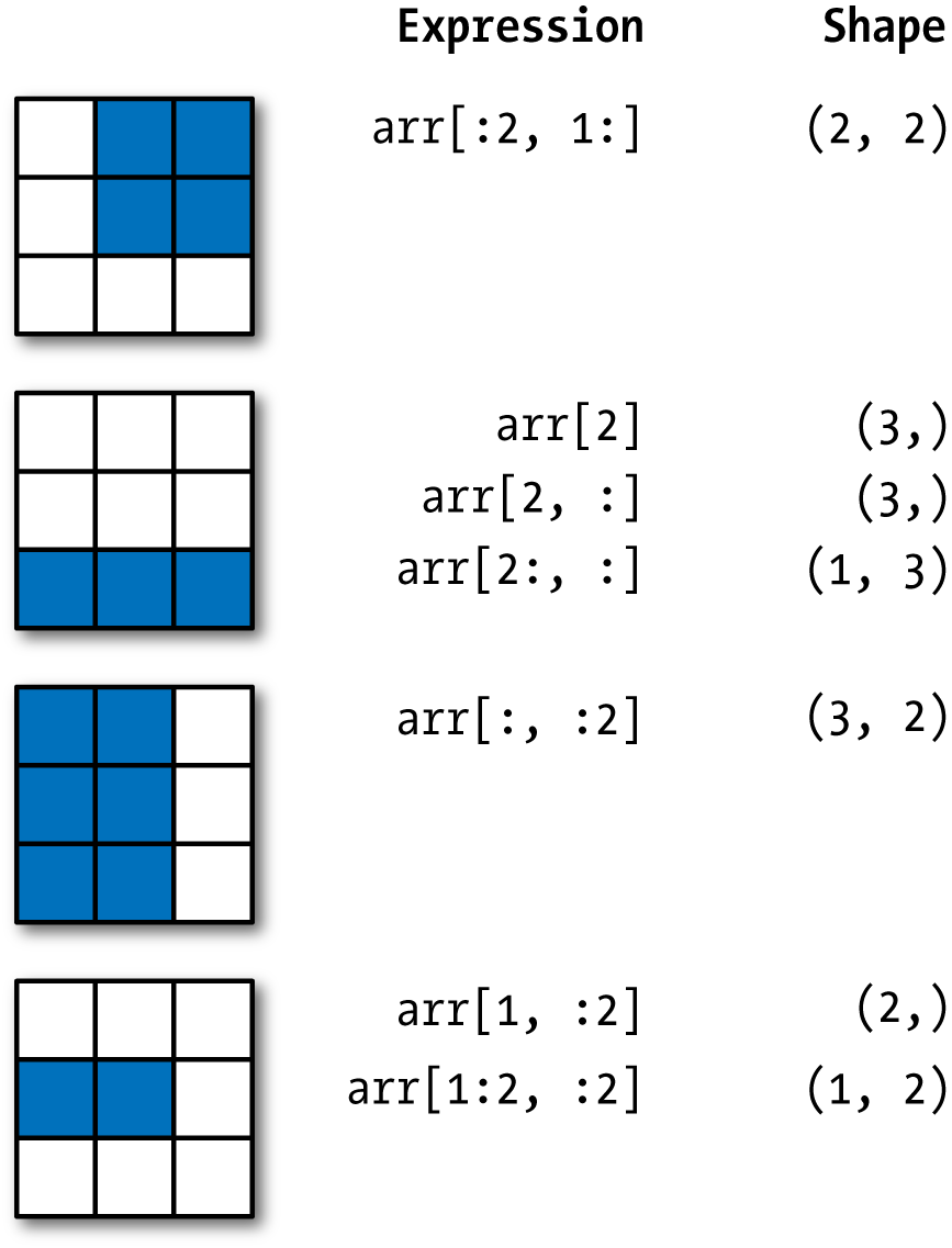
Let’s consider an example where we have some data in an array
and an array of names with duplicates. I’m going to use here the randn function in
numpy.random to generate some random
normally distributed data:
In[98]:names=np.array(['Bob','Joe','Will','Bob','Will','Joe','Joe'])In[99]:data=np.random.randn(7,4)In[100]:namesOut[100]:array(['Bob','Joe','Will','Bob','Will','Joe','Joe'],dtype='<U4')In[101]:dataOut[101]:array([[0.0929,0.2817,0.769,1.2464],[1.0072,-1.2962,0.275,0.2289],[1.3529,0.8864,-2.0016,-0.3718],[1.669,-0.4386,-0.5397,0.477],[3.2489,-1.0212,-0.5771,0.1241],[0.3026,0.5238,0.0009,1.3438],[-0.7135,-0.8312,-2.3702,-1.8608]])
Suppose each name corresponds to a row in the data array and we wanted to select all the
rows with corresponding name 'Bob'.
Like arithmetic operations, comparisons (such as ==) with arrays are also vectorized. Thus,
comparing names with
the string 'Bob' yields a boolean
array:
In[102]:names=='Bob'Out[102]:array([True,False,False,True,False,False,False],dtype=bool)
This boolean array can be passed when indexing the array:
In[103]:data[names=='Bob']Out[103]:array([[0.0929,0.2817,0.769,1.2464],[1.669,-0.4386,-0.5397,0.477]])
The boolean array must be of the same length as the array axis it’s indexing. You can even mix and match boolean arrays with slices or integers (or sequences of integers; more on this later).
Boolean selection will not fail if the boolean array is not the correct length, so I recommend care when using this feature.
In these examples, I select from the rows where names ==
'Bob' and index the columns, too:
In[104]:data[names=='Bob',2:]Out[104]:array([[0.769,1.2464],[-0.5397,0.477]])In[105]:data[names=='Bob',3]Out[105]:array([1.2464,0.477])
To select everything but 'Bob',
you can either use != or negate the
condition using ~:
In[106]:names!='Bob'Out[106]:array([False,True,True,False,True,True,True],dtype=bool)In[107]:data[~(names=='Bob')]Out[107]:array([[1.0072,-1.2962,0.275,0.2289],[1.3529,0.8864,-2.0016,-0.3718],[3.2489,-1.0212,-0.5771,0.1241],[0.3026,0.5238,0.0009,1.3438],[-0.7135,-0.8312,-2.3702,-1.8608]])
The ~ operator can be useful when you want to invert a general
condition:
In[108]:cond=names=='Bob'In[109]:data[~cond]Out[109]:array([[1.0072,-1.2962,0.275,0.2289],[1.3529,0.8864,-2.0016,-0.3718],[3.2489,-1.0212,-0.5771,0.1241],[0.3026,0.5238,0.0009,1.3438],[-0.7135,-0.8312,-2.3702,-1.8608]])
Selecting two of the three names to combine multiple boolean
conditions, use boolean arithmetic operators like & (and) and | (or):
In[110]:mask=(names=='Bob')|(names=='Will')In[111]:maskOut[111]:array([True,False,True,True,True,False,False],dtype=bool)In[112]:data[mask]Out[112]:array([[0.0929,0.2817,0.769,1.2464],[1.3529,0.8864,-2.0016,-0.3718],[1.669,-0.4386,-0.5397,0.477],[3.2489,-1.0212,-0.5771,0.1241]])
Selecting data from an array by boolean indexing always creates a copy of the data, even if the returned array is unchanged.
The Python keywords and and
or do not work with boolean arrays. Use
& (and) and | (or)
instead.
Setting values with boolean arrays works in a common-sense way. To
set all of the negative values in data to 0 we need only do:
In[113]:data[data<0]=0In[114]:dataOut[114]:array([[0.0929,0.2817,0.769,1.2464],[1.0072,0.,0.275,0.2289],[1.3529,0.8864,0.,0.],[1.669,0.,0.,0.477],[3.2489,0.,0.,0.1241],[0.3026,0.5238,0.0009,1.3438],[0.,0.,0.,0.]])
Setting whole rows or columns using a one-dimensional boolean array is also easy:
In[115]:data[names!='Joe']=7In[116]:dataOut[116]:array([[7.,7.,7.,7.],[1.0072,0.,0.275,0.2289],[7.,7.,7.,7.],[7.,7.,7.,7.],[7.,7.,7.,7.],[0.3026,0.5238,0.0009,1.3438],[0.,0.,0.,0.]])
As we will see later, these types of operations on two-dimensional data are convenient to do with pandas.
Fancy indexing is a term adopted by NumPy to describe indexing using integer arrays. Suppose we had an 8 × 4 array:
In[117]:arr=np.empty((8,4))In[118]:foriinrange(8):.....:arr[i]=iIn[119]:arrOut[119]:array([[0.,0.,0.,0.],[1.,1.,1.,1.],[2.,2.,2.,2.],[3.,3.,3.,3.],[4.,4.,4.,4.],[5.,5.,5.,5.],[6.,6.,6.,6.],[7.,7.,7.,7.]])
To select out a subset of the rows in a particular order, you can simply pass a list or ndarray of integers specifying the desired order:
In[120]:arr[[4,3,0,6]]Out[120]:array([[4.,4.,4.,4.],[3.,3.,3.,3.],[0.,0.,0.,0.],[6.,6.,6.,6.]])
Hopefully this code did what you expected! Using negative indices selects rows from the end:
In[121]:arr[[-3,-5,-7]]Out[121]:array([[5.,5.,5.,5.],[3.,3.,3.,3.],[1.,1.,1.,1.]])
Passing multiple index arrays does something slightly different; it selects a one-dimensional array of elements corresponding to each tuple of indices:
In[122]:arr=np.arange(32).reshape((8,4))In[123]:arrOut[123]:array([[0,1,2,3],[4,5,6,7],[8,9,10,11],[12,13,14,15],[16,17,18,19],[20,21,22,23],[24,25,26,27],[28,29,30,31]])In[124]:arr[[1,5,7,2],[0,3,1,2]]Out[124]:array([4,23,29,10])
We’ll look at the reshape method in more detail in
Appendix A.
Here the elements (1, 0), (5, 3), (7,
1), and (2, 2) were
selected. Regardless of how many dimensions the array has (here, only
2), the result of fancy indexing is always one-dimensional.
The behavior of fancy indexing in this case is a bit different from what some users might have expected (myself included), which is the rectangular region formed by selecting a subset of the matrix’s rows and columns. Here is one way to get that:
In[125]:arr[[1,5,7,2]][:,[0,3,1,2]]Out[125]:array([[4,7,5,6],[20,23,21,22],[28,31,29,30],[8,11,9,10]])
Keep in mind that fancy indexing, unlike slicing, always copies the data into a new array.
Transposing is a special form of reshaping that similarly returns a view
on the underlying data without copying anything. Arrays have the transpose method
and also the special T
attribute:
In[126]:arr=np.arange(15).reshape((3,5))In[127]:arrOut[127]:array([[0,1,2,3,4],[5,6,7,8,9],[10,11,12,13,14]])In[128]:arr.TOut[128]:array([[0,5,10],[1,6,11],[2,7,12],[3,8,13],[4,9,14]])
When doing matrix computations, you may do this very often—for
example, when computing the inner matrix product using np.dot:
In[129]:arr=np.random.randn(6,3)In[130]:arrOut[130]:array([[-0.8608,0.5601,-1.2659],[0.1198,-1.0635,0.3329],[-2.3594,-0.1995,-1.542],[-0.9707,-1.307,0.2863],[0.378,-0.7539,0.3313],[1.3497,0.0699,0.2467]])In[131]:np.dot(arr.T,arr)Out[131]:array([[9.2291,0.9394,4.948],[0.9394,3.7662,-1.3622],[4.948,-1.3622,4.3437]])
For higher dimensional arrays, transpose will accept a tuple of axis numbers
to permute the axes (for extra mind bending):
In[132]:arr=np.arange(16).reshape((2,2,4))In[133]:arrOut[133]:array([[[0,1,2,3],[4,5,6,7]],[[8,9,10,11],[12,13,14,15]]])In[134]:arr.transpose((1,0,2))Out[134]:array([[[0,1,2,3],[8,9,10,11]],[[4,5,6,7],[12,13,14,15]]])
Here, the axes have been reordered with the second axis first, the first axis second, and the last axis unchanged.
Simple transposing with .T is a
special case of swapping axes. ndarray has the method swapaxes, which
takes a pair of axis numbers and switches the indicated axes to
rearrange the data:
In[135]:arrOut[135]:array([[[0,1,2,3],[4,5,6,7]],[[8,9,10,11],[12,13,14,15]]])In[136]:arr.swapaxes(1,2)Out[136]:array([[[0,4],[1,5],[2,6],[3,7]],[[8,12],[9,13],[10,14],[11,15]]])
swapaxes similarly returns a
view on the data without making a copy.
A universal function, or ufunc, is a function that performs element-wise operations on data in ndarrays. You can think of them as fast vectorized wrappers for simple functions that take one or more scalar values and produce one or more scalar results.
Many ufuncs are simple element-wise transformations, like sqrt or exp:
In[137]:arr=np.arange(10)In[138]:arrOut[138]:array([0,1,2,3,4,5,6,7,8,9])In[139]:np.sqrt(arr)Out[139]:array([0.,1.,1.4142,1.7321,2.,2.2361,2.4495,2.6458,2.8284,3.])In[140]:np.exp(arr)Out[140]:array([1.,2.7183,7.3891,20.0855,54.5982,148.4132,403.4288,1096.6332,2980.958,8103.0839])
These are referred to as unary ufuncs. Others, such as
add or maximum, take two arrays (thus,
binary ufuncs) and return a single array as the result:
In[141]:x=np.random.randn(8)In[142]:y=np.random.randn(8)In[143]:xOut[143]:array([-0.0119,1.0048,1.3272,-0.9193,-1.5491,0.0222,0.7584,-0.6605])In[144]:yOut[144]:array([0.8626,-0.01,0.05,0.6702,0.853,-0.9559,-0.0235,-2.3042])In[145]:np.maximum(x,y)Out[145]:array([0.8626,1.0048,1.3272,0.6702,0.853,0.0222,0.7584,-0.6605])
Here, numpy.maximum computed the element-wise
maximum of the elements in x and
y.
While not common, a ufunc can return multiple arrays. modf is one example, a vectorized version of the built-in Python
divmod; it returns the fractional and integral parts of a
floating-point array:
In[146]:arr=np.random.randn(7)*5In[147]:arrOut[147]:array([-3.2623,-6.0915,-6.663,5.3731,3.6182,3.45,5.0077])In[148]:remainder,whole_part=np.modf(arr)In[149]:remainderOut[149]:array([-0.2623,-0.0915,-0.663,0.3731,0.6182,0.45,0.0077])In[150]:whole_partOut[150]:array([-3.,-6.,-6.,5.,3.,3.,5.])
Ufuncs accept an optional out argument that
allows them to operate in-place on arrays:
In[151]:arrOut[151]:array([-3.2623,-6.0915,-6.663,5.3731,3.6182,3.45,5.0077])In[152]:np.sqrt(arr)Out[152]:array([nan,nan,nan,2.318,1.9022,1.8574,2.2378])In[153]:np.sqrt(arr,arr)Out[153]:array([nan,nan,nan,2.318,1.9022,1.8574,2.2378])In[154]:arrOut[154]:array([nan,nan,nan,2.318,1.9022,1.8574,2.2378])
See Tables 4-3 and 4-4 for a listing of available ufuncs.
Using NumPy arrays enables you to express many kinds of data processing tasks as concise array expressions that might otherwise require writing loops. This practice of replacing explicit loops with array expressions is commonly referred to as vectorization. In general, vectorized array operations will often be one or two (or more) orders of magnitude faster than their pure Python equivalents, with the biggest impact in any kind of numerical computations. Later, in Appendix A, I explain broadcasting, a powerful method for vectorizing computations.
As a simple example, suppose we wished to evaluate the function
sqrt(x^2 + y^2) across a regular grid
of values. The np.meshgrid function
takes two 1D arrays and produces two 2D matrices
corresponding to all pairs of (x, y) in
the two arrays:
In[155]:points=np.arange(-5,5,0.01)# 1000 equally spaced pointsIn[156]:xs,ys=np.meshgrid(points,points)In[157]:ysOut[157]:array([[-5.,-5.,-5.,...,-5.,-5.,-5.],[-4.99,-4.99,-4.99,...,-4.99,-4.99,-4.99],[-4.98,-4.98,-4.98,...,-4.98,-4.98,-4.98],...,[4.97,4.97,4.97,...,4.97,4.97,4.97],[4.98,4.98,4.98,...,4.98,4.98,4.98],[4.99,4.99,4.99,...,4.99,4.99,4.99]])
Now, evaluating the function is a matter of writing the same expression you would write with two points:
In[158]:z=np.sqrt(xs**2+ys**2)In[159]:zOut[159]:array([[7.0711,7.064,7.0569,...,7.0499,7.0569,7.064],[7.064,7.0569,7.0499,...,7.0428,7.0499,7.0569],[7.0569,7.0499,7.0428,...,7.0357,7.0428,7.0499],...,[7.0499,7.0428,7.0357,...,7.0286,7.0357,7.0428],[7.0569,7.0499,7.0428,...,7.0357,7.0428,7.0499],[7.064,7.0569,7.0499,...,7.0428,7.0499,7.0569]])
As a preview of Chapter 9, I use matplotlib to create visualizations of this two-dimensional array:
In[160]:importmatplotlib.pyplotaspltIn[161]:plt.imshow(z,cmap=plt.cm.gray);plt.colorbar()Out[161]:<matplotlib.colorbar.Colorbarat0x7fa37d95c5f8>In[162]:plt.title("Image plot of $\sqrt{x^2 + y^2}$ for a grid of values")Out[162]:Text(0.5,1,'Image plot of $\\sqrt{x^2 + y^2}$ for a grid of values')
See Figure 4-3. Here I used the
matplotlib function imshow to
create an image plot from a two-dimensional array of
function values.

The numpy.where function is a
vectorized version of the ternary expression x if condition else y. Suppose we had a
boolean array and two arrays of values:
In[165]:xarr=np.array([1.1,1.2,1.3,1.4,1.5])In[166]:yarr=np.array([2.1,2.2,2.3,2.4,2.5])In[167]:cond=np.array([True,False,True,True,False])
Suppose we wanted to take a value from xarr whenever the corresponding value in
cond is True, and otherwise take the value from yarr. A list comprehension doing this might
look like:
In[168]:result=[(xifcelsey).....:forx,y,cinzip(xarr,yarr,cond)]In[169]:resultOut[169]:[1.1000000000000001,2.2000000000000002,1.3,1.3999999999999999,2.5]
This has multiple problems. First, it will not be very fast for
large arrays (because all the work is being done in interpreted Python
code). Second, it will not work with multidimensional arrays. With
np.where you can write this very
concisely:
In[170]:result=np.where(cond,xarr,yarr)In[171]:resultOut[171]:array([1.1,2.2,1.3,1.4,2.5])
The second and third arguments to np.where don’t need to be arrays; one or both
of them can be scalars. A typical use of where in data analysis is to produce a new
array of values based on another array. Suppose you had a matrix of
randomly generated data and you wanted to replace all positive values
with 2 and all negative values with –2. This is very easy to do with
np.where:
In[172]:arr=np.random.randn(4,4)In[173]:arrOut[173]:array([[-0.5031,-0.6223,-0.9212,-0.7262],[0.2229,0.0513,-1.1577,0.8167],[0.4336,1.0107,1.8249,-0.9975],[0.8506,-0.1316,0.9124,0.1882]])In[174]:arr>0Out[174]:array([[False,False,False,False],[True,True,False,True],[True,True,True,False],[True,False,True,True]],dtype=bool)In[175]:np.where(arr>0,2,-2)Out[175]:array([[-2,-2,-2,-2],[2,2,-2,2],[2,2,2,-2],[2,-2,2,2]])
You can combine scalars and arrays when using
np.where. For example, I can replace all positive
values in arr with the constant 2 like so:
In[176]:np.where(arr>0,2,arr)# set only positive values to 2Out[176]:array([[-0.5031,-0.6223,-0.9212,-0.7262],[2.,2.,-1.1577,2.],[2.,2.,2.,-0.9975],[2.,-0.1316,2.,2.]])
The arrays passed to np.where can be more than
just equal-sized arrays or scalars.
A set of mathematical functions that compute statistics about an entire array or about
the data along an axis are accessible as methods of the array class.
You can use aggregations (often called reductions) like sum, mean,
and std (standard deviation) either
by calling the array instance method or using the top-level
NumPy function.
Here I generate some normally distributed random data and compute some aggregate statistics:
In[177]:arr=np.random.randn(5,4)In[178]:arrOut[178]:array([[2.1695,-0.1149,2.0037,0.0296],[0.7953,0.1181,-0.7485,0.585],[0.1527,-1.5657,-0.5625,-0.0327],[-0.929,-0.4826,-0.0363,1.0954],[0.9809,-0.5895,1.5817,-0.5287]])In[179]:arr.mean()Out[179]:0.19607051119998253In[180]:np.mean(arr)Out[180]:0.19607051119998253In[181]:arr.sum()Out[181]:3.9214102239996507
Functions like mean and
sum take an optional axis argument that computes the statistic
over the given axis, resulting in an array with one fewer
dimension:
In[182]:arr.mean(axis=1)Out[182]:array([1.022,0.1875,-0.502,-0.0881,0.3611])In[183]:arr.sum(axis=0)Out[183]:array([3.1693,-2.6345,2.2381,1.1486])
Here, arr.mean(1) means “compute mean across the columns” where
arr.sum(0) means “compute sum down the rows.”
Other methods like cumsum and
cumprod do not aggregate, instead
producing an array of the intermediate results:
In[184]:arr=np.array([0,1,2,3,4,5,6,7])In[185]:arr.cumsum()Out[185]:array([0,1,3,6,10,15,21,28])
In multidimensional arrays, accumulation functions like
cumsum return an array of the same size, but with the
partial aggregates computed along the indicated axis according to each
lower dimensional slice:
In[186]:arr=np.array([[0,1,2],[3,4,5],[6,7,8]])In[187]:arrOut[187]:array([[0,1,2],[3,4,5],[6,7,8]])In[188]:arr.cumsum(axis=0)Out[188]:array([[0,1,2],[3,5,7],[9,12,15]])In[189]:arr.cumprod(axis=1)Out[189]:array([[0,0,0],[3,12,60],[6,42,336]])
See Table 4-5 for a full listing. We’ll see many examples of these methods in action in later chapters.
Boolean values are coerced to 1 (True)
and 0 (False) in the preceding
methods. Thus, sum is often used as a
means of counting True values in a
boolean array:
In[190]:arr=np.random.randn(100)In[191]:(arr>0).sum()# Number of positive valuesOut[191]:42
There are two additional methods, any and
all, useful especially for boolean
arrays. any tests whether one or more
values in an array is True, while
all checks if every value is True:
In[192]:bools=np.array([False,False,True,False])In[193]:bools.any()Out[193]:TrueIn[194]:bools.all()Out[194]:False
These methods also work with non-boolean arrays, where non-zero
elements evaluate to True.
Like Python’s built-in list type, NumPy arrays can be sorted in-place with the sort method:
In[195]:arr=np.random.randn(6)In[196]:arrOut[196]:array([0.6095,-0.4938,1.24,-0.1357,1.43,-0.8469])In[197]:arr.sort()In[198]:arrOut[198]:array([-0.8469,-0.4938,-0.1357,0.6095,1.24,1.43])
You can sort each one-dimensional section of values in a multidimensional array
in-place along an axis by passing the axis number to
sort:
In[199]:arr=np.random.randn(5,3)In[200]:arrOut[200]:array([[0.6033,1.2636,-0.2555],[-0.4457,0.4684,-0.9616],[-1.8245,0.6254,1.0229],[1.1074,0.0909,-0.3501],[0.218,-0.8948,-1.7415]])In[201]:arr.sort(1)In[202]:arrOut[202]:array([[-0.2555,0.6033,1.2636],[-0.9616,-0.4457,0.4684],[-1.8245,0.6254,1.0229],[-0.3501,0.0909,1.1074],[-1.7415,-0.8948,0.218]])
The top-level method np.sort
returns a sorted copy of an array instead of modifying the array
in-place. A quick-and-dirty way to compute the quantiles of an array is
to sort it and select the value at a particular rank:
In[203]:large_arr=np.random.randn(1000)In[204]:large_arr.sort()In[205]:large_arr[int(0.05*len(large_arr))]# 5% quantileOut[205]:-1.5311513550102103
For more details on using NumPy’s sorting methods, and more advanced techniques like indirect sorts, see Appendix A. Several other kinds of data manipulations related to sorting (e.g., sorting a table of data by one or more columns) can also be found in pandas.
NumPy has some basic set operations for one-dimensional ndarrays. A commonly
used one is np.unique, which
returns the sorted unique values in an array:
In[206]:names=np.array(['Bob','Joe','Will','Bob','Will','Joe','Joe'])In[207]:np.unique(names)Out[207]:array(['Bob','Joe','Will'],dtype='<U4')In[208]:ints=np.array([3,3,3,2,2,1,1,4,4])In[209]:np.unique(ints)Out[209]:array([1,2,3,4])
Contrast np.unique with the
pure Python alternative:
In[210]:sorted(set(names))Out[210]:['Bob','Joe','Will']
Another function, np.in1d,
tests membership of the values in one array in another,
returning a boolean array:
In[211]:values=np.array([6,0,0,3,2,5,6])In[212]:np.in1d(values,[2,3,6])Out[212]:array([True,False,False,True,True,False,True],dtype=bool)
See Table 4-6 for a listing of set functions in NumPy.
NumPy is able to save and load data to and from disk either in text or binary format. In this section I only discuss NumPy’s built-in binary format, since most users will prefer pandas and other tools for loading text or tabular data (see Chapter 6 for much more).
np.save and np.load are the two workhorse functions for efficiently saving and
loading array data on disk. Arrays are saved by default in an uncompressed
raw binary format with file extension .npy:
In[213]:arr=np.arange(10)In[214]:np.save('some_array',arr)
If the file path does not already end in .npy,
the extension will be appended. The array on disk can then be loaded with
np.load:
In[215]:np.load('some_array.npy')Out[215]:array([0,1,2,3,4,5,6,7,8,9])
You save multiple arrays in an uncompressed archive using np.savez and
passing the arrays as keyword arguments:
In[216]:np.savez('array_archive.npz',a=arr,b=arr)
When loading an .npz file, you get back a dict-like object that loads the individual arrays lazily:
In[217]:arch=np.load('array_archive.npz')In[218]:arch['b']Out[218]:array([0,1,2,3,4,5,6,7,8,9])
If your data compresses well, you may wish to use numpy.savez_compressed
instead:
In[219]:np.savez_compressed('arrays_compressed.npz',a=arr,b=arr)
Linear algebra, like matrix multiplication, decompositions, determinants,
and other square matrix math, is an important part of any array library.
Unlike some languages like MATLAB, multiplying two two-dimensional arrays
with * is an element-wise product
instead of a matrix dot product. Thus, there is a function dot, both an array method and a function in the numpy namespace, for matrix multiplication:
In[223]:x=np.array([[1.,2.,3.],[4.,5.,6.]])In[224]:y=np.array([[6.,23.],[-1,7],[8,9]])In[225]:xOut[225]:array([[1.,2.,3.],[4.,5.,6.]])In[226]:yOut[226]:array([[6.,23.],[-1.,7.],[8.,9.]])In[227]:x.dot(y)Out[227]:array([[28.,64.],[67.,181.]])
x.dot(y) is equivalent to np.dot(x,
y):
In[228]:np.dot(x,y)Out[228]:array([[28.,64.],[67.,181.]])
A matrix product between a two-dimensional array and a suitably sized one-dimensional array results in a one-dimensional array:
In[229]:np.dot(x,np.ones(3))Out[229]:array([6.,15.])
The @ symbol (as of Python 3.5) also works as an infix operator that
performs matrix multiplication:
In[230]:x@np.ones(3)Out[230]:array([6.,15.])
numpy.linalg has a standard set
of matrix decompositions and things like inverse and determinant. These
are implemented under the hood via the same industry-standard linear
algebra libraries used in other languages like MATLAB and R, such as BLAS,
LAPACK, or possibly (depending on your NumPy build) the proprietary
Intel MKL (Math Kernel Library):
In[231]:fromnumpy.linalgimportinv,qrIn[232]:X=np.random.randn(5,5)In[233]:mat=X.T.dot(X)In[234]:inv(mat)Out[234]:array([[933.1189,871.8258,-1417.6902,-1460.4005,1782.1391],[871.8258,815.3929,-1325.9965,-1365.9242,1666.9347],[-1417.6902,-1325.9965,2158.4424,2222.0191,-2711.6822],[-1460.4005,-1365.9242,2222.0191,2289.0575,-2793.422],[1782.1391,1666.9347,-2711.6822,-2793.422,3409.5128]])In[235]:mat.dot(inv(mat))Out[235]:array([[1.,0.,-0.,-0.,-0.],[-0.,1.,0.,0.,0.],[0.,0.,1.,0.,0.],[-0.,0.,0.,1.,-0.],[-0.,0.,0.,0.,1.]])In[236]:q,r=qr(mat)In[237]:rOut[237]:array([[-1.6914,4.38,0.1757,0.4075,-0.7838],[0.,-2.6436,0.1939,-3.072,-1.0702],[0.,0.,-0.8138,1.5414,0.6155],[0.,0.,0.,-2.6445,-2.1669],[0.,0.,0.,0.,0.0002]])
The expression X.T.dot(X) computes the dot
product of X with its transpose
X.T.
See Table 4-7 for a list of some of the most commonly used linear algebra functions.
The numpy.random module
supplements the built-in Python random with functions for efficiently generating
whole arrays of sample values from many kinds of probability
distributions. For example, you can get a 4 × 4 array of samples from the
standard normal distribution using normal:
In[238]:samples=np.random.normal(size=(4,4))In[239]:samplesOut[239]:array([[0.5732,0.1933,0.4429,1.2796],[0.575,0.4339,-0.7658,-1.237],[-0.5367,1.8545,-0.92,-0.1082],[0.1525,0.9435,-1.0953,-0.144]])
Python’s built-in random module,
by contrast, only samples one value at a time. As you can see from this
benchmark, numpy.random is well over an
order of magnitude faster for generating very large samples:
In[240]:fromrandomimportnormalvariateIn[241]:N=1000000In[242]:%timeitsamples=[normalvariate(0,1)for_inrange(N)]1.54s+-81.9msperloop(mean+-std.dev.of7runs,1loopeach)In[243]:%timeitnp.random.normal(size=N)71.4ms+-8.53msperloop(mean+-std.dev.of7runs,10loopseach)
We say that these are pseudorandom numbers
because they are generated by an algorithm with deterministic behavior
based on the seed of the random number generator. You
can change NumPy’s random number generation seed using
np.random.seed:
In[244]:np.random.seed(1234)
The data generation functions in numpy.random use
a global random seed. To avoid global state, you can use
numpy.random.RandomState to create a random number generator isolated from
others:
In[245]:rng=np.random.RandomState(1234)In[246]:rng.randn(10)Out[246]:array([0.4714,-1.191,1.4327,-0.3127,-0.7206,0.8872,0.8596,-0.6365,0.0157,-2.2427])
See Table 4-8 for a partial list of
functions available in numpy.random.
I’ll give some examples of leveraging these functions’ ability to generate
large arrays of samples all at once in the next section.
The simulation of random walks provides an illustrative application of utilizing array operations. Let’s first consider a simple random walk starting at 0 with steps of 1 and –1 occurring with equal probability.
Here is a pure Python way to implement a single random walk with
1,000 steps using the built-in random
module:
In[247]:importrandom.....:position=0.....:walk=[position].....:steps=1000.....:foriinrange(steps):.....:step=1ifrandom.randint(0,1)else-1.....:position+=step.....:walk.append(position).....:
See Figure 4-4 for an example plot of the first 100 values on one of these random walks:
In[249]:plt.plot(walk[:100])
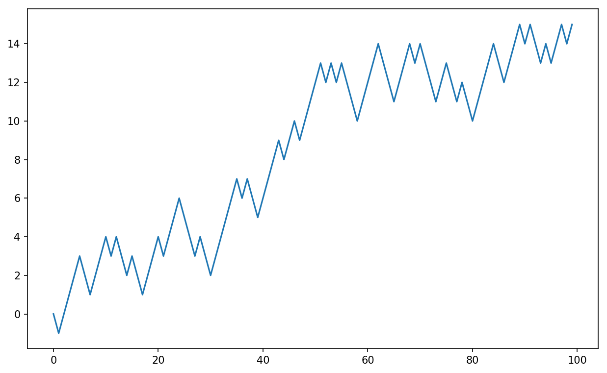
You might make the observation that walk is simply the cumulative sum of the random
steps and could be evaluated as an array expression. Thus, I use the
np.random module to draw 1,000 coin
flips at once, set these to 1 and –1, and compute the cumulative
sum:
In[251]:nsteps=1000In[252]:draws=np.random.randint(0,2,size=nsteps)In[253]:steps=np.where(draws>0,1,-1)In[254]:walk=steps.cumsum()
From this we can begin to extract statistics like the minimum and maximum value along the walk’s trajectory:
In[255]:walk.min()Out[255]:-3In[256]:walk.max()Out[256]:31
A more complicated statistic is the first crossing
time, the step at which the random walk reaches a particular
value. Here we might want to know how long it took the random walk to get
at least 10 steps away from the origin 0 in either direction. np.abs(walk) >=
10 gives us a boolean array indicating where the walk has
reached or exceeded 10, but we want the index of the
first 10 or –10. Turns out, we can compute this
using argmax, which
returns the first index of the maximum value in the boolean array
(True is the maximum value):
In[257]:(np.abs(walk)>=10).argmax()Out[257]:37
Note that using argmax here is
not always efficient because it always makes a full scan of the array. In
this special case, once a True is
observed we know it to be the maximum value.
If your goal was to simulate many random walks, say 5,000 of them,
you can generate all of the random walks with minor modifications to the
preceding code. If passed a 2-tuple, the numpy.random functions will generate a
two-dimensional array of draws, and we can compute the cumulative sum
across the rows to compute all 5,000 random walks in one shot:
In[258]:nwalks=5000In[259]:nsteps=1000In[260]:draws=np.random.randint(0,2,size=(nwalks,nsteps))# 0 or 1In[261]:steps=np.where(draws>0,1,-1)In[262]:walks=steps.cumsum(1)In[263]:walksOut[263]:array([[1,0,1,...,8,7,8],[1,0,-1,...,34,33,32],[1,0,-1,...,4,5,4],...,[1,2,1,...,24,25,26],[1,2,3,...,14,13,14],[-1,-2,-3,...,-24,-23,-22]])
Now, we can compute the maximum and minimum values obtained over all of the walks:
In[264]:walks.max()Out[264]:138In[265]:walks.min()Out[265]:-133
Out of these walks, let’s compute the minimum crossing time to 30
or –30. This is slightly tricky because not all 5,000 of them reach 30.
We can check this using the any method:
In[266]:hits30=(np.abs(walks)>=30).any(1)In[267]:hits30Out[267]:array([False,True,False,...,False,True,False],dtype=bool)In[268]:hits30.sum()# Number that hit 30 or -30Out[268]:3410
We can use this boolean array to select out the rows of walks that actually cross the absolute 30
level and call argmax across axis 1
to get the crossing times:
In[269]:crossing_times=(np.abs(walks[hits30])>=30).argmax(1)In[270]:crossing_times.mean()Out[270]:498.88973607038122
Feel free to experiment with other distributions for the steps
other than equal-sized coin flips. You need only use a different random
number generation function, like normal to generate normally distributed steps
with some mean and standard deviation:
In[271]:steps=np.random.normal(loc=0,scale=0.25,.....:size=(nwalks,nsteps))
While much of the rest of the book will focus on building data wrangling skills with pandas, we will continue to work in a similar array-based style. In Appendix A, we will dig deeper into NumPy features to help you further develop your array computing skills.
pandas will be a major tool of interest throughout much of the rest of the
book. It contains data structures and data manipulation tools designed to
make data cleaning and analysis fast and easy in Python. pandas is often
used in tandem with numerical computing tools like NumPy and SciPy,
analytical libraries like statsmodels and scikit-learn, and data
visualization libraries like matplotlib. pandas adopts significant parts of
NumPy’s idiomatic style of array-based computing, especially array-based
functions and a preference for data processing without
for loops.
While pandas adopts many coding idioms from NumPy, the biggest difference is that pandas is designed for working with tabular or heterogeneous data. NumPy, by contrast, is best suited for working with homogeneous numerical array data.
Since becoming an open source project in 2010, pandas has matured into a quite large library that’s applicable in a broad set of real-world use cases. The developer community has grown to over 800 distinct contributors, who’ve been helping build the project as they’ve used it to solve their day-to-day data problems.
Throughout the rest of the book, I use the following import convention for pandas:
In[1]:importpandasaspd
Thus, whenever you see pd. in code,
it’s referring to pandas. You may also find it easier to import Series and
DataFrame into the local namespace since they are so frequently used:
In[2]:frompandasimportSeries,DataFrame
To get started with pandas, you will need to get comfortable with its two workhorse data structures: Series and DataFrame. While they are not a universal solution for every problem, they provide a solid, easy-to-use basis for most applications.
A Series is a one-dimensional array-like object containing a sequence of values (of similar types to NumPy types) and an associated array of data labels, called its index. The simplest Series is formed from only an array of data:
In[11]:obj=pd.Series([4,7,-5,3])In[12]:objOut[12]:04172-533dtype:int64
The string representation of a Series displayed interactively
shows the index on the left and the values on the right. Since we did
not specify an index for the data, a default one consisting of the
integers 0 through N - 1 (where
N is the length of the data) is created. You can get
the array representation and index object of the Series via its values
and index attributes, respectively:
In[13]:obj.valuesOut[13]:array([4,7,-5,3])In[14]:obj.index# like range(4)Out[14]:RangeIndex(start=0,stop=4,step=1)
Often it will be desirable to create a Series with an index identifying each data point with a label:
In[15]:obj2=pd.Series([4,7,-5,3],index=['d','b','a','c'])In[16]:obj2Out[16]:d4b7a-5c3dtype:int64In[17]:obj2.indexOut[17]:Index(['d','b','a','c'],dtype='object')
Compared with NumPy arrays, you can use labels in the index when selecting single values or a set of values:
In[18]:obj2['a']Out[18]:-5In[19]:obj2['d']=6In[20]:obj2[['c','a','d']]Out[20]:c3a-5d6dtype:int64
Here ['c', 'a', 'd'] is interpreted as a list
of indices, even though it contains strings instead of integers.
Using NumPy functions or NumPy-like operations, such as filtering with a boolean array, scalar multiplication, or applying math functions, will preserve the index-value link:
In[21]:obj2[obj2>0]Out[21]:d6b7c3dtype:int64In[22]:obj2*2Out[22]:d12b14a-10c6dtype:int64In[23]:np.exp(obj2)Out[23]:d403.428793b1096.633158a0.006738c20.085537dtype:float64
Another way to think about a Series is as a fixed-length, ordered dict, as it is a mapping of index values to data values. It can be used in many contexts where you might use a dict:
In[24]:'b'inobj2Out[24]:TrueIn[25]:'e'inobj2Out[25]:False
Should you have data contained in a Python dict, you can create a Series from it by passing the dict:
In[26]:sdata={'Ohio':35000,'Texas':71000,'Oregon':16000,'Utah':5000}In[27]:obj3=pd.Series(sdata)In[28]:obj3Out[28]:Ohio35000Oregon16000Texas71000Utah5000dtype:int64
When you are only passing a dict, the index in the resulting Series will have the dict’s keys in sorted order. You can override this by passing the dict keys in the order you want them to appear in the resulting Series:
In[29]:states=['California','Ohio','Oregon','Texas']In[30]:obj4=pd.Series(sdata,index=states)In[31]:obj4Out[31]:CaliforniaNaNOhio35000.0Oregon16000.0Texas71000.0dtype:float64
Here, three values found in sdata were placed in the appropriate
locations, but since no value for 'California' was found, it appears as NaN (not a number),
which is considered in pandas to mark missing or NA
values. Since 'Utah' was not included in
states, it is excluded from the resulting
object.
I will use the terms “missing” or “NA” interchangeably to refer to
missing data. The isnull and notnull functions
in pandas should be used to detect missing data:
In[32]:pd.isnull(obj4)Out[32]:CaliforniaTrueOhioFalseOregonFalseTexasFalsedtype:boolIn[33]:pd.notnull(obj4)Out[33]:CaliforniaFalseOhioTrueOregonTrueTexasTruedtype:bool
Series also has these as instance methods:
In[34]:obj4.isnull()Out[34]:CaliforniaTrueOhioFalseOregonFalseTexasFalsedtype:bool
I discuss working with missing data in more detail in Chapter 7.
A useful Series feature for many applications is that it automatically aligns by index label in arithmetic operations:
In[35]:obj3Out[35]:Ohio35000Oregon16000Texas71000Utah5000dtype:int64In[36]:obj4Out[36]:CaliforniaNaNOhio35000.0Oregon16000.0Texas71000.0dtype:float64In[37]:obj3+obj4Out[37]:CaliforniaNaNOhio70000.0Oregon32000.0Texas142000.0UtahNaNdtype:float64
Data alignment features will be addressed in more detail later. If you have experience with databases, you can think about this as being similar to a join operation.
Both the Series object itself and its index have a name attribute, which
integrates with other key areas of pandas functionality:
In[38]:obj4.name='population'In[39]:obj4.index.name='state'In[40]:obj4Out[40]:stateCaliforniaNaNOhio35000.0Oregon16000.0Texas71000.0Name:population,dtype:float64
A Series’s index can be altered in-place by assignment:
In[41]:objOut[41]:04172-533dtype:int64In[42]:obj.index=['Bob','Steve','Jeff','Ryan']In[43]:objOut[43]:Bob4Steve7Jeff-5Ryan3dtype:int64
A DataFrame represents a rectangular table of data and contains an ordered collection of columns, each of which can be a different value type (numeric, string, boolean, etc.). The DataFrame has both a row and column index; it can be thought of as a dict of Series all sharing the same index. Under the hood, the data is stored as one or more two-dimensional blocks rather than a list, dict, or some other collection of one-dimensional arrays. The exact details of DataFrame’s internals are outside the scope of this book.
While a DataFrame is physically two-dimensional, you can use it to represent higher dimensional data in a tabular format using hierarchical indexing, a subject we will discuss in Chapter 8 and an ingredient in some of the more advanced data-handling features in pandas.
There are many ways to construct a DataFrame, though one of the most common is from a dict of equal-length lists or NumPy arrays:
data={'state':['Ohio','Ohio','Ohio','Nevada','Nevada','Nevada'],'year':[2000,2001,2002,2001,2002,2003],'pop':[1.5,1.7,3.6,2.4,2.9,3.2]}frame=pd.DataFrame(data)
The resulting DataFrame will have its index assigned automatically as with Series, and the columns are placed in sorted order:
In[45]:frameOut[45]:popstateyear01.5Ohio200011.7Ohio200123.6Ohio200232.4Nevada200142.9Nevada200253.2Nevada2003
If you are using the Jupyter notebook, pandas DataFrame objects will be displayed as a more browser-friendly HTML table.
For large DataFrames, the head method
selects only the first five rows:
In[46]:frame.head()Out[46]:popstateyear01.5Ohio200011.7Ohio200123.6Ohio200232.4Nevada200142.9Nevada2002
If you specify a sequence of columns, the DataFrame’s columns will be arranged in that order:
In[47]:pd.DataFrame(data,columns=['year','state','pop'])Out[47]:yearstatepop02000Ohio1.512001Ohio1.722002Ohio3.632001Nevada2.442002Nevada2.952003Nevada3.2
If you pass a column that isn’t contained in the dict, it will appear with missing values in the result:
In[48]:frame2=pd.DataFrame(data,columns=['year','state','pop','debt'],....:index=['one','two','three','four',....:'five','six'])In[49]:frame2Out[49]:yearstatepopdebtone2000Ohio1.5NaNtwo2001Ohio1.7NaNthree2002Ohio3.6NaNfour2001Nevada2.4NaNfive2002Nevada2.9NaNsix2003Nevada3.2NaNIn[50]:frame2.columnsOut[50]:Index(['year','state','pop','debt'],dtype='object')
A column in a DataFrame can be retrieved as a Series either by dict-like notation or by attribute:
In[51]:frame2['state']Out[51]:oneOhiotwoOhiothreeOhiofourNevadafiveNevadasixNevadaName:state,dtype:objectIn[52]:frame2.yearOut[52]:one2000two2001three2002four2001five2002six2003Name:year,dtype:int64
Attribute-like access (e.g., frame2.year) and
tab completion of column names in IPython is provided as a
convenience.
frame2[column] works for any column name, but
frame2.column only works when the column name is a
valid Python variable name.
Note that the returned Series have the same index as the
DataFrame, and their name attribute has been
appropriately set.
Rows can also be retrieved by position or name with the
special loc attribute
(much more on this later):
In[53]:frame2.loc['three']Out[53]:year2002stateOhiopop3.6debtNaNName:three,dtype:object
Columns can be modified by assignment. For example, the empty
'debt' column could be assigned a
scalar value or an array of values:
In[54]:frame2['debt']=16.5In[55]:frame2Out[55]:yearstatepopdebtone2000Ohio1.516.5two2001Ohio1.716.5three2002Ohio3.616.5four2001Nevada2.416.5five2002Nevada2.916.5six2003Nevada3.216.5In[56]:frame2['debt']=np.arange(6.)In[57]:frame2Out[57]:yearstatepopdebtone2000Ohio1.50.0two2001Ohio1.71.0three2002Ohio3.62.0four2001Nevada2.43.0five2002Nevada2.94.0six2003Nevada3.25.0
When you are assigning lists or arrays to a column, the value’s length must match the length of the DataFrame. If you assign a Series, its labels will be realigned exactly to the DataFrame’s index, inserting missing values in any holes:
In[58]:val=pd.Series([-1.2,-1.5,-1.7],index=['two','four','five'])In[59]:frame2['debt']=valIn[60]:frame2Out[60]:yearstatepopdebtone2000Ohio1.5NaNtwo2001Ohio1.7-1.2three2002Ohio3.6NaNfour2001Nevada2.4-1.5five2002Nevada2.9-1.7six2003Nevada3.2NaN
Assigning a column that doesn’t exist will create a new column.
The del keyword will delete columns as with a dict.
As an example of del, I first add a new column
of boolean values where the state column equals
'Ohio':
In[61]:frame2['eastern']=frame2.state=='Ohio'In[62]:frame2Out[62]:yearstatepopdebteasternone2000Ohio1.5NaNTruetwo2001Ohio1.7-1.2Truethree2002Ohio3.6NaNTruefour2001Nevada2.4-1.5Falsefive2002Nevada2.9-1.7Falsesix2003Nevada3.2NaNFalse
New columns cannot be created with the
frame2.eastern syntax.
The del method can then be used to remove this column:
In[63]:delframe2['eastern']In[64]:frame2.columnsOut[64]:Index(['year','state','pop','debt'],dtype='object')
The column returned from indexing a DataFrame is a
view on the underlying data, not a copy. Thus,
any in-place modifications to the Series will be reflected in the
DataFrame. The column can be explicitly copied with the Series’s copy
method.
Another common form of data is a nested dict of dicts:
In[65]:pop={'Nevada':{2001:2.4,2002:2.9},....:'Ohio':{2000:1.5,2001:1.7,2002:3.6}}
If the nested dict is passed to the DataFrame, pandas will interpret the outer dict keys as the columns and the inner keys as the row indices:
In[66]:frame3=pd.DataFrame(pop)In[67]:frame3Out[67]:NevadaOhio2000NaN1.520012.41.720022.93.6
You can transpose the DataFrame (swap rows and columns) with similar syntax to a NumPy array:
In[68]:frame3.TOut[68]:200020012002NevadaNaN2.42.9Ohio1.51.73.6
The keys in the inner dicts are combined and sorted to form the index in the result. This isn’t true if an explicit index is specified:
In[69]:pd.DataFrame(pop,index=[2001,2002,2003])Out[69]:NevadaOhio20012.41.720022.93.62003NaNNaN
Dicts of Series are treated in much the same way:
In[70]:pdata={'Ohio':frame3['Ohio'][:-1],....:'Nevada':frame3['Nevada'][:2]}In[71]:pd.DataFrame(pdata)Out[71]:NevadaOhio2000NaN1.520012.41.7
For a complete list of things you can pass the DataFrame constructor, see Table 5-1.
If a DataFrame’s index and
columns have their name attributes set, these will also be
displayed:
In[72]:frame3.index.name='year';frame3.columns.name='state'In[73]:frame3Out[73]:stateNevadaOhioyear2000NaN1.520012.41.720022.93.6
As with Series, the values
attribute returns the data contained in the DataFrame as a
two-dimensional ndarray:
In[74]:frame3.valuesOut[74]:array([[nan,1.5],[2.4,1.7],[2.9,3.6]])
If the DataFrame’s columns are different dtypes, the dtype of the values array will be chosen to accommodate all of the columns:
In[75]:frame2.valuesOut[75]:array([[2000,'Ohio',1.5,nan],[2001,'Ohio',1.7,-1.2],[2002,'Ohio',3.6,nan],[2001,'Nevada',2.4,-1.5],[2002,'Nevada',2.9,-1.7],[2003,'Nevada',3.2,nan]],dtype=object)
pandas’s Index objects are responsible for holding the axis labels and other metadata (like the axis name or names). Any array or other sequence of labels you use when constructing a Series or DataFrame is internally converted to an Index:
In[76]:obj=pd.Series(range(3),index=['a','b','c'])In[77]:index=obj.indexIn[78]:indexOut[78]:Index(['a','b','c'],dtype='object')In[79]:index[1:]Out[79]:Index(['b','c'],dtype='object')
Index objects are immutable and thus can’t be modified by the user:
index[1]='d'# TypeError
Immutability makes it safer to share Index objects among data structures:
In[80]:labels=pd.Index(np.arange(3))In[81]:labelsOut[81]:Int64Index([0,1,2],dtype='int64')In[82]:obj2=pd.Series([1.5,-2.5,0],index=labels)In[83]:obj2Out[83]:01.51-2.520.0dtype:float64In[84]:obj2.indexislabelsOut[84]:True
Some users will not often take advantage of the capabilities provided by indexes, but because some operations will yield results containing indexed data, it’s important to understand how they work.
In addition to being array-like, an Index also behaves like a fixed-size set:
In[85]:frame3Out[85]:stateNevadaOhioyear2000NaN1.520012.41.720022.93.6In[86]:frame3.columnsOut[86]:Index(['Nevada','Ohio'],dtype='object',name='state')In[87]:'Ohio'inframe3.columnsOut[87]:TrueIn[88]:2003inframe3.indexOut[88]:False
Unlike Python sets, a pandas Index can contain duplicate labels:
In[89]:dup_labels=pd.Index(['foo','foo','bar','bar'])In[90]:dup_labelsOut[90]:Index(['foo','foo','bar','bar'],dtype='object')
Selections with duplicate labels will select all occurrences of that label.
Each Index has a number of methods and properties for set logic, which answer other common questions about the data it contains. Some useful ones are summarized in Table 5-2.
This section will walk you through the fundamental mechanics of interacting with the data contained in a Series or DataFrame. In the chapters to come, we will delve more deeply into data analysis and manipulation topics using pandas. This book is not intended to serve as exhaustive documentation for the pandas library; instead, we’ll focus on the most important features, leaving the less common (i.e., more esoteric) things for you to explore on your own.
An important method on pandas objects is reindex, which means to create a new object
with the data conformed to a new index. Consider an
example:
In[91]:obj=pd.Series([4.5,7.2,-5.3,3.6],index=['d','b','a','c'])In[92]:objOut[92]:d4.5b7.2a-5.3c3.6dtype:float64
Calling reindex on this Series
rearranges the data according to the new index, introducing missing
values if any index values were not already present:
In[93]:obj2=obj.reindex(['a','b','c','d','e'])In[94]:obj2Out[94]:a-5.3b7.2c3.6d4.5eNaNdtype:float64
For ordered data like time series, it may be desirable to do some
interpolation or filling of values when reindexing. The method option allows us to do this, using a
method such as ffill, which forward-fills the values:
In[95]:obj3=pd.Series(['blue','purple','yellow'],index=[0,2,4])In[96]:obj3Out[96]:0blue2purple4yellowdtype:objectIn[97]:obj3.reindex(range(6),method='ffill')Out[97]:0blue1blue2purple3purple4yellow5yellowdtype:object
With DataFrame, reindex can
alter either the (row) index, columns, or both. When passed only a
sequence, it reindexes the rows in the result:
In[98]:frame=pd.DataFrame(np.arange(9).reshape((3,3)),....:index=['a','c','d'],....:columns=['Ohio','Texas','California'])In[99]:frameOut[99]:OhioTexasCaliforniaa012c345d678In[100]:frame2=frame.reindex(['a','b','c','d'])In[101]:frame2Out[101]:OhioTexasCaliforniaa0.01.02.0bNaNNaNNaNc3.04.05.0d6.07.08.0
The columns can be reindexed with the columns keyword:
In[102]:states=['Texas','Utah','California']In[103]:frame.reindex(columns=states)Out[103]:TexasUtahCaliforniaa1NaN2c4NaN5d7NaN8
See Table 5-3 for more about the
arguments to reindex.
As we’ll explore in more detail, you can reindex more
succinctly by label-indexing with loc, and many users prefer to use it
exclusively:
In[104]:frame.loc[['a','b','c','d'],states]Out[104]:TexasUtahCaliforniaa1.0NaN2.0bNaNNaNNaNc4.0NaN5.0d7.0NaN8.0
Dropping one or more entries from an axis is easy if you already have an index
array or list without those entries. As that can require a bit of
munging and set logic, the drop method will
return a new object with the indicated value or values deleted from an
axis:
In[105]:obj=pd.Series(np.arange(5.),index=['a','b','c','d','e'])In[106]:objOut[106]:a0.0b1.0c2.0d3.0e4.0dtype:float64In[107]:new_obj=obj.drop('c')In[108]:new_objOut[108]:a0.0b1.0d3.0e4.0dtype:float64In[109]:obj.drop(['d','c'])Out[109]:a0.0b1.0e4.0dtype:float64
With DataFrame, index values can be deleted from either axis. To illustrate this, we first create an example DataFrame:
In[110]:data=pd.DataFrame(np.arange(16).reshape((4,4)),.....:index=['Ohio','Colorado','Utah','New York'],.....:columns=['one','two','three','four'])In[111]:dataOut[111]:onetwothreefourOhio0123Colorado4567Utah891011NewYork12131415
Calling drop with a sequence of labels will
drop values from the row labels (axis 0):
In[112]:data.drop(['Colorado','Ohio'])Out[112]:onetwothreefourUtah891011NewYork12131415
You can drop values from the columns by passing
axis=1 or axis='columns':
In[113]:data.drop('two',axis=1)Out[113]:onethreefourOhio023Colorado467Utah81011NewYork121415In[114]:data.drop(['two','four'],axis='columns')Out[114]:onethreeOhio02Colorado46Utah810NewYork1214
Many functions, like drop, which modify the
size or shape of a Series or DataFrame, can manipulate an object
in-place without returning a new object:
In[115]:obj.drop('c',inplace=True)In[116]:objOut[116]:a0.0b1.0d3.0e4.0dtype:float64
Be careful with the inplace, as it destroys any
data that is dropped.
Series indexing (obj[...])
works analogously to NumPy array indexing, except you can use
the Series’s index values instead of only integers. Here are some
examples of this:
In[117]:obj=pd.Series(np.arange(4.),index=['a','b','c','d'])In[118]:objOut[118]:a0.0b1.0c2.0d3.0dtype:float64In[119]:obj['b']Out[119]:1.0In[120]:obj[1]Out[120]:1.0In[121]:obj[2:4]Out[121]:c2.0d3.0dtype:float64In[122]:obj[['b','a','d']]Out[122]:b1.0a0.0d3.0dtype:float64In[123]:obj[[1,3]]Out[123]:b1.0d3.0dtype:float64In[124]:obj[obj<2]Out[124]:a0.0b1.0dtype:float64
Slicing with labels behaves differently than normal Python slicing in that the endpoint is inclusive:
In[125]:obj['b':'c']Out[125]:b1.0c2.0dtype:float64
Setting using these methods modifies the corresponding section of the Series:
In[126]:obj['b':'c']=5In[127]:objOut[127]:a0.0b5.0c5.0d3.0dtype:float64
Indexing into a DataFrame is for retrieving one or more columns either with a single value or sequence:
In[128]:data=pd.DataFrame(np.arange(16).reshape((4,4)),.....:index=['Ohio','Colorado','Utah','New York'],.....:columns=['one','two','three','four'])In[129]:dataOut[129]:onetwothreefourOhio0123Colorado4567Utah891011NewYork12131415In[130]:data['two']Out[130]:Ohio1Colorado5Utah9NewYork13Name:two,dtype:int64In[131]:data[['three','one']]Out[131]:threeoneOhio20Colorado64Utah108NewYork1412
Indexing like this has a few special cases. First, slicing or selecting data with a boolean array:
In[132]:data[:2]Out[132]:onetwothreefourOhio0123Colorado4567In[133]:data[data['three']>5]Out[133]:onetwothreefourColorado4567Utah891011NewYork12131415
The row selection syntax data[:2] is provided
as a convenience. Passing a single element or a list to the
[] operator selects columns.
Another use case is in indexing with a boolean DataFrame, such as one produced by a scalar comparison:
In[134]:data<5Out[134]:onetwothreefourOhioTrueTrueTrueTrueColoradoTrueFalseFalseFalseUtahFalseFalseFalseFalseNewYorkFalseFalseFalseFalseIn[135]:data[data<5]=0In[136]:dataOut[136]:onetwothreefourOhio0000Colorado0567Utah891011NewYork12131415
This makes DataFrame syntactically more like a two-dimensional NumPy array in this particular case.
For DataFrame label-indexing on the rows, I introduce the
special indexing operators loc and
iloc. They enable you to select a subset of the
rows and columns from a DataFrame with NumPy-like notation using
either axis labels (loc) or integers
(iloc).
As a preliminary example, let’s select a single row and multiple columns by label:
In[137]:data.loc['Colorado',['two','three']]Out[137]:two5three6Name:Colorado,dtype:int64
We’ll then perform some similar selections with integers using
iloc:
In[138]:data.iloc[2,[3,0,1]]Out[138]:four11one8two9Name:Utah,dtype:int64In[139]:data.iloc[2]Out[139]:one8two9three10four11Name:Utah,dtype:int64In[140]:data.iloc[[1,2],[3,0,1]]Out[140]:fouronetwoColorado705Utah1189
Both indexing functions work with slices in addition to single labels or lists of labels:
In[141]:data.loc[:'Utah','two']Out[141]:Ohio0Colorado5Utah9Name:two,dtype:int64In[142]:data.iloc[:,:3][data.three>5]Out[142]:onetwothreeColorado056Utah8910NewYork121314
So there are many ways to select and rearrange the data contained in a pandas object. For DataFrame, Table 5-4 provides a short summary of many of them. As you’ll see later, there are a number of additional options for working with hierarchical indexes.
When originally designing pandas, I felt that having to type
frame[:, col] to select a column
was too verbose (and error-prone), since column selection is one of
the most common operations. I made the design trade-off to push all
of the fancy indexing behavior (both labels and integers) into the
ix operator. In practice, this
led to many edge cases in data with integer axis labels, so the
pandas team decided to create the loc and
iloc operators to deal with strictly label-based
and integer-based indexing, respectively.
The ix indexing operator still exists, but
it is deprecated. I do not recommend using it.
Working with pandas objects indexed by integers is something that often trips up new users due to some differences with indexing semantics on built-in Python data structures like lists and tuples. For example, you might not expect the following code to generate an error:
ser=pd.Series(np.arange(3.))serser[-1]
In this case, pandas could “fall back” on integer indexing, but it’s difficult to do this in general without introducing subtle bugs. Here we have an index containing 0, 1, 2, but inferring what the user wants (label-based indexing or position-based) is difficult:
In[144]:serOut[144]:00.011.022.0dtype:float64
On the other hand, with a non-integer index, there is no potential for ambiguity:
In[145]:ser2=pd.Series(np.arange(3.),index=['a','b','c'])In[146]:ser2[-1]Out[146]:2.0
To keep things consistent, if you have an axis index containing
integers, data selection will always be label-oriented. For more precise
handling, use loc (for labels) or
iloc (for integers):
In[147]:ser[:1]Out[147]:00.0dtype:float64In[148]:ser.loc[:1]Out[148]:00.011.0dtype:float64In[149]:ser.iloc[:1]Out[149]:00.0dtype:float64
An important pandas feature for some applications is the behavior of arithmetic between objects with different indexes. When you are adding together objects, if any index pairs are not the same, the respective index in the result will be the union of the index pairs. For users with database experience, this is similar to an automatic outer join on the index labels. Let’s look at an example:
In[150]:s1=pd.Series([7.3,-2.5,3.4,1.5],index=['a','c','d','e'])In[151]:s2=pd.Series([-2.1,3.6,-1.5,4,3.1],.....:index=['a','c','e','f','g'])In[152]:s1Out[152]:a7.3c-2.5d3.4e1.5dtype:float64In[153]:s2Out[153]:a-2.1c3.6e-1.5f4.0g3.1dtype:float64
Adding these together yields:
In[154]:s1+s2Out[154]:a5.2c1.1dNaNe0.0fNaNgNaNdtype:float64
The internal data alignment introduces missing values in the label locations that don’t overlap. Missing values will then propagate in further arithmetic computations.
In the case of DataFrame, alignment is performed on both the rows and the columns:
In[155]:df1=pd.DataFrame(np.arange(9.).reshape((3,3)),columns=list('bcd'),.....:index=['Ohio','Texas','Colorado'])In[156]:df2=pd.DataFrame(np.arange(12.).reshape((4,3)),columns=list('bde'),.....:index=['Utah','Ohio','Texas','Oregon'])In[157]:df1Out[157]:bcdOhio0.01.02.0Texas3.04.05.0Colorado6.07.08.0In[158]:df2Out[158]:bdeUtah0.01.02.0Ohio3.04.05.0Texas6.07.08.0Oregon9.010.011.0
Adding these together returns a DataFrame whose index and columns are the unions of the ones in each DataFrame:
In[159]:df1+df2Out[159]:bcdeColoradoNaNNaNNaNNaNOhio3.0NaN6.0NaNOregonNaNNaNNaNNaNTexas9.0NaN12.0NaNUtahNaNNaNNaNNaN
Since the 'c' and 'e'
columns are not found in both DataFrame objects, they appear as all
missing in the result. The same holds for the rows whose labels are not
common to both objects.
If you add DataFrame objects with no column or row labels in common, the result will contain all nulls:
In[160]:df1=pd.DataFrame({'A':[1,2]})In[161]:df2=pd.DataFrame({'B':[3,4]})In[162]:df1Out[162]:A0112In[163]:df2Out[163]:B0314In[164]:df1-df2Out[164]:AB0NaNNaN1NaNNaN
In arithmetic operations between differently indexed objects, you might want to fill with a special value, like 0, when an axis label is found in one object but not the other:
In[165]:df1=pd.DataFrame(np.arange(12.).reshape((3,4)),.....:columns=list('abcd'))In[166]:df2=pd.DataFrame(np.arange(20.).reshape((4,5)),.....:columns=list('abcde'))In[167]:df2.loc[1,'b']=np.nanIn[168]:df1Out[168]:abcd00.01.02.03.014.05.06.07.028.09.010.011.0In[169]:df2Out[169]:abcde00.01.02.03.04.015.0NaN7.08.09.0210.011.012.013.014.0315.016.017.018.019.0
Adding these together results in NA values in the locations that don’t overlap:
In[170]:df1+df2Out[170]:abcde00.02.04.06.0NaN19.0NaN13.015.0NaN218.020.022.024.0NaN3NaNNaNNaNNaNNaN
Using the add method on
df1, I pass df2 and an argument to fill_value:
In[171]:df1.add(df2,fill_value=0)Out[171]:abcde00.02.04.06.04.019.05.013.015.09.0218.020.022.024.014.0315.016.017.018.019.0
See Table 5-5 for a listing of Series
and DataFrame methods for arithmetic. Each of them has a counterpart,
starting with the letter r, that has arguments
flipped. So these two statements are equivalent:
In[172]:1/df1Out[172]:abcd0inf1.0000000.5000000.33333310.2500000.2000000.1666670.14285720.1250000.1111110.1000000.090909In[173]:df1.rdiv(1)Out[173]:abcd0inf1.0000000.5000000.33333310.2500000.2000000.1666670.14285720.1250000.1111110.1000000.090909
Relatedly, when reindexing a Series or DataFrame, you can also specify a different fill value:
In[174]:df1.reindex(columns=df2.columns,fill_value=0)Out[174]:abcde00.01.02.03.0014.05.06.07.0028.09.010.011.00
As with NumPy arrays of different dimensions, arithmetic between DataFrame and Series is also defined. First, as a motivating example, consider the difference between a two-dimensional array and one of its rows:
In[175]:arr=np.arange(12.).reshape((3,4))In[176]:arrOut[176]:array([[0.,1.,2.,3.],[4.,5.,6.,7.],[8.,9.,10.,11.]])In[177]:arr[0]Out[177]:array([0.,1.,2.,3.])In[178]:arr-arr[0]Out[178]:array([[0.,0.,0.,0.],[4.,4.,4.,4.],[8.,8.,8.,8.]])
When we subtract arr[0] from
arr, the subtraction is performed once for each
row. This is referred to as broadcasting and is
explained in more detail as it relates to general NumPy arrays in
Appendix A. Operations between a DataFrame and
a Series are similar:
In[179]:frame=pd.DataFrame(np.arange(12.).reshape((4,3)),.....:columns=list('bde'),.....:index=['Utah','Ohio','Texas','Oregon'])In[180]:series=frame.iloc[0]In[181]:frameOut[181]:bdeUtah0.01.02.0Ohio3.04.05.0Texas6.07.08.0Oregon9.010.011.0In[182]:seriesOut[182]:b0.0d1.0e2.0Name:Utah,dtype:float64
By default, arithmetic between DataFrame and Series matches the index of the Series on the DataFrame’s columns, broadcasting down the rows:
In[183]:frame-seriesOut[183]:bdeUtah0.00.00.0Ohio3.03.03.0Texas6.06.06.0Oregon9.09.09.0
If an index value is not found in either the DataFrame’s columns or the Series’s index, the objects will be reindexed to form the union:
In[184]:series2=pd.Series(range(3),index=['b','e','f'])In[185]:frame+series2Out[185]:bdefUtah0.0NaN3.0NaNOhio3.0NaN6.0NaNTexas6.0NaN9.0NaNOregon9.0NaN12.0NaN
If you want to instead broadcast over the columns, matching on the rows, you have to use one of the arithmetic methods. For example:
In[186]:series3=frame['d']In[187]:frameOut[187]:bdeUtah0.01.02.0Ohio3.04.05.0Texas6.07.08.0Oregon9.010.011.0In[188]:series3Out[188]:Utah1.0Ohio4.0Texas7.0Oregon10.0Name:d,dtype:float64In[189]:frame.sub(series3,axis='index')Out[189]:bdeUtah-1.00.01.0Ohio-1.00.01.0Texas-1.00.01.0Oregon-1.00.01.0
The axis number that you pass is the axis to match
on. In this case we mean to match on the DataFrame’s row
index (axis='index' or axis=0)
and broadcast across.
NumPy ufuncs (element-wise array methods) also work with pandas objects:
In[190]:frame=pd.DataFrame(np.random.randn(4,3),columns=list('bde'),.....:index=['Utah','Ohio','Texas','Oregon'])In[191]:frameOut[191]:bdeUtah-0.2047080.478943-0.519439Ohio-0.5557301.9657811.393406Texas0.0929080.2817460.769023Oregon1.2464351.007189-1.296221In[192]:np.abs(frame)Out[192]:bdeUtah0.2047080.4789430.519439Ohio0.5557301.9657811.393406Texas0.0929080.2817460.769023Oregon1.2464351.0071891.296221
Another frequent operation is applying a function on
one-dimensional arrays to each column or row. DataFrame’s apply method does exactly this:
In[193]:f=lambdax:x.max()-x.min()In[194]:frame.apply(f)Out[194]:b1.802165d1.684034e2.689627dtype:float64
Here the function f, which computes the
difference between the maximum and minimum of a Series, is invoked once
on each column in frame. The result is a Series
having the columns of frame as its index.
If you pass axis='columns' to
apply, the function will be invoked once per row
instead:
In[195]:frame.apply(f,axis='columns')Out[195]:Utah0.998382Ohio2.521511Texas0.676115Oregon2.542656dtype:float64
Many of the most common array statistics (like sum and mean) are DataFrame methods, so using apply is not necessary.
The function passed to apply
need not return a scalar value; it can also return a Series with
multiple values:
In[196]:deff(x):.....:returnpd.Series([x.min(),x.max()],index=['min','max'])In[197]:frame.apply(f)Out[197]:bdemin-0.5557300.281746-1.296221max1.2464351.9657811.393406
Element-wise Python functions can be used, too. Suppose you wanted
to compute a formatted string from each floating-point value in frame. You can do this with applymap:
In[198]:format=lambdax:'%.2f'%xIn[199]:frame.applymap(format)Out[199]:bdeUtah-0.200.48-0.52Ohio-0.561.971.39Texas0.090.280.77Oregon1.251.01-1.30
The reason for the name applymap is that Series has a map method for applying an element-wise function:
In[200]:frame['e'].map(format)Out[200]:Utah-0.52Ohio1.39Texas0.77Oregon-1.30Name:e,dtype:object
Sorting a dataset by some criterion is another important built-in operation. To sort
lexicographically by row or column index, use the sort_index method, which returns a new, sorted object:
In[201]:obj=pd.Series(range(4),index=['d','a','b','c'])In[202]:obj.sort_index()Out[202]:a1b2c3d0dtype:int64
With a DataFrame, you can sort by index on either axis:
In[203]:frame=pd.DataFrame(np.arange(8).reshape((2,4)),.....:index=['three','one'],.....:columns=['d','a','b','c'])In[204]:frame.sort_index()Out[204]:dabcone4567three0123In[205]:frame.sort_index(axis=1)Out[205]:abcdthree1230one5674
The data is sorted in ascending order by default, but can be sorted in descending order, too:
In[206]:frame.sort_index(axis=1,ascending=False)Out[206]:dcbathree0321one4765
To sort a Series by its values, use its sort_values
method:
In[207]:obj=pd.Series([4,7,-3,2])In[208]:obj.sort_values()Out[208]:2-3320417dtype:int64
Any missing values are sorted to the end of the Series by default:
In[209]:obj=pd.Series([4,np.nan,7,np.nan,-3,2])In[210]:obj.sort_values()Out[210]:4-3.052.004.027.01NaN3NaNdtype:float64
When sorting a DataFrame, you can use the data in one or more
columns as the sort keys. To do so, pass one or more column names to the
by option of
sort_values:
In[211]:frame=pd.DataFrame({'b':[4,7,-3,2],'a':[0,1,0,1]})In[212]:frameOut[212]:ab00411720-3312In[213]:frame.sort_values(by='b')Out[213]:ab20-3312004117
To sort by multiple columns, pass a list of names:
In[214]:frame.sort_values(by=['a','b'])Out[214]:ab20-3004312117
Ranking assigns ranks from one through the
number of valid data points in an array. The rank methods for
Series and DataFrame are the place to look; by default rank breaks ties by assigning each group the
mean rank:
In[215]:obj=pd.Series([7,-5,7,4,2,0,4])In[216]:obj.rank()Out[216]:06.511.026.534.543.052.064.5dtype:float64
Ranks can also be assigned according to the order in which they’re observed in the data:
In[217]:obj.rank(method='first')Out[217]:06.011.027.034.043.052.065.0dtype:float64
Here, instead of using the average rank 6.5 for the entries 0 and 2, they instead have been set to 6 and 7 because label 0 precedes label 2 in the data.
You can rank in descending order, too:
# Assign tie values the maximum rank in the groupIn[218]:obj.rank(ascending=False,method='max')Out[218]:02.017.022.034.045.056.064.0dtype:float64
See Table 5-6 for a list of tie-breaking methods available.
DataFrame can compute ranks over the rows or the columns:
In[219]:frame=pd.DataFrame({'b':[4.3,7,-3,2],'a':[0,1,0,1],.....:'c':[-2,5,8,-2.5]})In[220]:frameOut[220]:abc004.3-2.0117.05.020-3.08.0312.0-2.5In[221]:frame.rank(axis='columns')Out[221]:abc02.03.01.011.03.02.022.01.03.032.03.01.0
Up until now all of the examples we’ve looked at have had unique axis labels (index values).
While many pandas functions (like reindex) require that the labels be unique,
it’s not mandatory. Let’s consider a small Series with duplicate indices:
In[222]:obj=pd.Series(range(5),index=['a','a','b','b','c'])In[223]:objOut[223]:a0a1b2b3c4dtype:int64
The index’s is_unique property
can tell you whether its labels are unique or not:
In[224]:obj.index.is_uniqueOut[224]:False
Data selection is one of the main things that behaves differently with duplicates. Indexing a label with multiple entries returns a Series, while single entries return a scalar value:
In[225]:obj['a']Out[225]:a0a1dtype:int64In[226]:obj['c']Out[226]:4
This can make your code more complicated, as the output type from indexing can vary based on whether a label is repeated or not.
The same logic extends to indexing rows in a DataFrame:
In[227]:df=pd.DataFrame(np.random.randn(4,3),index=['a','a','b','b'])In[228]:dfOut[228]:012a0.2749920.2289131.352917a0.886429-2.001637-0.371843b1.669025-0.438570-0.539741b0.4769853.248944-1.021228In[229]:df.loc['b']Out[229]:012b1.669025-0.438570-0.539741b0.4769853.248944-1.021228
pandas objects are equipped with a set of common mathematical and statistical methods. Most of these fall into the category of reductions or summary statistics, methods that extract a single value (like the sum or mean) from a Series or a Series of values from the rows or columns of a DataFrame. Compared with the similar methods found on NumPy arrays, they have built-in handling for missing data. Consider a small DataFrame:
In[230]:df=pd.DataFrame([[1.4,np.nan],[7.1,-4.5],.....:[np.nan,np.nan],[0.75,-1.3]],.....:index=['a','b','c','d'],.....:columns=['one','two'])In[231]:dfOut[231]:onetwoa1.40NaNb7.10-4.5cNaNNaNd0.75-1.3
Calling DataFrame’s sum method
returns a Series containing column sums:
In[232]:df.sum()Out[232]:one9.25two-5.80dtype:float64
Passing axis='columns' or
axis=1 sums across the columns
instead:
In[233]:df.sum(axis='columns')Out[233]:a1.40b2.60cNaNd-0.55dtype:float64
NA values are excluded unless the entire slice (row or column in
this case) is NA. This can be disabled with the skipna option:
In[234]:df.mean(axis='columns',skipna=False)Out[234]:aNaNb1.300cNaNd-0.275dtype:float64
See Table 5-7 for a list of common options for each reduction method.
Some methods, like idxmin and
idxmax, return indirect statistics like
the index value where the minimum or maximum values are attained:
In[235]:df.idxmax()Out[235]:onebtwoddtype:object
Other methods are accumulations:
In[236]:df.cumsum()Out[236]:onetwoa1.40NaNb8.50-4.5cNaNNaNd9.25-5.8
Another type of method is neither a reduction nor an accumulation.
describe is one such example, producing
multiple summary statistics in one shot:
In[237]:df.describe()Out[237]:onetwocount3.0000002.000000mean3.083333-2.900000std3.4936852.262742min0.750000-4.50000025%1.075000-3.70000050%1.400000-2.90000075%4.250000-2.100000max7.100000-1.300000
On non-numeric data, describe
produces alternative summary statistics:
In[238]:obj=pd.Series(['a','a','b','c']*4)In[239]:obj.describe()Out[239]:count16unique3topafreq8dtype:object
See Table 5-8 for a full list of summary statistics and related methods.
Some summary statistics, like correlation and covariance, are computed from pairs
of arguments. Let’s consider some DataFrames of stock prices and volumes
obtained from Yahoo! Finance using the add-on
pandas-datareader package. If you don’t have it installed already, it can be obtained
via conda or pip:
conda install pandas-datareader
I use the pandas_datareader module to download
some data for a few stock tickers:
importpandas_datareader.dataasweball_data={ticker:web.get_data_yahoo(ticker)fortickerin['AAPL','IBM','MSFT','GOOG']}price=pd.DataFrame({ticker:data['Adj Close']forticker,datainall_data.items()})volume=pd.DataFrame({ticker:data['Volume']forticker,datainall_data.items()})
It’s possible by the time you are reading this that Yahoo! Finance no longer exists since Yahoo! was acquired by Verizon in 2017. Refer to the pandas-datareader documentation online for the latest functionality.
I now compute percent changes of the prices, a time series operation which will be explored further in Chapter 11:
In[242]:returns=price.pct_change()In[243]:returns.tail()Out[243]:AAPLGOOGIBMMSFTDate2016-10-17-0.0006800.0018370.002072-0.0034832016-10-18-0.0006810.019616-0.0261680.0076902016-10-19-0.0029790.0078460.003583-0.0022552016-10-20-0.000512-0.0056520.001719-0.0048672016-10-21-0.0039300.003011-0.0124740.042096
The corr method of Series computes the correlation of the overlapping,
non-NA, aligned-by-index values in two Series. Relatedly, cov computes the covariance:
In[244]:returns['MSFT'].corr(returns['IBM'])Out[244]:0.49976361144151144In[245]:returns['MSFT'].cov(returns['IBM'])Out[245]:8.8706554797035462e-05
Since MSFT is a valid Python attribute, we can also select these columns using
more concise syntax:
In[246]:returns.MSFT.corr(returns.IBM)Out[246]:0.49976361144151144
DataFrame’s corr and cov methods, on the other hand, return a full correlation or covariance
matrix as a DataFrame, respectively:
In[247]:returns.corr()Out[247]:AAPLGOOGIBMMSFTAAPL1.0000000.4079190.3868170.389695GOOG0.4079191.0000000.4050990.465919IBM0.3868170.4050991.0000000.499764MSFT0.3896950.4659190.4997641.000000In[248]:returns.cov()Out[248]:AAPLGOOGIBMMSFTAAPL0.0002770.0001070.0000780.000095GOOG0.0001070.0002510.0000780.000108IBM0.0000780.0000780.0001460.000089MSFT0.0000950.0001080.0000890.000215
Using DataFrame’s corrwith
method, you can compute pairwise correlations between a
DataFrame’s columns or rows with another Series or DataFrame. Passing a
Series returns a Series with the correlation value computed for each
column:
In[249]:returns.corrwith(returns.IBM)Out[249]:AAPL0.386817GOOG0.405099IBM1.000000MSFT0.499764dtype:float64
Passing a DataFrame computes the correlations of matching column names. Here I compute correlations of percent changes with volume:
In[250]:returns.corrwith(volume)Out[250]:AAPL-0.075565GOOG-0.007067IBM-0.204849MSFT-0.092950dtype:float64
Passing axis='columns' does
things row-by-row instead. In all cases, the data points are aligned by
label before the correlation is computed.
Another class of related methods extracts information about the values contained in a one-dimensional Series. To illustrate these, consider this example:
In[251]:obj=pd.Series(['c','a','d','a','a','b','b','c','c'])
The first function is unique,
which gives you an array of the unique values in a
Series:
In[252]:uniques=obj.unique()In[253]:uniquesOut[253]:array(['c','a','d','b'],dtype=object)
The unique values are not necessarily returned in sorted order, but could be
sorted after the fact if needed (uniques.sort()). Relatedly, value_counts computes a Series containing
value frequencies:
In[254]:obj.value_counts()Out[254]:c3a3b2d1dtype:int64
The Series is sorted by value in descending order as a
convenience. value_counts is also
available as a top-level pandas method that can be used with any array
or sequence:
In[255]:pd.value_counts(obj.values,sort=False)Out[255]:b2a3c3d1dtype:int64
isin performs a vectorized set membership check and can be useful in
filtering a dataset down to a subset of values in a Series or column in
a DataFrame:
In[256]:objOut[256]:0c1a2d3a4a5b6b7c8cdtype:objectIn[257]:mask=obj.isin(['b','c'])In[258]:maskOut[258]:0True1False2False3False4False5True6True7True8Truedtype:boolIn[259]:obj[mask]Out[259]:0c5b6b7c8cdtype:object
Related to isin is the
Index.get_indexer method, which gives you an index array from an array of possibly
non-distinct values into another array of distinct values:
In[260]:to_match=pd.Series(['c','a','b','b','c','a'])In[261]:unique_vals=pd.Series(['c','b','a'])In[262]:pd.Index(unique_vals).get_indexer(to_match)Out[262]:array([0,2,1,1,0,2])
See Table 5-9 for a reference on these methods.
In some cases, you may want to compute a histogram on multiple related columns in a DataFrame. Here’s an example:
In[263]:data=pd.DataFrame({'Qu1':[1,3,4,3,4],.....:'Qu2':[2,3,1,2,3],.....:'Qu3':[1,5,2,4,4]})In[264]:dataOut[264]:Qu1Qu2Qu301211335241233244434
Passing pandas.value_counts to
this DataFrame’s apply function
gives:
In[265]:result=data.apply(pd.value_counts).fillna(0)In[266]:resultOut[266]:Qu1Qu2Qu311.01.01.020.02.01.032.02.00.042.00.02.050.00.01.0
Here, the row labels in the result are the distinct values occurring in all of the columns. The values are the respective counts of these values in each column.
In the next chapter, we’ll discuss tools for reading (or loading) and writing datasets with pandas. After that, we’ll dig deeper into data cleaning, wrangling, analysis, and visualization tools using pandas.
Accessing data is a necessary first step for using most of the tools in this book. I’m going to be focused on data input and output using pandas, though there are numerous tools in other libraries to help with reading and writing data in various formats.
Input and output typically falls into a few main categories: reading text files and other more efficient on-disk formats, loading data from databases, and interacting with network sources like web APIs.
pandas features a number of functions for reading tabular data as a DataFrame
object. Table 6-1 summarizes some of
them, though read_csv and read_table are likely the ones you’ll use the
most.
I’ll give an overview of the mechanics of these functions, which are meant to convert text data into a DataFrame. The optional arguments for these functions may fall into a few categories:
Can treat one or more columns as the returned DataFrame, and whether to get column names from the file, the user, or not at all.
This includes the user-defined value conversions and custom list of missing value markers.
Includes combining capability, including combining date and time information spread over multiple columns into a single column in the result.
Support for iterating over chunks of very large files.
Skipping rows or a footer, comments, or other minor things like numeric data with thousands separated by commas.
Because of how messy data in the real world can be, some of the data
loading functions (especially read_csv) have grown very
complex in their options over time. It’s normal to feel overwhelmed by the
number of different parameters (read_csv has over 50 as
of this writing). The online pandas documentation has many examples about
how each of them works, so if you’re struggling to read a particular file,
there might be a similar enough example to help you find the right
parameters.
Some of these functions, like pandas.read_csv,
perform type inference, because the column data types are not part of the data
format. That means you don’t necessarily have to specify which columns are
numeric, integer, boolean, or string. Other data formats, like HDF5,
Feather, and msgpack, have the data types stored in the format.
Handling dates and other custom types can require extra effort. Let’s start with a small comma-separated (CSV) text file:
In[8]:!catexamples/ex1.csva,b,c,d,message1,2,3,4,hello5,6,7,8,world9,10,11,12,foo
Here I used the Unix cat shell
command to print the raw contents of the file to the screen. If you’re
on Windows, you can use type instead
of cat to achieve the same
effect.
Since this is comma-delimited, we can use read_csv to read it into a DataFrame:
In[9]:df=pd.read_csv('examples/ex1.csv')In[10]:dfOut[10]:abcdmessage01234hello15678world29101112foo
We could also have used read_table and specified the delimiter:
In[11]:pd.read_table('examples/ex1.csv',sep=',')Out[11]:abcdmessage01234hello15678world29101112foo
A file will not always have a header row. Consider this file:
In[12]:!catexamples/ex2.csv1,2,3,4,hello5,6,7,8,world9,10,11,12,foo
To read this file, you have a couple of options. You can allow pandas to assign default column names, or you can specify names yourself:
In[13]:pd.read_csv('examples/ex2.csv',header=None)Out[13]:0123401234hello15678world29101112fooIn[14]:pd.read_csv('examples/ex2.csv',names=['a','b','c','d','message'])Out[14]:abcdmessage01234hello15678world29101112foo
Suppose you wanted the message
column to be the index of the returned DataFrame. You can either indicate
you want the column at index 4 or named 'message' using the index_col argument:
In[15]:names=['a','b','c','d','message']In[16]:pd.read_csv('examples/ex2.csv',names=names,index_col='message')Out[16]:abcdmessagehello1234world5678foo9101112
In the event that you want to form a hierarchical index from multiple columns, pass a list of column numbers or names:
In[17]:!catexamples/csv_mindex.csvkey1,key2,value1,value2one,a,1,2one,b,3,4one,c,5,6one,d,7,8two,a,9,10two,b,11,12two,c,13,14two,d,15,16In[18]:parsed=pd.read_csv('examples/csv_mindex.csv',....:index_col=['key1','key2'])In[19]:parsedOut[19]:value1value2key1key2onea12b34c56d78twoa910b1112c1314d1516
In some cases, a table might not have a fixed delimiter, using whitespace or some other pattern to separate fields. Consider a text file that looks like this:
In[20]:list(open('examples/ex3.txt'))Out[20]:[' A B C\n','aaa -0.264438 -1.026059 -0.619500\n','bbb 0.927272 0.302904 -0.032399\n','ccc -0.264273 -0.386314 -0.217601\n','ddd -0.871858 -0.348382 1.100491\n']
While you could do some munging by hand, the fields here are
separated by a variable amount of whitespace. In these cases, you can pass
a regular expression as a delimiter for read_table. This can be expressed by the regular
expression \s+, so we have then:
In[21]:result=pd.read_table('examples/ex3.txt',sep='\s+')In[22]:resultOut[22]:ABCaaa-0.264438-1.026059-0.619500bbb0.9272720.302904-0.032399ccc-0.264273-0.386314-0.217601ddd-0.871858-0.3483821.100491
Because there was one fewer column name than the number of data
rows, read_table infers that the first
column should be the DataFrame’s index in this special case.
The parser functions have many additional arguments to help you
handle the wide variety of exception file formats that occur (see a
partial listing in Table 6-2). For
example, you can skip the first, third, and fourth rows of a file with
skiprows:
In[23]:!catexamples/ex4.csv# hey!a,b,c,d,message# just wanted to make things more difficult for you# who reads CSV files with computers, anyway?1,2,3,4,hello5,6,7,8,world9,10,11,12,fooIn[24]:pd.read_csv('examples/ex4.csv',skiprows=[0,2,3])Out[24]:abcdmessage01234hello15678world29101112foo
Handling missing values is an important and frequently nuanced part
of the file parsing process. Missing data is usually either not present (empty string) or
marked by some sentinel value. By
default, pandas uses a set of commonly occurring sentinels, such as
NA and NULL:
In[25]:!catexamples/ex5.csvsomething,a,b,c,d,messageone,1,2,3,4,NAtwo,5,6,,8,worldthree,9,10,11,12,fooIn[26]:result=pd.read_csv('examples/ex5.csv')In[27]:resultOut[27]:somethingabcdmessage0one123.04NaN1two56NaN8world2three91011.012fooIn[28]:pd.isnull(result)Out[28]:somethingabcdmessage0FalseFalseFalseFalseFalseTrue1FalseFalseFalseTrueFalseFalse2FalseFalseFalseFalseFalseFalse
The na_values option can take
either a list or set of strings to consider missing values:
In[29]:result=pd.read_csv('examples/ex5.csv',na_values=['NULL'])In[30]:resultOut[30]:somethingabcdmessage0one123.04NaN1two56NaN8world2three91011.012foo
Different NA sentinels can be specified for each column in a dict:
In[31]:sentinels={'message':['foo','NA'],'something':['two']}In[32]:pd.read_csv('examples/ex5.csv',na_values=sentinels)Out[32]:somethingabcdmessage0one123.04NaN1NaN56NaN8world2three91011.012NaN
Table 6-2 lists some frequently
used options in pandas.read_csv and
pandas.read_table.
When processing very large files or figuring out the right set of arguments to correctly process a large file, you may only want to read in a small piece of a file or iterate through smaller chunks of the file.
Before we look at a large file, we make the pandas display settings more compact:
In[33]:pd.options.display.max_rows=10
Now we have:
In[34]:result=pd.read_csv('examples/ex6.csv')In[35]:resultOut[35]:onetwothreefourkey00.467976-0.038649-0.295344-1.824726L1-0.3588931.4044530.704965-0.200638B2-0.5018400.659254-0.421691-0.057688G30.2048861.0741341.388361-0.982404R40.354628-0.1331160.283763-0.837063Q.................99952.311896-0.417070-1.409599-0.515821L9996-0.479893-0.6504190.745152-0.646038E99970.5233310.7871120.4860661.093156K9998-0.3625590.598894-1.8432010.887292G9999-0.096376-1.012999-0.657431-0.5733150[10000rowsx5columns]
If you want to only read a small number of rows (avoiding reading
the entire file), specify that with nrows:
In[36]:pd.read_csv('examples/ex6.csv',nrows=5)Out[36]:onetwothreefourkey00.467976-0.038649-0.295344-1.824726L1-0.3588931.4044530.704965-0.200638B2-0.5018400.659254-0.421691-0.057688G30.2048861.0741341.388361-0.982404R40.354628-0.1331160.283763-0.837063Q
To read a file in pieces, specify a chunksize as a number of rows:
In[37]:chunker=pd.read_csv('examples/ex6.csv',chunksize=1000)In[38]:chunkerOut[38]:<pandas.io.parsers.TextFileReaderat0x7fb741fe7160>
The TextParser object
returned by read_csv
allows you to iterate over the parts of the file according to the
chunksize. For example, we can
iterate over ex6.csv, aggregating the
value counts in the 'key' column like
so:
chunker=pd.read_csv('examples/ex6.csv',chunksize=1000)tot=pd.Series([])forpieceinchunker:tot=tot.add(piece['key'].value_counts(),fill_value=0)tot=tot.sort_values(ascending=False)
We have then:
In[40]:tot[:10]Out[40]:E368.0X364.0L346.0O343.0Q340.0M338.0J337.0F335.0K334.0H330.0dtype:float64
TextParser is also equipped
with a get_chunk method that enables you to read pieces of an arbitrary size.
Data can also be exported to a delimited format. Let’s consider one of the CSV files read before:
In[41]:data=pd.read_csv('examples/ex5.csv')In[42]:dataOut[42]:somethingabcdmessage0one123.04NaN1two56NaN8world2three91011.012foo
Using DataFrame’s to_csv
method, we can write the data out to a comma-separated
file:
In[43]:data.to_csv('examples/out.csv')In[44]:!catexamples/out.csv,something,a,b,c,d,message0,one,1,2,3.0,4,1,two,5,6,,8,world2,three,9,10,11.0,12,foo
Other delimiters can be used, of course (writing to sys.stdout so it
prints the text result to the console):
In[45]:importsysIn[46]:data.to_csv(sys.stdout,sep='|')|something|a|b|c|d|message0|one|1|2|3.0|4|1|two|5|6||8|world2|three|9|10|11.0|12|foo
Missing values appear as empty strings in the output. You might want to denote them by some other sentinel value:
In[47]:data.to_csv(sys.stdout,na_rep='NULL'),something,a,b,c,d,message0,one,1,2,3.0,4,NULL1,two,5,6,NULL,8,world2,three,9,10,11.0,12,foo
With no other options specified, both the row and column labels are written. Both of these can be disabled:
In[48]:data.to_csv(sys.stdout,index=False,header=False)one,1,2,3.0,4,two,5,6,,8,worldthree,9,10,11.0,12,foo
You can also write only a subset of the columns, and in an order of your choosing:
In[49]:data.to_csv(sys.stdout,index=False,columns=['a','b','c'])a,b,c1,2,3.05,6,9,10,11.0
Series also has a to_csv method:
In[50]:dates=pd.date_range('1/1/2000',periods=7)In[51]:ts=pd.Series(np.arange(7),index=dates)In[52]:ts.to_csv('examples/tseries.csv')In[53]:!catexamples/tseries.csv2000-01-01,02000-01-02,12000-01-03,22000-01-04,32000-01-05,42000-01-06,52000-01-07,6
It’s possible to load most forms of tabular data from disk using functions
like pandas.read_table. In some
cases, however, some manual processing may be necessary. It’s not
uncommon to receive a file with one or more malformed lines that trip
up read_table. To
illustrate the basic tools, consider a small CSV file:
In[54]:!catexamples/ex7.csv"a","b","c""1","2","3""1","2","3"
For any file with a single-character delimiter, you can use
Python’s built-in csv module. To
use it, pass any open file or file-like object to csv.reader:
importcsvf=open('examples/ex7.csv')reader=csv.reader(f)
Iterating through the reader like a file yields tuples of values with any quote characters removed:
In[56]:forlineinreader:....:(line)['a','b','c']['1','2','3']['1','2','3']
From there, it’s up to you to do the wrangling necessary to put the data in the form that you need it. Let’s take this step by step. First, we read the file into a list of lines:
In[57]:withopen('examples/ex7.csv')asf:....:lines=list(csv.reader(f))
Then, we split the lines into the header line and the data lines:
In[58]:header,values=lines[0],lines[1:]
Then we can create a dictionary of data columns using a dictionary
comprehension and the expression zip(*values), which
transposes rows to columns:
In[59]:data_dict={h:vforh,vinzip(header,zip(*values))}In[60]:data_dictOut[60]:{'a':('1','1'),'b':('2','2'),'c':('3','3')}
CSV files come in many different flavors. To define a new format
with a different delimiter, string quoting convention, or line
terminator, we define a simple subclass of csv.Dialect:
classmy_dialect(csv.Dialect):lineterminator='\n'delimiter=';'quotechar='"'quoting=csv.QUOTE_MINIMAL
reader=csv.reader(f,dialect=my_dialect)
We can also give individual CSV dialect parameters as keywords to
csv.reader without having to define a
subclass:
reader=csv.reader(f,delimiter='|')
The possible options (attributes of csv.Dialect) and what they do can be found in Table 6-3.
| Argument | Description |
|---|---|
delimiter | One-character string to separate fields; defaults to
','. |
lineterminator | Line terminator for writing; defaults to '\r\n'. Reader ignores this and
recognizes cross-platform line terminators. |
quotechar | Quote character for fields with special characters (like
a delimiter); default is '"'. |
quoting | Quoting convention. Options include csv.QUOTE_ALL (quote all fields),
csv.QUOTE_MINIMAL (only
fields with special characters like the delimiter), csv.QUOTE_NONNUMERIC, and csv.QUOTE_NONE (no quoting). See
Python’s documentation for full details. Defaults to QUOTE_MINIMAL. |
skipinitialspace | Ignore whitespace after each delimiter; default is
False. |
doublequote | How to handle quoting character inside a field; if
True, it is doubled (see
online documentation for full detail and behavior). |
escapechar | String to escape the delimiter if quoting is set to csv.QUOTE_NONE; disabled by
default. |
For files with more complicated or fixed multicharacter
delimiters, you will not be able to use the csv module. In those cases, you’ll have to
do the line splitting and other cleanup using string’s split method or the regular expression method re.split.
To write delimited files manually, you can
use csv.writer. It accepts an open,
writable file object and the same dialect and format options as csv.reader:
withopen('mydata.csv','w')asf:writer=csv.writer(f,dialect=my_dialect)writer.writerow(('one','two','three'))writer.writerow(('1','2','3'))writer.writerow(('4','5','6'))writer.writerow(('7','8','9'))
JSON (short for JavaScript Object Notation) has become one of the standard formats for sending data by HTTP request between web browsers and other applications. It is a much more free-form data format than a tabular text form like CSV. Here is an example:
obj="""{"name": "Wes","places_lived": ["United States", "Spain", "Germany"],"pet": null,"siblings": [{"name": "Scott", "age": 30, "pets": ["Zeus", "Zuko"]},{"name": "Katie", "age": 38,"pets": ["Sixes", "Stache", "Cisco"]}]}"""
JSON is very nearly valid Python code with the exception of its
null value null and
some other nuances (such as disallowing trailing commas at the end of
lists). The basic types are objects (dicts), arrays (lists), strings,
numbers, booleans, and nulls. All of the keys in an object must be
strings. There are several Python libraries for reading and writing JSON
data. I’ll use json here, as it is
built into the Python standard library. To convert a JSON string to
Python form, use json.loads:
In[62]:importjsonIn[63]:result=json.loads(obj)In[64]:resultOut[64]:{'name':'Wes','pet':None,'places_lived':['United States','Spain','Germany'],'siblings':[{'age':30,'name':'Scott','pets':['Zeus','Zuko']},{'age':38,'name':'Katie','pets':['Sixes','Stache','Cisco']}]}
json.dumps, on the other hand, converts a Python object back to JSON:
In[65]:asjson=json.dumps(result)
How you convert a JSON object or list of objects to a DataFrame or some other data structure for analysis will be up to you. Conveniently, you can pass a list of dicts (which were previously JSON objects) to the DataFrame constructor and select a subset of the data fields:
In[66]:siblings=pd.DataFrame(result['siblings'],columns=['name','age'])In[67]:siblingsOut[67]:nameage0Scott301Katie38
The pandas.read_json can automatically convert JSON datasets in specific
arrangements into a Series or DataFrame. For example:
In[68]:!catexamples/example.json[{"a":1,"b":2,"c":3},{"a":4,"b":5,"c":6},{"a":7,"b":8,"c":9}]
The default options for pandas.read_json assume
that each object in the JSON array is a row in the table:
In[69]:data=pd.read_json('examples/example.json')In[70]:dataOut[70]:abc012314562789
For an extended example of reading and manipulating JSON data (including nested records), see the USDA Food Database example in Chapter 7.
If you need to export data from pandas to JSON, one way is to use
the to_json methods on Series and DataFrame:
In[71]:(data.to_json()){"a":{"0":1,"1":4,"2":7},"b":{"0":2,"1":5,"2":8},"c":{"0":3,"1":6,"2":9}}In[72]:(data.to_json(orient='records'))[{"a":1,"b":2,"c":3},{"a":4,"b":5,"c":6},{"a":7,"b":8,"c":9}]
Python has many libraries for reading and writing data in the ubiquitous HTML and XML formats. Examples include lxml, Beautiful Soup, and html5lib. While lxml is comparatively much faster in general, the other libraries can better handle malformed HTML or XML files.
pandas has a built-in function, read_html,
which uses libraries like lxml and Beautiful Soup to
automatically parse tables out of HTML files as DataFrame objects. To
show how this works, I downloaded an HTML file (used in the pandas
documentation) from the United States FDIC government agency showing bank failures.1 First, you must install some additional libraries used by
read_html:
conda install lxml pip install beautifulsoup4 html5lib
If you are not using conda, pip install lxml
will likely also work.
The pandas.read_html function has a number of
options, but by default it searches for and attempts to parse all
tabular data contained within <table> tags. The
result is a list of DataFrame objects:
In[73]:tables=pd.read_html('examples/fdic_failed_bank_list.html')In[74]:len(tables)Out[74]:1In[75]:failures=tables[0]In[76]:failures.head()Out[76]:BankNameCitySTCERT\0AlliedBankMulberryAR911TheWoodburyBankingCompanyWoodburyGA112972FirstCornerStoneBankKingofPrussiaPA353123TrustCompanyBankMemphisTN99564NorthMilwaukeeStateBankMilwaukeeWI20364AcquiringInstitutionClosingDateUpdatedDate0Today's Bank September 23, 2016 November 17, 20161UnitedBankAugust19,2016November17,20162First-CitizensBank&TrustCompanyMay6,2016September6,20163TheBankofFayetteCountyApril29,2016September6,20164First-CitizensBank&TrustCompanyMarch11,2016June16,2016
Because failures has many columns, pandas
inserts a line break character \.
As you will learn in later chapters, from here we could proceed to do some data cleaning and analysis, like computing the number of bank failures by year:
In[77]:close_timestamps=pd.to_datetime(failures['Closing Date'])In[78]:close_timestamps.dt.year.value_counts()Out[78]:20101572009140201192201251200825...2004420014200732003320002Name:ClosingDate,Length:15,dtype:int64
XML (eXtensible Markup Language) is another common structured data format supporting hierarchical, nested data with metadata. The book you are currently reading was actually created from a series of large XML documents.
Earlier, I showed the pandas.read_html
function, which uses either lxml or Beautiful Soup under the hood to
parse data from HTML. XML and HTML are structurally similar, but XML
is more general. Here, I will show an example of how to use lxml to
parse data from a more general XML format.
The New York Metropolitan Transportation Authority (MTA) publishes a number of data series about its bus and train services. Here we’ll look at the performance data, which is contained in a set of XML files. Each train or bus service has a different file (like Performance_MNR.xml for the Metro-North Railroad) containing monthly data as a series of XML records that look like this:
<INDICATOR><INDICATOR_SEQ>373889</INDICATOR_SEQ><PARENT_SEQ></PARENT_SEQ><AGENCY_NAME>Metro-North Railroad</AGENCY_NAME><INDICATOR_NAME>Escalator Availability</INDICATOR_NAME><DESCRIPTION>Percent of the time that escalators are operational systemwide. The availability rate is based on physical observations performed the morning of regular business days only. This is a new indicator the agency began reporting in 2009.</DESCRIPTION><PERIOD_YEAR>2011</PERIOD_YEAR><PERIOD_MONTH>12</PERIOD_MONTH><CATEGORY>Service Indicators</CATEGORY><FREQUENCY>M</FREQUENCY><DESIRED_CHANGE>U</DESIRED_CHANGE><INDICATOR_UNIT>%</INDICATOR_UNIT><DECIMAL_PLACES>1</DECIMAL_PLACES><YTD_TARGET>97.00</YTD_TARGET><YTD_ACTUAL></YTD_ACTUAL><MONTHLY_TARGET>97.00</MONTHLY_TARGET><MONTHLY_ACTUAL></MONTHLY_ACTUAL></INDICATOR>
Using lxml.objectify, we
parse the file and get a reference to the root node of the XML file
with getroot:
fromlxmlimportobjectifypath='datasets/mta_perf/Performance_MNR.xml'parsed=objectify.parse(open(path))root=parsed.getroot()
root.INDICATOR returns a
generator yielding each <INDICATOR> XML element. For each
record, we can populate a dict of tag names (like YTD_ACTUAL) to data values (excluding a few
tags):
data=[]skip_fields=['PARENT_SEQ','INDICATOR_SEQ','DESIRED_CHANGE','DECIMAL_PLACES']foreltinroot.INDICATOR:el_data={}forchildinelt.getchildren():ifchild.taginskip_fields:continueel_data[child.tag]=child.pyvaldata.append(el_data)
Lastly, convert this list of dicts into a DataFrame:
In[81]:perf=pd.DataFrame(data)In[82]:perf.head()Out[82]:AGENCY_NAMECATEGORY\0Metro-NorthRailroadServiceIndicators1Metro-NorthRailroadServiceIndicators2Metro-NorthRailroadServiceIndicators3Metro-NorthRailroadServiceIndicators4Metro-NorthRailroadServiceIndicatorsDESCRIPTIONFREQUENCY\0Percentofcommutertrainsthatarriveatthei...M1Percentofcommutertrainsthatarriveatthei...M2Percentofcommutertrainsthatarriveatthei...M3Percentofcommutertrainsthatarriveatthei...M4Percentofcommutertrainsthatarriveatthei...MINDICATOR_NAMEINDICATOR_UNITMONTHLY_ACTUAL\0On-TimePerformance(WestofHudson)%96.91On-TimePerformance(WestofHudson)%952On-TimePerformance(WestofHudson)%96.93On-TimePerformance(WestofHudson)%98.34On-TimePerformance(WestofHudson)%95.8MONTHLY_TARGETPERIOD_MONTHPERIOD_YEARYTD_ACTUALYTD_TARGET0951200896.9951952200896952953200896.3953954200896.8954955200896.695
XML data can get much more complicated than this example. Each tag can have metadata, too. Consider an HTML link tag, which is also valid XML:
fromioimportStringIOtag='<a href="http://www.google.com">Google</a>'root=objectify.parse(StringIO(tag)).getroot()
You can now access any of the fields (like href) in the tag or the link text:
In[84]:rootOut[84]:<Elementaat0x7fb73962a088>In[85]:root.get('href')Out[85]:'http://www.google.com'In[86]:root.textOut[86]:'Google'
One of the easiest ways to store data (also known as
serialization) efficiently in binary format is using Python’s built-in
pickle serialization. pandas objects all have a to_pickle method
that writes the data to disk in pickle format:
In[87]:frame=pd.read_csv('examples/ex1.csv')In[88]:frameOut[88]:abcdmessage01234hello15678world29101112fooIn[89]:frame.to_pickle('examples/frame_pickle')
You can read any “pickled” object stored in a file by using the
built-in pickle directly, or even more conveniently
using pandas.read_pickle:
In[90]:pd.read_pickle('examples/frame_pickle')Out[90]:abcdmessage01234hello15678world29101112foo
pickle is only recommended as a
short-term storage format. The problem is that it is hard to guarantee
that the format will be stable over time; an object pickled today may
not unpickle with a later version of a library. We have tried to
maintain backward compatibility when possible, but at some point in the
future it may be necessary to “break” the pickle format.
pandas has built-in support for two more binary data formats: HDF5 and MessagePack. I will give some HDF5 examples in the next section, but I encourage you to explore different file formats to see how fast they are and how well they work for your analysis. Some other storage formats for pandas or NumPy data include:
A compressable column-oriented binary format based on the Blosc compression library.
A cross-language column-oriented file format I designed with the R programming community’s Hadley Wickham. Feather uses the Apache Arrow columnar memory format.
HDF5 is a well-regarded file format intended for storing large quantities of scientific array data. It is available as a C library, and it has interfaces available in many other languages, including Java, Julia, MATLAB, and Python. The “HDF” in HDF5 stands for hierarchical data format. Each HDF5 file can store multiple datasets and supporting metadata. Compared with simpler formats, HDF5 supports on-the-fly compression with a variety of compression modes, enabling data with repeated patterns to be stored more efficiently. HDF5 can be a good choice for working with very large datasets that don’t fit into memory, as you can efficiently read and write small sections of much larger arrays.
While it’s possible to directly access HDF5 files using either the
PyTables or h5py libraries, pandas provides a high-level interface that
simplifies storing Series and DataFrame object. The HDFStore class works like a dict
and handles the low-level details:
In[92]:frame=pd.DataFrame({'a':np.random.randn(100)})In[93]:store=pd.HDFStore('mydata.h5')In[94]:store['obj1']=frameIn[95]:store['obj1_col']=frame['a']In[96]:storeOut[96]:<class'pandas.io.pytables.HDFStore'>Filepath:mydata.h5/obj1frame(shape->[100,1])/obj1_colseries(shape->[100])/obj2frame_table(typ->appendable,nrows->100,ncols->1,indexers->[index])/obj3frame_table(typ->appendable,nrows->100,ncols->1,indexers->[index])
Objects contained in the HDF5 file can then be retrieved with the same dict-like API:
In[97]:store['obj1']Out[97]:a0-0.20470810.4789432-0.5194393-0.55573041.965781.....950.795253960.11811097-0.748532980.584970990.152677[100rowsx1columns]
HDFStore supports two storage schemas,
'fixed' and 'table'. The latter is
generally slower, but it supports query operations using a special
syntax:
In[98]:store.put('obj2',frame,format='table')In[99]:store.select('obj2',where=['index >= 10 and index <= 15'])Out[99]:a101.00718911-1.296221120.274992130.228913141.352917150.886429In[100]:store.close()
The put is an explicit version of the
store['obj2'] = frame method but allows us to set
other options like the storage format.
The pandas.read_hdf function gives you a shortcut to these tools:
In[101]:frame.to_hdf('mydata.h5','obj3',format='table')In[102]:pd.read_hdf('mydata.h5','obj3',where=['index < 5'])Out[102]:a0-0.20470810.4789432-0.5194393-0.55573041.965781
If you are processing data that is stored on remote servers, like Amazon S3 or HDFS, using a different binary format designed for distributed storage like Apache Parquet may be more suitable. Python for Parquet and other such storage formats is still developing, so I do not write about them in this book.
If you work with large quantities of data locally, I would encourage you to explore PyTables and h5py to see how they can suit your needs. Since many data analysis problems are I/O-bound (rather than CPU-bound), using a tool like HDF5 can massively accelerate your applications.
HDF5 is not a database. It is best suited for write-once, read-many datasets. While data can be added to a file at any time, if multiple writers do so simultaneously, the file can become corrupted.
pandas also supports reading tabular data stored in Excel 2003 (and higher)
files using either the ExcelFile class or
pandas.read_excel function. Internally these tools use the add-on packages
xlrd and openpyxl to read
XLS and XLSX files, respectively. You may need to install
these manually with pip or conda.
To use ExcelFile, create an
instance by passing a path to an xls
or xlsx file:
In[104]:xlsx=pd.ExcelFile('examples/ex1.xlsx')
Data stored in a sheet can then be read into DataFrame with parse:
In[105]:pd.read_excel(xlsx,'Sheet1')Out[105]:abcdmessage01234hello15678world29101112foo
If you are reading multiple sheets in a file, then it is faster to
create the ExcelFile, but you can also simply pass
the filename to pandas.read_excel:
In[106]:frame=pd.read_excel('examples/ex1.xlsx','Sheet1')In[107]:frameOut[107]:abcdmessage01234hello15678world29101112foo
To write pandas data to Excel format, you must first create an
ExcelWriter, then write data to it using
pandas objects’ to_excel method:
In[108]:writer=pd.ExcelWriter('examples/ex2.xlsx')In[109]:frame.to_excel(writer,'Sheet1')In[110]:writer.save()
You can also pass a file path to to_excel and
avoid the ExcelWriter:
In[111]:frame.to_excel('examples/ex2.xlsx')
Many websites have public APIs providing data feeds via JSON or some other
format. There are a number of ways to access these APIs from Python; one
easy-to-use method that I recommend is the requests
package.
To find the last 30 GitHub issues for pandas on GitHub, we can
make a GET HTTP request
using the add-on requests library:
In[113]:importrequestsIn[114]:url='https://api.github.com/repos/pandas-dev/pandas/issues'In[115]:resp=requests.get(url)In[116]:respOut[116]:<Response[200]>
The Response object’s json method
will return a dictionary containing JSON parsed into native
Python objects:
In[117]:data=resp.json()In[118]:data[0]['title']Out[118]:'BUG: rank with +-inf, #6945'
Each element in data is a
dictionary containing all of the data found on a GitHub issue page (except
for the comments). We can pass data
directly to DataFrame and extract fields of interest:
In[119]:issues=pd.DataFrame(data,columns=['number','title',.....:'labels','state'])In[120]:issuesOut[120]:numbertitle\017903BUG:rankwith+-inf,#6945117902Revert"ERR: Raise ValueError when setting sca...217901WrongorientationofoperationsbetweenDataFr...317900added'infer'optiontocompressionin_get_ha...417898Lastdayofmonthshouldgroupwiththatmonth........2517854Addinganinteger-locationbased"get"method2617853BUG:addsvalidationforbooleankeywordsinD...2717851BUG:duplicateindexingwithembeddednon-orde...2817850ImportError:Nomodulenamed'pandas.plotting'2917846BUG:Ignoredivisionby0whenmergingemptyd...labelsstate0[]open1[{'id':35818298,'url':'https://api.github.c... open2[]open3[]open4[{'id':76811,'url':'https://api.github.com/... open........25[{'id':35818298,'url':'https://api.github.c... open26[{'id':42670965,'url':'https://api.github.c... open27[{'id':76811,'url':'https://api.github.com/... open28[{'id':31932467,'url':'https://api.github.c... open29[{'id':76865106,'url':'https://api.github.c... open[30rowsx4columns]
With a bit of elbow grease, you can create some higher-level interfaces to common web APIs that return DataFrame objects for easy analysis.
In a business setting, most data may not be stored in text or Excel files. SQL-based relational databases (such as SQL Server, PostgreSQL, and MySQL) are in wide use, and many alternative databases have become quite popular. The choice of database is usually dependent on the performance, data integrity, and scalability needs of an application.
Loading data from SQL into a DataFrame is fairly straightforward,
and pandas has some functions to simplify the process. As an example, I’ll
create a SQLite database using Python’s built-in sqlite3
driver:
In[121]:importsqlite3In[122]:query=""".....: CREATE TABLE test.....: (a VARCHAR(20), b VARCHAR(20),.....: c REAL, d INTEGER.....: );"""In[123]:con=sqlite3.connect('mydata.sqlite')In[124]:con.execute(query)Out[124]:<sqlite3.Cursorat0x7fb7361b4b90>In[125]:con.commit()
Then, insert a few rows of data:
In[126]:data=[('Atlanta','Georgia',1.25,6),.....:('Tallahassee','Florida',2.6,3),.....:('Sacramento','California',1.7,5)]In[127]:stmt="INSERT INTO test VALUES(?, ?, ?, ?)"In[128]:con.executemany(stmt,data)Out[128]:<sqlite3.Cursorat0x7fb7396d25e0>In[129]:con.commit()
Most Python SQL drivers (PyODBC, psycopg2, MySQLdb, pymssql, etc.) return a list of tuples when selecting data from a table:
In[130]:cursor=con.execute('select * from test')In[131]:rows=cursor.fetchall()In[132]:rowsOut[132]:[('Atlanta','Georgia',1.25,6),('Tallahassee','Florida',2.6,3),('Sacramento','California',1.7,5)]
You can pass the list of tuples to the DataFrame constructor, but
you also need the column names, contained in the cursor’s description attribute:
In[133]:cursor.descriptionOut[133]:(('a',None,None,None,None,None,None),('b',None,None,None,None,None,None),('c',None,None,None,None,None,None),('d',None,None,None,None,None,None))In[134]:pd.DataFrame(rows,columns=[x[0]forxincursor.description])Out[134]:abcd0AtlantaGeorgia1.2561TallahasseeFlorida2.6032SacramentoCalifornia1.705
This is quite a bit of munging that you’d rather not repeat each
time you query the database. The SQLAlchemy project is a popular
Python SQL toolkit that abstracts away many of the common
differences between SQL databases. pandas has a read_sql function that enables you to read data easily from a general
SQLAlchemy connection. Here, we’ll connect to the same SQLite database
with SQLAlchemy and read data from the table created before:
In[135]:importsqlalchemyassqlaIn[136]:db=sqla.create_engine('sqlite:///mydata.sqlite')In[137]:pd.read_sql('select * from test',db)Out[137]:abcd0AtlantaGeorgia1.2561TallahasseeFlorida2.6032SacramentoCalifornia1.705
Getting access to data is frequently the first step in the data analysis process. We have looked at a number of useful tools in this chapter that should help you get started. In the upcoming chapters we will dig deeper into data wrangling, data visualization, time series analysis, and other topics.
1 For the full list, see https://www.fdic.gov/bank/individual/failed/banklist.html.
During the course of doing data analysis and modeling, a significant amount of time is spent on data preparation: loading, cleaning, transforming, and rearranging. Such tasks are often reported to take up 80% or more of an analyst’s time. Sometimes the way that data is stored in files or databases is not in the right format for a particular task. Many researchers choose to do ad hoc processing of data from one form to another using a general-purpose programming language, like Python, Perl, R, or Java, or Unix text-processing tools like sed or awk. Fortunately, pandas, along with the built-in Python language features, provides you with a high-level, flexible, and fast set of tools to enable you to manipulate data into the right form.
If you identify a type of data manipulation that isn’t anywhere in this book or elsewhere in the pandas library, feel free to share your use case on one of the Python mailing lists or on the pandas GitHub site. Indeed, much of the design and implementation of pandas has been driven by the needs of real-world applications.
In this chapter I discuss tools for missing data, duplicate data, string manipulation, and some other analytical data transformations. In the next chapter, I focus on combining and rearranging datasets in various ways.
Missing data occurs commonly in many data analysis applications. One of the goals of pandas is to make working with missing data as painless as possible. For example, all of the descriptive statistics on pandas objects exclude missing data by default.
The way that missing data is represented in pandas objects is
somewhat imperfect, but it is functional for a lot of users. For numeric
data, pandas uses the floating-point value NaN (Not a Number)
to represent missing data. We call this a sentinel value that can be easily
detected:
In[10]:string_data=pd.Series(['aardvark','artichoke',np.nan,'avocado'])In[11]:string_dataOut[11]:0aardvark1artichoke2NaN3avocadodtype:objectIn[12]:string_data.isnull()Out[12]:0False1False2True3Falsedtype:bool
In pandas, we’ve adopted a convention used in the R programming language by referring to missing data as NA, which stands for not available. In statistics applications, NA data may either be data that does not exist or that exists but was not observed (through problems with data collection, for example). When cleaning up data for analysis, it is often important to do analysis on the missing data itself to identify data collection problems or potential biases in the data caused by missing data.
The built-in Python None value
is also treated as NA in object arrays:
In[13]:string_data[0]=NoneIn[14]:string_data.isnull()Out[14]:0True1False2True3Falsedtype:bool
There is work ongoing in the pandas project to improve the internal
details of how missing data is handled, but the user API functions, like
pandas.isnull, abstract away many of the annoying details. See Table 7-1 for a list of some functions related to
missing data handling.
There are a few ways to filter out missing data. While you always have the option
to do it by hand using pandas.isnull and boolean
indexing, the dropna can be helpful. On a Series, it
returns the Series with only the non-null data and index values:
In[15]:fromnumpyimportnanasNAIn[16]:data=pd.Series([1,NA,3.5,NA,7])In[17]:data.dropna()Out[17]:01.023.547.0dtype:float64
This is equivalent to:
In[18]:data[data.notnull()]Out[18]:01.023.547.0dtype:float64
With DataFrame objects, things are a bit more complex. You may
want to drop rows or columns that are all NA or only those containing
any NAs. dropna by default drops any row containing a missing value:
In[19]:data=pd.DataFrame([[1.,6.5,3.],[1.,NA,NA],....:[NA,NA,NA],[NA,6.5,3.]])In[20]:cleaned=data.dropna()In[21]:dataOut[21]:01201.06.53.011.0NaNNaN2NaNNaNNaN3NaN6.53.0In[22]:cleanedOut[22]:01201.06.53.0
Passing how='all' will only
drop rows that are all NA:
In[23]:data.dropna(how='all')Out[23]:01201.06.53.011.0NaNNaN3NaN6.53.0
To drop columns in the same way, pass
axis=1:
In[24]:data[4]=NAIn[25]:dataOut[25]:012401.06.53.0NaN11.0NaNNaNNaN2NaNNaNNaNNaN3NaN6.53.0NaNIn[26]:data.dropna(axis=1,how='all')Out[26]:01201.06.53.011.0NaNNaN2NaNNaNNaN3NaN6.53.0
A related way to filter out DataFrame rows tends to concern time
series data. Suppose you want to keep only rows containing a certain
number of observations. You can indicate this with the thresh argument:
In[27]:df=pd.DataFrame(np.random.randn(7,3))In[28]:df.iloc[:4,1]=NAIn[29]:df.iloc[:2,2]=NAIn[30]:dfOut[30]:0120-0.204708NaNNaN1-0.555730NaNNaN20.092908NaN0.76902331.246435NaN-1.29622140.2749920.2289131.35291750.886429-2.001637-0.37184361.669025-0.438570-0.539741In[31]:df.dropna()Out[31]:01240.2749920.2289131.35291750.886429-2.001637-0.37184361.669025-0.438570-0.539741In[32]:df.dropna(thresh=2)Out[32]:01220.092908NaN0.76902331.246435NaN-1.29622140.2749920.2289131.35291750.886429-2.001637-0.37184361.669025-0.438570-0.539741
Rather than filtering out missing data (and potentially discarding other data along
with it), you may want to fill in the “holes” in any number of ways. For
most purposes, the fillna method is
the workhorse function to use. Calling fillna with a constant replaces missing values
with that value:
In[33]:df.fillna(0)Out[33]:0120-0.2047080.0000000.0000001-0.5557300.0000000.00000020.0929080.0000000.76902331.2464350.000000-1.29622140.2749920.2289131.35291750.886429-2.001637-0.37184361.669025-0.438570-0.539741
Calling fillna with a dict, you
can use a different fill value for each column:
In[34]:df.fillna({1:0.5,2:0})Out[34]:0120-0.2047080.5000000.0000001-0.5557300.5000000.00000020.0929080.5000000.76902331.2464350.500000-1.29622140.2749920.2289131.35291750.886429-2.001637-0.37184361.669025-0.438570-0.539741
fillna returns a new object,
but you can modify the existing object in-place:
In[35]:_=df.fillna(0,inplace=True)In[36]:dfOut[36]:0120-0.2047080.0000000.0000001-0.5557300.0000000.00000020.0929080.0000000.76902331.2464350.000000-1.29622140.2749920.2289131.35291750.886429-2.001637-0.37184361.669025-0.438570-0.539741
The same interpolation methods available for reindexing can be
used with fillna:
In[37]:df=pd.DataFrame(np.random.randn(6,3))In[38]:df.iloc[2:,1]=NAIn[39]:df.iloc[4:,2]=NAIn[40]:dfOut[40]:01200.4769853.248944-1.0212281-0.5770870.1241210.30261420.523772NaN1.3438103-0.713544NaN-2.3702324-1.860761NaNNaN5-1.265934NaNNaNIn[41]:df.fillna(method='ffill')Out[41]:01200.4769853.248944-1.0212281-0.5770870.1241210.30261420.5237720.1241211.3438103-0.7135440.124121-2.3702324-1.8607610.124121-2.3702325-1.2659340.124121-2.370232In[42]:df.fillna(method='ffill',limit=2)Out[42]:01200.4769853.248944-1.0212281-0.5770870.1241210.30261420.5237720.1241211.3438103-0.7135440.124121-2.3702324-1.860761NaN-2.3702325-1.265934NaN-2.370232
With fillna you can do lots of
other things with a little creativity. For example, you might pass the
mean or median value of a Series:
In[43]:data=pd.Series([1.,NA,3.5,NA,7])In[44]:data.fillna(data.mean())Out[44]:01.00000013.83333323.50000033.83333347.000000dtype:float64
See Table 7-2 for a reference on
fillna.
So far in this chapter we’ve been concerned with rearranging data. Filtering, cleaning, and other transformations are another class of important operations.
Duplicate rows may be found in a DataFrame for any number of reasons. Here is an example:
In[45]:data=pd.DataFrame({'k1':['one','two']*3+['two'],....:'k2':[1,1,2,3,3,4,4]})In[46]:dataOut[46]:k1k20one11two12one23two34one35two46two4
The DataFrame method duplicated
returns a boolean Series indicating whether each row is a
duplicate (has been observed in a previous row) or not:
In[47]:data.duplicated()Out[47]:0False1False2False3False4False5False6Truedtype:bool
Relatedly, drop_duplicates
returns a DataFrame where the duplicated array is False:
In[48]:data.drop_duplicates()Out[48]:k1k20one11two12one23two34one35two4
Both of these methods by default consider all of the columns;
alternatively, you can specify any subset of them to detect duplicates.
Suppose we had an additional column of values and wanted to filter
duplicates only based on the 'k1'
column:
In[49]:data['v1']=range(7)In[50]:data.drop_duplicates(['k1'])Out[50]:k1k2v10one101two11
duplicated and drop_duplicates by default keep the first
observed value combination. Passing keep='last' will return the last one:
In[51]:data.drop_duplicates(['k1','k2'],keep='last')Out[51]:k1k2v10one101two112one223two334one346two46
For many datasets, you may wish to perform some transformation based on the values in an array, Series, or column in a DataFrame. Consider the following hypothetical data collected about various kinds of meat:
In[52]:data=pd.DataFrame({'food':['bacon','pulled pork','bacon',....:'Pastrami','corned beef','Bacon',....:'pastrami','honey ham','nova lox'],....:'ounces':[4,3,12,6,7.5,8,3,5,6]})In[53]:dataOut[53]:foodounces0bacon4.01pulledpork3.02bacon12.03Pastrami6.04cornedbeef7.55Bacon8.06pastrami3.07honeyham5.08novalox6.0
Suppose you wanted to add a column indicating the type of animal that each food came from. Let’s write down a mapping of each distinct meat type to the kind of animal:
meat_to_animal={'bacon':'pig','pulled pork':'pig','pastrami':'cow','corned beef':'cow','honey ham':'pig','nova lox':'salmon'}
The map method on a Series accepts a function or dict-like object containing a
mapping, but here we have a small problem in that some of the meats are
capitalized and others are not. Thus, we need to convert each value to
lowercase using the str.lower Series method:
In[55]:lowercased=data['food'].str.lower()In[56]:lowercasedOut[56]:0bacon1pulledpork2bacon3pastrami4cornedbeef5bacon6pastrami7honeyham8novaloxName:food,dtype:objectIn[57]:data['animal']=lowercased.map(meat_to_animal)In[58]:dataOut[58]:foodouncesanimal0bacon4.0pig1pulledpork3.0pig2bacon12.0pig3Pastrami6.0cow4cornedbeef7.5cow5Bacon8.0pig6pastrami3.0cow7honeyham5.0pig8novalox6.0salmon
We could also have passed a function that does all the work:
In[59]:data['food'].map(lambdax:meat_to_animal[x.lower()])Out[59]:0pig1pig2pig3cow4cow5pig6cow7pig8salmonName:food,dtype:object
Using map is a convenient way
to perform element-wise transformations and other data cleaning–related
operations.
Filling in missing data with the fillna
method is a special case of more general value replacement. As you’ve
already seen, map can be used to
modify a subset of values in an object but replace provides a simpler and more flexible way to do so. Let’s consider
this Series:
In[60]:data=pd.Series([1.,-999.,2.,-999.,-1000.,3.])In[61]:dataOut[61]:01.01-999.022.03-999.04-1000.053.0dtype:float64
The -999 values might be
sentinel values for missing data. To replace these with NA values that
pandas understands, we can use replace, producing a new Series (unless you
pass inplace=True):
In[62]:data.replace(-999,np.nan)Out[62]:01.01NaN22.03NaN4-1000.053.0dtype:float64
If you want to replace multiple values at once, you instead pass a list and then the substitute value:
In[63]:data.replace([-999,-1000],np.nan)Out[63]:01.01NaN22.03NaN4NaN53.0dtype:float64
To use a different replacement for each value, pass a list of substitutes:
In[64]:data.replace([-999,-1000],[np.nan,0])Out[64]:01.01NaN22.03NaN40.053.0dtype:float64
The argument passed can also be a dict:
In[65]:data.replace({-999:np.nan,-1000:0})Out[65]:01.01NaN22.03NaN40.053.0dtype:float64
The data.replace method is distinct from
data.str.replace, which performs string
substitution element-wise. We look at these string methods on Series
later in the chapter.
Like values in a Series, axis labels can be similarly transformed by a function or mapping of some form to produce new, differently labeled objects. You can also modify the axes in-place without creating a new data structure. Here’s a simple example:
In[66]:data=pd.DataFrame(np.arange(12).reshape((3,4)),....:index=['Ohio','Colorado','New York'],....:columns=['one','two','three','four'])
Like a Series, the axis indexes have a map
method:
In[67]:transform=lambdax:x[:4].upper()In[68]:data.index.map(transform)Out[68]:Index(['OHIO','COLO','NEW '],dtype='object')
You can assign to index,
modifying the DataFrame in-place:
In[69]:data.index=data.index.map(transform)In[70]:dataOut[70]:onetwothreefourOHIO0123COLO4567NEW891011
If you want to create a transformed version of a dataset without modifying the
original, a useful method is rename:
In[71]:data.rename(index=str.title,columns=str.upper)Out[71]:ONETWOTHREEFOUROhio0123Colo4567New891011
Notably, rename can be used in
conjunction with a dict-like object providing new values for a subset of
the axis labels:
In[72]:data.rename(index={'OHIO':'INDIANA'},....:columns={'three':'peekaboo'})Out[72]:onetwopeekaboofourINDIANA0123COLO4567NEW891011
rename saves you from the chore
of copying the DataFrame manually and assigning to its index and columns attributes. Should you wish to modify
a dataset in-place, pass inplace=True:
In[73]:data.rename(index={'OHIO':'INDIANA'},inplace=True)In[74]:dataOut[74]:onetwothreefourINDIANA0123COLO4567NEW891011
Continuous data is often discretized or otherwise separated into “bins” for analysis. Suppose you have data about a group of people in a study, and you want to group them into discrete age buckets:
In[75]:ages=[20,22,25,27,21,23,37,31,61,45,41,32]
Let’s divide these into bins of 18 to 25, 26 to 35, 36 to 60, and
finally 61 and older. To do so, you have to use cut, a function in pandas:
In[76]:bins=[18,25,35,60,100]In[77]:cats=pd.cut(ages,bins)In[78]:catsOut[78]:[(18,25],(18,25],(18,25],(25,35],(18,25],...,(25,35],(60,100],(35,60],(35,60],(25,35]]Length:12Categories(4,interval[int64]):[(18,25]<(25,35]<(35,60]<(60,100]]
The object pandas returns is a special Categorical
object. The output you see describes the bins computed by
pandas.cut. You can treat it like an array of strings
indicating the bin name; internally it contains a categories array specifying the distinct
category names along with a labeling for the ages data in the codes attribute:
In[79]:cats.codesOut[79]:array([0,0,0,1,0,0,2,1,3,2,2,1],dtype=int8)In[80]:cats.categoriesOut[80]:IntervalIndex([(18,25],(25,35],(35,60],(60,100]]closed='right',dtype='interval[int64]')In[81]:pd.value_counts(cats)Out[81]:(18,25]5(35,60]3(25,35]3(60,100]1dtype:int64
Note that pd.value_counts(cats) are the bin counts for the result of
pandas.cut.
Consistent with mathematical notation for intervals, a parenthesis
means that the side is open, while the square
bracket means it is closed (inclusive). You can change which side
is closed by passing right=False:
In[82]:pd.cut(ages,[18,26,36,61,100],right=False)Out[82]:[[18,26),[18,26),[18,26),[26,36),[18,26),...,[26,36),[61,100),[36,61),[36,61),[26,36)]Length:12Categories(4,interval[int64]):[[18,26)<[26,36)<[36,61)<[61,100)]
You can also pass your own bin names by passing a list or array to
the labels option:
In[83]:group_names=['Youth','YoungAdult','MiddleAged','Senior']In[84]:pd.cut(ages,bins,labels=group_names)Out[84]:[Youth,Youth,Youth,YoungAdult,Youth,...,YoungAdult,Senior,MiddleAged,MiddleAged,YoungAdult]Length:12Categories(4,object):[Youth<YoungAdult<MiddleAged<Senior]
If you pass an integer number of bins to cut
instead of explicit bin edges, it will compute
equal-length bins based on the minimum and maximum values in the data.
Consider the case of some uniformly distributed data chopped into
fourths:
In[85]:data=np.random.rand(20)In[86]:pd.cut(data,4,precision=2)Out[86]:[(0.34,0.55],(0.34,0.55],(0.76,0.97],(0.76,0.97],(0.34,0.55],...,(0.34,0.55],(0.34,0.55],(0.55,0.76],(0.34,0.55],(0.12,0.34]]Length:20Categories(4,interval[float64]):[(0.12,0.34]<(0.34,0.55]<(0.55,0.76]<(0.76,0.97]]
The precision=2 option limits the decimal
precision to two digits.
A closely related function, qcut, bins the data based on sample quantiles. Depending on the
distribution of the data, using cut
will not usually result in each bin having the same number of data
points. Since qcut uses sample
quantiles instead, by definition you will obtain roughly equal-size
bins:
In[87]:data=np.random.randn(1000)# Normally distributedIn[88]:cats=pd.qcut(data,4)# Cut into quartilesIn[89]:catsOut[89]:[(-0.0265,0.62],(0.62,3.928],(-0.68,-0.0265],(0.62,3.928],(-0.0265,0.62],...,(-0.68,-0.0265],(-0.68,-0.0265],(-2.95,-0.68],(0.62,3.928],(-0.68,-0.0265]]Length:1000Categories(4,interval[float64]):[(-2.95,-0.68]<(-0.68,-0.0265]<(-0.0265,0.62]<(0.62,3.928]]In[90]:pd.value_counts(cats)Out[90]:(0.62,3.928]250(-0.0265,0.62]250(-0.68,-0.0265]250(-2.95,-0.68]250dtype:int64
Similar to cut you can pass
your own quantiles (numbers between 0 and 1, inclusive):
In[91]:pd.qcut(data,[0,0.1,0.5,0.9,1.])Out[91]:[(-0.0265,1.286],(-0.0265,1.286],(-1.187,-0.0265],(-0.0265,1.286],(-0.0265,1.286],...,(-1.187,-0.0265],(-1.187,-0.0265],(-2.95,-1.187],(-0.0265,1.286],(-1.187,-0.0265]]Length:1000Categories(4,interval[float64]):[(-2.95,-1.187]<(-1.187,-0.0265]<(-0.0265,1.286]<(1.286,3.928]]
We’ll return to cut and
qcut later in the chapter during our
discussion of aggregation and group operations, as these discretization
functions are especially useful for quantile and group analysis.
Filtering or transforming outliers is largely a matter of applying array operations. Consider a DataFrame with some normally distributed data:
In[92]:data=pd.DataFrame(np.random.randn(1000,4))In[93]:data.describe()Out[93]:0123count1000.0000001000.0000001000.0000001000.000000mean0.0490910.026112-0.002544-0.051827std0.9969471.0074580.9952320.998311min-3.645860-3.184377-3.745356-3.42825425%-0.599807-0.612162-0.687373-0.74747850%0.047101-0.013609-0.022158-0.08827475%0.7566460.6952980.6990460.623331max2.6536563.5258652.7355273.366626
Suppose you wanted to find values in one of the columns exceeding 3 in absolute value:
In[94]:col=data[2]In[95]:col[np.abs(col)>3]Out[95]:41-3.399312136-3.745356Name:2,dtype:float64
To select all rows having a value exceeding 3 or –3, you can use
the any method on a
boolean DataFrame:
In[96]:data[(np.abs(data)>3).any(1)]Out[96]:0123410.457246-0.025907-3.399312-0.974657601.9513123.2603830.9633011.2012061360.508391-0.196713-3.745356-1.520113235-0.242459-3.0569901.918403-0.5788282580.6828410.3260450.425384-3.4282543221.179227-3.1843771.369891-1.074833544-3.5488241.553205-2.1863011.277104635-0.5780930.1932991.3978223.366626782-0.2074343.5258650.2830700.544635803-3.6458600.255475-0.549574-1.907459
Values can be set based on these criteria. Here is code to cap values outside the interval –3 to 3:
In[97]:data[np.abs(data)>3]=np.sign(data)*3In[98]:data.describe()Out[98]:0123count1000.0000001000.0000001000.0000001000.000000mean0.0502860.025567-0.001399-0.051765std0.9929201.0042140.9914140.995761min-3.000000-3.000000-3.000000-3.00000025%-0.599807-0.612162-0.687373-0.74747850%0.047101-0.013609-0.022158-0.08827475%0.7566460.6952980.6990460.623331max2.6536563.0000002.7355273.000000
The statement np.sign(data) produces 1 and –1 values based on whether the values in
data are positive or negative:
In[99]:np.sign(data).head()Out[99]:01230-1.01.0-1.01.011.0-1.01.0-1.021.01.01.0-1.03-1.0-1.01.0-1.04-1.01.0-1.0-1.0
Permuting (randomly reordering) a Series or the rows in a DataFrame is easy to do using the
numpy.random.permutation function.
Calling permutation
with the length of the axis you want to permute produces an array of
integers indicating the new ordering:
In[100]:df=pd.DataFrame(np.arange(5*4).reshape((5,4)))In[101]:sampler=np.random.permutation(5)In[102]:samplerOut[102]:array([3,1,4,2,0])
That array can then be used in iloc-based indexing or the equivalent take
function:
In[103]:dfOut[103]:012300123145672891011312131415416171819In[104]:df.take(sampler)Out[104]:012331213141514567416171819289101100123
To select a random subset without replacement, you can use
the sample method on Series and
DataFrame:
In[105]:df.sample(n=3)Out[105]:01233121314154161718192891011
To generate a sample with replacement (to
allow repeat choices), pass replace=True to
sample:
In[106]:choices=pd.Series([5,7,-1,6,4])In[107]:draws=choices.sample(n=10,replace=True)In[108]:drawsOut[108]:4417442-1053617440544dtype:int64
Another type of transformation for statistical modeling or machine
learning applications is converting a categorical variable into a
“dummy” or “indicator” matrix. If a column in a DataFrame has k distinct values, you would derive a matrix
or DataFrame with k columns
containing all 1s and 0s. pandas has a get_dummies function
for doing this, though devising one yourself is not difficult. Let’s
return to an earlier example DataFrame:
In[109]:df=pd.DataFrame({'key':['b','b','a','c','a','b'],.....:'data1':range(6)})In[110]:pd.get_dummies(df['key'])Out[110]:abc001010102100300141005010
In some cases, you may want to add a prefix to the columns in the
indicator DataFrame, which can then be merged with the other data.
get_dummies has a prefix argument for
doing this:
In[111]:dummies=pd.get_dummies(df['key'],prefix='key')In[112]:df_with_dummy=df[['data1']].join(dummies)In[113]:df_with_dummyOut[113]:data1key_akey_bkey_c000101101022100330014410055010
If a row in a DataFrame belongs to multiple categories, things are a bit more complicated. Let’s look at the MovieLens 1M dataset, which is investigated in more detail in Chapter 14:
In[114]:mnames=['movie_id','title','genres']In[115]:movies=pd.read_table('datasets/movielens/movies.dat',sep='::',.....:header=None,names=mnames)In[116]:movies[:10]Out[116]:movie_idtitlegenres01ToyStory(1995)Animation|Children's|Comedy12Jumanji(1995)Adventure|Children's|Fantasy23GrumpierOldMen(1995)Comedy|Romance34WaitingtoExhale(1995)Comedy|Drama45FatheroftheBridePartII(1995)Comedy56Heat(1995)Action|Crime|Thriller67Sabrina(1995)Comedy|Romance78TomandHuck(1995)Adventure|Children's89SuddenDeath(1995)Action910GoldenEye(1995)Action|Adventure|Thriller
Adding indicator variables for each genre requires a little bit of wrangling. First, we extract the list of unique genres in the dataset:
In[117]:all_genres=[]In[118]:forxinmovies.genres:.....:all_genres.extend(x.split('|'))In[119]:genres=pd.unique(all_genres)
Now we have:
In[120]:genresOut[120]:array(['Animation',"Children's",'Comedy','Adventure','Fantasy','Romance','Drama','Action','Crime','Thriller','Horror','Sci-Fi','Documentary','War','Musical','Mystery','Film-Noir','Western'],dtype=object)
One way to construct the indicator DataFrame is to start with a DataFrame of all zeros:
In[121]:zero_matrix=np.zeros((len(movies),len(genres)))In[122]:dummies=pd.DataFrame(zero_matrix,columns=genres)
Now, iterate through each movie and set entries in each row of
dummies to 1. To do this, we use the
dummies.columns to compute the column indices for
each genre:
In[123]:gen=movies.genres[0]In[124]:gen.split('|')Out[124]:['Animation',"Children's",'Comedy']In[125]:dummies.columns.get_indexer(gen.split('|'))Out[125]:array([0,1,2])
Then, we can use .iloc to set values based on
these indices:
In[126]:fori,geninenumerate(movies.genres):.....:indices=dummies.columns.get_indexer(gen.split('|')).....:dummies.iloc[i,indices]=1.....:
Then, as before, you can combine this with movies:
In[127]:movies_windic=movies.join(dummies.add_prefix('Genre_'))In[128]:movies_windic.iloc[0]Out[128]:movie_id1titleToyStory(1995)genresAnimation|Children's|ComedyGenre_Animation1Genre_Children's 1Genre_Comedy1Genre_Adventure0Genre_Fantasy0Genre_Romance0Genre_Drama0...Genre_Crime0Genre_Thriller0Genre_Horror0Genre_Sci-Fi0Genre_Documentary0Genre_War0Genre_Musical0Genre_Mystery0Genre_Film-Noir0Genre_Western0Name:0,Length:21,dtype:object
For much larger data, this method of constructing indicator variables with multiple membership is not especially speedy. It would be better to write a lower-level function that writes directly to a NumPy array, and then wrap the result in a DataFrame.
A useful recipe for statistical applications is to combine
get_dummies with a discretization
function like cut:
In[129]:np.random.seed(12345)In[130]:values=np.random.rand(10)In[131]:valuesOut[131]:array([0.9296,0.3164,0.1839,0.2046,0.5677,0.5955,0.9645,0.6532,0.7489,0.6536])In[132]:bins=[0,0.2,0.4,0.6,0.8,1]In[133]:pd.get_dummies(pd.cut(values,bins))Out[133]:(0.0,0.2](0.2,0.4](0.4,0.6](0.6,0.8](0.8,1.0]000001101000210000301000400100500100600001700010800010900010
We set the random seed with numpy.random.seed
to make the example deterministic. We will look again at
pandas.get_dummies later in the book.
Python has long been a popular raw data manipulation language in part due to its ease of use for string and text processing. Most text operations are made simple with the string object’s built-in methods. For more complex pattern matching and text manipulations, regular expressions may be needed. pandas adds to the mix by enabling you to apply string and regular expressions concisely on whole arrays of data, additionally handling the annoyance of missing data.
In many string munging and scripting applications, built-in string methods are
sufficient. As an example, a comma-separated string can be broken into
pieces with split:
In[134]:val='a,b, guido'In[135]:val.split(',')Out[135]:['a','b',' guido']
split is often combined
with strip to trim
whitespace (including line breaks):
In[136]:pieces=[x.strip()forxinval.split(',')]In[137]:piecesOut[137]:['a','b','guido']
These substrings could be concatenated together with a two-colon delimiter using addition:
In[138]:first,second,third=piecesIn[139]:first+'::'+second+'::'+thirdOut[139]:'a::b::guido'
But this isn’t a practical generic method. A faster and more
Pythonic way is to pass a list or tuple to the join method on the string '::':
In[140]:'::'.join(pieces)Out[140]:'a::b::guido'
Other methods are concerned with locating substrings. Using
Python’s in keyword is the best way to detect a substring, though index and
find can also be used:
In[141]:'guido'invalOut[141]:TrueIn[142]:val.index(',')Out[142]:1In[143]:val.find(':')Out[143]:-1
Note the difference between find and index is that index raises an exception if the string isn’t
found (versus returning –1):
In[144]:val.index(':')---------------------------------------------------------------------------ValueErrorTraceback(mostrecentcalllast)<ipython-input-144-2c016e7367ac>in<module>()---->1val.index(':')ValueError:substringnotfound
Relatedly, count returns
the number of occurrences of a particular
substring:
In[145]:val.count(',')Out[145]:2
replace will substitute occurrences of one pattern for another. It is
commonly used to delete patterns, too, by passing an empty
string:
In[146]:val.replace(',','::')Out[146]:'a::b:: guido'In[147]:val.replace(',','')Out[147]:'ab guido'
See Table 7-3 for a listing of some of Python’s string methods.
Regular expressions can also be used with many of these operations, as you’ll see.
Regular expressions provide a flexible way to search or match (often more complex)
string patterns in text. A single expression, commonly called a
regex, is a string formed according to the regular
expression language. Python’s built-in re module is responsible for applying regular expressions to
strings; I’ll give a number of examples of its use here.
The art of writing regular expressions could be a chapter of its own and thus is outside the book’s scope. There are many excellent tutorials and references available on the internet and in other books.
The re module functions fall
into three categories: pattern matching, substitution, and splitting.
Naturally these are all related; a regex describes a pattern to locate
in the text, which can then be used for many purposes. Let’s look at a
simple example: suppose we wanted to split a string with a variable
number of whitespace characters (tabs, spaces, and newlines). The regex
describing one or more whitespace characters is \s+:
In[148]:importreIn[149]:text="foo bar\tbaz\tqux"In[150]:re.split('\s+',text)Out[150]:['foo','bar','baz','qux']
When you call re.split('\s+',
text), the regular expression is first
compiled, and then its split method is called on the passed text. You
can compile the regex yourself with re.compile,
forming a reusable regex object:
In[151]:regex=re.compile('\s+')In[152]:regex.split(text)Out[152]:['foo','bar','baz','qux']
If, instead, you wanted to get a list of all patterns matching the
regex, you can use the findall
method:
In[153]:regex.findall(text)Out[153]:[' ','\t','\t']
To avoid unwanted escaping with \ in a regular expression, use
raw string literals like r'C:\x' instead of the equivalent 'C:\\x'.
Creating a regex object with re.compile is highly recommended if you intend
to apply the same expression to many strings; doing so will save CPU
cycles.
match and search are closely related to findall. While findall returns all matches in a string,
search returns only the first match.
More rigidly, match
only matches at the beginning of the string. As a less trivial
example, let’s consider a block of text and a regular expression capable
of identifying most email addresses:
text="""Dave dave@google.comSteve steve@gmail.comRob rob@gmail.comRyan ryan@yahoo.com"""pattern=r'[A-Z0-9._%+-]+@[A-Z0-9.-]+\.[A-Z]{2,4}'# re.IGNORECASE makes the regex case-insensitiveregex=re.compile(pattern,flags=re.IGNORECASE)
Using findall on the text
produces a list of the email addresses:
In[155]:regex.findall(text)Out[155]:['dave@google.com','steve@gmail.com','rob@gmail.com','ryan@yahoo.com']
search returns a special match
object for the first email address in the text. For the preceding regex,
the match object can only tell us the start and end position of the
pattern in the string:
In[156]:m=regex.search(text)In[157]:mOut[157]:<_sre.SRE_Matchobject;span=(5,20),match='dave@google.com'>In[158]:text[m.start():m.end()]Out[158]:'dave@google.com'
regex.match returns None, as it only will match if the pattern
occurs at the start of the string:
In[159]:(regex.match(text))None
Relatedly, sub will return a new string with occurrences of the pattern
replaced by the a new string:
In[160]:(regex.sub('REDACTED',text))DaveREDACTEDSteveREDACTEDRobREDACTEDRyanREDACTED
Suppose you wanted to find email addresses and simultaneously segment each address into its three components: username, domain name, and domain suffix. To do this, put parentheses around the parts of the pattern to segment:
In[161]:pattern=r'([A-Z0-9._%+-]+)@([A-Z0-9.-]+)\.([A-Z]{2,4})'In[162]:regex=re.compile(pattern,flags=re.IGNORECASE)
A match object produced by this modified regex returns a tuple of
the pattern components with its groups
method:
In[163]:m=regex.match('wesm@bright.net')In[164]:m.groups()Out[164]:('wesm','bright','net')
findall returns a list of
tuples when the pattern has groups:
In[165]:regex.findall(text)Out[165]:[('dave','google','com'),('steve','gmail','com'),('rob','gmail','com'),('ryan','yahoo','com')]
sub also has access to groups
in each match using special symbols like \1 and \2. The symbol
\1 corresponds to the first matched group, \2 corresponds to the second,
and so forth:
In[166]:(regex.sub(r'Username: \1, Domain: \2, Suffix: \3',text))DaveUsername:dave,Domain:,Suffix:comSteveUsername:steve,Domain:gmail,Suffix:comRobUsername:rob,Domain:gmail,Suffix:comRyanUsername:ryan,Domain:yahoo,Suffix:com
There is much more to regular expressions in Python, most of which is outside the book’s scope. Table 7-4 provides a brief summary.
Cleaning up a messy dataset for analysis often requires a lot of string munging and regularization. To complicate matters, a column containing strings will sometimes have missing data:
In[167]:data={'Dave':'dave@google.com','Steve':'steve@gmail.com',.....:'Rob':'rob@gmail.com','Wes':np.nan}In[168]:data=pd.Series(data)In[169]:dataOut[169]:Davedave@google.comRobrob@gmail.comStevesteve@gmail.comWesNaNdtype:objectIn[170]:data.isnull()Out[170]:DaveFalseRobFalseSteveFalseWesTruedtype:bool
You can apply string and regular expression methods can be applied (passing a
lambda or other function) to each
value using data.map, but it will
fail on the NA (null) values. To cope with this, Series has
array-oriented methods for string operations that skip NA values. These
are accessed through Series’s str
attribute; for example, we could check whether each email address has
'gmail' in it with str.contains:
In[171]:data.str.contains('gmail')Out[171]:DaveFalseRobTrueSteveTrueWesNaNdtype:object
Regular expressions can be used, too, along with any re options like IGNORECASE:
In[172]:patternOut[172]:'([A-Z0-9._%+-]+)@([A-Z0-9.-]+)\\.([A-Z]{2,4})'In[173]:data.str.findall(pattern,flags=re.IGNORECASE)Out[173]:Dave[(dave,,com)]Rob[(rob,gmail,com)]Steve[(steve,gmail,com)]WesNaNdtype:object
There are a couple of ways to do vectorized element retrieval.
Either use str.get or index into the
str attribute:
In[174]:matches=data.str.match(pattern,flags=re.IGNORECASE)In[175]:matchesOut[175]:DaveTrueRobTrueSteveTrueWesNaNdtype:object
To access elements in the embedded lists, we can pass an index to either of these functions:
In[176]:matches.str.get(1)Out[176]:DaveNaNRobNaNSteveNaNWesNaNdtype:float64In[177]:matches.str[0]Out[177]:DaveNaNRobNaNSteveNaNWesNaNdtype:float64
You can similarly slice strings using this syntax:
In[178]:data.str[:5]Out[178]:Davedave@Robrob@gStevesteveWesNaNdtype:object
See Table 7-5 for more pandas string methods.
Effective data preparation can significantly improve productive by enabling you to spend more time analyzing data and less time getting it ready for analysis. We have explored a number of tools in this chapter, but the coverage here is by no means comprehensive. In the next chapter, we will explore pandas’s joining and grouping functionality.
In many applications, data may be spread across a number of files or databases or be arranged in a form that is not easy to analyze. This chapter focuses on tools to help combine, join, and rearrange data.
First, I introduce the concept of hierarchical indexing in pandas, which is used extensively in some of these operations. I then dig into the particular data manipulations. You can see various applied usages of these tools in Chapter 14.
Hierarchical indexing is an important feature of pandas that enables you to have multiple (two or more) index levels on an axis. Somewhat abstractly, it provides a way for you to work with higher dimensional data in a lower dimensional form. Let’s start with a simple example; create a Series with a list of lists (or arrays) as the index:
In[9]:data=pd.Series(np.random.randn(9),...:index=[['a','a','a','b','b','c','c','d','d'],...:[1,2,3,1,3,1,2,2,3]])In[10]:dataOut[10]:a1-0.20470820.4789433-0.519439b1-0.55573031.965781c11.39340620.092908d20.28174630.769023dtype:float64
What you’re seeing is a prettified view of a Series with a MultiIndex as its index. The “gaps” in the index
display mean “use the label directly above”:
In[11]:data.indexOut[11]:MultiIndex(levels=[['a','b','c','d'],[1,2,3]],labels=[[0,0,0,1,1,2,2,3,3],[0,1,2,0,2,0,1,1,2]])
With a hierarchically indexed object, so-called partial indexing is possible, enabling you to concisely select subsets of the data:
In[12]:data['b']Out[12]:1-0.55573031.965781dtype:float64In[13]:data['b':'c']Out[13]:b1-0.55573031.965781c11.39340620.092908dtype:float64In[14]:data.loc[['b','d']]Out[14]:b1-0.55573031.965781d20.28174630.769023dtype:float64
Selection is even possible from an “inner” level:
In[15]:data.loc[:,2]Out[15]:a0.478943c0.092908d0.281746dtype:float64
Hierarchical indexing plays an important role in reshaping data and
group-based operations like forming a pivot table. For example, you could rearrange the data
into a DataFrame using its unstack method:
In[16]:data.unstack()Out[16]:123a-0.2047080.478943-0.519439b-0.555730NaN1.965781c1.3934060.092908NaNdNaN0.2817460.769023
The inverse operation of unstack
is stack:
In[17]:data.unstack().stack()Out[17]:a1-0.20470820.4789433-0.519439b1-0.55573031.965781c11.39340620.092908d20.28174630.769023dtype:float64
stack and unstack will be explored in more detail later in
this chapter.
With a DataFrame, either axis can have a hierarchical index:
In[18]:frame=pd.DataFrame(np.arange(12).reshape((4,3)),....:index=[['a','a','b','b'],[1,2,1,2]],....:columns=[['Ohio','Ohio','Colorado'],....:['Green','Red','Green']])In[19]:frameOut[19]:OhioColoradoGreenRedGreena10122345b1678291011
The hierarchical levels can have names (as strings or any Python objects). If so, these will show up in the console output:
In[20]:frame.index.names=['key1','key2']In[21]:frame.columns.names=['state','color']In[22]:frameOut[22]:stateOhioColoradocolorGreenRedGreenkey1key2a10122345b1678291011
Be careful to distinguish the index names
'state' and 'color' from the row
labels.
With partial column indexing you can similarly select groups of columns:
In[23]:frame['Ohio']Out[23]:colorGreenRedkey1key2a101234b1672910
A MultiIndex can be created by
itself and then reused; the columns in the preceding DataFrame with level
names could be created like this:
MultiIndex.from_arrays([['Ohio','Ohio','Colorado'],['Green','Red','Green']],names=['state','color'])
At times you will need to rearrange the order of the levels on an axis or sort the
data by the values in one specific level. The swaplevel takes two level numbers or names and
returns a new object with the levels interchanged (but the data is
otherwise unaltered):
In[24]:frame.swaplevel('key1','key2')Out[24]:stateOhioColoradocolorGreenRedGreenkey2key11a0122a3451b6782b91011
sort_index, on the other hand,
sorts the data using only the values in a single level. When swapping
levels, it’s not uncommon to also use sort_index so that the result is
lexicographically sorted by the indicated level:
In[25]:frame.sort_index(level=1)Out[25]:stateOhioColoradocolorGreenRedGreenkey1key2a1012b1678a2345b291011In[26]:frame.swaplevel(0,1).sort_index(level=0)Out[26]:stateOhioColoradocolorGreenRedGreenkey2key11a012b6782a345b91011
Data selection performance is much better on hierarchically
indexed objects if the index is lexicographically sorted starting with
the outermost level—that is, the result of calling sort_index(level=0) or sort_index().
Many descriptive and summary statistics on DataFrame and Series have a level option in which you can specify the
level you want to aggregate by on a particular axis. Consider the above
DataFrame; we can aggregate by level on either the rows or columns like
so:
In[27]:frame.sum(level='key2')Out[27]:stateOhioColoradocolorGreenRedGreenkey2168102121416In[28]:frame.sum(level='color',axis=1)Out[28]:colorGreenRedkey1key2a121284b114722010
Under the hood, this utilizes pandas’s groupby machinery, which will be discussed in more detail later in the book.
It’s not unusual to want to use one or more columns from a DataFrame as the row index; alternatively, you may wish to move the row index into the DataFrame’s columns. Here’s an example DataFrame:
In[29]:frame=pd.DataFrame({'a':range(7),'b':range(7,0,-1),....:'c':['one','one','one','two','two',....:'two','two'],....:'d':[0,1,2,0,1,2,3]})In[30]:frameOut[30]:abcd007one0116one1225one2334two0443two1552two2661two3
DataFrame’s set_index function
will create a new DataFrame using one or more of its columns as the
index:
In[31]:frame2=frame.set_index(['c','d'])In[32]:frame2Out[32]:abcdone007116225two034143252361
By default the columns are removed from the DataFrame, though you can leave them in:
In[33]:frame.set_index(['c','d'],drop=False)Out[33]:abcdcdone007one0116one1225one2two034two0143two1252two2361two3
reset_index, on the other hand,
does the opposite of set_index; the
hierarchical index levels are moved into the columns:
In[34]:frame2.reset_index()Out[34]:cdab0one0071one1162one2253two0344two1435two2526two361
Data contained in pandas objects can be combined together in a number of ways:
pandas.merge connects rows in DataFrames based on one or more keys. This will
be familiar to users of SQL or other relational databases, as it
implements database join operations.
pandas.concat concatenates
or “stacks” together objects along an axis.
The combine_first
instance method enables splicing together overlapping data to
fill in missing values in one object with values from another.
I will address each of these and give a number of examples. They’ll be utilized in examples throughout the rest of the book.
Merge or join operations
combine datasets by linking rows using one or more
keys. These operations are central to relational
databases (e.g., SQL-based). The merge function in pandas is the main entry point for using these
algorithms on your data.
Let’s start with a simple example:
In[35]:df1=pd.DataFrame({'key':['b','b','a','c','a','a','b'],....:'data1':range(7)})In[36]:df2=pd.DataFrame({'key':['a','b','d'],....:'data2':range(3)})In[37]:df1Out[37]:data1key00b11b22a33c44a55a66bIn[38]:df2Out[38]:data2key00a11b22d
This is an example of a many-to-one join; the data in
df1 has multiple rows labeled
a and b, whereas df2 has only one row for each value in the
key column. Calling merge with these objects we obtain:
In[39]:pd.merge(df1,df2)Out[39]:data1keydata200b111b126b132a044a055a0
Note that I didn’t specify which column to join on. If that information is not
specified, merge uses the overlapping
column names as the keys. It’s a good practice to specify explicitly,
though:
In[40]:pd.merge(df1,df2,on='key')Out[40]:data1keydata200b111b126b132a044a055a0
If the column names are different in each object, you can specify them separately:
In[41]:df3=pd.DataFrame({'lkey':['b','b','a','c','a','a','b'],....:'data1':range(7)})In[42]:df4=pd.DataFrame({'rkey':['a','b','d'],....:'data2':range(3)})In[43]:pd.merge(df3,df4,left_on='lkey',right_on='rkey')Out[43]:data1lkeydata2rkey00b1b11b1b26b1b32a0a44a0a55a0a
You may notice that the 'c' and
'd' values and associated data are
missing from the result. By default merge does an 'inner' join; the keys in the result are the
intersection, or the common set found in both tables. Other possible
options are 'left', 'right', and 'outer'. The outer join takes the union of the
keys, combining the effect of applying both left and right joins:
In[44]:pd.merge(df1,df2,how='outer')Out[44]:data1keydata200.0b1.011.0b1.026.0b1.032.0a0.044.0a0.055.0a0.063.0cNaN7NaNd2.0
See Table 8-1 for a summary of
the options for how.
Many-to-many merges have well-defined, though not necessarily intuitive, behavior. Here’s an example:
In[45]:df1=pd.DataFrame({'key':['b','b','a','c','a','b'],....:'data1':range(6)})In[46]:df2=pd.DataFrame({'key':['a','b','a','b','d'],....:'data2':range(5)})In[47]:df1Out[47]:data1key00b11b22a33c44a55bIn[48]:df2Out[48]:data2key00a11b22a33b44dIn[49]:pd.merge(df1,df2,on='key',how='left')Out[49]:data1keydata200b1.010b3.021b1.031b3.042a0.052a2.063cNaN74a0.084a2.095b1.0105b3.0
Many-to-many joins form the Cartesian product of the rows. Since there were three
'b' rows in the left DataFrame and
two in the right one, there are six 'b' rows in the result. The join method only
affects the distinct key values appearing in the result:
In[50]:pd.merge(df1,df2,how='inner')Out[50]:data1keydata200b110b321b131b345b155b362a072a284a094a2
To merge with multiple keys, pass a list of column names:
In[51]:left=pd.DataFrame({'key1':['foo','foo','bar'],....:'key2':['one','two','one'],....:'lval':[1,2,3]})In[52]:right=pd.DataFrame({'key1':['foo','foo','bar','bar'],....:'key2':['one','one','one','two'],....:'rval':[4,5,6,7]})In[53]:pd.merge(left,right,on=['key1','key2'],how='outer')Out[53]:key1key2lvalrval0fooone1.04.01fooone1.05.02footwo2.0NaN3barone3.06.04bartwoNaN7.0
To determine which key combinations will appear in the result depending on the choice of merge method, think of the multiple keys as forming an array of tuples to be used as a single join key (even though it’s not actually implemented that way).
When you’re joining columns-on-columns, the indexes on the passed DataFrame objects are discarded.
A last issue to consider in merge operations is the treatment of
overlapping column names. While you can address the overlap manually
(see the earlier section on renaming axis labels), merge has a suffixes option for specifying strings to
append to overlapping names in the left and right DataFrame
objects:
In[54]:pd.merge(left,right,on='key1')Out[54]:key1key2_xlvalkey2_yrval0fooone1one41fooone1one52footwo2one43footwo2one54barone3one65barone3two7In[55]:pd.merge(left,right,on='key1',suffixes=('_left','_right'))Out[55]:key1key2_leftlvalkey2_rightrval0fooone1one41fooone1one52footwo2one43footwo2one54barone3one65barone3two7
See Table 8-2 for an argument
reference on merge. Joining using the
DataFrame’s row index is the subject of the next section.
In some cases, the merge key(s) in a DataFrame will be found in its index. In this case, you
can pass left_index=True or right_index=True (or both) to indicate that
the index should be used as the merge key:
In[56]:left1=pd.DataFrame({'key':['a','b','a','a','b','c'],....:'value':range(6)})In[57]:right1=pd.DataFrame({'group_val':[3.5,7]},index=['a','b'])In[58]:left1Out[58]:keyvalue0a01b12a23a34b45c5In[59]:right1Out[59]:group_vala3.5b7.0In[60]:pd.merge(left1,right1,left_on='key',right_index=True)Out[60]:keyvaluegroup_val0a03.52a23.53a33.51b17.04b47.0
Since the default merge method is to intersect the join keys, you can instead form the union of them with an outer join:
In[61]:pd.merge(left1,right1,left_on='key',right_index=True,how='outer')Out[61]:keyvaluegroup_val0a03.52a23.53a33.51b17.04b47.05c5NaN
With hierarchically indexed data, things are more complicated, as joining on index is implicitly a multiple-key merge:
In[62]:lefth=pd.DataFrame({'key1':['Ohio','Ohio','Ohio',....:'Nevada','Nevada'],....:'key2':[2000,2001,2002,2001,2002],....:'data':np.arange(5.)})In[63]:righth=pd.DataFrame(np.arange(12).reshape((6,2)),....:index=[['Nevada','Nevada','Ohio','Ohio',....:'Ohio','Ohio'],....:[2001,2000,2000,2000,2001,2002]],....:columns=['event1','event2'])In[64]:lefthOut[64]:datakey1key200.0Ohio200011.0Ohio200122.0Ohio200233.0Nevada200144.0Nevada2002In[65]:righthOut[65]:event1event2Nevada200101200023Ohio20004520006720018920021011
In this case, you have to indicate multiple columns to merge on as
a list (note the handling of duplicate index values with
how='outer'):
In[66]:pd.merge(lefth,righth,left_on=['key1','key2'],right_index=True)Out[66]:datakey1key2event1event200.0Ohio20004500.0Ohio20006711.0Ohio20018922.0Ohio2002101133.0Nevada200101In[67]:pd.merge(lefth,righth,left_on=['key1','key2'],....:right_index=True,how='outer')Out[67]:datakey1key2event1event200.0Ohio20004.05.000.0Ohio20006.07.011.0Ohio20018.09.022.0Ohio200210.011.033.0Nevada20010.01.044.0Nevada2002NaNNaN4NaNNevada20002.03.0
Using the indexes of both sides of the merge is also possible:
In[68]:left2=pd.DataFrame([[1.,2.],[3.,4.],[5.,6.]],....:index=['a','c','e'],....:columns=['Ohio','Nevada'])In[69]:right2=pd.DataFrame([[7.,8.],[9.,10.],[11.,12.],[13,14]],....:index=['b','c','d','e'],....:columns=['Missouri','Alabama'])In[70]:left2Out[70]:OhioNevadaa1.02.0c3.04.0e5.06.0In[71]:right2Out[71]:MissouriAlabamab7.08.0c9.010.0d11.012.0e13.014.0In[72]:pd.merge(left2,right2,how='outer',left_index=True,right_index=True)Out[72]:OhioNevadaMissouriAlabamaa1.02.0NaNNaNbNaNNaN7.08.0c3.04.09.010.0dNaNNaN11.012.0e5.06.013.014.0
DataFrame has a convenient join
instance for merging by index. It can also be used to combine together
many DataFrame objects having the same or similar indexes but
non-overlapping columns. In the prior example, we could have
written:
In[73]:left2.join(right2,how='outer')Out[73]:OhioNevadaMissouriAlabamaa1.02.0NaNNaNbNaNNaN7.08.0c3.04.09.010.0dNaNNaN11.012.0e5.06.013.014.0
In part for legacy reasons (i.e., much earlier versions of
pandas), DataFrame’s join method
performs a left join on the join keys, exactly preserving the left
frame’s row index. It also supports joining the index of the passed
DataFrame on one of the columns of the calling DataFrame:
In[74]:left1.join(right1,on='key')Out[74]:keyvaluegroup_val0a03.51b17.02a23.53a33.54b47.05c5NaN
Lastly, for simple index-on-index merges, you can pass a list of
DataFrames to join as an alternative
to using the more general concat
function described in the next section:
In[75]:another=pd.DataFrame([[7.,8.],[9.,10.],[11.,12.],[16.,17.]],....:index=['a','c','e','f'],....:columns=['New York','Oregon'])In[76]:anotherOut[76]:NewYorkOregona7.08.0c9.010.0e11.012.0f16.017.0In[77]:left2.join([right2,another])Out[77]:OhioNevadaMissouriAlabamaNewYorkOregona1.02.0NaNNaN7.08.0c3.04.09.010.09.010.0e5.06.013.014.011.012.0In[78]:left2.join([right2,another],how='outer')Out[78]:OhioNevadaMissouriAlabamaNewYorkOregona1.02.0NaNNaN7.08.0bNaNNaN7.08.0NaNNaNc3.04.09.010.09.010.0dNaNNaN11.012.0NaNNaNe5.06.013.014.011.012.0fNaNNaNNaNNaN16.017.0
Another kind of data combination operation is referred to
interchangeably as concatenation, binding, or stacking. NumPy’s concatenate function can do this with NumPy arrays:
In[79]:arr=np.arange(12).reshape((3,4))In[80]:arrOut[80]:array([[0,1,2,3],[4,5,6,7],[8,9,10,11]])In[81]:np.concatenate([arr,arr],axis=1)Out[81]:array([[0,1,2,3,0,1,2,3],[4,5,6,7,4,5,6,7],[8,9,10,11,8,9,10,11]])
In the context of pandas objects such as Series and DataFrame, having labeled axes enable you to further generalize array concatenation. In particular, you have a number of additional things to think about:
If the objects are indexed differently on the other axes, should we combine the distinct elements in these axes or use only the shared values (the intersection)?
Do the concatenated chunks of data need to be identifiable in the resulting object?
Does the “concatenation axis” contain data that needs to be preserved? In many cases, the default integer labels in a DataFrame are best discarded during concatenation.
The concat function in pandas provides a consistent way to address each of
these concerns. I’ll give a number of examples to illustrate how it
works. Suppose we have three Series with no index overlap:
In[82]:s1=pd.Series([0,1],index=['a','b'])In[83]:s2=pd.Series([2,3,4],index=['c','d','e'])In[84]:s3=pd.Series([5,6],index=['f','g'])
Calling concat with these
objects in a list glues together the values and indexes:
In[85]:pd.concat([s1,s2,s3])Out[85]:a0b1c2d3e4f5g6dtype:int64
By default concat works along
axis=0, producing another Series. If
you pass axis=1, the result will
instead be a DataFrame (axis=1 is the
columns):
In[86]:pd.concat([s1,s2,s3],axis=1)Out[86]:012a0.0NaNNaNb1.0NaNNaNcNaN2.0NaNdNaN3.0NaNeNaN4.0NaNfNaNNaN5.0gNaNNaN6.0
In this case there is no overlap on the other axis, which as you
can see is the sorted union (the 'outer' join) of the indexes. You can instead
intersect them by passing join='inner':
In[87]:s4=pd.concat([s1,s3])In[88]:s4Out[88]:a0b1f5g6dtype:int64In[89]:pd.concat([s1,s4],axis=1)Out[89]:01a0.00b1.01fNaN5gNaN6In[90]:pd.concat([s1,s4],axis=1,join='inner')Out[90]:01a00b11
In this last example, the 'f' and
'g' labels disappeared because of the
join='inner' option.
You can even specify the axes to be used on the other axes with
join_axes:
In[91]:pd.concat([s1,s4],axis=1,join_axes=[['a','c','b','e']])Out[91]:01a0.00.0cNaNNaNb1.01.0eNaNNaN
A potential issue is that the concatenated pieces are not
identifiable in the result. Suppose instead you wanted to create a
hierarchical index on the concatenation axis. To do this, use the
keys argument:
In[92]:result=pd.concat([s1,s1,s3],keys=['one','two','three'])In[93]:resultOut[93]:onea0b1twoa0b1threef5g6dtype:int64In[94]:result.unstack()Out[94]:abfgone0.01.0NaNNaNtwo0.01.0NaNNaNthreeNaNNaN5.06.0
In the case of combining Series along axis=1, the keys become the DataFrame column
headers:
In[95]:pd.concat([s1,s2,s3],axis=1,keys=['one','two','three'])Out[95]:onetwothreea0.0NaNNaNb1.0NaNNaNcNaN2.0NaNdNaN3.0NaNeNaN4.0NaNfNaNNaN5.0gNaNNaN6.0
The same logic extends to DataFrame objects:
In[96]:df1=pd.DataFrame(np.arange(6).reshape(3,2),index=['a','b','c'],....:columns=['one','two'])In[97]:df2=pd.DataFrame(5+np.arange(4).reshape(2,2),index=['a','c'],....:columns=['three','four'])In[98]:df1Out[98]:onetwoa01b23c45In[99]:df2Out[99]:threefoura56c78In[100]:pd.concat([df1,df2],axis=1,keys=['level1','level2'])Out[100]:level1level2onetwothreefoura015.06.0b23NaNNaNc457.08.0
If you pass a dict of objects instead of a list, the dict’s keys
will be used for the keys
option:
In[101]:pd.concat({'level1':df1,'level2':df2},axis=1)Out[101]:level1level2onetwothreefoura015.06.0b23NaNNaNc457.08.0
There are additional arguments governing how the hierarchical
index is created (see Table 8-3). For
example, we can name the created axis levels with the
names argument:
In[102]:pd.concat([df1,df2],axis=1,keys=['level1','level2'],.....:names=['upper','lower'])Out[102]:upperlevel1level2loweronetwothreefoura015.06.0b23NaNNaNc457.08.0
A last consideration concerns DataFrames in which the row index does not contain any relevant data:
In[103]:df1=pd.DataFrame(np.random.randn(3,4),columns=['a','b','c','d'])In[104]:df2=pd.DataFrame(np.random.randn(2,3),columns=['b','d','a'])In[105]:df1Out[105]:abcd01.2464351.007189-1.2962210.27499210.2289131.3529170.886429-2.0016372-0.3718431.669025-0.438570-0.539741In[106]:df2Out[106]:bda00.4769853.248944-1.0212281-0.5770870.1241210.302614
In this case, you can pass ignore_index=True:
In[107]:pd.concat([df1,df2],ignore_index=True)Out[107]:abcd01.2464351.007189-1.2962210.27499210.2289131.3529170.886429-2.0016372-0.3718431.669025-0.438570-0.5397413-1.0212280.476985NaN3.24894440.302614-0.577087NaN0.124121
There is another data combination situation that can’t be expressed as either a
merge or concatenation operation. You may have two datasets whose
indexes overlap in full or part. As a motivating example, consider
NumPy’s where function,
which performs the array-oriented equivalent of an if-else
expression:
In[108]:a=pd.Series([np.nan,2.5,0.0,3.5,4.5,np.nan],.....:index=['f','e','d','c','b','a'])In[109]:b=pd.Series([0.,np.nan,2.,np.nan,np.nan,5.],.....:index=['a','b','c','d','e','f'])In[110]:aOut[110]:fNaNe2.5d0.0c3.5b4.5aNaNdtype:float64In[111]:bOut[111]:a0.0bNaNc2.0dNaNeNaNf5.0dtype:float64In[112]:np.where(pd.isnull(a),b,a)Out[112]:array([0.,2.5,0.,3.5,4.5,5.])
Series has a combine_first
method, which performs the equivalent of this operation along with
pandas’s usual data alignment logic:
In[113]:b.combine_first(a)Out[113]:a0.0b4.5c2.0d0.0e2.5f5.0dtype:float64
With DataFrames, combine_first
does the same thing column by column, so you can think of it as
“patching” missing data in the calling object with data from the object
you pass:
In[114]:df1=pd.DataFrame({'a':[1.,np.nan,5.,np.nan],.....:'b':[np.nan,2.,np.nan,6.],.....:'c':range(2,18,4)})In[115]:df2=pd.DataFrame({'a':[5.,4.,np.nan,3.,7.],.....:'b':[np.nan,3.,4.,6.,8.]})In[116]:df1Out[116]:abc01.0NaN21NaN2.0625.0NaN103NaN6.014In[117]:df2Out[117]:ab05.0NaN14.03.02NaN4.033.06.047.08.0In[118]:df1.combine_first(df2)Out[118]:abc01.0NaN2.014.02.06.025.04.010.033.06.014.047.08.0NaN
There are a number of basic operations for rearranging tabular data. These are alternatingly referred to as reshape or pivot operations.
Hierarchical indexing provides a consistent way to rearrange data in a DataFrame. There are two primary actions:
stackThis “rotates” or pivots from the columns in the data to the rows
unstackThis pivots from the rows into the columns
I’ll illustrate these operations through a series of examples. Consider a small DataFrame with string arrays as row and column indexes:
In[119]:data=pd.DataFrame(np.arange(6).reshape((2,3)),.....:index=pd.Index(['Ohio','Colorado'],name='state'),.....:columns=pd.Index(['one','two','three'],.....:name='number'))In[120]:dataOut[120]:numberonetwothreestateOhio012Colorado345
Using the stack method
on this data pivots the columns into the rows, producing a
Series:
In[121]:result=data.stack()In[122]:resultOut[122]:statenumberOhioone0two1three2Coloradoone3two4three5dtype:int64
From a hierarchically indexed Series, you can rearrange the data
back into a DataFrame with unstack:
In[123]:result.unstack()Out[123]:numberonetwothreestateOhio012Colorado345
By default the innermost level is unstacked (same with stack). You can unstack a different level by
passing a level number or name:
In[124]:result.unstack(0)Out[124]:stateOhioColoradonumberone03two14three25In[125]:result.unstack('state')Out[125]:stateOhioColoradonumberone03two14three25
Unstacking might introduce missing data if all of the values in the level aren’t found in each of the subgroups:
In[126]:s1=pd.Series([0,1,2,3],index=['a','b','c','d'])In[127]:s2=pd.Series([4,5,6],index=['c','d','e'])In[128]:data2=pd.concat([s1,s2],keys=['one','two'])In[129]:data2Out[129]:onea0b1c2d3twoc4d5e6dtype:int64In[130]:data2.unstack()Out[130]:abcdeone0.01.02.03.0NaNtwoNaNNaN4.05.06.0
Stacking filters out missing data by default, so the operation is more easily invertible:
In[131]:data2.unstack()Out[131]:abcdeone0.01.02.03.0NaNtwoNaNNaN4.05.06.0In[132]:data2.unstack().stack()Out[132]:onea0.0b1.0c2.0d3.0twoc4.0d5.0e6.0dtype:float64In[133]:data2.unstack().stack(dropna=False)Out[133]:onea0.0b1.0c2.0d3.0eNaNtwoaNaNbNaNc4.0d5.0e6.0dtype:float64
When you unstack in a DataFrame, the level unstacked becomes the lowest level in the result:
In[134]:df=pd.DataFrame({'left':result,'right':result+5},.....:columns=pd.Index(['left','right'],name='side'))In[135]:dfOut[135]:sideleftrightstatenumberOhioone05two16three27Coloradoone38two49three510In[136]:df.unstack('state')Out[136]:sideleftrightstateOhioColoradoOhioColoradonumberone0358two1469three25710
When calling stack, we can indicate the name of
the axis to stack:
In[137]:df.unstack('state').stack('side')Out[137]:stateColoradoOhionumbersideoneleft30right85twoleft41right96threeleft52right107
A common way to store multiple time series in databases and CSV is in so-called long or stacked format. Let’s load some example data and do a small amount of time series wrangling and other data cleaning:
In[138]:data=pd.read_csv('examples/macrodata.csv')In[139]:data.head()Out[139]:yearquarterrealgdprealconsrealinvrealgovtrealdpicpi\01959.01.02710.3491707.4286.898470.0451886.928.9811959.02.02778.8011733.7310.859481.3011919.729.1521959.03.02775.4881751.8289.226491.2601916.429.3531959.04.02785.2041753.7299.356484.0521931.329.3741960.01.02847.6991770.5331.722462.1991955.529.54m1tbilrateunemppopinflrealint0139.72.825.8177.1460.000.001141.73.085.1177.8302.340.742140.53.825.3178.6572.741.093140.04.335.6179.3860.274.064139.63.505.2180.0072.311.19In[140]:periods=pd.PeriodIndex(year=data.year,quarter=data.quarter,.....:name='date')In[141]:columns=pd.Index(['realgdp','infl','unemp'],name='item')In[142]:data=data.reindex(columns=columns)In[143]:data.index=periods.to_timestamp('D','end')In[144]:ldata=data.stack().reset_index().rename(columns={0:'value'})
We will look at PeriodIndex a bit more closely
in Chapter 11. In short, it combines the
year and quarter columns to create
a kind of time interval type.
Now, ldata looks like:
In[145]:ldata[:10]Out[145]:dateitemvalue01959-03-31realgdp2710.34911959-03-31infl0.00021959-03-31unemp5.80031959-06-30realgdp2778.80141959-06-30infl2.34051959-06-30unemp5.10061959-09-30realgdp2775.48871959-09-30infl2.74081959-09-30unemp5.30091959-12-31realgdp2785.204
This is the so-called long format for multiple time series, or other observational data with two or more keys (here, our keys are date and item). Each row in the table represents a single observation.
Data is frequently stored this way in relational databases like MySQL, as a fixed schema (column names and
data types) allows the number of distinct values in the item column to change as data is added to the
table. In the previous example, date
and item would usually be the primary
keys (in relational database parlance), offering both relational
integrity and easier joins. In some cases, the data may be more
difficult to work with in this format; you might prefer to have a
DataFrame containing one column per distinct item value indexed by timestamps in the
date column. DataFrame’s pivot method performs exactly this transformation:
In[146]:pivoted=ldata.pivot('date','item','value')In[147]:pivotedOut[147]:iteminflrealgdpunempdate1959-03-310.002710.3495.81959-06-302.342778.8015.11959-09-302.742775.4885.31959-12-310.272785.2045.61960-03-312.312847.6995.21960-06-300.142834.3905.21960-09-302.702839.0225.61960-12-311.212802.6166.31961-03-31-0.402819.2646.81961-06-301.472872.0057.0............2007-06-302.7513203.9774.52007-09-303.4513321.1094.72007-12-316.3813391.2494.82008-03-312.8213366.8654.92008-06-308.5313415.2665.42008-09-30-3.1613324.6006.02008-12-31-8.7913141.9206.92009-03-310.9412925.4108.12009-06-303.3712901.5049.22009-09-303.5612990.3419.6[203rowsx3columns]
The first two values passed are the columns to be used respectively as the row and column index, then finally an optional value column to fill the DataFrame. Suppose you had two value columns that you wanted to reshape simultaneously:
In[148]:ldata['value2']=np.random.randn(len(ldata))In[149]:ldata[:10]Out[149]:dateitemvaluevalue201959-03-31realgdp2710.3490.52377211959-03-31infl0.0000.00094021959-03-31unemp5.8001.34381031959-06-30realgdp2778.801-0.71354441959-06-30infl2.340-0.83115451959-06-30unemp5.100-2.37023261959-09-30realgdp2775.488-1.86076171959-09-30infl2.740-0.86075781959-09-30unemp5.3000.56014591959-12-31realgdp2785.204-1.265934
By omitting the last argument, you obtain a DataFrame with hierarchical columns:
In[150]:pivoted=ldata.pivot('date','item')In[151]:pivoted[:5]Out[151]:valuevalue2iteminflrealgdpunempinflrealgdpunempdate1959-03-310.002710.3495.80.0009400.5237721.3438101959-06-302.342778.8015.1-0.831154-0.713544-2.3702321959-09-302.742775.4885.3-0.860757-1.8607610.5601451959-12-310.272785.2045.60.119827-1.265934-1.0635121960-03-312.312847.6995.2-2.3594190.332883-0.199543In[152]:pivoted['value'][:5]Out[152]:iteminflrealgdpunempdate1959-03-310.002710.3495.81959-06-302.342778.8015.11959-09-302.742775.4885.31959-12-310.272785.2045.61960-03-312.312847.6995.2
Note that pivot is equivalent
to creating a hierarchical index using set_index
followed by a call to unstack:
In[153]:unstacked=ldata.set_index(['date','item']).unstack('item')In[154]:unstacked[:7]Out[154]:valuevalue2iteminflrealgdpunempinflrealgdpunempdate1959-03-310.002710.3495.80.0009400.5237721.3438101959-06-302.342778.8015.1-0.831154-0.713544-2.3702321959-09-302.742775.4885.3-0.860757-1.8607610.5601451959-12-310.272785.2045.60.119827-1.265934-1.0635121960-03-312.312847.6995.2-2.3594190.332883-0.1995431960-06-300.142834.3905.2-0.970736-1.541996-1.3070301960-09-302.702839.0225.60.3779840.286350-0.753887
An inverse operation to pivot for DataFrames is
pandas.melt. Rather than transforming one column into many in a new DataFrame,
it merges multiple columns into one, producing a DataFrame that is
longer than the input. Let’s look at an example:
In[156]:df=pd.DataFrame({'key':['foo','bar','baz'],.....:'A':[1,2,3],.....:'B':[4,5,6],.....:'C':[7,8,9]})In[157]:dfOut[157]:ABCkey0147foo1258bar2369baz
The 'key' column may be a group indicator, and
the other columns are data values. When using
pandas.melt, we must indicate which columns (if any)
are group indicators. Let’s use 'key' as the only
group indicator here:
In[158]:melted=pd.melt(df,['key'])In[159]:meltedOut[159]:keyvariablevalue0fooA11barA22bazA33fooB44barB55bazB66fooC77barC88bazC9
Using pivot, we can reshape back to the
original layout:
In[160]:reshaped=melted.pivot('key','variable','value')In[161]:reshapedOut[161]:variableABCkeybar258baz369foo147
Since the result of pivot creates an index from
the column used as the row labels, we may want to use
reset_index to move the data back into a column:
In[162]:reshaped.reset_index()Out[162]:variablekeyABC0bar2581baz3692foo147
You can also specify a subset of columns to use as value columns:
In[163]:pd.melt(df,id_vars=['key'],value_vars=['A','B'])Out[163]:keyvariablevalue0fooA11barA22bazA33fooB44barB55bazB6
pandas.melt can be used without any group
identifiers, too:
In[164]:pd.melt(df,value_vars=['A','B','C'])Out[164]:variablevalue0A11A22A33B44B55B66C77C88C9In[165]:pd.melt(df,value_vars=['key','A','B'])Out[165]:variablevalue0keyfoo1keybar2keybaz3A14A25A36B47B58B6
Now that you have some pandas basics for data import, cleaning, and reorganization under your belt, we are ready to move on to data visualization with matplotlib. We will return to pandas later in the book when we discuss more advanced analytics.
Making informative visualizations (sometimes called plots) is one of the most important tasks in data analysis. It may be a part of the exploratory process—for example, to help identify outliers or needed data transformations, or as a way of generating ideas for models. For others, building an interactive visualization for the web may be the end goal. Python has many add-on libraries for making static or dynamic visualizations, but I’ll be mainly focused on matplotlib and libraries that build on top of it.
matplotlib is a desktop plotting package designed for creating (mostly two-dimensional) publication-quality plots. The project was started by John Hunter in 2002 to enable a MATLAB-like plotting interface in Python. The matplotlib and IPython communities have collaborated to simplify interactive plotting from the IPython shell (and now, Jupyter notebook). matplotlib supports various GUI backends on all operating systems and additionally can export visualizations to all of the common vector and raster graphics formats (PDF, SVG, JPG, PNG, BMP, GIF, etc.). With the exception of a few diagrams, nearly all of the graphics in this book were produced using matplotlib.
Over time, matplotlib has spawned a number of add-on toolkits for data visualization that use matplotlib for their underlying plotting. One of these is seaborn, which we explore later in this chapter.
The simplest way to follow the code examples in the chapter is to use interactive plotting in the Jupyter notebook. To set this up, execute the following statement in a Jupyter notebook:
%matplotlib notebook
With matplotlib, we use the following import convention:
In[11]:importmatplotlib.pyplotasplt
After running %matplotlib notebook in Jupyter (or
simply %matplotlib in IPython), we can
try creating a simple plot. If everything is set up right, a line plot
like Figure 9-1 should appear:
In[12]:importnumpyasnpIn[13]:data=np.arange(10)In[14]:dataOut[14]:array([0,1,2,3,4,5,6,7,8,9])In[15]:plt.plot(data)
While libraries like seaborn and pandas’s built-in plotting functions will deal with many of the mundane details of making plots, should you wish to customize them beyond the function options provided, you will need to learn a bit about the matplotlib API.
There is not enough room in the book to give a comprehensive treatment to the breadth and depth of functionality in matplotlib. It should be enough to teach you the ropes to get up and running. The matplotlib gallery and documentation are the best resource for learning advanced features.
Plots in matplotlib reside within a Figure object. You
can create a new figure with plt.figure:
In[16]:fig=plt.figure()
In IPython, an empty plot window will appear, but in Jupyter nothing will
be shown until we use a few more commands. plt.figure has a number of options; notably,
figsize will guarantee the figure has
a certain size and aspect ratio if saved to disk.
You can’t make a plot with a blank figure. You have to create one or more
subplots using add_subplot:
In[17]:ax1=fig.add_subplot(2,2,1)
This means that the figure should be 2 × 2 (so up to four plots in total), and we’re selecting the first of four subplots (numbered from 1). If you create the next two subplots, you’ll end up with a visualization that looks like Figure 9-2:
In[18]:ax2=fig.add_subplot(2,2,2)In[19]:ax3=fig.add_subplot(2,2,3)
One nuance of using Jupyter notebooks is that plots are reset after each cell is evaluated, so for more complex plots you must put all of the plotting commands in a single notebook cell.
Here we run all of these commands in the same cell:
fig=plt.figure()ax1=fig.add_subplot(2,2,1)ax2=fig.add_subplot(2,2,2)ax3=fig.add_subplot(2,2,3)
When you issue a plotting command like plt.plot([1.5, 3.5, -2, 1.6]), matplotlib
draws on the last figure and subplot used (creating one if necessary),
thus hiding the figure and subplot creation. So if we add the following
command, you’ll get something like Figure 9-3:
In[20]:plt.plot(np.random.randn(50).cumsum(),'k--')
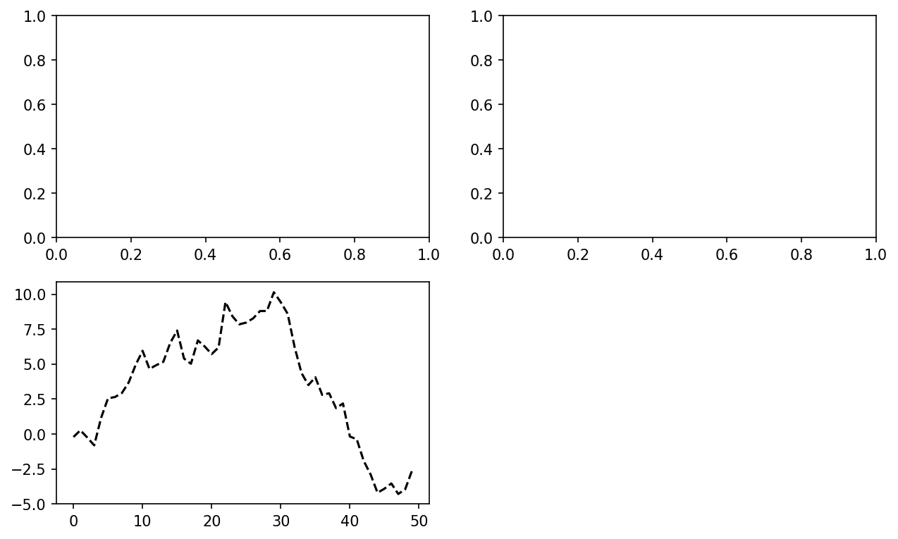
The 'k--' is a
style option instructing matplotlib to plot a black
dashed line. The objects returned by fig.add_subplot here are AxesSubplot
objects, on which you can directly plot on the other empty subplots by
calling each one’s instance method (see Figure 9-4):
In[21]:_=ax1.hist(np.random.randn(100),bins=20,color='k',alpha=0.3)In[22]:ax2.scatter(np.arange(30),np.arange(30)+3*np.random.randn(30))
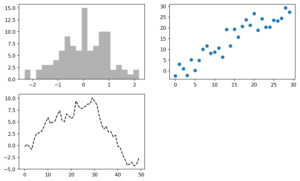
You can find a comprehensive catalog of plot types in the matplotlib documentation.
Creating a figure with a grid of subplots is a very common task,
so matplotlib includes a convenience method, plt.subplots, that creates a new figure and returns a NumPy array containing
the created subplot objects:
In[24]:fig,axes=plt.subplots(2,3)In[25]:axesOut[25]:array([[<matplotlib.axes._subplots.AxesSubplotobjectat0x7f435346c668>,<matplotlib.axes._subplots.AxesSubplotobjectat0x7f435338c780>,<matplotlib.axes._subplots.AxesSubplotobjectat0x7f43533c37f0>],[<matplotlib.axes._subplots.AxesSubplotobjectat0x7f435337d8d0>,<matplotlib.axes._subplots.AxesSubplotobjectat0x7f4353336908>,<matplotlib.axes._subplots.AxesSubplotobjectat0x7f43532ea400>]],dtype=object)
This is very useful, as the axes
array can be easily indexed like a two-dimensional array; for example,
axes[0, 1]. You can also indicate
that subplots should have the same x- or y-axis using sharex and sharey, respectively. This is especially
useful when you’re comparing data on the same scale; otherwise, matplotlib
autoscales plot limits independently. See Table 9-1 for more on this method.
| Argument | Description |
|---|---|
nrows | Number of rows of subplots |
ncols | Number of columns of subplots |
sharex | All subplots should use the same x-axis ticks (adjusting
the xlim will affect all
subplots) |
sharey | All subplots should use the same y-axis ticks (adjusting
the ylim will affect all
subplots) |
subplot_kw | Dict of keywords passed to add_subplot call used to create each
subplot |
**fig_kw | Additional keywords to subplots are used when creating the
figure, such as plt.subplots(2, 2, figsize=(8, 6)) |
By default matplotlib leaves a certain amount of padding around
the outside of the subplots and spacing between subplots. This spacing
is all specified relative to the height and width of the plot, so that
if you resize the plot either programmatically or manually using the
GUI window, the plot will dynamically adjust itself. You can change the spacing using the subplots_adjust method on Figure objects, also available as a
top-level function:
subplots_adjust(left=None, bottom=None, right=None, top=None,
wspace=None, hspace=None)wspace and hspace controls the percent of the figure
width and figure height, respectively, to use as spacing between
subplots. Here is a small example where I shrink the spacing all the
way to zero (see Figure 9-5):
fig,axes=plt.subplots(2,2,sharex=True,sharey=True)foriinrange(2):forjinrange(2):axes[i,j].hist(np.random.randn(500),bins=50,color='k',alpha=0.5)plt.subplots_adjust(wspace=0,hspace=0)
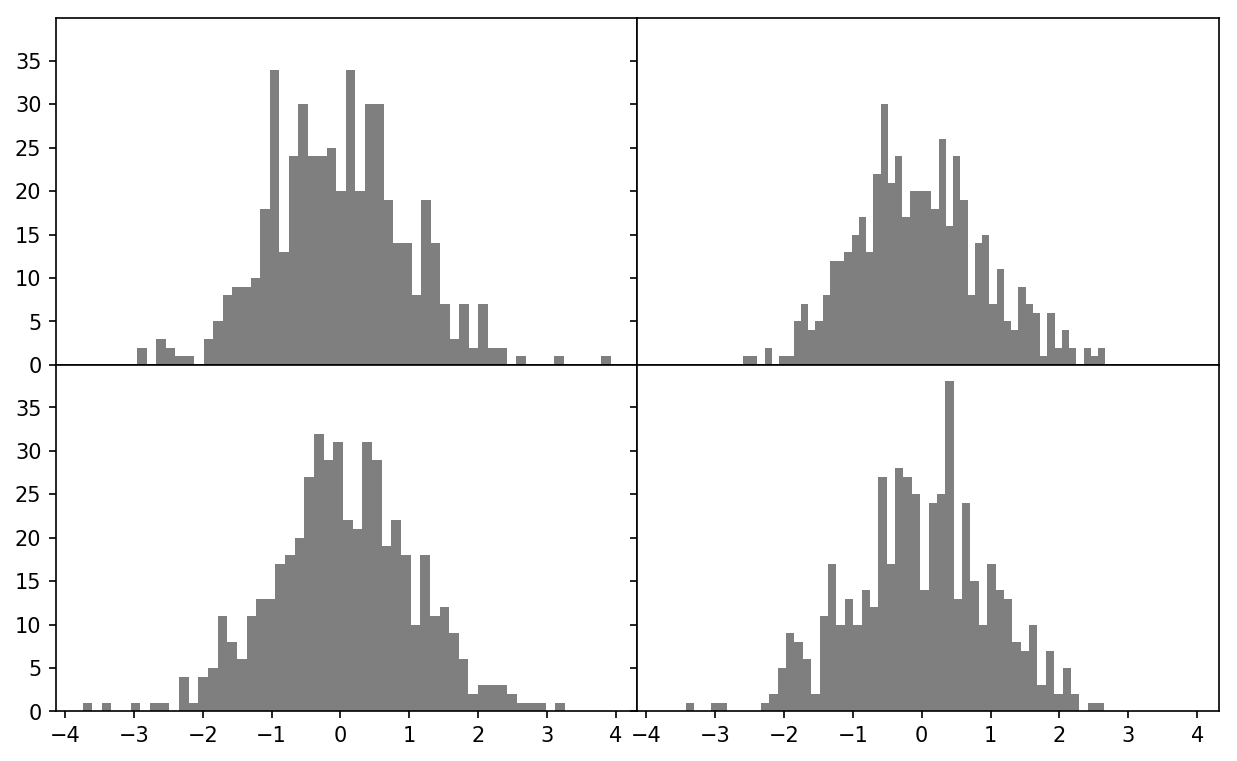
You may notice that the axis labels overlap. matplotlib doesn’t check whether the labels overlap, so in a case like this you would need to fix the labels yourself by specifying explicit tick locations and tick labels (we’ll look at how to do this in the following sections).
Matplotlib’s main plot function
accepts arrays of x and y coordinates and optionally a
string abbreviation indicating color and line style. For example, to
plot x versus y with green dashes, you would execute:
ax.plot(x,y,'g--')
This way of specifying both color and line style in a string is provided as a convenience; in practice if you were creating plots programmatically you might prefer not to have to munge strings together to create plots with the desired style. The same plot could also have been expressed more explicitly as:
ax.plot(x,y,linestyle='--',color='g')
There are a number of color abbreviations provided for commonly
used colors, but you can use any color on the spectrum by specifying its
hex code (e.g., '#CECECE'). You can
see the full set of line styles by looking at the docstring for plot (use plot? in IPython
or Jupyter).
Line plots can additionally have markers to highlight the actual data points. Since matplotlib creates a continuous line plot, interpolating between points, it can occasionally be unclear where the points lie. The marker can be part of the style string, which must have color followed by marker type and line style (see Figure 9-6):
In[30]:fromnumpy.randomimportrandnIn[31]:plt.plot(randn(30).cumsum(),'ko--')
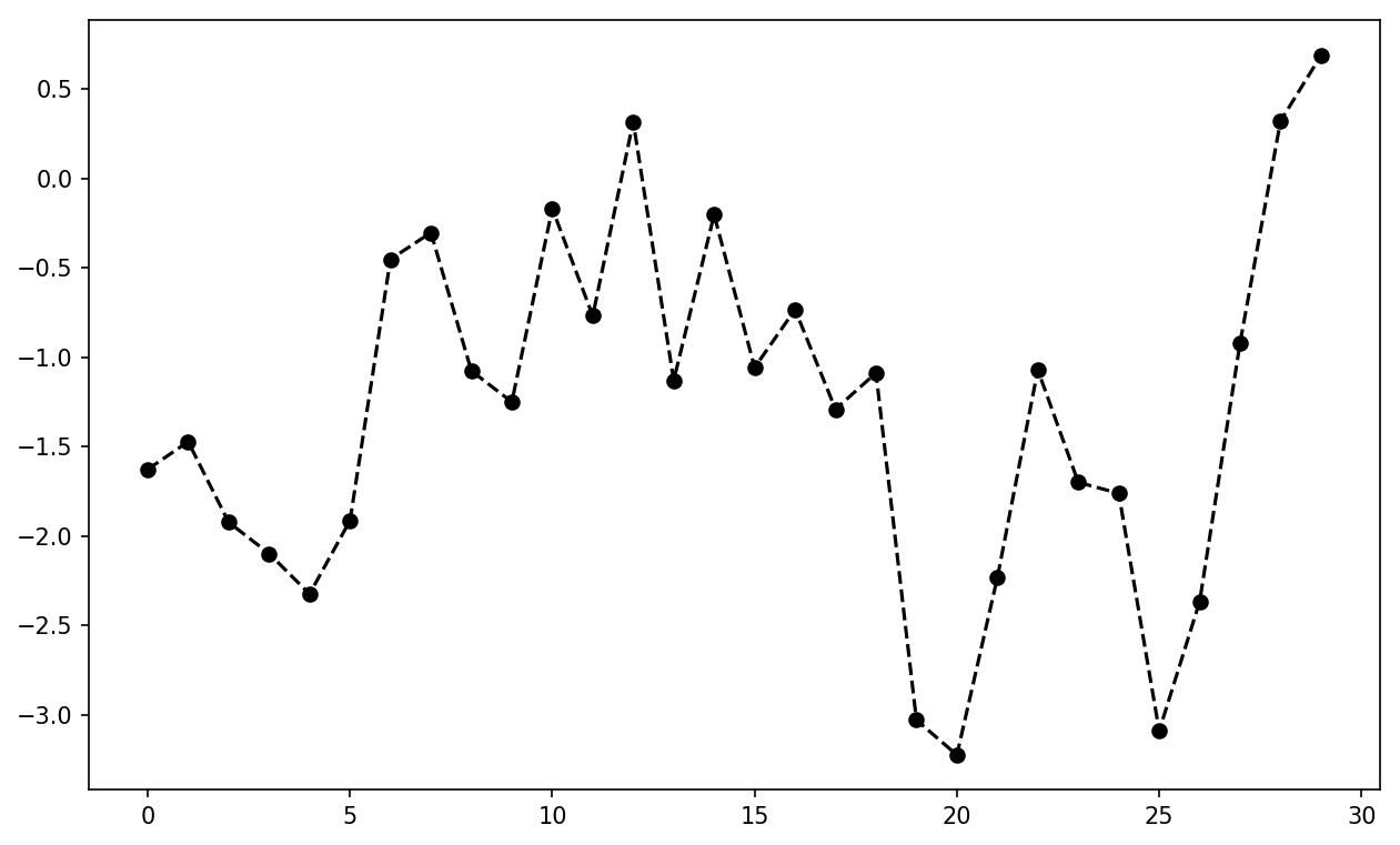
This could also have been written more explicitly as:
plot(randn(30).cumsum(),color='k',linestyle='dashed',marker='o')
For line plots, you will notice that subsequent points are
linearly interpolated by default. This can be altered with the drawstyle option (Figure 9-7):
In[33]:data=np.random.randn(30).cumsum()In[34]:plt.plot(data,'k--',label='Default')Out[34]:[<matplotlib.lines.Line2Dat0x7f43502adcf8>]In[35]:plt.plot(data,'k-',drawstyle='steps-post',label='steps-post')Out[35]:[<matplotlib.lines.Line2Dat0x7f43502b62e8>]In[36]:plt.legend(loc='best')
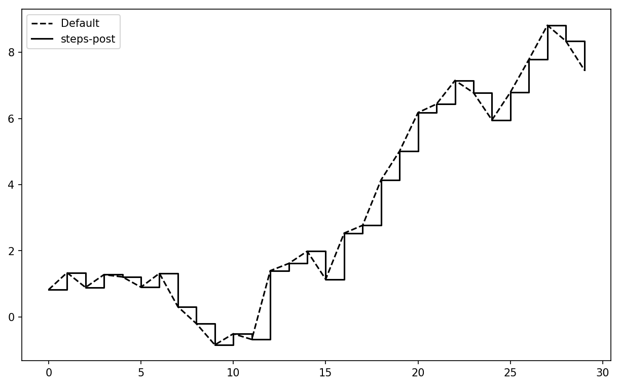
You may notice output like <matplotlib.lines.Line2D at
...> when you run this. matplotlib returns objects that
reference the plot subcomponent that was just added. A lot of the time
you can safely ignore this output. Here, since we passed the
label arguments to plot, we are
able to create a plot legend to identify each line using plt.legend.
You must call plt.legend (or
ax.legend, if you have a reference to the axes) to
create the legend, whether or not you passed the
label options when plotting the data.
For most kinds of plot decorations, there are two main ways to do things: using
the procedural pyplot
interface (i.e., matplotlib.pyplot) and the more
object-oriented native matplotlib API.
The pyplot interface, designed
for interactive use, consists of methods like xlim, xticks, and xticklabels. These control the plot range,
tick locations, and tick labels, respectively. They can be used in two
ways:
Called with no arguments returns the current parameter value
(e.g., plt.xlim() returns the
current x-axis plotting range)
Called with parameters sets the parameter value (e.g.,
plt.xlim([0, 10]), sets the x-axis range to 0 to 10)
All such methods act on the active or most recently created AxesSubplot.
Each of them corresponds to two methods on the subplot object itself; in the case of
xlim these are ax.get_xlim and ax.set_xlim. I prefer to use the subplot
instance methods myself in the interest of being explicit (and
especially when working with multiple subplots), but you can certainly
use whichever you find more convenient.
To illustrate customizing the axes, I’ll create a simple figure and plot of a random walk (see Figure 9-8):
In[37]:fig=plt.figure()In[38]:ax=fig.add_subplot(1,1,1)In[39]:ax.plot(np.random.randn(1000).cumsum())
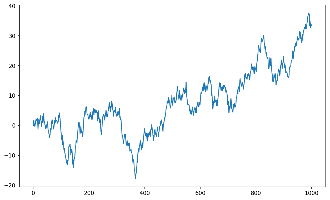
To change the x-axis ticks, it’s easiest to use set_xticks and
set_xticklabels. The former
instructs matplotlib where to place the ticks along the data range; by
default these locations will also be the labels. But we can set any
other values as the labels using set_xticklabels:
In[40]:ticks=ax.set_xticks([0,250,500,750,1000])In[41]:labels=ax.set_xticklabels(['one','two','three','four','five'],....:rotation=30,fontsize='small')
The rotation option sets the x tick labels at
a 30-degree rotation. Lastly, set_xlabel gives
a name to the x-axis and set_title the
subplot title (see Figure 9-9 for the resulting
figure):
In[42]:ax.set_title('My first matplotlib plot')Out[42]:Text(0.5,1,'My first matplotlib plot')In[43]:ax.set_xlabel('Stages')
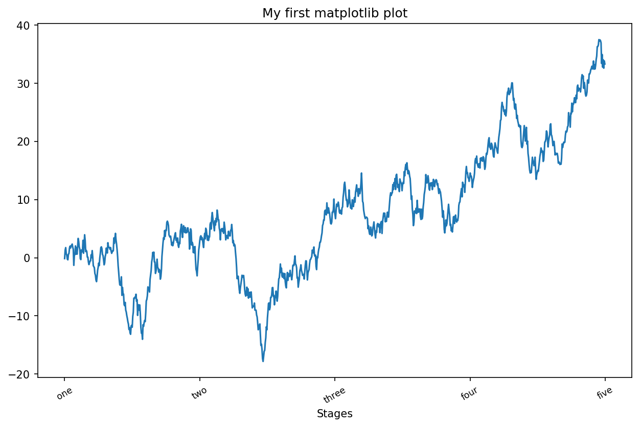
Modifying the y-axis consists of the same process, substituting
y for x in the above. The axes class has a set method that allows
batch setting of plot properties. From the prior example, we could
also have written:
props={'title':'My first matplotlib plot','xlabel':'Stages'}ax.set(**props)
Legends are another critical element for identifying plot
elements. There are a couple of ways to add one. The easiest is to
pass the label argument when adding
each piece of the plot:
In[44]:fromnumpy.randomimportrandnIn[45]:fig=plt.figure();ax=fig.add_subplot(1,1,1)In[46]:ax.plot(randn(1000).cumsum(),'k',label='one')Out[46]:[<matplotlib.lines.Line2Dat0x7f4350204da0>]In[47]:ax.plot(randn(1000).cumsum(),'k--',label='two')Out[47]:[<matplotlib.lines.Line2Dat0x7f435020e390>]In[48]:ax.plot(randn(1000).cumsum(),'k.',label='three')Out[48]:[<matplotlib.lines.Line2Dat0x7f435020e828>]
Once you’ve done this, you can either call ax.legend() or
plt.legend() to automatically
create a legend. The resulting plot is in Figure 9-10:
In[49]:ax.legend(loc='best')
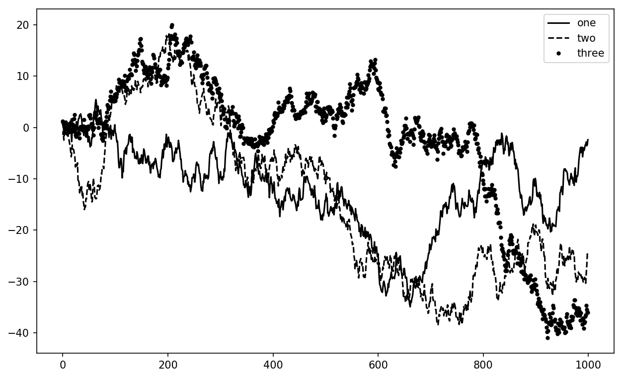
The legend method has several other choices
for the location loc argument. See the docstring
(with ax.legend?) for more information.
The loc tells matplotlib where to place the plot. If you aren’t picky,
'best' is a good option, as it will
choose a location that is most out of the way. To exclude one or more
elements from the legend, pass no label or label='_nolegend_'.
In addition to the standard plot types, you may wish to draw your own plot
annotations, which could consist of text, arrows, or other
shapes. You can add annotations and text using the text,
arrow, and annotate functions. text draws text at given coordinates (x, y) on the plot with optional custom
styling:
ax.text(x,y,'Hello world!',family='monospace',fontsize=10)
Annotations can draw both text and arrows arranged appropriately. As an example, let’s plot the closing S&P 500 index price since 2007 (obtained from Yahoo! Finance) and annotate it with some of the important dates from the 2008–2009 financial crisis. You can most easily reproduce this code example in a single cell in a Jupyter notebook. See Figure 9-11 for the result:
fromdatetimeimportdatetimefig=plt.figure()ax=fig.add_subplot(1,1,1)data=pd.read_csv('examples/spx.csv',index_col=0,parse_dates=True)spx=data['SPX']spx.plot(ax=ax,style='k-')crisis_data=[(datetime(2007,10,11),'Peak of bull market'),(datetime(2008,3,12),'Bear Stearns Fails'),(datetime(2008,9,15),'Lehman Bankruptcy')]fordate,labelincrisis_data:ax.annotate(label,xy=(date,spx.asof(date)+75),xytext=(date,spx.asof(date)+225),arrowprops=dict(facecolor='black',headwidth=4,width=2,headlength=4),horizontalalignment='left',verticalalignment='top')# Zoom in on 2007-2010ax.set_xlim(['1/1/2007','1/1/2011'])ax.set_ylim([600,1800])ax.set_title('Important dates in the 2008-2009 financial crisis')
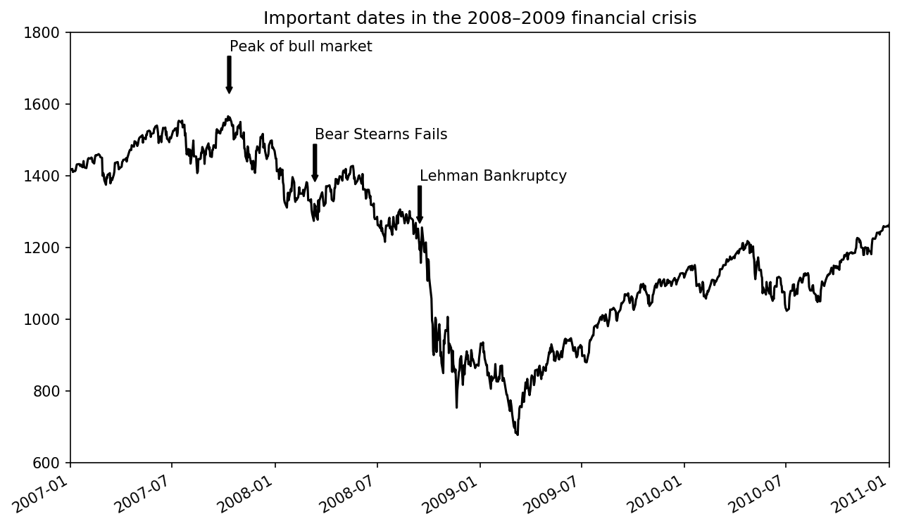
There are a couple of important points to highlight in this plot:
the ax.annotate method can draw labels at the
indicated x and y coordinates. We use the set_xlim and
set_ylim methods to manually set the start and end
boundaries for the plot rather than using matplotlib’s default. Lastly,
ax.set_title adds a main title to the plot.
See the online matplotlib gallery for many more annotation examples to learn from.
Drawing shapes requires some more care. matplotlib has objects
that represent many common shapes, referred to as patches. Some of these, like
Rectangle and Circle, are found in matplotlib.pyplot, but the full set is located
in matplotlib.patches.
To add a shape to a plot, you create the patch object shp and add it to a subplot by calling ax.add_patch(shp) (see Figure 9-12):
fig=plt.figure()ax=fig.add_subplot(1,1,1)rect=plt.Rectangle((0.2,0.75),0.4,0.15,color='k',alpha=0.3)circ=plt.Circle((0.7,0.2),0.15,color='b',alpha=0.3)pgon=plt.Polygon([[0.15,0.15],[0.35,0.4],[0.2,0.6]],color='g',alpha=0.5)ax.add_patch(rect)ax.add_patch(circ)ax.add_patch(pgon)
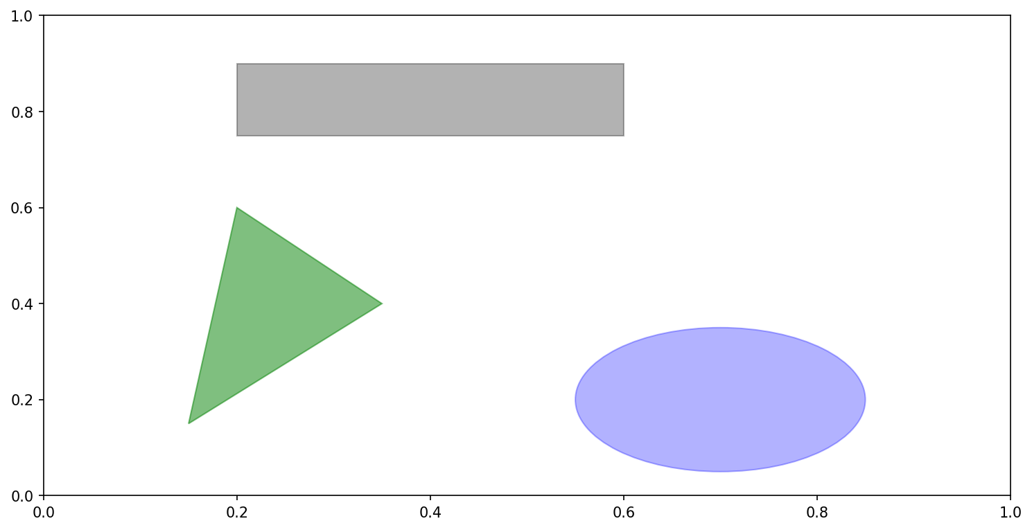
If you look at the implementation of many familiar plot types, you will see that they are assembled from patches.
You can save the active figure to file using plt.savefig. This method is equivalent to the
figure object’s savefig instance
method. For example, to save an SVG version of a figure,
you need only type:
plt.savefig('figpath.svg')
The file type is inferred from the file extension. So if you used
.pdf instead, you would get a PDF.
There are a couple of important options that I use frequently for
publishing graphics: dpi, which
controls the dots-per-inch resolution, and bbox_inches, which can trim the whitespace around the actual figure. To get the same plot
as a PNG with minimal whitespace around the plot and at 400 DPI, you
would do:
plt.savefig('figpath.png',dpi=400,bbox_inches='tight')
savefig doesn’t have to write
to disk; it can also write to any file-like object, such as a BytesIO:
fromioimportBytesIObuffer=BytesIO()plt.savefig(buffer)plot_data=buffer.getvalue()
See Table 9-2 for a list of some other
options for savefig.
| Argument | Description |
|---|---|
fname | String containing a filepath or a Python file-like
object. The figure format is inferred from the file extension
(e.g., .pdf for PDF or
.png for PNG) |
dpi | The figure resolution in dots per inch; defaults to 100 out of the box but can be configured |
facecolor, edgecolor | The color of the figure background outside of the
subplots; 'w' (white), by
default |
format | The explicit file format to use ('png', 'pdf', 'svg', 'ps', 'eps', ...) |
bbox_inches | The portion of the figure to save; if 'tight' is passed, will attempt to
trim the empty space around the figure |
matplotlib comes configured with color schemes and defaults that are geared
primarily toward preparing figures for publication. Fortunately, nearly
all of the default behavior can be customized via an extensive set of
global parameters governing figure size, subplot spacing, colors, font
sizes, grid styles, and so on. One way to modify the configuration
programmatically from Python is to use the rc method; for
example, to set the global default figure size to be 10 × 10, you could
enter:
plt.rc('figure',figsize=(10,10))
The first argument to rc is the
component you wish to customize, such as 'figure', 'axes', 'xtick', 'ytick', 'grid', 'legend', or many
others. After that can follow a sequence of keyword arguments indicating
the new parameters. An easy way to write down the options in your
program is as a dict:
font_options={'family':'monospace','weight':'bold','size':'small'}plt.rc('font',**font_options)
For more extensive customization and to see a list of all the options, matplotlib comes with a configuration file matplotlibrc in the matplotlib/mpl-data directory. If you customize this file and place it in your home directory titled .matplotlibrc, it will be loaded each time you use matplotlib.
As we’ll see in the next section, the seaborn package has several built-in plot themes or styles that use matplotlib’s configuration system internally.
matplotlib can be a fairly low-level tool. You assemble a plot from its base components: the data display (i.e., the type of plot: line, bar, box, scatter, contour, etc.), legend, title, tick labels, and other annotations.
In pandas we may have multiple columns of data, along with row and
column labels. pandas itself has built-in methods that simplify creating
visualizations from DataFrame and Series objects. Another library is
seaborn, a
statistical graphics library created by Michael Waskom. Seaborn simplifies creating many common
visualization types.
Importing seaborn modifies the default matplotlib color schemes and plot styles to improve readability and aesthetics. Even if you do not use the seaborn API, you may prefer to import seaborn as a simple way to improve the visual aesthetics of general matplotlib plots.
Series and DataFrame each have a plot attribute for making some basic plot
types. By default, plot() makes line plots (see Figure 9-13):
In[60]:s=pd.Series(np.random.randn(10).cumsum(),index=np.arange(0,100,10))In[61]:s.plot()
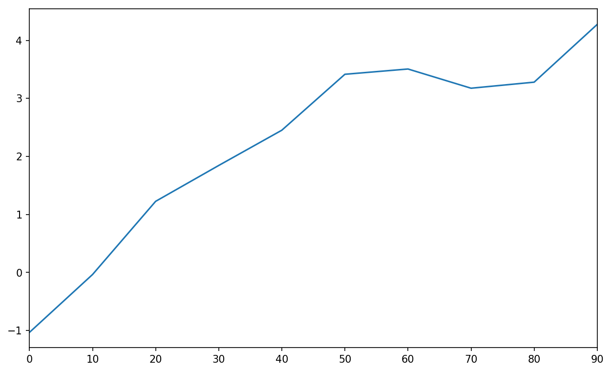
The Series object’s index is passed to matplotlib for plotting on
the x-axis, though you can disable this by passing use_index=False. The x-axis ticks and limits
can be adjusted with the xticks and
xlim options, and y-axis respectively
with yticks and ylim. See Table 9-3
for a full listing of plot options.
I’ll comment on a few more of them throughout this section and leave the
rest to you to explore.
Most of pandas’s plotting methods accept an optional ax parameter, which can be a matplotlib
subplot object. This gives you more flexible placement of subplots in a
grid layout.
DataFrame’s plot method plots
each of its columns as a different line on the same subplot, creating a
legend automatically (see Figure 9-14):
In[62]:df=pd.DataFrame(np.random.randn(10,4).cumsum(0),....:columns=['A','B','C','D'],....:index=np.arange(0,100,10))In[63]:df.plot()
The plot attribute contains a “family” of
methods for different plot types. For example,
df.plot() is equivalent to
df.plot.line(). We’ll explore some of these methods
next.
Additional keyword arguments to plot are passed through to the respective
matplotlib plotting function, so you can further customize these plots
by learning more about the matplotlib API.
DataFrame has a number of options allowing some flexibility with how the columns are handled; for example, whether to plot them all on the same subplot or to create separate subplots. See Table 9-4 for more on these.
For time series plotting, see Chapter 11.
The plot.bar() and
plot.barh() make vertical and horizontal bar plots, respectively. In this
case, the Series or DataFrame index will be used as the x (bar) or y (barh) ticks (see Figure 9-15):
In[64]:fig,axes=plt.subplots(2,1)In[65]:data=pd.Series(np.random.rand(16),index=list('abcdefghijklmnop'))In[66]:data.plot.bar(ax=axes[0],color='k',alpha=0.7)Out[66]:<matplotlib.axes._subplots.AxesSubplotat0x7f43500afc18>In[67]:data.plot.barh(ax=axes[1],color='k',alpha=0.7)
The options color='k' and
alpha=0.7 set the color of the plots to black and use
partial transparency on the filling.
With a DataFrame, bar plots group the values in each row together in a group in bars, side by side, for each value. See Figure 9-16:
In[69]:df=pd.DataFrame(np.random.rand(6,4),....:index=['one','two','three','four','five','six'],....:columns=pd.Index(['A','B','C','D'],name='Genus'))In[70]:dfOut[70]:GenusABCDone0.3706700.6027920.2291590.486744two0.4200820.5716530.0490240.880592three0.8145680.2771600.8803160.431326four0.3740200.8994200.4603040.100843five0.4332700.1251070.4946750.961825six0.6016480.4785760.2056900.560547In[71]:df.plot.bar()
Note that the name “Genus” on the DataFrame’s columns is used to title the legend.
We create stacked bar plots from a DataFrame by passing stacked=True, resulting in the value in each
row being stacked together (see Figure 9-17):
In[73]:df.plot.barh(stacked=True,alpha=0.5)
A useful recipe for bar plots is to visualize a Series’s value
frequency using value_counts:
s.value_counts().plot.bar().
Returning to the tipping dataset used earlier in the book, suppose
we wanted to make a stacked bar plot showing the percentage of data
points for each party size on each day. I load the data using read_csv and make
a cross-tabulation by day and party size:
In[75]:tips=pd.read_csv('examples/tips.csv')In[76]:party_counts=pd.crosstab(tips['day'],tips['size'])In[77]:party_countsOut[77]:size123456dayFri1161100Sat253181310Sun039151831Thur1484513# Not many 1- and 6-person partiesIn[78]:party_counts=party_counts.loc[:,2:5]
Then, normalize so that each row sums to 1 and make the plot (see Figure 9-18):
# Normalize to sum to 1In[79]:party_pcts=party_counts.div(party_counts.sum(1),axis=0)In[80]:party_pctsOut[80]:size2345dayFri0.8888890.0555560.0555560.000000Sat0.6235290.2117650.1529410.011765Sun0.5200000.2000000.2400000.040000Thur0.8275860.0689660.0862070.017241In[81]:party_pcts.plot.bar()
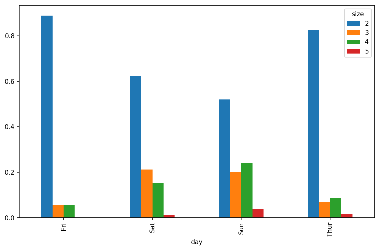
So you can see that party sizes appear to increase on the weekend in this dataset.
With data that requires aggregation or summarization before making
a plot, using the seaborn package can make things
much simpler. Let’s look now at the tipping percentage by day with
seaborn (see Figure 9-19 for the resulting
plot):
In[83]:importseabornassnsIn[84]:tips['tip_pct']=tips['tip']/(tips['total_bill']-tips['tip'])In[85]:tips.head()Out[85]:total_billtipsmokerdaytimesizetip_pct016.991.01NoSunDinner20.063204110.341.66NoSunDinner30.191244221.013.50NoSunDinner30.199886323.683.31NoSunDinner20.162494424.593.61NoSunDinner40.172069In[86]:sns.barplot(x='tip_pct',y='day',data=tips,orient='h')
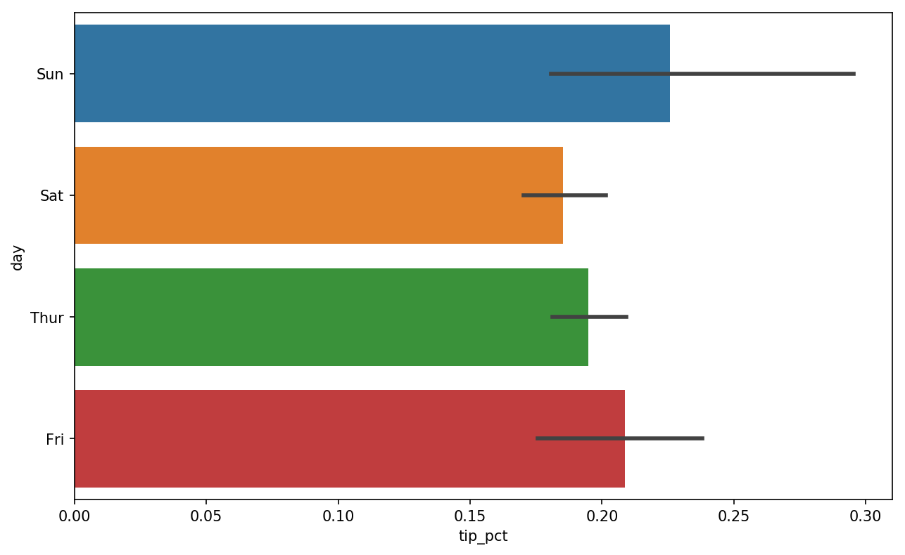
Plotting functions in seaborn take a data
argument, which can be a pandas DataFrame. The other arguments refer to
column names. Because there are multiple observations for each value in
the day, the bars are the average value of
tip_pct. The black lines drawn on the bars represent
the 95% confidence interval (this can be configured through optional
arguments).
seaborn.barplot has a hue option that enables us to
split by an additional categorical value (Figure 9-20):
In[88]:sns.barplot(x='tip_pct',y='day',hue='time',data=tips,orient='h')
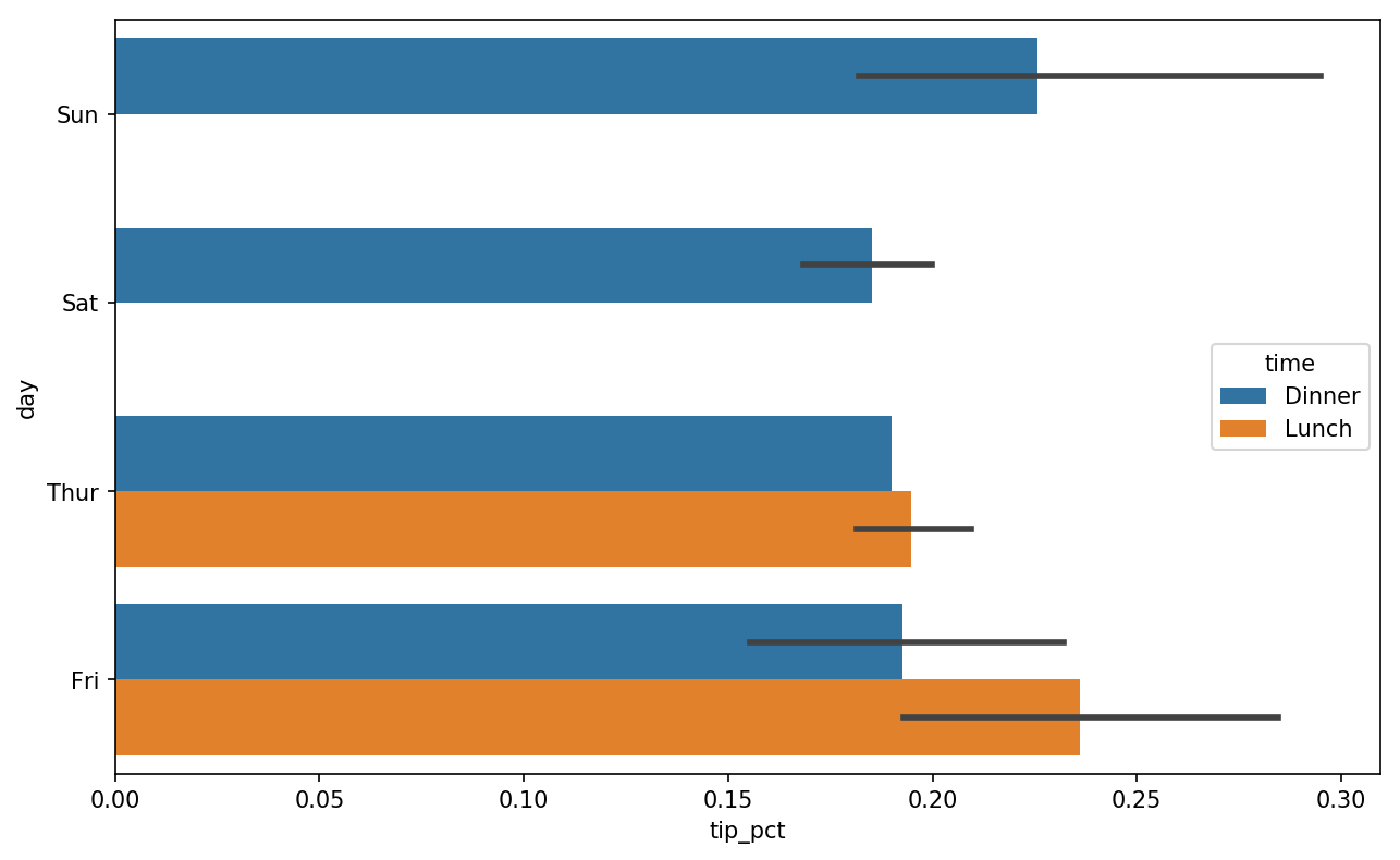
Notice that seaborn has automatically changed the aesthetics of
plots: the default color palette, plot background, and grid line colors.
You can switch between different plot appearances using seaborn.set:
In[90]:sns.set(style="whitegrid")
A histogram is a kind of bar plot that gives a discretized display of value
frequency. The data points are split into discrete, evenly spaced bins,
and the number of data points in each bin is plotted. Using the tipping
data from before, we can make a histogram of tip percentages of the
total bill using the plot.hist method
on the Series (see Figure 9-21):
In[92]:tips['tip_pct'].plot.hist(bins=50)
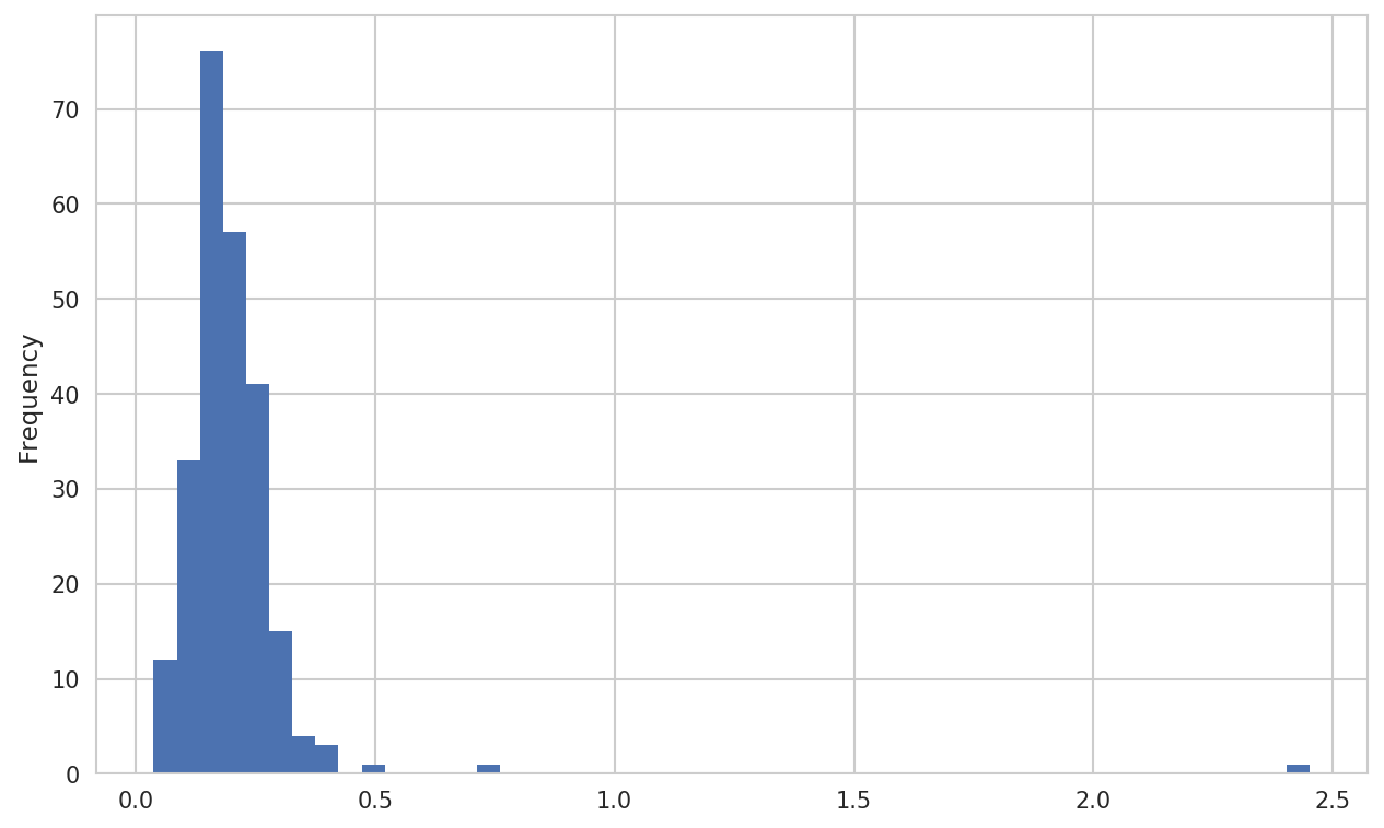
A related plot type is a density plot, which
is formed by computing an estimate of a continuous probability
distribution that might have generated the observed data. The usual
procedure is to approximate this distribution as a mixture of “kernels”—that is, simpler distributions like the normal distribution. Thus,
density plots are also known as kernel density estimate (KDE) plots. Using plot.kde makes a density plot using the
conventional mixture-of-normals estimate (see Figure 9-22):
In[94]:tips['tip_pct'].plot.density()
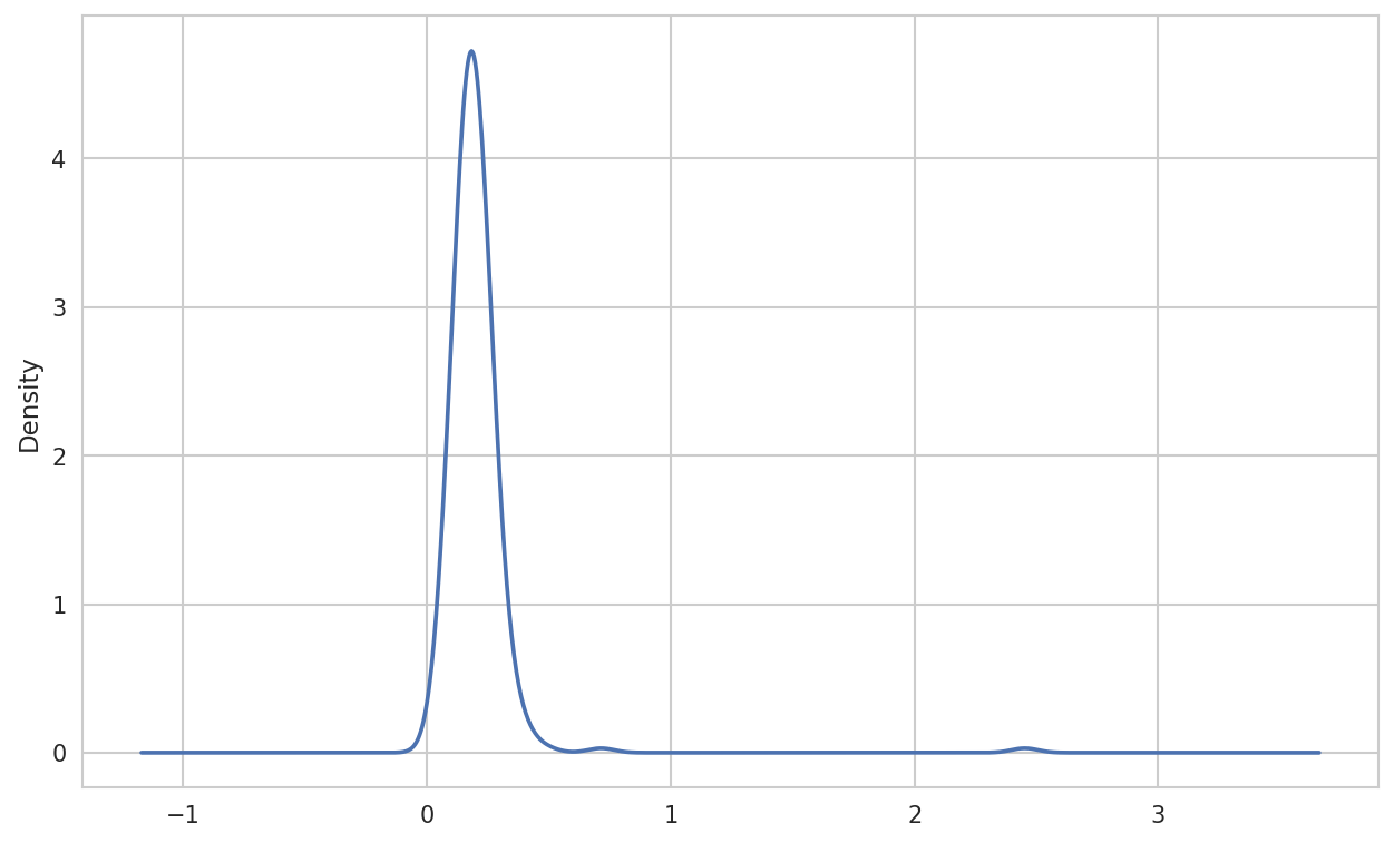
Seaborn makes histograms and density plots even easier through its distplot method, which can
plot both a histogram and a continuous density estimate simultaneously.
As an example, consider a bimodal distribution consisting of draws from
two different standard normal distributions (see Figure 9-23):
In[96]:comp1=np.random.normal(0,1,size=200)In[97]:comp2=np.random.normal(10,2,size=200)In[98]:values=pd.Series(np.concatenate([comp1,comp2]))In[99]:sns.distplot(values,bins=100,color='k')
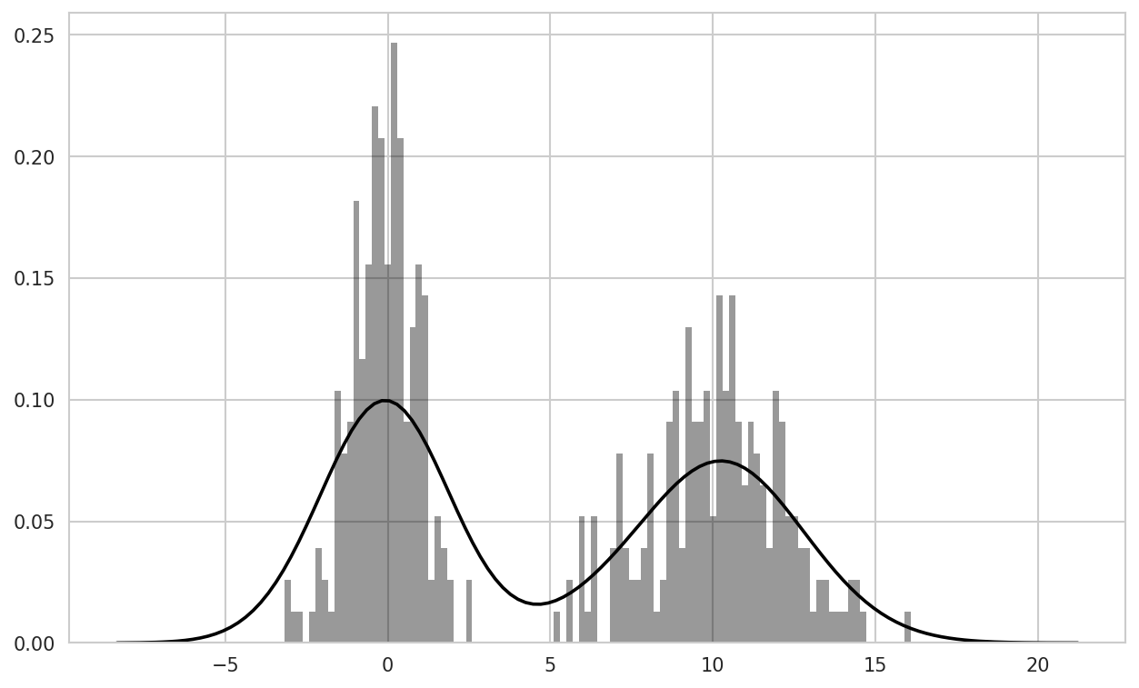
Point plots or scatter plots can be a useful way of examining the
relationship between two one-dimensional data series. For example, here
we load the macrodata dataset from
the statsmodels project, select a few variables, then compute log
differences:
In[100]:macro=pd.read_csv('examples/macrodata.csv')In[101]:data=macro[['cpi','m1','tbilrate','unemp']]In[102]:trans_data=np.log(data).diff().dropna()In[103]:trans_data[-5:]Out[103]:cpim1tbilrateunemp198-0.0079040.045361-0.3968810.105361199-0.0219790.066753-2.2772670.1397622000.0023400.0102860.6061360.1603432010.0084190.037461-0.2006710.1273392020.0088940.012202-0.4054650.042560
We can then use seaborn’s regplot method, which makes a
scatter plot and fits a linear regression line (see Figure 9-24):
In[105]:sns.regplot('m1','unemp',data=trans_data)Out[105]:<matplotlib.axes._subplots.AxesSubplotat0x7f4341097cf8>In[106]:plt.title('Changes in log%sversus log%s'%('m1','unemp'))

In exploratory data analysis it’s helpful to be able to look at
all the scatter plots among a group of variables; this is known
as a pairs plot or scatter
plot matrix. Making such a plot from scratch is a bit of
work, so seaborn has a convenient pairplot function, which
supports placing histograms or density estimates of each variable along
the diagonal (see Figure 9-25 for the resulting
plot):
In[107]:sns.pairplot(trans_data,diag_kind='kde',plot_kws={'alpha':0.2})
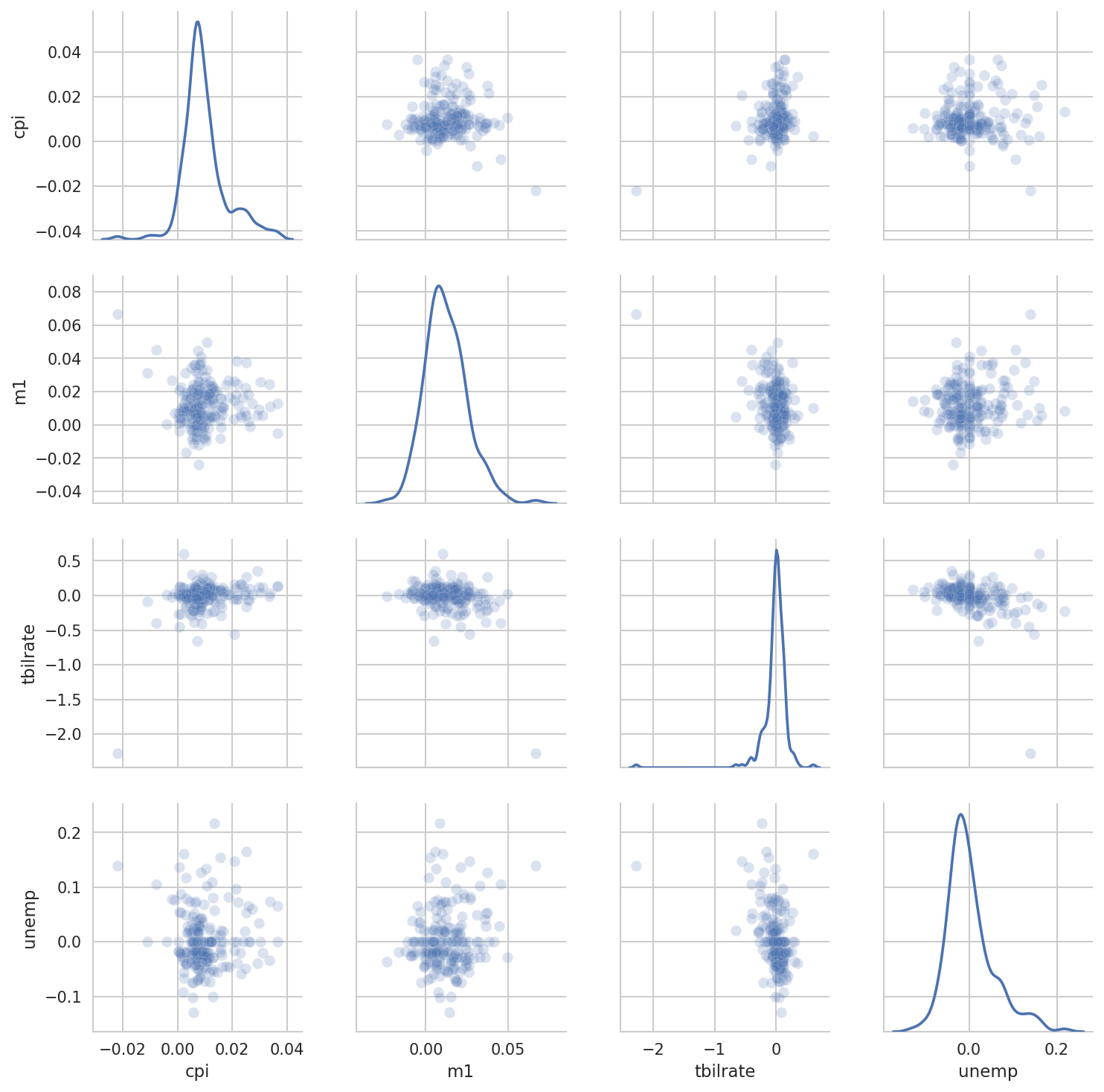
You may notice the plot_kws argument. This
enables us to pass down configuration options to the individual plotting
calls on the off-diagonal elements. Check out the
seaborn.pairplot docstring for more granular
configuration options.
What about datasets where we have additional grouping dimensions? One way to
visualize data with many categorical variables is to use a
facet grid. Seaborn has a useful built-in function
factorplot that simplifies making many kinds of faceted plots (see Figure 9-26 for the resulting plot):
In[108]:sns.factorplot(x='day',y='tip_pct',hue='time',col='smoker',.....:kind='bar',data=tips[tips.tip_pct<1])
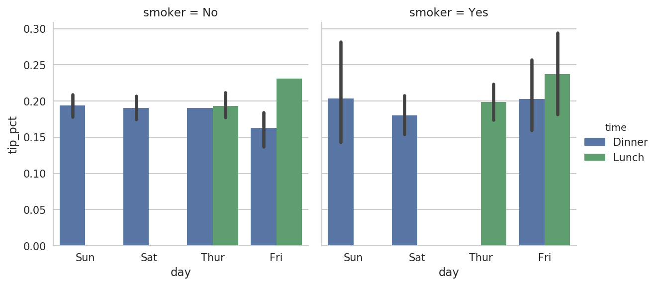
Instead of grouping by 'time' by different bar
colors within a facet, we can also expand the facet grid by adding one
row per time value (Figure 9-27):
In[109]:sns.factorplot(x='day',y='tip_pct',row='time',.....:col='smoker',.....:kind='bar',data=tips[tips.tip_pct<1])
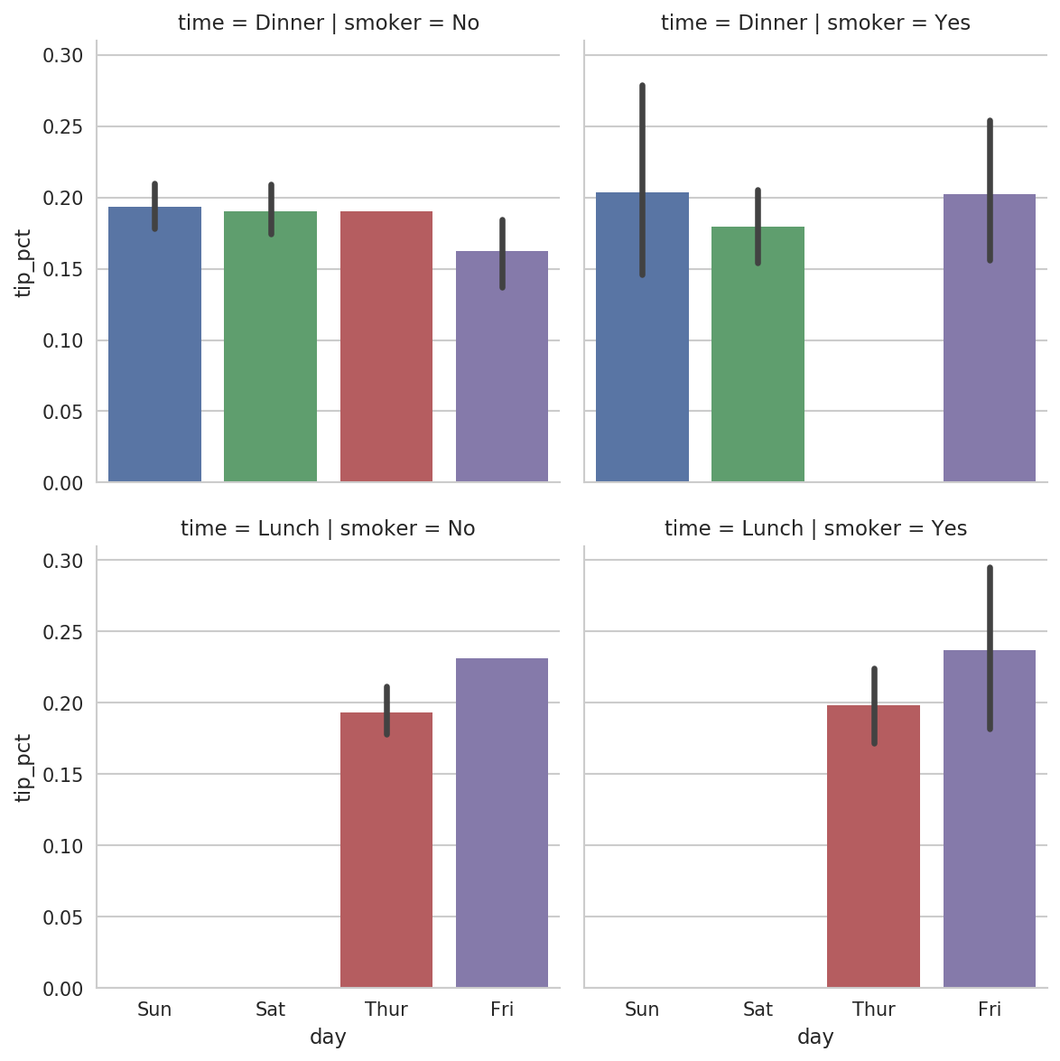
factorplot supports other plot types that may
be useful depending on what you are trying to display. For example, box
plots (which show the median, quartiles, and outliers) can be an
effective visualization type (Figure 9-28):
In[110]:sns.factorplot(x='tip_pct',y='day',kind='box',.....:data=tips[tips.tip_pct<0.5])
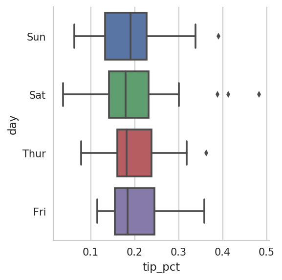
You can create your own facet grid plots using the more general seaborn.FacetGrid class. See
the seaborn
documentation for more.
As is common with open source, there are a plethora of options for creating graphics in Python (too many to list). Since 2010, much development effort has been focused on creating interactive graphics for publication on the web. With tools like Bokeh and Plotly, it’s now possible to specify dynamic, interactive graphics in Python that are destined for a web browser.
For creating static graphics for print or web, I recommend defaulting to matplotlib and add-on libraries like pandas and seaborn for your needs. For other data visualization requirements, it may be useful to learn one of the other available tools out there. I encourage you to explore the ecosystem as it continues to involve and innovate into the future.
The goal of this chapter was to get your feet wet with some basic data visualization using pandas, matplotlib, and seaborn. If visually communicating the results of data analysis is important in your work, I encourage you to seek out resources to learn more about effective data visualization. It is an active field of research and you can practice with many excellent learning resources available online and in print form.
In the next chapter, we turn our attention to data aggregation and group operations with pandas.
Categorizing a dataset and applying a function to each group, whether an
aggregation or transformation, is often a critical component of a data
analysis workflow. After loading, merging, and preparing a dataset, you may
need to compute group statistics or possibly pivot tables for reporting or
visualization purposes. pandas provides a flexible groupby interface, enabling you to slice, dice,
and summarize datasets in a natural way.
One reason for the popularity of relational databases and SQL (which stands for “structured query language”) is the ease with which data can be joined, filtered, transformed, and aggregated. However, query languages like SQL are somewhat constrained in the kinds of group operations that can be performed. As you will see, with the expressiveness of Python and pandas, we can perform quite complex group operations by utilizing any function that accepts a pandas object or NumPy array. In this chapter, you will learn how to:
Split a pandas object into pieces using one or more keys (in the form of functions, arrays, or DataFrame column names)
Calculate group summary statistics, like count, mean, or standard deviation, or a user-defined function
Apply within-group transformations or other manipulations, like normalization, linear regression, rank, or subset selection
Compute pivot tables and cross-tabulations
Perform quantile analysis and other statistical group analyses
Aggregation of time series data, a special use case of groupby, is referred to as
resampling in this book and will receive separate
treatment in Chapter 11.
Hadley Wickham, an author of many popular packages for the R programming
language, coined the term split-apply-combine for
describing group operations. In the first stage of the
process, data contained in a pandas object, whether a Series, DataFrame,
or otherwise, is split into groups based on one or
more keys that you provide. The splitting is
performed on a particular axis of an object. For example, a DataFrame can
be grouped on its rows (axis=0) or its
columns (axis=1). Once this is done, a
function is applied to each group, producing a new
value. Finally, the results of all those function applications are
combined into a result object. The form of the
resulting object will usually depend on what’s being done to the data. See
Figure 10-1 for a mockup of a simple group
aggregation.
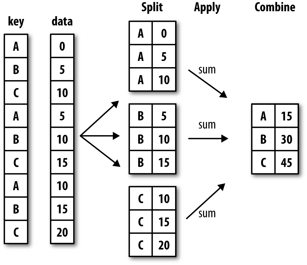
Each grouping key can take many forms, and the keys do not have to be all of the same type:
A list or array of values that is the same length as the axis being grouped
A value indicating a column name in a DataFrame
A dict or Series giving a correspondence between the values on the axis being grouped and the group names
A function to be invoked on the axis index or the individual labels in the index
Note that the latter three methods are shortcuts for producing an array of values to be used to split up the object. Don’t worry if this all seems abstract. Throughout this chapter, I will give many examples of all these methods. To get started, here is a small tabular dataset as a DataFrame:
In[10]:df=pd.DataFrame({'key1':['a','a','b','b','a'],....:'key2':['one','two','one','two','one'],....:'data1':np.random.randn(5),....:'data2':np.random.randn(5)})In[11]:dfOut[11]:data1data2key1key20-0.2047081.393406aone10.4789430.092908atwo2-0.5194390.281746bone3-0.5557300.769023btwo41.9657811.246435aone
Suppose you wanted to compute the mean of the data1 column using the labels from key1. There are a number of ways to do this. One
is to access data1 and call groupby with the column (a Series) at key1:
In[12]:grouped=df['data1'].groupby(df['key1'])In[13]:groupedOut[13]:<pandas.core.groupby.SeriesGroupByobjectat0x7f85008d0400>
This grouped variable is now a
GroupBy object. It has not actually computed anything
yet except for some intermediate data about the group key df['key1']. The idea is that this object has all
of the information needed to then apply some operation to each of the
groups. For example, to compute group means we can call the GroupBy’s mean
method:
In[14]:grouped.mean()Out[14]:key1a0.746672b-0.537585Name:data1,dtype:float64
Later, I’ll explain more about what happens when you call .mean(). The important thing here is that the
data (a Series) has been aggregated according to the group key, producing
a new Series that is now indexed by the unique values in the key1 column. The result index has the name
'key1' because the DataFrame column
df['key1'] did.
If instead we had passed multiple arrays as a list, we’d get something different:
In[15]:means=df['data1'].groupby([df['key1'],df['key2']]).mean()In[16]:meansOut[16]:key1key2aone0.880536two0.478943bone-0.519439two-0.555730Name:data1,dtype:float64
Here we grouped the data using two keys, and the resulting Series now has a hierarchical index consisting of the unique pairs of keys observed:
In[17]:means.unstack()Out[17]:key2onetwokey1a0.8805360.478943b-0.519439-0.555730
In this example, the group keys are all Series, though they could be any arrays of the right length:
In[18]:states=np.array(['Ohio','California','California','Ohio','Ohio'])In[19]:years=np.array([2005,2005,2006,2005,2006])In[20]:df['data1'].groupby([states,years]).mean()Out[20]:California20050.4789432006-0.519439Ohio2005-0.38021920061.965781Name:data1,dtype:float64
Frequently the grouping information is found in the same DataFrame as the data you want to work on. In that case, you can pass column names (whether those are strings, numbers, or other Python objects) as the group keys:
In[21]:df.groupby('key1').mean()Out[21]:data1data2key1a0.7466720.910916b-0.5375850.525384In[22]:df.groupby(['key1','key2']).mean()Out[22]:data1data2key1key2aone0.8805361.319920two0.4789430.092908bone-0.5194390.281746two-0.5557300.769023
You may have noticed in the first case df.groupby('key1').mean() that there is no
key2 column in the result. Because
df['key2'] is not numeric data, it is
said to be a nuisance column, which is therefore
excluded from the result. By default, all of the numeric columns are aggregated, though it is
possible to filter down to a subset, as you’ll see soon.
Regardless of the objective in using groupby, a generally useful GroupBy method is size,
which returns a Series containing group sizes:
In[23]:df.groupby(['key1','key2']).size()Out[23]:key1key2aone2two1bone1two1dtype:int64
Take note that any missing values in a group key will be excluded from the result.
The GroupBy object supports iteration, generating a sequence of 2-tuples containing the group name along with the chunk of data. Consider the following:
In[24]:forname,groupindf.groupby('key1'):....:(name)....:(group)....:adata1data2key1key20-0.2047081.393406aone10.4789430.092908atwo41.9657811.246435aonebdata1data2key1key22-0.5194390.281746bone3-0.5557300.769023btwo
In the case of multiple keys, the first element in the tuple will be a tuple of key values:
In[25]:for(k1,k2),groupindf.groupby(['key1','key2']):....:((k1,k2))....:(group)....:('a','one')data1data2key1key20-0.2047081.393406aone41.9657811.246435aone('a','two')data1data2key1key210.4789430.092908atwo('b','one')data1data2key1key22-0.5194390.281746bone('b','two')data1data2key1key23-0.555730.769023btwo
Of course, you can choose to do whatever you want with the pieces of data. A recipe you may find useful is computing a dict of the data pieces as a one-liner:
In[26]:pieces=dict(list(df.groupby('key1')))In[27]:pieces['b']Out[27]:data1data2key1key22-0.5194390.281746bone3-0.5557300.769023btwo
By default groupby groups on
axis=0, but you can group on any of
the other axes. For example, we could group the columns of our example
df here by dtype like so:
In[28]:df.dtypesOut[28]:data1float64data2float64key1objectkey2objectdtype:objectIn[29]:grouped=df.groupby(df.dtypes,axis=1)
We can print out the groups like so:
In[30]:fordtype,groupingrouped:....:(dtype)....:(group)....:float64data1data20-0.2047081.39340610.4789430.0929082-0.5194390.2817463-0.5557300.76902341.9657811.246435objectkey1key20aone1atwo2bone3btwo4aone
Indexing a GroupBy object created from a DataFrame with a column name or array of column names has the effect of column subsetting for aggregation. This means that:
df.groupby('key1')['data1']df.groupby('key1')[['data2']]
are syntactic sugar for:
df['data1'].groupby(df['key1'])df[['data2']].groupby(df['key1'])
Especially for large datasets, it may be desirable to aggregate
only a few columns. For example, in the preceding dataset, to compute
means for just the data2 column and
get the result as a DataFrame, we could write:
In[31]:df.groupby(['key1','key2'])[['data2']].mean()Out[31]:data2key1key2aone1.319920two0.092908bone0.281746two0.769023
The object returned by this indexing operation is a grouped DataFrame if a list or array is passed or a grouped Series if only a single column name is passed as a scalar:
In[32]:s_grouped=df.groupby(['key1','key2'])['data2']In[33]:s_groupedOut[33]:<pandas.core.groupby.SeriesGroupByobjectat0x7f85008983c8>In[34]:s_grouped.mean()Out[34]:key1key2aone1.319920two0.092908bone0.281746two0.769023Name:data2,dtype:float64
Grouping information may exist in a form other than an array. Let’s consider another example DataFrame:
In[35]:people=pd.DataFrame(np.random.randn(5,5),....:columns=['a','b','c','d','e'],....:index=['Joe','Steve','Wes','Jim','Travis'])In[36]:people.iloc[2:3,[1,2]]=np.nan# Add a few NA valuesIn[37]:peopleOut[37]:abcdeJoe1.007189-1.2962210.2749920.2289131.352917Steve0.886429-2.001637-0.3718431.669025-0.438570Wes-0.539741NaNNaN-1.021228-0.577087Jim0.1241210.3026140.5237720.0009401.343810Travis-0.713544-0.831154-2.370232-1.860761-0.860757
Now, suppose I have a group correspondence for the columns and want to sum together the columns by group:
In[38]:mapping={'a':'red','b':'red','c':'blue',....:'d':'blue','e':'red','f':'orange'}
Now, you could construct an array from this dict to pass to
groupby, but instead we can just pass
the dict (I included the key 'f' to highlight that
unused grouping keys are OK):
In[39]:by_column=people.groupby(mapping,axis=1)In[40]:by_column.sum()Out[40]:blueredJoe0.5039051.063885Steve1.297183-1.553778Wes-1.021228-1.116829Jim0.5247121.770545Travis-4.230992-2.405455
The same functionality holds for Series, which can be viewed as a fixed-size mapping:
In[41]:map_series=pd.Series(mapping)In[42]:map_seriesOut[42]:aredbredcbluedblueeredforangedtype:objectIn[43]:people.groupby(map_series,axis=1).count()Out[43]:blueredJoe23Steve23Wes12Jim23Travis23
Using Python functions is a more generic way of defining a group
mapping compared with a dict or Series. Any function passed as a group
key will be called once per index value, with the return values being
used as the group names. More concretely, consider the example DataFrame
from the previous section, which has people’s first names as index
values. Suppose you wanted to group by the length of the names; while
you could compute an array of string lengths, it’s simpler to just pass
the len
function:
In[44]:people.groupby(len).sum()Out[44]:abcde30.591569-0.9936080.798764-0.7913742.11963950.886429-2.001637-0.3718431.669025-0.4385706-0.713544-0.831154-2.370232-1.860761-0.860757
Mixing functions with arrays, dicts, or Series is not a problem as everything gets converted to arrays internally:
In[45]:key_list=['one','one','one','two','two']In[46]:people.groupby([len,key_list]).min()Out[46]:abcde3one-0.539741-1.2962210.274992-1.021228-0.577087two0.1241210.3026140.5237720.0009401.3438105one0.886429-2.001637-0.3718431.669025-0.4385706two-0.713544-0.831154-2.370232-1.860761-0.860757
A final convenience for hierarchically indexed datasets is the ability to aggregate using one of the levels of an axis index. Let’s look at an example:
In[47]:columns=pd.MultiIndex.from_arrays([['US','US','US','JP','JP'],....:[1,3,5,1,3]],....:names=['cty','tenor'])In[48]:hier_df=pd.DataFrame(np.random.randn(4,5),columns=columns)In[49]:hier_dfOut[49]:ctyUSJPtenor1351300.560145-1.2659340.119827-1.0635120.3328831-2.359419-0.199543-1.541996-0.970736-1.30703020.2863500.377984-0.7538870.3312861.34974230.0698770.246674-0.0118621.0048121.327195
To group by level, pass the level number or name using the level
keyword:
In[50]:hier_df.groupby(level='cty',axis=1).count()Out[50]:ctyJPUS023123223323
Aggregations refer to any data transformation that produces scalar values from arrays.
The preceding examples have used several of them, including mean, count, min, and sum. You may wonder what is going on when you
invoke mean() on a GroupBy object. Many
common aggregations, such as those found in Table 10-1, have optimized implementations. However, you are not limited to
only this set of methods.
You can use aggregations of your own devising and additionally call
any method that is also defined on the grouped object. For example, you
might recall that quantile computes
sample quantiles of a Series or a DataFrame’s columns.
While quantile is not explicitly
implemented for GroupBy, it is a Series method and thus available for use.
Internally, GroupBy efficiently slices up the Series, calls piece.quantile(0.9) for each piece, and then
assembles those results together into the result object:
In[51]:dfOut[51]:data1data2key1key20-0.2047081.393406aone10.4789430.092908atwo2-0.5194390.281746bone3-0.5557300.769023btwo41.9657811.246435aoneIn[52]:grouped=df.groupby('key1')In[53]:grouped['data1'].quantile(0.9)Out[53]:key1a1.668413b-0.523068Name:data1,dtype:float64
To use your own aggregation functions, pass any function that
aggregates an array to the aggregate or
agg method:
In[54]:defpeak_to_peak(arr):....:returnarr.max()-arr.min()In[55]:grouped.agg(peak_to_peak)Out[55]:data1data2key1a2.1704881.300498b0.0362920.487276
You may notice that some methods like describe also work,
even though they are not aggregations, strictly speaking:
In[56]:grouped.describe()Out[56]:data1\countmeanstdmin25%50%75%key1a3.00.7466721.109736-0.2047080.1371180.4789431.222362b2.0-0.5375850.025662-0.555730-0.546657-0.537585-0.528512data2\maxcountmeanstdmin25%50%key1a1.9657813.00.9109160.7122170.0929080.6696711.246435b-0.5194392.00.5253840.3445560.2817460.4035650.52538475%maxkey1a1.3199201.393406b0.6472030.769023
I will explain in more detail what has happened here in Section 10.3, “Apply: General split-apply-combine,”.
Custom aggregation functions are generally much slower than the optimized functions found in Table 10-1. This is because there is some extra overhead (function calls, data rearrangement) in constructing the intermediate group data chunks.
Let’s return to the tipping dataset from earlier examples. After loading it
with read_csv, we add a
tipping percentage column tip_pct:
In[57]:tips=pd.read_csv('examples/tips.csv')# Add tip percentage of total billIn[58]:tips['tip_pct']=tips['tip']/tips['total_bill']In[59]:tips[:6]Out[59]:total_billtipsmokerdaytimesizetip_pct016.991.01NoSunDinner20.059447110.341.66NoSunDinner30.160542221.013.50NoSunDinner30.166587323.683.31NoSunDinner20.139780424.593.61NoSunDinner40.146808525.294.71NoSunDinner40.186240
As you’ve already seen, aggregating a Series or all of the columns
of a DataFrame is a matter of using aggregate with the desired function or calling
a method like mean or std. However, you may want to aggregate using
a different function depending on the column, or multiple functions at
once. Fortunately, this is possible to do, which I’ll illustrate through
a number of examples. First, I’ll group the tips by day
and smoker:
In[60]:grouped=tips.groupby(['day','smoker'])
Note that for descriptive statistics like those in Table 10-1, you can pass the name of the function as a string:
In[61]:grouped_pct=grouped['tip_pct']In[62]:grouped_pct.agg('mean')Out[62]:daysmokerFriNo0.151650Yes0.174783SatNo0.158048Yes0.147906SunNo0.160113Yes0.187250ThurNo0.160298Yes0.163863Name:tip_pct,dtype:float64
If you pass a list of functions or function names instead, you get back a DataFrame with column names taken from the functions:
In[63]:grouped_pct.agg(['mean','std',peak_to_peak])Out[63]:meanstdpeak_to_peakdaysmokerFriNo0.1516500.0281230.067349Yes0.1747830.0512930.159925SatNo0.1580480.0397670.235193Yes0.1479060.0613750.290095SunNo0.1601130.0423470.193226Yes0.1872500.1541340.644685ThurNo0.1602980.0387740.193350Yes0.1638630.0393890.151240
Here we passed a list of aggregation functions to
agg to evaluate indepedently on the data
groups.
You don’t need to accept the names that GroupBy gives to the
columns; notably, lambda functions
have the name '<lambda>', which
makes them hard to identify (you can see for yourself by looking at a
function’s __name__ attribute). Thus, if you pass a list of (name,
function) tuples, the first element of each tuple will be used
as the DataFrame column names (you can think of a list of 2-tuples as an
ordered mapping):
In[64]:grouped_pct.agg([('foo','mean'),('bar',np.std)])Out[64]:foobardaysmokerFriNo0.1516500.028123Yes0.1747830.051293SatNo0.1580480.039767Yes0.1479060.061375SunNo0.1601130.042347Yes0.1872500.154134ThurNo0.1602980.038774Yes0.1638630.039389
With a DataFrame you have more options, as you can specify a list
of functions to apply to all of the columns or different functions per
column. To start, suppose we wanted to compute the same three statistics
for the tip_pct and total_bill columns:
In[65]:functions=['count','mean','max']In[66]:result=grouped['tip_pct','total_bill'].agg(functions)In[67]:resultOut[67]:tip_pcttotal_billcountmeanmaxcountmeanmaxdaysmokerFriNo40.1516500.187735418.42000022.75Yes150.1747830.2634801516.81333340.17SatNo450.1580480.2919904519.66177848.33Yes420.1479060.3257334221.27666750.81SunNo570.1601130.2526725720.50666748.17Yes190.1872500.7103451924.12000045.35ThurNo450.1602980.2663124517.11311141.19Yes170.1638630.2412551719.19058843.11
As you can see, the resulting DataFrame has hierarchical columns,
the same as you would get aggregating each column separately and
using concat to glue
the results together using the column names as the keys argument:
In[68]:result['tip_pct']Out[68]:countmeanmaxdaysmokerFriNo40.1516500.187735Yes150.1747830.263480SatNo450.1580480.291990Yes420.1479060.325733SunNo570.1601130.252672Yes190.1872500.710345ThurNo450.1602980.266312Yes170.1638630.241255
As before, a list of tuples with custom names can be passed:
In[69]:ftuples=[('Durchschnitt','mean'),('Abweichung',np.var)]In[70]:grouped['tip_pct','total_bill'].agg(ftuples)Out[70]:tip_pcttotal_billDurchschnittAbweichungDurchschnittAbweichungdaysmokerFriNo0.1516500.00079118.42000025.596333Yes0.1747830.00263116.81333382.562438SatNo0.1580480.00158119.66177879.908965Yes0.1479060.00376721.276667101.387535SunNo0.1601130.00179320.50666766.099980Yes0.1872500.02375724.120000109.046044ThurNo0.1602980.00150317.11311159.625081Yes0.1638630.00155119.19058869.808518
Now, suppose you wanted to apply potentially different functions
to one or more of the columns. To do this, pass a dict to agg that contains a mapping of column names to
any of the function specifications listed so far:
In[71]:grouped.agg({'tip':np.max,'size':'sum'})Out[71]:tipsizedaysmokerFriNo3.509Yes4.7331SatNo9.00115Yes10.00104SunNo6.00167Yes6.5049ThurNo6.70112Yes5.0040In[72]:grouped.agg({'tip_pct':['min','max','mean','std'],....:'size':'sum'})Out[72]:tip_pctsizeminmaxmeanstdsumdaysmokerFriNo0.1203850.1877350.1516500.0281239Yes0.1035550.2634800.1747830.05129331SatNo0.0567970.2919900.1580480.039767115Yes0.0356380.3257330.1479060.061375104SunNo0.0594470.2526720.1601130.042347167Yes0.0656600.7103450.1872500.15413449ThurNo0.0729610.2663120.1602980.038774112Yes0.0900140.2412550.1638630.03938940
A DataFrame will have hierarchical columns only if multiple functions are applied to at least one column.
In all of the examples up until now, the aggregated data comes back with
an index, potentially hierarchical, composed from the unique group key
combinations. Since this isn’t always desirable, you can disable this
behavior in most cases by passing as_index=False to groupby:
In[73]:tips.groupby(['day','smoker'],as_index=False).mean()Out[73]:daysmokertotal_billtipsizetip_pct0FriNo18.4200002.8125002.2500000.1516501FriYes16.8133332.7140002.0666670.1747832SatNo19.6617783.1028892.5555560.1580483SatYes21.2766672.8754762.4761900.1479064SunNo20.5066673.1678952.9298250.1601135SunYes24.1200003.5168422.5789470.1872506ThurNo17.1131112.6737782.4888890.1602987ThurYes19.1905883.0300002.3529410.163863
Of course, it’s always possible to obtain the result in this
format by calling reset_index on
the result. Using the as_index=False method avoids
some unnecessary computations.
The most general-purpose GroupBy method is apply,
which is the subject of the rest of this section. As
illustrated in Figure 10-2, apply splits the object being manipulated into
pieces, invokes the passed function on each piece, and then attempts to
concatenate the pieces together.
Returning to the tipping dataset from before, suppose you wanted to
select the top five tip_pct values by
group. First, write a function that selects the rows with the largest
values in a particular column:
In[74]:deftop(df,n=5,column='tip_pct'):....:returndf.sort_values(by=column)[-n:]In[75]:top(tips,n=6)Out[75]:total_billtipsmokerdaytimesizetip_pct10914.314.00YesSatDinner20.27952518323.176.50YesSunDinner40.28053523211.613.39NoSatDinner20.291990673.071.00YesSatDinner10.3257331789.604.00YesSunDinner20.4166671727.255.15YesSunDinner20.710345
Now, if we group by smoker, say,
and call apply with this function, we
get the following:
In[76]:tips.groupby('smoker').apply(top)Out[76]:total_billtipsmokerdaytimesizetip_pctsmokerNo8824.715.85NoThurLunch20.23674618520.695.00NoSunDinner50.2416635110.292.60NoSunDinner20.2526721497.512.00NoThurLunch20.26631223211.613.39NoSatDinner20.291990Yes10914.314.00YesSatDinner20.27952518323.176.50YesSunDinner40.280535673.071.00YesSatDinner10.3257331789.604.00YesSunDinner20.4166671727.255.15YesSunDinner20.710345
What has happened here? The top
function is called on each row group from the DataFrame, and then the
results are glued together using pandas.concat, labeling the pieces with the
group names. The result therefore has a hierarchical index whose inner
level contains index values from the original DataFrame.
If you pass a function to apply
that takes other arguments or keywords, you can pass these after the
function:
In[77]:tips.groupby(['smoker','day']).apply(top,n=1,column='total_bill')Out[77]:total_billtipsmokerdaytimesizetip_pctsmokerdayNoFri9422.753.25NoFriDinner20.142857Sat21248.339.00NoSatDinner40.186220Sun15648.175.00NoSunDinner60.103799Thur14241.195.00NoThurLunch50.121389YesFri9540.174.73YesFriDinner40.117750Sat17050.8110.00YesSatDinner30.196812Sun18245.353.50YesSunDinner30.077178Thur19743.115.00YesThurLunch40.115982
Beyond these basic usage mechanics, getting the most out of
apply may require some creativity.
What occurs inside the function passed is up to you; it only needs to
return a pandas object or a scalar value. The rest of this chapter will
mainly consist of examples showing you how to solve various problems
using groupby.
You may recall that I earlier called describe on a GroupBy object:
In[78]:result=tips.groupby('smoker')['tip_pct'].describe()In[79]:resultOut[79]:countmeanstdmin25%50%75%\smokerNo151.00.1593280.0399100.0567970.1369060.1556250.185014Yes93.00.1631960.0851190.0356380.1067710.1538460.195059maxsmokerNo0.291990Yes0.710345In[80]:result.unstack('smoker')Out[80]:smokercountNo151.000000Yes93.000000meanNo0.159328Yes0.163196stdNo0.039910Yes0.085119minNo0.056797Yes0.03563825%No0.136906Yes0.10677150%No0.155625Yes0.15384675%No0.185014Yes0.195059maxNo0.291990Yes0.710345dtype:float64
Inside GroupBy, when you invoke a method like describe, it is actually just a shortcut
for:
f=lambdax:x.describe()grouped.apply(f)
In the preceding examples, you see that the resulting object has a hierarchical index
formed from the group keys along with the indexes of each piece of the
original object. You can disable this by passing group_keys=False to groupby:
In[81]:tips.groupby('smoker',group_keys=False).apply(top)Out[81]:total_billtipsmokerdaytimesizetip_pct8824.715.85NoThurLunch20.23674618520.695.00NoSunDinner50.2416635110.292.60NoSunDinner20.2526721497.512.00NoThurLunch20.26631223211.613.39NoSatDinner20.29199010914.314.00YesSatDinner20.27952518323.176.50YesSunDinner40.280535673.071.00YesSatDinner10.3257331789.604.00YesSunDinner20.4166671727.255.15YesSunDinner20.710345
As you may recall from Chapter 8, pandas has some tools,
in particular cut and qcut, for slicing data up into buckets with bins of your choosing or
by sample quantiles. Combining these functions with groupby makes it convenient to perform
bucket or quantile analysis on a dataset. Consider a simple random
dataset and an equal-length bucket categorization using cut:
In[82]:frame=pd.DataFrame({'data1':np.random.randn(1000),....:'data2':np.random.randn(1000)})In[83]:quartiles=pd.cut(frame.data1,4)In[84]:quartiles[:10]Out[84]:0(-1.23,0.489]1(-2.956,-1.23]2(-1.23,0.489]3(0.489,2.208]4(-1.23,0.489]5(0.489,2.208]6(-1.23,0.489]7(-1.23,0.489]8(0.489,2.208]9(0.489,2.208]Name:data1,dtype:categoryCategories(4,interval[float64]):[(-2.956,-1.23]<(-1.23,0.489]<(0.489,2.208]<(2.208,3.928]]
The Categorical object
returned by cut can be
passed directly to groupby. So we
could compute a set of statistics for the data2 column like so:
In[85]:defget_stats(group):....:return{'min':group.min(),'max':group.max(),....:'count':group.count(),'mean':group.mean()}In[86]:grouped=frame.data2.groupby(quartiles)In[87]:grouped.apply(get_stats).unstack()Out[87]:countmaxmeanmindata1(-2.956,-1.23]95.01.670835-0.039521-3.399312(-1.23,0.489]598.03.260383-0.002051-2.989741(0.489,2.208]297.02.9544390.081822-3.745356(2.208,3.928]10.01.7656400.024750-1.929776
These were equal-length buckets; to compute equal-size buckets
based on sample quantiles, use qcut.
I’ll pass labels=False to just get
quantile numbers:
# Return quantile numbersIn[88]:grouping=pd.qcut(frame.data1,10,labels=False)In[89]:grouped=frame.data2.groupby(grouping)In[90]:grouped.apply(get_stats).unstack()Out[90]:countmaxmeanmindata10100.01.670835-0.049902-3.3993121100.02.6284410.030989-1.9500982100.02.527939-0.067179-2.9251133100.03.2603830.065713-2.3155554100.02.074345-0.111653-2.0479395100.02.1848100.052130-2.9897416100.02.458842-0.021489-2.2235067100.02.954439-0.026459-3.0569908100.02.7355270.103406-3.7453569100.02.3770200.220122-2.064111
We will take a closer look at pandas’s
Categorical type in Chapter 12.
When cleaning up missing data, in some cases you will replace data
observations using dropna, but in
others you may want to impute (fill in) the null (NA) values using a
fixed value or some value derived from the data. fillna is the right tool to use; for example, here I fill in NA values
with the mean:
In[91]:s=pd.Series(np.random.randn(6))In[92]:s[::2]=np.nanIn[93]:sOut[93]:0NaN1-0.1259212NaN3-0.8844754NaN50.227290dtype:float64In[94]:s.fillna(s.mean())Out[94]:0-0.2610351-0.1259212-0.2610353-0.8844754-0.26103550.227290dtype:float64
Suppose you need the fill value to vary by group. One way to do
this is to group the data and use apply with a function that calls fillna on each data chunk. Here is some sample
data on US states divided into eastern and western regions:
In[95]:states=['Ohio','New York','Vermont','Florida',....:'Oregon','Nevada','California','Idaho']In[96]:group_key=['East']*4+['West']*4In[97]:data=pd.Series(np.random.randn(8),index=states)In[98]:dataOut[98]:Ohio0.922264NewYork-2.153545Vermont-0.365757Florida-0.375842Oregon0.329939Nevada0.981994California1.105913Idaho-1.613716dtype:float64
Note that the syntax ['East'] * 4 produces a
list containing four copies of the elements in
['East']. Adding lists together concatenates
them.
Let’s set some values in the data to be missing:
In[99]:data[['Vermont','Nevada','Idaho']]=np.nanIn[100]:dataOut[100]:Ohio0.922264NewYork-2.153545VermontNaNFlorida-0.375842Oregon0.329939NevadaNaNCalifornia1.105913IdahoNaNdtype:float64In[101]:data.groupby(group_key).mean()Out[101]:East-0.535707West0.717926dtype:float64
We can fill the NA values using the group means like so:
In[102]:fill_mean=lambdag:g.fillna(g.mean())In[103]:data.groupby(group_key).apply(fill_mean)Out[103]:Ohio0.922264NewYork-2.153545Vermont-0.535707Florida-0.375842Oregon0.329939Nevada0.717926California1.105913Idaho0.717926dtype:float64
In another case, you might have predefined fill values in your
code that vary by group. Since the groups have a name attribute set internally, we can use
that:
In[104]:fill_values={'East':0.5,'West':-1}In[105]:fill_func=lambdag:g.fillna(fill_values[g.name])In[106]:data.groupby(group_key).apply(fill_func)Out[106]:Ohio0.922264NewYork-2.153545Vermont0.500000Florida-0.375842Oregon0.329939Nevada-1.000000California1.105913Idaho-1.000000dtype:float64
Suppose you wanted to draw a random sample (with or without replacement) from a
large dataset for Monte Carlo simulation purposes or some other
application. There are a number of ways to perform the “draws”; here we
use the sample method for
Series.
To demonstrate, here’s a way to construct a deck of English-style playing cards:
# Hearts, Spades, Clubs, Diamondssuits=['H','S','C','D']card_val=(list(range(1,11))+[10]*3)*4base_names=['A']+list(range(2,11))+['J','K','Q']cards=[]forsuitin['H','S','C','D']:cards.extend(str(num)+suitfornuminbase_names)deck=pd.Series(card_val,index=cards)
So now we have a Series of length 52 whose index contains card
names and values are the ones used in Blackjack and other games (to keep
things simple, I just let the ace 'A' be 1):
In[108]:deck[:13]Out[108]:AH12H23H34H45H56H67H78H89H910H10JH10KH10QH10dtype:int64
Now, based on what I said before, drawing a hand of five cards from the deck could be written as:
In[109]:defdraw(deck,n=5):.....:returndeck.sample(n)In[110]:draw(deck)Out[110]:AD18C85H5KC102C2dtype:int64
Suppose you wanted two random cards from each suit. Because the
suit is the last character of each card name, we can group based on this
and use apply:
In[111]:get_suit=lambdacard:card[-1]# last letter is suitIn[112]:deck.groupby(get_suit).apply(draw,n=2)Out[112]:C2C23C3DKD108D8HKH103H3S2S24S4dtype:int64
Alternatively, we could write:
In[113]:deck.groupby(get_suit,group_keys=False).apply(draw,n=2)Out[113]:KC10JC10AD15D55H56H67S7KS10dtype:int64
Under the split-apply-combine paradigm of groupby,
operations between columns in a DataFrame or two Series, such as a group
weighted average, are possible. As an example, take this dataset
containing group keys, values, and some weights:
In[114]:df=pd.DataFrame({'category':['a','a','a','a',.....:'b','b','b','b'],.....:'data':np.random.randn(8),.....:'weights':np.random.rand(8)})In[115]:dfOut[115]:categorydataweights0a1.5615870.9575151a1.2199840.3472672a-0.4822390.5813623a0.3156670.2170914b-0.0478520.8944065b-0.4541450.9185646b-0.5567740.2778257b0.2533210.955905
The group weighted average by category would then be:
In[116]:grouped=df.groupby('category')In[117]:get_wavg=lambdag:np.average(g['data'],weights=g['weights'])In[118]:grouped.apply(get_wavg)Out[118]:categorya0.811643b-0.122262dtype:float64
As another example, consider a financial dataset originally
obtained from Yahoo! Finance containing end-of-day prices for a few
stocks and the S&P 500 index (the SPX symbol):
In[119]:close_px=pd.read_csv('examples/stock_px_2.csv',parse_dates=True,.....:index_col=0)In[120]:close_px.info()<class'pandas.core.frame.DataFrame'>DatetimeIndex:2214entries,2003-01-02to2011-10-14Datacolumns(total4columns):AAPL2214non-nullfloat64MSFT2214non-nullfloat64XOM2214non-nullfloat64SPX2214non-nullfloat64dtypes:float64(4)memoryusage:86.5KBIn[121]:close_px[-4:]Out[121]:AAPLMSFTXOMSPX2011-10-11400.2927.0076.271195.542011-10-12402.1926.9677.161207.252011-10-13408.4327.1876.371203.662011-10-14422.0027.2778.111224.58
One task of interest might be to compute a DataFrame consisting of
the yearly correlations of daily returns (computed from percent changes)
with SPX. As one way to do this, we
first create a function that computes the pairwise correlation of each
column with the 'SPX' column:
In[122]:spx_corr=lambdax:x.corrwith(x['SPX'])
Next, we compute percent change on close_px
using pct_change:
In[123]:rets=close_px.pct_change().dropna()
Lastly, we group these percent changes by year, which can be
extracted from each row label with a one-line function that returns the
year attribute of each datetime
label:
In[124]:get_year=lambdax:x.yearIn[125]:by_year=rets.groupby(get_year)In[126]:by_year.apply(spx_corr)Out[126]:AAPLMSFTXOMSPX20030.5411240.7451740.6612651.020040.3742830.5885310.5577421.020050.4675400.5623740.6310101.020060.4282670.4061260.5185141.020070.5081180.6587700.7862641.020080.6814340.8046260.8283031.020090.7071030.6549020.7979211.020100.7101050.7301180.8390571.020110.6919310.8009960.8599751.0
You could also compute inter-column correlations. Here we compute the annual correlation between Apple and Microsoft:
In[127]:by_year.apply(lambdag:g['AAPL'].corr(g['MSFT']))Out[127]:20030.48086820040.25902420050.30009320060.16173520070.41773820080.61190120090.43273820100.57194620110.581987dtype:float64
In the same theme as the previous example, you can use groupby to perform more complex group-wise
statistical analysis, as long as the function returns a pandas object or
scalar value. For example, I can define the following regress function (using the statsmodels
econometrics library), which executes an ordinary least squares (OLS)
regression on each chunk of data:
importstatsmodels.apiassmdefregress(data,yvar,xvars):Y=data[yvar]X=data[xvars]X['intercept']=1.result=sm.OLS(Y,X).fit()returnresult.params
Now, to run a yearly linear regression of AAPL on SPX
returns, execute:
In[129]:by_year.apply(regress,'AAPL',['SPX'])Out[129]:SPXintercept20031.1954060.00071020041.3634630.00420120051.7664150.00324620061.6454960.00008020071.1987610.00343820080.968016-0.00111020090.8791030.00295420101.0526080.00126120110.8066050.001514
A pivot table is a data summarization tool
frequently found in spreadsheet programs and other data
analysis software. It aggregates a table of data by one or more keys,
arranging the data in a rectangle with some of the group keys along the
rows and some along the columns. Pivot tables in Python with pandas are
made possible through the groupby
facility described in this chapter combined with reshape operations
utilizing hierarchical indexing. DataFrame has a pivot_table method, and there is also a top-level pandas.pivot_table function. In addition to
providing a convenience interface to groupby, pivot_table can add partial totals, also known
as margins.
Returning to the tipping dataset, suppose you wanted to compute a
table of group means (the default pivot_table aggregation type) arranged by
day and smoker on the rows:
In[130]:tips.pivot_table(index=['day','smoker'])Out[130]:sizetiptip_pcttotal_billdaysmokerFriNo2.2500002.8125000.15165018.420000Yes2.0666672.7140000.17478316.813333SatNo2.5555563.1028890.15804819.661778Yes2.4761902.8754760.14790621.276667SunNo2.9298253.1678950.16011320.506667Yes2.5789473.5168420.18725024.120000ThurNo2.4888892.6737780.16029817.113111Yes2.3529413.0300000.16386319.190588
This could have been produced with groupby directly. Now, suppose we want to
aggregate only tip_pct and size, and additionally group by time. I’ll put smoker in the table columns and day in the rows:
In[131]:tips.pivot_table(['tip_pct','size'],index=['time','day'],.....:columns='smoker')Out[131]:sizetip_pctsmokerNoYesNoYestimedayDinnerFri2.0000002.2222220.1396220.165347Sat2.5555562.4761900.1580480.147906Sun2.9298252.5789470.1601130.187250Thur2.000000NaN0.159744NaNLunchFri3.0000001.8333330.1877350.188937Thur2.5000002.3529410.1603110.163863
We could augment this table to include partial totals by passing
margins=True. This has the effect of
adding All row and column labels, with
corresponding values being the group statistics for all the data within a
single tier:
In[132]:tips.pivot_table(['tip_pct','size'],index=['time','day'],.....:columns='smoker',margins=True)Out[132]:sizetip_pctsmokerNoYesAllNoYesAlltimedayDinnerFri2.0000002.2222222.1666670.1396220.1653470.158916Sat2.5555562.4761902.5172410.1580480.1479060.153152Sun2.9298252.5789472.8421050.1601130.1872500.166897Thur2.000000NaN2.0000000.159744NaN0.159744LunchFri3.0000001.8333332.0000000.1877350.1889370.188765Thur2.5000002.3529412.4590160.1603110.1638630.161301All2.6688742.4086022.5696720.1593280.1631960.160803
Here, the All values are means
without taking into account smoker versus non-smoker (the All columns) or any of the two levels of
grouping on the rows (the All
row).
To use a different aggregation function, pass it to aggfunc. For example, 'count' or len will give you a cross-tabulation (count or
frequency) of group sizes:
In[133]:tips.pivot_table('tip_pct',index=['time','smoker'],columns='day',.....:aggfunc=len,margins=True)Out[133]:dayFriSatSunThurAlltimesmokerDinnerNo3.045.057.01.0106.0Yes9.042.019.0NaN70.0LunchNo1.0NaNNaN44.045.0Yes6.0NaNNaN17.023.0All19.087.076.062.0244.0
If some combinations are empty (or otherwise NA), you may wish to
pass a fill_value:
In[134]:tips.pivot_table('tip_pct',index=['time','size','smoker'],.....:columns='day',aggfunc='mean',fill_value=0)Out[134]:dayFriSatSunThurtimesizesmokerDinner1No0.0000000.1379310.0000000.000000Yes0.0000000.3257330.0000000.0000002No0.1396220.1627050.1688590.159744Yes0.1712970.1486680.2078930.0000003No0.0000000.1546610.1526630.000000Yes0.0000000.1449950.1526600.0000004No0.0000000.1500960.1481430.000000Yes0.1177500.1245150.1933700.0000005No0.0000000.0000000.2069280.000000Yes0.0000000.1065720.0656600.000000...............Lunch1No0.0000000.0000000.0000000.181728Yes0.2237760.0000000.0000000.0000002No0.0000000.0000000.0000000.166005Yes0.1819690.0000000.0000000.1588433No0.1877350.0000000.0000000.084246Yes0.0000000.0000000.0000000.2049524No0.0000000.0000000.0000000.138919Yes0.0000000.0000000.0000000.1554105No0.0000000.0000000.0000000.1213896No0.0000000.0000000.0000000.173706[21rowsx4columns]
See Table 10-2 for a summary of pivot_table methods.
A cross-tabulation (or crosstab for short) is a special case of a pivot table that computes group frequencies. Here is an example:
In[138]:dataOut[138]:SampleNationalityHandedness01USARight-handed12JapanLeft-handed23USARight-handed34JapanRight-handed45JapanLeft-handed56JapanRight-handed67USARight-handed78USALeft-handed89JapanRight-handed910USARight-handed
As part of some survey analysis, we might want to summarize this
data by nationality and handedness. You could use pivot_table to do this, but the pandas.crosstab function can be more convenient:
In[139]:pd.crosstab(data.Nationality,data.Handedness,margins=True)Out[139]:HandednessLeft-handedRight-handedAllNationalityJapan235USA145All3710
The first two arguments to crosstab can each either be an array or Series
or a list of arrays. As in the tips data:
In[140]:pd.crosstab([tips.time,tips.day],tips.smoker,margins=True)Out[140]:smokerNoYesAlltimedayDinnerFri3912Sat454287Sun571976Thur101LunchFri167Thur441761All15193244
Mastering pandas’s data grouping tools can help both with data
cleaning as well as modeling or statistical analysis work. In Chapter 14 we will look at several more example
use cases for groupby on real data.
In the next chapter, we turn our attention to time series data.
Time series data is an important form of structured data in many different fields, such as finance, economics, ecology, neuroscience, and physics. Anything that is observed or measured at many points in time forms a time series. Many time series are fixed frequency, which is to say that data points occur at regular intervals according to some rule, such as every 15 seconds, every 5 minutes, or once per month. Time series can also be irregular without a fixed unit of time or offset between units. How you mark and refer to time series data depends on the application, and you may have one of the following:
Fixed periods, such as the month January 2007 or the full year 2010
Intervals of time, indicated by a start and end timestamp. Periods can be thought of as special cases of intervals
Experiment or elapsed time; each timestamp is a measure of time relative to a particular start time (e.g., the diameter of a cookie baking each second since being placed in the oven)
In this chapter, I am mainly concerned with time series in the first three categories, though many of the techniques can be applied to experimental time series where the index may be an integer or floating-point number indicating elapsed time from the start of the experiment. The simplest and most widely used kind of time series are those indexed by timestamp.
pandas also supports indexes based on timedeltas, which can be a useful way of representing experiment or elapsed time. We do not explore timedelta indexes in this book, but you can learn more in the pandas documentation.
pandas provides many built-in time series tools and data algorithms. You can efficiently work with very large time series and easily slice and dice, aggregate, and resample irregular- and fixed-frequency time series. Some of these tools are especially useful for financial and economics applications, but you could certainly use them to analyze server log data, too.
The Python standard library includes data types for date and time data, as well
as calendar-related functionality. The datetime, time, and calendar modules are the main places to start. The datetime.datetime type, or simply datetime, is widely used:
In[10]:fromdatetimeimportdatetimeIn[11]:now=datetime.now()In[12]:nowOut[12]:datetime.datetime(2017,10,17,13,34,33,597499)In[13]:now.year,now.month,now.dayOut[13]:(2017,10,17)
datetime stores both the
date and time down to the microsecond. timedelta represents the temporal difference
between two datetime objects:
In[14]:delta=datetime(2011,1,7)-datetime(2008,6,24,8,15)In[15]:deltaOut[15]:datetime.timedelta(926,56700)In[16]:delta.daysOut[16]:926In[17]:delta.secondsOut[17]:56700
You can add (or subtract) a timedelta or multiple thereof to a datetime object to yield a new shifted
object:
In[18]:fromdatetimeimporttimedeltaIn[19]:start=datetime(2011,1,7)In[20]:start+timedelta(12)Out[20]:datetime.datetime(2011,1,19,0,0)In[21]:start-2*timedelta(12)Out[21]:datetime.datetime(2010,12,14,0,0)
Table 11-1 summarizes the data types
in the datetime module. While this
chapter is mainly concerned with the data types in pandas and higher-level
time series manipulation, you may encounter the datetime-based types in many other places in
Python in the wild.
You can format datetime objects and pandas Timestamp
objects, which I’ll introduce later, as strings
using str or the
strftime method, passing a format
specification:
In[22]:stamp=datetime(2011,1,3)In[23]:str(stamp)Out[23]:'2011-01-03 00:00:00'In[24]:stamp.strftime('%Y-%m-%d')Out[24]:'2011-01-03'
See Table 11-2 for a complete list of the format codes (reproduced from Chapter 2).
You can use these same format codes to convert strings to dates
using datetime.strptime:
In[25]:value='2011-01-03'In[26]:datetime.strptime(value,'%Y-%m-%d')Out[26]:datetime.datetime(2011,1,3,0,0)In[27]:datestrs=['7/6/2011','8/6/2011']In[28]:[datetime.strptime(x,'%m/%d/%Y')forxindatestrs]Out[28]:[datetime.datetime(2011,7,6,0,0),datetime.datetime(2011,8,6,0,0)]
datetime.strptime is a good way
to parse a date with a known format. However, it can be a bit annoying
to have to write a format spec each time, especially for common date
formats. In this case, you can use the parser.parse method in the third-party dateutil
package (this is installed automatically when you install pandas):
In[29]:fromdateutil.parserimportparseIn[30]:parse('2011-01-03')Out[30]:datetime.datetime(2011,1,3,0,0)
dateutil is capable of parsing
most human-intelligible date representations:
In[31]:parse('Jan 31, 1997 10:45 PM')Out[31]:datetime.datetime(1997,1,31,22,45)
In international locales, day appearing before month is very
common, so you can pass dayfirst=True
to indicate this:
In[32]:parse('6/12/2011',dayfirst=True)Out[32]:datetime.datetime(2011,12,6,0,0)
pandas is generally oriented toward working with arrays of dates,
whether used as an axis index or a column in a DataFrame. The to_datetime method parses many different kinds of date representations.
Standard date formats like ISO 8601 can be parsed very quickly:
In[33]:datestrs=['2011-07-06 12:00:00','2011-08-06 00:00:00']In[34]:pd.to_datetime(datestrs)Out[34]:DatetimeIndex(['2011-07-06 12:00:00','2011-08-06 00:00:00'],dtype='datetime64[ns]', freq=None)
It also handles values that should be considered missing (None, empty string, etc.):
In[35]:idx=pd.to_datetime(datestrs+[None])In[36]:idxOut[36]:DatetimeIndex(['2011-07-06 12:00:00','2011-08-06 00:00:00','NaT'],dtype='datetime64[ns]',freq=None)In[37]:idx[2]Out[37]:NaTIn[38]:pd.isnull(idx)Out[38]:array([False,False,True],dtype=bool)
NaT (Not a Time) is pandas’s null value for timestamp data.
dateutil.parser is a useful
but imperfect tool. Notably, it will recognize some strings as dates
that you might prefer that it didn’t—for example, '42' will be parsed as the year 2042 with today’s calendar date.
datetime objects also have a
number of locale-specific formatting options for systems in other
countries or languages. For example, the abbreviated month names will be
different on German or French systems compared with English systems. See
Table 11-3 for a
listing.
A basic kind of time series object in pandas is a Series indexed by
timestamps, which is often represented external to pandas as
Python strings or datetime
objects:
In[39]:fromdatetimeimportdatetimeIn[40]:dates=[datetime(2011,1,2),datetime(2011,1,5),....:datetime(2011,1,7),datetime(2011,1,8),....:datetime(2011,1,10),datetime(2011,1,12)]In[41]:ts=pd.Series(np.random.randn(6),index=dates)In[42]:tsOut[42]:2011-01-02-0.2047082011-01-050.4789432011-01-07-0.5194392011-01-08-0.5557302011-01-101.9657812011-01-121.393406dtype:float64
Under the hood, these datetime
objects have been put in a DatetimeIndex:
In[43]:ts.indexOut[43]:DatetimeIndex(['2011-01-02','2011-01-05','2011-01-07','2011-01-08','2011-01-10','2011-01-12'],dtype='datetime64[ns]',freq=None)
Like other Series, arithmetic operations between differently indexed time series automatically align on the dates:
In[44]:ts+ts[::2]Out[44]:2011-01-02-0.4094152011-01-05NaN2011-01-07-1.0388772011-01-08NaN2011-01-103.9315612011-01-12NaNdtype:float64
Recall that ts[::2] selects every second element
in ts.
pandas stores timestamps using NumPy’s datetime64 data
type at the nanosecond resolution:
In[45]:ts.index.dtypeOut[45]:dtype('<M8[ns]')
Scalar values from a DatetimeIndex are pandas Timestamp
objects:
In[46]:stamp=ts.index[0]In[47]:stampOut[47]:Timestamp('2011-01-02 00:00:00')
A Timestamp can be substituted
anywhere you would use a datetime
object. Additionally, it can store frequency information (if any) and
understands how to do time zone conversions and other kinds of
manipulations. More on both of these things later.
Time series behaves like any other pandas.Series
when you are indexing and selecting data based on label:
In[48]:stamp=ts.index[2]In[49]:ts[stamp]Out[49]:-0.51943871505673811
As a convenience, you can also pass a string that is interpretable as a date:
In[50]:ts['1/10/2011']Out[50]:1.9657805725027142In[51]:ts['20110110']Out[51]:1.9657805725027142
For longer time series, a year or only a year and month can be passed to easily select slices of data:
In[52]:longer_ts=pd.Series(np.random.randn(1000),....:index=pd.date_range('1/1/2000',periods=1000))In[53]:longer_tsOut[53]:2000-01-010.0929082000-01-020.2817462000-01-030.7690232000-01-041.2464352000-01-051.0071892000-01-06-1.2962212000-01-070.2749922000-01-080.2289132000-01-091.3529172000-01-100.886429...2002-09-17-0.1392982002-09-18-1.1599262002-09-190.6189652002-09-201.3738902002-09-21-0.9835052002-09-220.9309442002-09-23-0.8116762002-09-24-1.8301562002-09-25-0.1387302002-09-260.334088Freq:D,Length:1000,dtype:float64In[54]:longer_ts['2001']Out[54]:2001-01-011.5995342001-01-020.4740712001-01-030.1513262001-01-04-0.5421732001-01-05-0.4754962001-01-060.1064032001-01-07-1.3082282001-01-082.1731852001-01-090.5645612001-01-10-0.190481...2001-12-220.0003692001-12-230.9008852001-12-24-0.4548692001-12-25-0.8645472001-12-261.1291202001-12-270.0578742001-12-28-0.4337392001-12-290.0926982001-12-30-1.3978202001-12-311.457823Freq:D,Length:365,dtype:float64
Here, the string '2001' is interpreted as a
year and selects that time period. This also works if you specify the
month:
In[55]:longer_ts['2001-05']Out[55]:2001-05-01-0.6225472001-05-020.9362892001-05-030.7500182001-05-04-0.0567152001-05-052.3006752001-05-060.5694972001-05-071.4894102001-05-081.2642502001-05-09-0.7618372001-05-10-0.331617...2001-05-220.5036992001-05-23-1.3878742001-05-240.2048512001-05-250.6037052001-05-260.5456802001-05-270.2354772001-05-280.1118352001-05-29-1.2515042001-05-30-2.9493432001-05-310.634634Freq:D,Length:31,dtype:float64
Slicing with datetime objects works as
well:
In[56]:ts[datetime(2011,1,7):]Out[56]:2011-01-07-0.5194392011-01-08-0.5557302011-01-101.9657812011-01-121.393406dtype:float64
Because most time series data is ordered chronologically, you can slice with timestamps not contained in a time series to perform a range query:
In[57]:tsOut[57]:2011-01-02-0.2047082011-01-050.4789432011-01-07-0.5194392011-01-08-0.5557302011-01-101.9657812011-01-121.393406dtype:float64In[58]:ts['1/6/2011':'1/11/2011']Out[58]:2011-01-07-0.5194392011-01-08-0.5557302011-01-101.965781dtype:float64
As before, you can pass either a string date, datetime, or
timestamp. Remember that slicing in this manner produces views on the
source time series like slicing NumPy arrays. This means that no data is
copied and modifications on the slice will be reflected in the original
data.
There is an equivalent instance method, truncate, that slices a Series between two dates:
In[59]:ts.truncate(after='1/9/2011')Out[59]:2011-01-02-0.2047082011-01-050.4789432011-01-07-0.5194392011-01-08-0.555730dtype:float64
All of this holds true for DataFrame as well, indexing on its rows:
In[60]:dates=pd.date_range('1/1/2000',periods=100,freq='W-WED')In[61]:long_df=pd.DataFrame(np.random.randn(100,4),....:index=dates,....:columns=['Colorado','Texas',....:'New York','Ohio'])In[62]:long_df.loc['5-2001']Out[62]:ColoradoTexasNewYorkOhio2001-05-02-0.0060450.490094-0.277186-0.7072132001-05-09-0.5601072.7355270.9273351.5139062001-05-160.5386001.2737680.667876-0.9692062001-05-231.676091-0.8176490.0501881.9513122001-05-303.2603830.9633011.201206-1.852001
In some applications, there may be multiple data observations falling on a particular timestamp. Here is an example:
In[63]:dates=pd.DatetimeIndex(['1/1/2000','1/2/2000','1/2/2000',....:'1/2/2000','1/3/2000'])In[64]:dup_ts=pd.Series(np.arange(5),index=dates)In[65]:dup_tsOut[65]:2000-01-0102000-01-0212000-01-0222000-01-0232000-01-034dtype:int64
We can tell that the index is not unique by checking its is_unique
property:
In[66]:dup_ts.index.is_uniqueOut[66]:False
Indexing into this time series will now either produce scalar values or slices depending on whether a timestamp is duplicated:
In[67]:dup_ts['1/3/2000']# not duplicatedOut[67]:4In[68]:dup_ts['1/2/2000']# duplicatedOut[68]:2000-01-0212000-01-0222000-01-023dtype:int64
Suppose you wanted to aggregate the data having non-unique
timestamps. One way to do this is to use groupby and pass level=0:
In[69]:grouped=dup_ts.groupby(level=0)In[70]:grouped.mean()Out[70]:2000-01-0102000-01-0222000-01-034dtype:int64In[71]:grouped.count()Out[71]:2000-01-0112000-01-0232000-01-031dtype:int64
Generic time series in pandas are assumed to be irregular; that is,
they have no fixed frequency. For many applications this is sufficient.
However, it’s often desirable to work relative to a fixed frequency, such
as daily, monthly, or every 15 minutes, even if that means introducing
missing values into a time series. Fortunately pandas has a full suite of
standard time series frequencies and tools for resampling, inferring
frequencies, and generating fixed-frequency date ranges. For example, you can convert the sample time series to be fixed daily frequency by calling resample:
In[72]:tsOut[72]:2011-01-02-0.2047082011-01-050.4789432011-01-07-0.5194392011-01-08-0.5557302011-01-101.9657812011-01-121.393406dtype:float64In[73]:resampler=ts.resample('D')
The string 'D' is interpreted as daily
frequency.
Conversion between frequencies or resampling is a big enough topic to have its own section later ( Section 11.6, “Resampling and Frequency Conversion,”). Here I’ll show you how to use the base frequencies and multiples thereof.
While I used it previously without explanation, pandas.date_range is responsible for generating a DatetimeIndex with an
indicated length according to a particular frequency:
In[74]:index=pd.date_range('2012-04-01','2012-06-01')In[75]:indexOut[75]:DatetimeIndex(['2012-04-01','2012-04-02','2012-04-03','2012-04-04','2012-04-05','2012-04-06','2012-04-07','2012-04-08','2012-04-09','2012-04-10','2012-04-11','2012-04-12','2012-04-13','2012-04-14','2012-04-15','2012-04-16','2012-04-17','2012-04-18','2012-04-19','2012-04-20','2012-04-21','2012-04-22','2012-04-23','2012-04-24','2012-04-25','2012-04-26','2012-04-27','2012-04-28','2012-04-29','2012-04-30','2012-05-01','2012-05-02','2012-05-03','2012-05-04','2012-05-05','2012-05-06','2012-05-07','2012-05-08','2012-05-09','2012-05-10','2012-05-11','2012-05-12','2012-05-13','2012-05-14','2012-05-15','2012-05-16','2012-05-17','2012-05-18','2012-05-19','2012-05-20','2012-05-21','2012-05-22','2012-05-23','2012-05-24','2012-05-25','2012-05-26','2012-05-27','2012-05-28','2012-05-29','2012-05-30','2012-05-31','2012-06-01'],dtype='datetime64[ns]',freq='D')
By default, date_range
generates daily timestamps. If you pass only a start or end date, you
must pass a number of periods to generate:
In[76]:pd.date_range(start='2012-04-01',periods=20)Out[76]:DatetimeIndex(['2012-04-01','2012-04-02','2012-04-03','2012-04-04','2012-04-05','2012-04-06','2012-04-07','2012-04-08','2012-04-09','2012-04-10','2012-04-11','2012-04-12','2012-04-13','2012-04-14','2012-04-15','2012-04-16','2012-04-17','2012-04-18','2012-04-19','2012-04-20'],dtype='datetime64[ns]',freq='D')In[77]:pd.date_range(end='2012-06-01',periods=20)Out[77]:DatetimeIndex(['2012-05-13','2012-05-14','2012-05-15','2012-05-16','2012-05-17','2012-05-18','2012-05-19','2012-05-20','2012-05-21','2012-05-22','2012-05-23','2012-05-24','2012-05-25','2012-05-26','2012-05-27','2012-05-28','2012-05-29','2012-05-30','2012-05-31','2012-06-01'],dtype='datetime64[ns]',freq='D')
The start and end dates define strict boundaries for the generated
date index. For example, if you wanted a date index containing the last
business day of each month, you would pass the 'BM' frequency (business end of month; see
more complete listing of frequencies in Table 11-4) and only dates falling on or inside
the date interval will be included:
In[78]:pd.date_range('2000-01-01','2000-12-01',freq='BM')Out[78]:DatetimeIndex(['2000-01-31','2000-02-29','2000-03-31','2000-04-28','2000-05-31','2000-06-30','2000-07-31','2000-08-31','2000-09-29','2000-10-31','2000-11-30'],dtype='datetime64[ns]',freq='BM')
date_range by default preserves
the time (if any) of the start or end timestamp:
In[79]:pd.date_range('2012-05-02 12:56:31',periods=5)Out[79]:DatetimeIndex(['2012-05-02 12:56:31','2012-05-03 12:56:31','2012-05-04 12:56:31','2012-05-05 12:56:31','2012-05-06 12:56:31'],dtype='datetime64[ns]',freq='D')
Sometimes you will have start or end dates with time information
but want to generate a set of timestamps normalized
to midnight as a convention. To do this, there is a normalize
option:
In[80]:pd.date_range('2012-05-02 12:56:31',periods=5,normalize=True)Out[80]:DatetimeIndex(['2012-05-02','2012-05-03','2012-05-04','2012-05-05','2012-05-06'],dtype='datetime64[ns]',freq='D')
Frequencies in pandas are composed of a base frequency and a multiplier.
Base frequencies are typically referred to by a string alias, like
'M' for monthly or 'H' for hourly. For each base frequency, there
is an object defined generally referred to as a date offset. For example, hourly
frequency can be represented with the Hour class:
In[81]:frompandas.tseries.offsetsimportHour,MinuteIn[82]:hour=Hour()In[83]:hourOut[83]:<Hour>
You can define a multiple of an offset by passing an integer:
In[84]:four_hours=Hour(4)In[85]:four_hoursOut[85]:<4*Hours>
In most applications, you would never need to explicitly create
one of these objects, instead using a string alias like 'H' or '4H'. Putting an integer before the base
frequency creates a multiple:
In[86]:pd.date_range('2000-01-01','2000-01-03 23:59',freq='4h')Out[86]:DatetimeIndex(['2000-01-01 00:00:00','2000-01-01 04:00:00','2000-01-01 08:00:00','2000-01-01 12:00:00','2000-01-01 16:00:00','2000-01-01 20:00:00','2000-01-02 00:00:00','2000-01-02 04:00:00','2000-01-02 08:00:00','2000-01-02 12:00:00','2000-01-02 16:00:00','2000-01-02 20:00:00','2000-01-03 00:00:00','2000-01-03 04:00:00','2000-01-03 08:00:00','2000-01-03 12:00:00','2000-01-03 16:00:00','2000-01-03 20:00:00'],dtype='datetime64[ns]',freq='4H')
Many offsets can be combined together by addition:
In[87]:Hour(2)+Minute(30)Out[87]:<150*Minutes>
Similarly, you can pass frequency strings, like '1h30min', that will effectively be parsed to
the same expression:
In[88]:pd.date_range('2000-01-01',periods=10,freq='1h30min')Out[88]:DatetimeIndex(['2000-01-01 00:00:00','2000-01-01 01:30:00','2000-01-01 03:00:00','2000-01-01 04:30:00','2000-01-01 06:00:00','2000-01-01 07:30:00','2000-01-01 09:00:00','2000-01-01 10:30:00','2000-01-01 12:00:00','2000-01-01 13:30:00'],dtype='datetime64[ns]',freq='90T')
Some frequencies describe points in time that are not evenly
spaced. For example, 'M' (calendar
month end) and 'BM' (last
business/weekday of month) depend on the number of days in a month and,
in the latter case, whether the month ends on a weekend or not. We refer
to these as anchored offsets.
Refer back to Table 11-4 for a listing of frequency codes and date offset classes available in pandas.
Users can define their own custom frequency classes to provide date logic not available in pandas, though the full details of that are outside the scope of this book.
One useful frequency class is “week of month,” starting with
WOM. This enables you to get dates
like the third Friday of each month:
In[89]:rng=pd.date_range('2012-01-01','2012-09-01',freq='WOM-3FRI')In[90]:list(rng)Out[90]:[Timestamp('2012-01-20 00:00:00',freq='WOM-3FRI'),Timestamp('2012-02-17 00:00:00',freq='WOM-3FRI'),Timestamp('2012-03-16 00:00:00',freq='WOM-3FRI'),Timestamp('2012-04-20 00:00:00',freq='WOM-3FRI'),Timestamp('2012-05-18 00:00:00',freq='WOM-3FRI'),Timestamp('2012-06-15 00:00:00',freq='WOM-3FRI'),Timestamp('2012-07-20 00:00:00',freq='WOM-3FRI'),Timestamp('2012-08-17 00:00:00',freq='WOM-3FRI')]
“Shifting” refers to moving data backward and forward through time. Both Series
and DataFrame have a shift method
for doing naive shifts forward or backward, leaving the
index unmodified:
In[91]:ts=pd.Series(np.random.randn(4),....:index=pd.date_range('1/1/2000',periods=4,freq='M'))In[92]:tsOut[92]:2000-01-31-0.0667482000-02-290.8386392000-03-31-0.1173882000-04-30-0.517795Freq:M,dtype:float64In[93]:ts.shift(2)Out[93]:2000-01-31NaN2000-02-29NaN2000-03-31-0.0667482000-04-300.838639Freq:M,dtype:float64In[94]:ts.shift(-2)Out[94]:2000-01-31-0.1173882000-02-29-0.5177952000-03-31NaN2000-04-30NaNFreq:M,dtype:float64
When we shift like this, missing data is introduced either at the start or the end of the time series.
A common use of shift is
computing percent changes in a time series or multiple time series as
DataFrame columns. This is expressed as:
ts/ts.shift(1)-1
Because naive shifts leave the index unmodified, some data is
discarded. Thus if the frequency is known, it can be passed to shift to advance the timestamps instead of
simply the data:
In[95]:ts.shift(2,freq='M')Out[95]:2000-03-31-0.0667482000-04-300.8386392000-05-31-0.1173882000-06-30-0.517795Freq:M,dtype:float64
Other frequencies can be passed, too, giving you some flexibility in how to lead and lag the data:
In[96]:ts.shift(3,freq='D')Out[96]:2000-02-03-0.0667482000-03-030.8386392000-04-03-0.1173882000-05-03-0.517795dtype:float64In[97]:ts.shift(1,freq='90T')Out[97]:2000-01-3101:30:00-0.0667482000-02-2901:30:000.8386392000-03-3101:30:00-0.1173882000-04-3001:30:00-0.517795Freq:M,dtype:float64
The T here stands for minutes.
The pandas date offsets can also be used with datetime or
Timestamp objects:
In[98]:frompandas.tseries.offsetsimportDay,MonthEndIn[99]:now=datetime(2011,11,17)In[100]:now+3*Day()Out[100]:Timestamp('2011-11-20 00:00:00')
If you add an anchored offset like MonthEnd, the first increment will “roll
forward” a date to the next date according to the frequency
rule:
In[101]:now+MonthEnd()Out[101]:Timestamp('2011-11-30 00:00:00')In[102]:now+MonthEnd(2)Out[102]:Timestamp('2011-12-31 00:00:00')
Anchored offsets can explicitly “roll” dates forward or backward
by simply using their rollforward and rollback methods, respectively:
In[103]:offset=MonthEnd()In[104]:offset.rollforward(now)Out[104]:Timestamp('2011-11-30 00:00:00')In[105]:offset.rollback(now)Out[105]:Timestamp('2011-10-31 00:00:00')
A creative use of date offsets is to use these methods with
groupby:
In[106]:ts=pd.Series(np.random.randn(20),.....:index=pd.date_range('1/15/2000',periods=20,freq='4d'))In[107]:tsOut[107]:2000-01-15-0.1166962000-01-192.3896452000-01-23-0.9324542000-01-27-0.2293312000-01-31-1.1403302000-02-040.4399202000-02-08-0.8237582000-02-12-0.5209302000-02-160.3502822000-02-200.2043952000-02-240.1334452000-02-280.3279052000-03-030.0721532000-03-070.1316782000-03-11-1.2974592000-03-150.9977472000-03-190.8709552000-03-23-0.9912532000-03-270.1516992000-03-311.266151Freq:4D,dtype:float64In[108]:ts.groupby(offset.rollforward).mean()Out[108]:2000-01-31-0.0058332000-02-290.0158942000-03-310.150209dtype:float64
Of course, an easier and faster way to do this is using resample (we’ll discuss this in much more
depth in Section 11.6, “Resampling and Frequency Conversion,”):
In[109]:ts.resample('M').mean()Out[109]:2000-01-31-0.0058332000-02-290.0158942000-03-310.150209Freq:M,dtype:float64
Working with time zones is generally considered one of the most unpleasant parts of time series manipulation. As a result, many time series users choose to work with time series in coordinated universal time or UTC, which is the successor to Greenwich Mean Time and is the current international standard. Time zones are expressed as offsets from UTC; for example, New York is four hours behind UTC during daylight saving time and five hours behind the rest of the year.
In Python, time zone information comes from the third-party pytz library (installable with pip or conda), which exposes the Olson database, a compilation of
world time zone information. This is especially important for historical
data because the daylight saving time (DST) transition dates (and even UTC offsets) have been changed
numerous times depending on the whims of local governments. In the United
States, the DST transition times have been changed many times since
1900!
For detailed information about the pytz library, you’ll need to look at that
library’s documentation. As far as this book is concerned, pandas wraps
pytz’s functionality so you can ignore
its API outside of the time zone names. Time zone names can be found
interactively and in the docs:
In[110]:importpytzIn[111]:pytz.common_timezones[-5:]Out[111]:['US/Eastern','US/Hawaii','US/Mountain','US/Pacific','UTC']
To get a time zone object from pytz, use pytz.timezone:
In[112]:tz=pytz.timezone('America/New_York')In[113]:tzOut[113]:<DstTzInfo'America/New_York'LMT-1day,19:04:00STD>
Methods in pandas will accept either time zone names or these objects.
By default, time series in pandas are time zone naive. For example, consider the following time series:
In[114]:rng=pd.date_range('3/9/2012 9:30',periods=6,freq='D')In[115]:ts=pd.Series(np.random.randn(len(rng)),index=rng)In[116]:tsOut[116]:2012-03-0909:30:00-0.2024692012-03-1009:30:000.0507182012-03-1109:30:000.6398692012-03-1209:30:000.5975942012-03-1309:30:00-0.7972462012-03-1409:30:000.472879Freq:D,dtype:float64
The index’s tz field is
None:
In[117]:(ts.index.tz)None
Date ranges can be generated with a time zone set:
In[118]:pd.date_range('3/9/2012 9:30',periods=10,freq='D',tz='UTC')Out[118]:DatetimeIndex(['2012-03-09 09:30:00+00:00','2012-03-10 09:30:00+00:00','2012-03-11 09:30:00+00:00','2012-03-12 09:30:00+00:00','2012-03-13 09:30:00+00:00','2012-03-14 09:30:00+00:00','2012-03-15 09:30:00+00:00','2012-03-16 09:30:00+00:00','2012-03-17 09:30:00+00:00','2012-03-18 09:30:00+00:00'],dtype='datetime64[ns, UTC]',freq='D')
Conversion from naive to localized is handled by
the tz_localize method:
In[119]:tsOut[119]:2012-03-0909:30:00-0.2024692012-03-1009:30:000.0507182012-03-1109:30:000.6398692012-03-1209:30:000.5975942012-03-1309:30:00-0.7972462012-03-1409:30:000.472879Freq:D,dtype:float64In[120]:ts_utc=ts.tz_localize('UTC')In[121]:ts_utcOut[121]:2012-03-0909:30:00+00:00-0.2024692012-03-1009:30:00+00:000.0507182012-03-1109:30:00+00:000.6398692012-03-1209:30:00+00:000.5975942012-03-1309:30:00+00:00-0.7972462012-03-1409:30:00+00:000.472879Freq:D,dtype:float64In[122]:ts_utc.indexOut[122]:DatetimeIndex(['2012-03-09 09:30:00+00:00','2012-03-10 09:30:00+00:00','2012-03-11 09:30:00+00:00','2012-03-12 09:30:00+00:00','2012-03-13 09:30:00+00:00','2012-03-14 09:30:00+00:00'],dtype='datetime64[ns, UTC]',freq='D')
Once a time series has been localized to a particular time zone,
it can be converted to another time zone with tz_convert:
In[123]:ts_utc.tz_convert('America/New_York')Out[123]:2012-03-0904:30:00-05:00-0.2024692012-03-1004:30:00-05:000.0507182012-03-1105:30:00-04:000.6398692012-03-1205:30:00-04:000.5975942012-03-1305:30:00-04:00-0.7972462012-03-1405:30:00-04:000.472879Freq:D,dtype:float64
In the case of the preceding time series, which straddles a DST
transition in the America/New_York time zone, we could localize to EST
and convert to, say, UTC or Berlin time:
In[124]:ts_eastern=ts.tz_localize('America/New_York')In[125]:ts_eastern.tz_convert('UTC')Out[125]:2012-03-0914:30:00+00:00-0.2024692012-03-1014:30:00+00:000.0507182012-03-1113:30:00+00:000.6398692012-03-1213:30:00+00:000.5975942012-03-1313:30:00+00:00-0.7972462012-03-1413:30:00+00:000.472879Freq:D,dtype:float64In[126]:ts_eastern.tz_convert('Europe/Berlin')Out[126]:2012-03-0915:30:00+01:00-0.2024692012-03-1015:30:00+01:000.0507182012-03-1114:30:00+01:000.6398692012-03-1214:30:00+01:000.5975942012-03-1314:30:00+01:00-0.7972462012-03-1414:30:00+01:000.472879Freq:D,dtype:float64
tz_localize and tz_convert are also instance methods
on DatetimeIndex:
In[127]:ts.index.tz_localize('Asia/Shanghai')Out[127]:DatetimeIndex(['2012-03-09 09:30:00+08:00','2012-03-10 09:30:00+08:00','2012-03-11 09:30:00+08:00','2012-03-12 09:30:00+08:00','2012-03-13 09:30:00+08:00','2012-03-14 09:30:00+08:00'],dtype='datetime64[ns, Asia/Shanghai]',freq='D')
Localizing naive timestamps also checks for ambiguous or non-existent times around daylight saving time transitions.
Similar to time series and date ranges, individual Timestamp
objects similarly can be localized from naive to time zone–aware and
converted from one time zone to another:
In[128]:stamp=pd.Timestamp('2011-03-12 04:00')In[129]:stamp_utc=stamp.tz_localize('utc')In[130]:stamp_utc.tz_convert('America/New_York')Out[130]:Timestamp('2011-03-11 23:00:00-0500',tz='America/New_York')
You can also pass a time zone when creating the
Timestamp:
In[131]:stamp_moscow=pd.Timestamp('2011-03-12 04:00',tz='Europe/Moscow')In[132]:stamp_moscowOut[132]:Timestamp('2011-03-12 04:00:00+0300',tz='Europe/Moscow')
Time zone–aware Timestamp objects internally
store a UTC timestamp value as nanoseconds since the Unix epoch (January
1, 1970); this UTC value is invariant between time zone
conversions:
In[133]:stamp_utc.valueOut[133]:1299902400000000000In[134]:stamp_utc.tz_convert('America/New_York').valueOut[134]:1299902400000000000
When performing time arithmetic using pandas’s DateOffset objects, pandas respects daylight saving time transitions where
possible. Here we construct timestamps that occur right before DST
transitions (forward and backward). First, 30 minutes before
transitioning to DST:
In[135]:frompandas.tseries.offsetsimportHourIn[136]:stamp=pd.Timestamp('2012-03-12 01:30',tz='US/Eastern')In[137]:stampOut[137]:Timestamp('2012-03-12 01:30:00-0400',tz='US/Eastern')In[138]:stamp+Hour()Out[138]:Timestamp('2012-03-12 02:30:00-0400',tz='US/Eastern')
Then, 90 minutes before transitioning out of DST:
In[139]:stamp=pd.Timestamp('2012-11-04 00:30',tz='US/Eastern')In[140]:stampOut[140]:Timestamp('2012-11-04 00:30:00-0400',tz='US/Eastern')In[141]:stamp+2*Hour()Out[141]:Timestamp('2012-11-04 01:30:00-0500',tz='US/Eastern')
If two time series with different time zones are combined, the result will be UTC. Since the timestamps are stored under the hood in UTC, this is a straightforward operation and requires no conversion to happen:
In[142]:rng=pd.date_range('3/7/2012 9:30',periods=10,freq='B')In[143]:ts=pd.Series(np.random.randn(len(rng)),index=rng)In[144]:tsOut[144]:2012-03-0709:30:000.5223562012-03-0809:30:00-0.5463482012-03-0909:30:00-0.7335372012-03-1209:30:001.3027362012-03-1309:30:000.0221992012-03-1409:30:000.3642872012-03-1509:30:00-0.9228392012-03-1609:30:000.3126562012-03-1909:30:00-1.1284972012-03-2009:30:00-0.333488Freq:B,dtype:float64In[145]:ts1=ts[:7].tz_localize('Europe/London')In[146]:ts2=ts1[2:].tz_convert('Europe/Moscow')In[147]:result=ts1+ts2In[148]:result.indexOut[148]:DatetimeIndex(['2012-03-07 09:30:00+00:00','2012-03-08 09:30:00+00:00','2012-03-09 09:30:00+00:00','2012-03-12 09:30:00+00:00','2012-03-13 09:30:00+00:00','2012-03-14 09:30:00+00:00','2012-03-15 09:30:00+00:00'],dtype='datetime64[ns, UTC]',freq='B')
Periods represent timespans, like days, months, quarters, or years. The
Period class represents this data type, requiring a string or integer and
a frequency from Table 11-4:
In[149]:p=pd.Period(2007,freq='A-DEC')In[150]:pOut[150]:Period('2007','A-DEC')
In this case, the Period object
represents the full timespan from January 1, 2007, to December 31, 2007,
inclusive. Conveniently, adding and subtracting integers from periods has
the effect of shifting by their frequency:
In[151]:p+5Out[151]:Period('2012','A-DEC')In[152]:p-2Out[152]:Period('2005','A-DEC')
If two periods have the same frequency, their difference is the number of units between them:
In[153]:pd.Period('2014',freq='A-DEC')-pOut[153]:7
Regular ranges of periods can be constructed with the period_range
function:
In[154]:rng=pd.period_range('2000-01-01','2000-06-30',freq='M')In[155]:rngOut[155]:PeriodIndex(['2000-01','2000-02','2000-03','2000-04','2000-05','2000-06'], dtype='period[M]', freq='M')
The PeriodIndex class stores a
sequence of periods and can serve as an axis index in any pandas data
structure:
In[156]:pd.Series(np.random.randn(6),index=rng)Out[156]:2000-01-0.5145512000-02-0.5597822000-03-0.7834082000-04-1.7976852000-05-0.1726702000-060.680215Freq:M,dtype:float64
If you have an array of strings, you can also use the PeriodIndex
class:
In[157]:values=['2001Q3','2002Q2','2003Q1']In[158]:index=pd.PeriodIndex(values,freq='Q-DEC')In[159]:indexOut[159]:PeriodIndex(['2001Q3','2002Q2','2003Q1'],dtype='period[Q-DEC]',freq='Q-DEC')
Periods and PeriodIndex objects
can be converted to another frequency with their asfreq method. As an example, suppose we had an annual period and wanted
to convert it into a monthly period either at the start or end of the
year. This is fairly straightforward:
In[160]:p=pd.Period('2007',freq='A-DEC')In[161]:pOut[161]:Period('2007','A-DEC')In[162]:p.asfreq('M',how='start')Out[162]:Period('2007-01','M')In[163]:p.asfreq('M',how='end')Out[163]:Period('2007-12','M')
You can think of Period('2007',
'A-DEC') as being a sort of cursor pointing to a span of time,
subdivided by monthly periods. See Figure 11-1 for an illustration of this. For a
fiscal year ending on a month other than December,
the corresponding monthly subperiods are different:
In[164]:p=pd.Period('2007',freq='A-JUN')In[165]:pOut[165]:Period('2007','A-JUN')In[166]:p.asfreq('M','start')Out[166]:Period('2006-07','M')In[167]:p.asfreq('M','end')Out[167]:Period('2007-06','M')
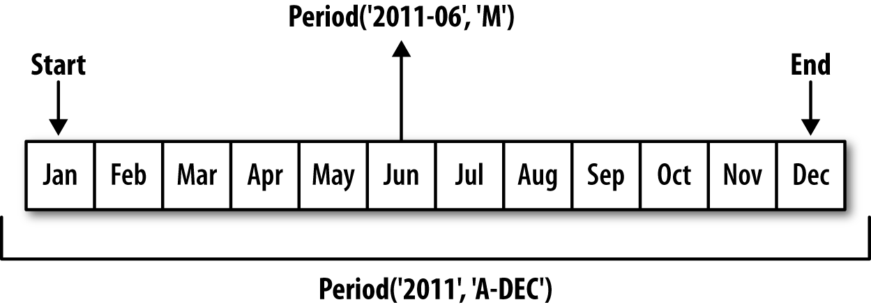
When you are converting from high to low frequency, pandas determines the superperiod depending on where the subperiod “belongs.” For example,
in A-JUN frequency, the month
Aug-2007 is actually part of the
2008 period:
In[168]:p=pd.Period('Aug-2007','M')In[169]:p.asfreq('A-JUN')Out[169]:Period('2008','A-JUN')
Whole PeriodIndex objects or
time series can be similarly converted with the same semantics:
In[170]:rng=pd.period_range('2006','2009',freq='A-DEC')In[171]:ts=pd.Series(np.random.randn(len(rng)),index=rng)In[172]:tsOut[172]:20061.60757820070.2003812008-0.8340682009-0.302988Freq:A-DEC,dtype:float64In[173]:ts.asfreq('M',how='start')Out[173]:2006-011.6075782007-010.2003812008-01-0.8340682009-01-0.302988Freq:M,dtype:float64
Here, the annual periods are replaced with monthly periods
corresponding to the first month falling within each annual period. If
we instead wanted the last business day of each year, we can use the
'B' frequency and indicate that we want the end of
the period:
In[174]:ts.asfreq('B',how='end')Out[174]:2006-12-291.6075782007-12-310.2003812008-12-31-0.8340682009-12-31-0.302988Freq:B,dtype:float64
Quarterly data is standard in accounting, finance, and other fields. Much
quarterly data is reported relative to a fiscal year
end, typically the last calendar or business day of one of
the 12 months of the year. Thus, the period 2012Q4 has a different meaning depending on
fiscal year end. pandas supports all 12 possible quarterly frequencies
as Q-JAN through Q-DEC:
In[175]:p=pd.Period('2012Q4',freq='Q-JAN')In[176]:pOut[176]:Period('2012Q4','Q-JAN')
In the case of fiscal year ending in January, 2012Q4 runs from November through January,
which you can check by converting to daily frequency. See Figure 11-2 for an illustration.
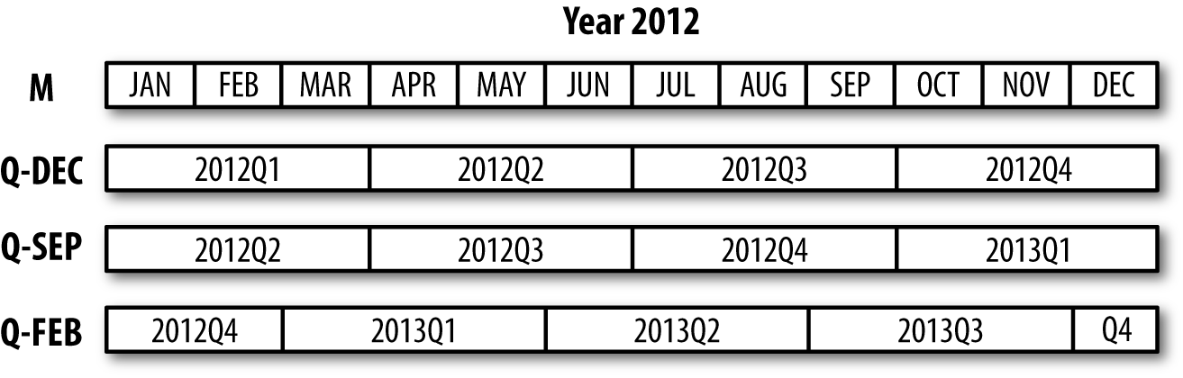
In[177]:p.asfreq('D','start')Out[177]:Period('2011-11-01','D')In[178]:p.asfreq('D','end')Out[178]:Period('2012-01-31','D')
Thus, it’s possible to do easy period arithmetic; for example, to get the timestamp at 4 PM on the second-to-last business day of the quarter, you could do:
In[179]:p4pm=(p.asfreq('B','e')-1).asfreq('T','s')+16*60In[180]:p4pmOut[180]:Period('2012-01-30 16:00','T')In[181]:p4pm.to_timestamp()Out[181]:Timestamp('2012-01-30 16:00:00')
You can generate quarterly ranges using period_range.
Arithmetic is identical, too:
In[182]:rng=pd.period_range('2011Q3','2012Q4',freq='Q-JAN')In[183]:ts=pd.Series(np.arange(len(rng)),index=rng)In[184]:tsOut[184]:2011Q302011Q412012Q122012Q232012Q342012Q45Freq:Q-JAN,dtype:int64In[185]:new_rng=(rng.asfreq('B','e')-1).asfreq('T','s')+16*60In[186]:ts.index=new_rng.to_timestamp()In[187]:tsOut[187]:2010-10-2816:00:0002011-01-2816:00:0012011-04-2816:00:0022011-07-2816:00:0032011-10-2816:00:0042012-01-3016:00:005dtype:int64
Series and DataFrame objects indexed by timestamps can be converted to periods with
the to_period
method:
In[188]:rng=pd.date_range('2000-01-01',periods=3,freq='M')In[189]:ts=pd.Series(np.random.randn(3),index=rng)In[190]:tsOut[190]:2000-01-311.6632612000-02-29-0.9962062000-03-311.521760Freq:M,dtype:float64In[191]:pts=ts.to_period()In[192]:ptsOut[192]:2000-011.6632612000-02-0.9962062000-031.521760Freq:M,dtype:float64
Since periods refer to non-overlapping timespans, a timestamp can
only belong to a single period for a given frequency. While the
frequency of the new PeriodIndex is
inferred from the timestamps by default, you can specify any frequency
you want. There is also no problem with having duplicate periods in the
result:
In[193]:rng=pd.date_range('1/29/2000',periods=6,freq='D')In[194]:ts2=pd.Series(np.random.randn(6),index=rng)In[195]:ts2Out[195]:2000-01-290.2441752000-01-300.4233312000-01-31-0.6540402000-02-012.0891542000-02-02-0.0602202000-02-03-0.167933Freq:D,dtype:float64In[196]:ts2.to_period('M')Out[196]:2000-010.2441752000-010.4233312000-01-0.6540402000-022.0891542000-02-0.0602202000-02-0.167933Freq:M,dtype:float64
To convert back to timestamps, use to_timestamp:
In[197]:pts=ts2.to_period()In[198]:ptsOut[198]:2000-01-290.2441752000-01-300.4233312000-01-31-0.6540402000-02-012.0891542000-02-02-0.0602202000-02-03-0.167933Freq:D,dtype:float64In[199]:pts.to_timestamp(how='end')Out[199]:2000-01-290.2441752000-01-300.4233312000-01-31-0.6540402000-02-012.0891542000-02-02-0.0602202000-02-03-0.167933Freq:D,dtype:float64
Fixed frequency datasets are sometimes stored with timespan information spread across multiple columns. For example, in this macroeconomic dataset, the year and quarter are in different columns:
In[200]:data=pd.read_csv('examples/macrodata.csv')In[201]:data.head(5)Out[201]:yearquarterrealgdprealconsrealinvrealgovtrealdpicpi\01959.01.02710.3491707.4286.898470.0451886.928.9811959.02.02778.8011733.7310.859481.3011919.729.1521959.03.02775.4881751.8289.226491.2601916.429.3531959.04.02785.2041753.7299.356484.0521931.329.3741960.01.02847.6991770.5331.722462.1991955.529.54m1tbilrateunemppopinflrealint0139.72.825.8177.1460.000.001141.73.085.1177.8302.340.742140.53.825.3178.6572.741.093140.04.335.6179.3860.274.064139.63.505.2180.0072.311.19In[202]:data.yearOut[202]:01959.011959.021959.031959.041960.051960.061960.071960.081961.091961.0...1932007.01942007.01952007.01962008.01972008.01982008.01992008.02002009.02012009.02022009.0Name:year,Length:203,dtype:float64In[203]:data.quarterOut[203]:01.012.023.034.041.052.063.074.081.092.0...1932.01943.01954.01961.01972.01983.01994.02001.02012.02023.0Name:quarter,Length:203,dtype:float64
By passing these arrays to PeriodIndex with a frequency, you can combine them to form an index for the DataFrame:
In[204]:index=pd.PeriodIndex(year=data.year,quarter=data.quarter,.....:freq='Q-DEC')In[205]:indexOut[205]:PeriodIndex(['1959Q1','1959Q2','1959Q3','1959Q4','1960Q1','1960Q2','1960Q3','1960Q4','1961Q1','1961Q2',...'2007Q2','2007Q3','2007Q4','2008Q1','2008Q2','2008Q3','2008Q4','2009Q1','2009Q2','2009Q3'],dtype='period[Q-DEC]',length=203,freq='Q-DEC')In[206]:data.index=indexIn[207]:data.inflOut[207]:1959Q10.001959Q22.341959Q32.741959Q40.271960Q12.311960Q20.141960Q32.701960Q41.211961Q1-0.401961Q21.47...2007Q22.752007Q33.452007Q46.382008Q12.822008Q28.532008Q3-3.162008Q4-8.792009Q10.942009Q23.372009Q33.56Freq:Q-DEC,Name:infl,Length:203,dtype:float64
Resampling refers to the process of converting a time series from one frequency to
another. Aggregating higher frequency data to lower frequency is
called downsampling, while converting
lower frequency to higher frequency is called upsampling. Not all resampling
falls into either of these categories; for example, converting W-WED (weekly on Wednesday) to W-FRI is neither upsampling nor
downsampling.
pandas objects are equipped with a resample method, which
is the workhorse function for all frequency conversion.
resample has a similar API to
groupby; you call resample to group
the data, then call an aggregation function:
In[208]:rng=pd.date_range('2000-01-01',periods=100,freq='D')In[209]:ts=pd.Series(np.random.randn(len(rng)),index=rng)In[210]:tsOut[210]:2000-01-010.6316342000-01-02-1.5943132000-01-03-1.5199372000-01-041.1087522000-01-051.2558532000-01-06-0.0243302000-01-07-2.0479392000-01-08-0.2726572000-01-09-1.6926152000-01-101.423830...2000-03-31-0.0078522000-04-01-1.6388062000-04-021.4012272000-04-031.7585392000-04-040.6289322000-04-05-0.4237762000-04-060.7897402000-04-070.9375682000-04-08-2.2532942000-04-09-1.772919Freq:D,Length:100,dtype:float64In[211]:ts.resample('M').mean()Out[211]:2000-01-31-0.1658932000-02-290.0786062000-03-310.2238112000-04-30-0.063643Freq:M,dtype:float64In[212]:ts.resample('M',kind='period').mean()Out[212]:2000-01-0.1658932000-020.0786062000-030.2238112000-04-0.063643Freq:M,dtype:float64
resample is a flexible and
high-performance method that can be used to process very large time
series. The examples in the following sections illustrate its semantics
and use. Table 11-5 summarizes some of its
options.
| Argument | Description |
|---|---|
freq | String or DateOffset indicating desired resampled frequency
(e.g., ‘M', ’5min', or Second(15)) |
axis | Axis to resample on; default axis=0 |
fill_method | How to interpolate when upsampling, as in 'ffill' or 'bfill'; by default does no
interpolation |
closed | In downsampling, which end of each interval is closed
(inclusive), 'right' or
'left' |
label | In downsampling, how to label the aggregated result, with
the 'right' or 'left' bin edge (e.g., the 9:30 to 9:35
five-minute interval could be labeled 9:30 or 9:35) |
loffset | Time adjustment to the bin labels, such as '-1s' / Second(-1) to shift the aggregate labels
one second earlier |
limit | When forward or backward filling, the maximum number of periods to fill |
kind | Aggregate to periods ('period') or timestamps ('timestamp'); defaults to the type of
index the time series has |
convention | When resampling periods, the convention ('start' or 'end') for converting the low-frequency
period to high frequency; defaults to 'end' |
Aggregating data to a regular, lower frequency is a pretty normal time series task. The
data you’re aggregating doesn’t need to be fixed frequently; the desired
frequency defines bin edges that are used to slice
the time series into pieces to aggregate. For example, to convert to
monthly, 'M' or 'BM', you need to chop up the data into one-month intervals. Each interval is said to be
half-open; a data point can only belong to one
interval, and the union of the intervals must make up the whole time
frame. There are a couple things to think about when using resample to downsample data:
Which side of each interval is closed
How to label each aggregated bin, either with the start of the interval or the end
To illustrate, let’s look at some one-minute data:
In[213]:rng=pd.date_range('2000-01-01',periods=12,freq='T')In[214]:ts=pd.Series(np.arange(12),index=rng)In[215]:tsOut[215]:2000-01-0100:00:0002000-01-0100:01:0012000-01-0100:02:0022000-01-0100:03:0032000-01-0100:04:0042000-01-0100:05:0052000-01-0100:06:0062000-01-0100:07:0072000-01-0100:08:0082000-01-0100:09:0092000-01-0100:10:00102000-01-0100:11:0011Freq:T,dtype:int64
Suppose you wanted to aggregate this data into five-minute chunks or bars by taking the sum of each group:
In[216]:ts.resample('5min',closed='right').sum()Out[216]:1999-12-3123:55:0002000-01-0100:00:00152000-01-0100:05:00402000-01-0100:10:0011Freq:5T,dtype:int64
The frequency you pass defines bin edges in five-minute
increments. By default, the
left bin edge is inclusive, so the
00:00 value is included in the
00:00 to 00:05 interval.1 Passing closed='right'
changes the interval to be closed on the right:
In[217]:ts.resample('5min',closed='right').sum()Out[217]:1999-12-3123:55:0002000-01-0100:00:00152000-01-0100:05:00402000-01-0100:10:0011Freq:5T,dtype:int64
The resulting time series is labeled by the timestamps from the
left side of each bin. By passing label='right' you can label them with the
right bin edge:
In[218]:ts.resample('5min',closed='right',label='right').sum()Out[218]:2000-01-0100:00:0002000-01-0100:05:00152000-01-0100:10:00402000-01-0100:15:0011Freq:5T,dtype:int64
See Figure 11-3 for an illustration of minute frequency data being resampled to five-minute frequency.
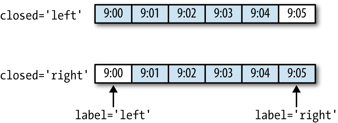
Lastly, you might want to shift the result index by some amount,
say subtracting one second from the right edge to make it more clear
which interval the timestamp refers to. To do this, pass a string or
date offset to loffset:
In[219]:ts.resample('5min',closed='right',.....:label='right',loffset='-1s').sum()Out[219]:1999-12-3123:59:5902000-01-0100:04:59152000-01-0100:09:59402000-01-0100:14:5911Freq:5T,dtype:int64
You also could have accomplished the effect of loffset by calling the shift method on the
result without the loffset.
In finance, a popular way to aggregate a time series is to compute
four values for each bucket: the first (open), last (close), maximum
(high), and minimal (low) values. By using the ohlc
aggregate function you will obtain a DataFrame having columns
containing these four aggregates, which are efficiently computed in a
single sweep of the data:
In[220]:ts.resample('5min').ohlc()Out[220]:openhighlowclose2000-01-0100:00:0004042000-01-0100:05:0059592000-01-0100:10:0010111011
When converting from a low frequency to a higher frequency, no aggregation is needed. Let’s consider a DataFrame with some weekly data:
In[221]:frame=pd.DataFrame(np.random.randn(2,4),.....:index=pd.date_range('1/1/2000',periods=2,.....:freq='W-WED'),.....:columns=['Colorado','Texas','New York','Ohio'])In[222]:frameOut[222]:ColoradoTexasNewYorkOhio2000-01-05-0.8964310.6772630.0365030.0871022000-01-12-0.0466620.9272380.482284-0.867130
When you are using an aggregation function with this data, there is only
one value per group, and missing values result in the gaps. We use the
asfreq method to convert to the higher frequency without any
aggregation:
In[223]:df_daily=frame.resample('D').asfreq()In[224]:df_dailyOut[224]:ColoradoTexasNewYorkOhio2000-01-05-0.8964310.6772630.0365030.0871022000-01-06NaNNaNNaNNaN2000-01-07NaNNaNNaNNaN2000-01-08NaNNaNNaNNaN2000-01-09NaNNaNNaNNaN2000-01-10NaNNaNNaNNaN2000-01-11NaNNaNNaNNaN2000-01-12-0.0466620.9272380.482284-0.867130
Suppose you wanted to fill forward each weekly value on the
non-Wednesdays. The same filling or interpolation methods available in the fillna
and reindex methods are available for
resampling:
In[225]:frame.resample('D').ffill()Out[225]:ColoradoTexasNewYorkOhio2000-01-05-0.8964310.6772630.0365030.0871022000-01-06-0.8964310.6772630.0365030.0871022000-01-07-0.8964310.6772630.0365030.0871022000-01-08-0.8964310.6772630.0365030.0871022000-01-09-0.8964310.6772630.0365030.0871022000-01-10-0.8964310.6772630.0365030.0871022000-01-11-0.8964310.6772630.0365030.0871022000-01-12-0.0466620.9272380.482284-0.867130
You can similarly choose to only fill a certain number of periods forward to limit how far to continue using an observed value:
In[226]:frame.resample('D').ffill(limit=2)Out[226]:ColoradoTexasNewYorkOhio2000-01-05-0.8964310.6772630.0365030.0871022000-01-06-0.8964310.6772630.0365030.0871022000-01-07-0.8964310.6772630.0365030.0871022000-01-08NaNNaNNaNNaN2000-01-09NaNNaNNaNNaN2000-01-10NaNNaNNaNNaN2000-01-11NaNNaNNaNNaN2000-01-12-0.0466620.9272380.482284-0.867130
Notably, the new date index need not overlap with the old one at all:
In[227]:frame.resample('W-THU').ffill()Out[227]:ColoradoTexasNewYorkOhio2000-01-06-0.8964310.6772630.0365030.0871022000-01-13-0.0466620.9272380.482284-0.867130
Resampling data indexed by periods is similar to timestamps:
In[228]:frame=pd.DataFrame(np.random.randn(24,4),.....:index=pd.period_range('1-2000','12-2001',.....:freq='M'),.....:columns=['Colorado','Texas','New York','Ohio'])In[229]:frame[:5]Out[229]:ColoradoTexasNewYorkOhio2000-010.493841-0.1554341.3972861.5070552000-02-1.1794420.4431711.395676-0.5296582000-030.7873580.2488450.7432391.2677462000-041.302395-0.272154-0.051532-0.4677402000-05-1.0408160.4264190.312945-1.115689In[230]:annual_frame=frame.resample('A-DEC').mean()In[231]:annual_frameOut[231]:ColoradoTexasNewYorkOhio20000.5567030.0166310.111873-0.02744520010.0463030.1633440.251503-0.157276
Upsampling is more nuanced, as you must make a decision about which
end of the timespan in the new frequency to place the values before
resampling, just like the asfreq
method. The convention argument
defaults to 'start' but can also be
'end':
# Q-DEC: Quarterly, year ending in DecemberIn[232]:annual_frame.resample('Q-DEC').ffill()Out[232]:ColoradoTexasNewYorkOhio2000Q10.5567030.0166310.111873-0.0274452000Q20.5567030.0166310.111873-0.0274452000Q30.5567030.0166310.111873-0.0274452000Q40.5567030.0166310.111873-0.0274452001Q10.0463030.1633440.251503-0.1572762001Q20.0463030.1633440.251503-0.1572762001Q30.0463030.1633440.251503-0.1572762001Q40.0463030.1633440.251503-0.157276In[233]:annual_frame.resample('Q-DEC',convention='end').ffill()Out[233]:ColoradoTexasNewYorkOhio2000Q40.5567030.0166310.111873-0.0274452001Q10.5567030.0166310.111873-0.0274452001Q20.5567030.0166310.111873-0.0274452001Q30.5567030.0166310.111873-0.0274452001Q40.0463030.1633440.251503-0.157276
Since periods refer to timespans, the rules about upsampling and downsampling are more rigid:
In downsampling, the target frequency must be a subperiod of the source frequency.
In upsampling, the target frequency must be a superperiod of the source frequency.
If these rules are not satisfied, an exception will be raised.
This mainly affects the quarterly, annual, and weekly frequencies; for
example, the timespans defined by Q-MAR only line up with A-MAR, A-JUN, A-SEP, and A-DEC:
In[234]:annual_frame.resample('Q-MAR').ffill()Out[234]:ColoradoTexasNewYorkOhio2000Q40.5567030.0166310.111873-0.0274452001Q10.5567030.0166310.111873-0.0274452001Q20.5567030.0166310.111873-0.0274452001Q30.5567030.0166310.111873-0.0274452001Q40.0463030.1633440.251503-0.1572762002Q10.0463030.1633440.251503-0.1572762002Q20.0463030.1633440.251503-0.1572762002Q30.0463030.1633440.251503-0.157276
An important class of array transformations used for time series operations are statistics and other functions evaluated over a sliding window or with exponentially decaying weights. This can be useful for smoothing noisy or gappy data. I call these moving window functions, even though it includes functions without a fixed-length window like exponentially weighted moving average. Like other statistical functions, these also automatically exclude missing data.
Before digging in, we can load up some time series data and resample it to business day frequency:
In[235]:close_px_all=pd.read_csv('examples/stock_px_2.csv',.....:parse_dates=True,index_col=0)In[236]:close_px=close_px_all[['AAPL','MSFT','XOM']]In[237]:close_px=close_px.resample('B').ffill()
I now introduce the rolling operator, which behaves similarly to resample and
groupby. It can be called on a Series or DataFrame
along with a window (expressed as a
number of periods; see Figure 11-4 for the plot
created):
In[238]:close_px.AAPL.plot()Out[238]:<matplotlib.axes._subplots.AxesSubplotat0x7fa59eaf0b00>In[239]:close_px.AAPL.rolling(250).mean().plot()
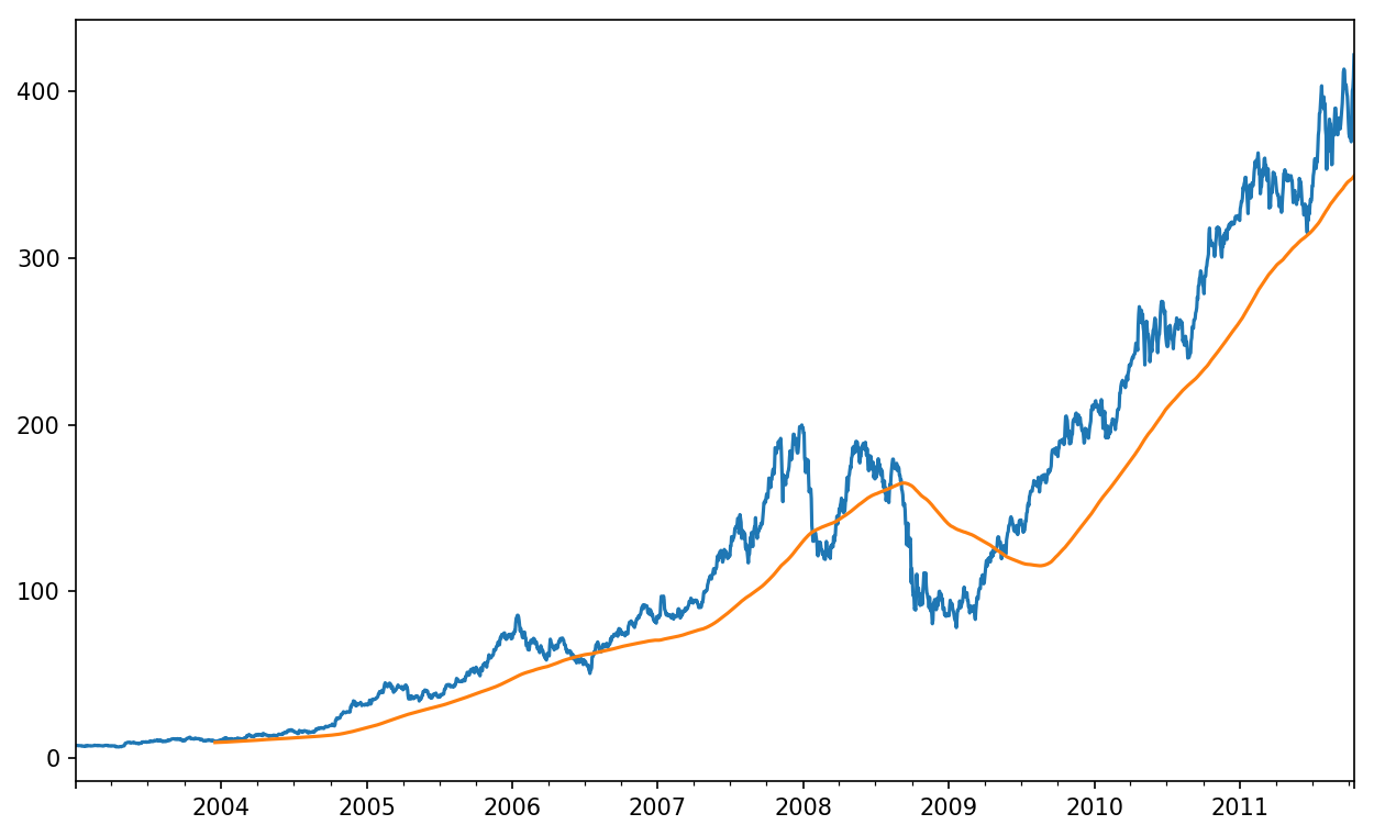
The expression rolling(250) is similar in
behavior to groupby, but instead of grouping it creates
an object that enables grouping over a 250-day sliding window. So here we
have the 250-day moving window average of Apple’s stock price.
By default rolling functions require all of the values in the window
to be non-NA. This behavior can be changed to account for missing data
and, in particular, the fact that you will have fewer than window periods of data at the beginning of the
time series (see Figure 11-5):
In[241]:appl_std250=close_px.AAPL.rolling(250,min_periods=10).std()In[242]:appl_std250[5:12]Out[242]:2003-01-09NaN2003-01-10NaN2003-01-13NaN2003-01-14NaN2003-01-150.0774962003-01-160.0747602003-01-170.112368Freq:B,Name:AAPL,dtype:float64In[243]:appl_std250.plot()
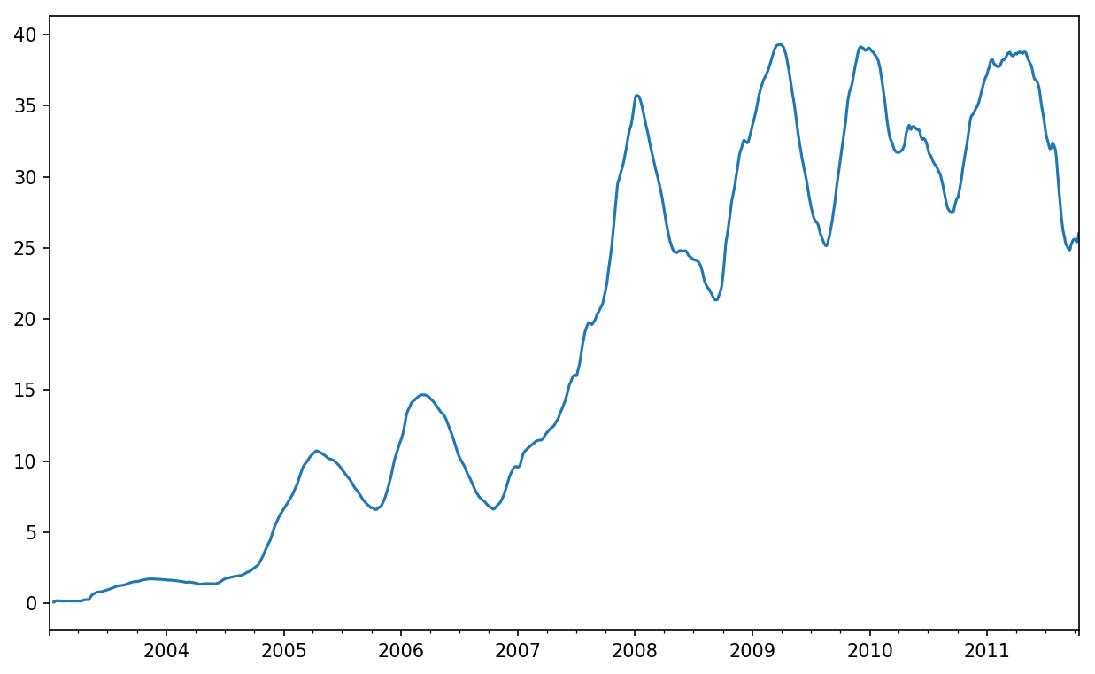
In order to compute an expanding window mean,
use the expanding operator instead of
rolling. The expanding mean starts the time window from
the beginning of the time series and increases the size of the window
until it encompasses the whole series. An expanding window mean on the
apple_std250 time series looks like this:
In[244]:expanding_mean=appl_std250.expanding().mean()
Calling a moving window function on a DataFrame applies the transformation to each column (see Figure 11-6):
In[246]:close_px.rolling(60).mean().plot(logy=True)
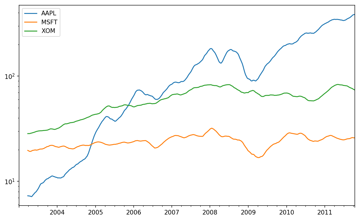
The rolling function also accepts a string indicating a fixed-size time offset
rather than a set number of periods. Using this notation can be useful for
irregular time series. These are the same strings that you can pass to
resample. For example, we could compute a 20-day
rolling mean like so:
In[247]:close_px.rolling('20D').mean()Out[247]:AAPLMSFTXOM2003-01-027.40000021.11000029.2200002003-01-037.42500021.12500029.2300002003-01-067.43333321.25666729.4733332003-01-077.43250021.42500029.3425002003-01-087.40200021.40200029.2400002003-01-097.39166721.49000029.2733332003-01-107.38714321.55857129.2385712003-01-137.37875021.63375029.1975002003-01-147.37000021.71777829.1944442003-01-157.35500021.75700029.152000............2011-10-03398.00214325.89071472.4135712011-10-04396.80214325.80785772.4271432011-10-05395.75142925.72928672.4228572011-10-06394.09928625.67357172.3757142011-10-07392.47933325.71200072.4546672011-10-10389.35142925.60214372.5278572011-10-11388.50500025.67428672.8350002011-10-12388.53142925.81000073.4007142011-10-13388.82642925.96142973.9050002011-10-14391.03800026.04866774.185333[2292rowsx3columns]
An alternative to using a static window size with equally weighted observations is to specify a constant decay factor to give more weight to more recent observations. There are a couple of ways to specify the decay factor. A popular one is using a span, which makes the result comparable to a simple moving window function with window size equal to the span.
Since an exponentially weighted statistic places more weight on more recent observations, it “adapts” faster to changes compared with the equal-weighted version.
pandas has the ewm operator to go along with rolling and
expanding. Here’s an example comparing a 60-day
moving average of Apple’s stock price with an EW moving average with
span=60 (see Figure 11-7):
In[249]:aapl_px=close_px.AAPL['2006':'2007']In[250]:ma60=aapl_px.rolling(30,min_periods=20).mean()In[251]:ewma60=aapl_px.ewm(span=30).mean()In[252]:ma60.plot(style='k--',label='Simple MA')Out[252]:<matplotlib.axes._subplots.AxesSubplotat0x7fa59e5df908>In[253]:ewma60.plot(style='k-',label='EW MA')Out[253]:<matplotlib.axes._subplots.AxesSubplotat0x7fa59e5df908>In[254]:plt.legend()
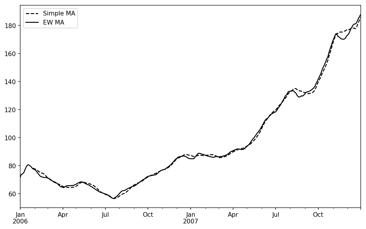
Some statistical operators, like correlation and covariance, need to operate on two time series. As an example, financial analysts are often interested in a stock’s correlation to a benchmark index like the S&P 500. To have a look at this, we first compute the percent change for all of our time series of interest:
In[256]:spx_px=close_px_all['SPX']In[257]:spx_rets=spx_px.pct_change()In[258]:returns=close_px.pct_change()
The corr aggregation function after we call rolling can then compute
the rolling correlation with spx_rets (see Figure 11-8 for the resulting plot):
In[259]:corr=returns.AAPL.rolling(125,min_periods=100).corr(spx_rets)In[260]:corr.plot()
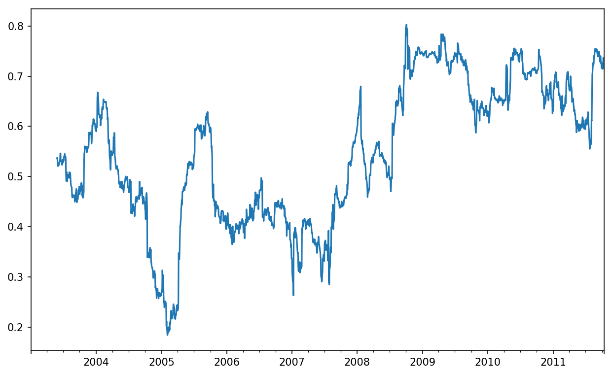
Suppose you wanted to compute the correlation of the S&P 500
index with many stocks at once. Writing a loop and creating a new
DataFrame would be easy but might get repetitive, so if you pass a
Series and a DataFrame, a function like rolling_corr will
compute the correlation of the Series (spx_rets, in this case) with each column in
the DataFrame (see Figure 11-9 for the plot of
the result):
In[262]:corr=returns.rolling(125,min_periods=100).corr(spx_rets)In[263]:corr.plot()
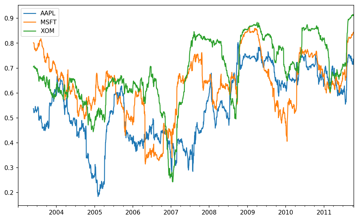
The apply method on
rolling and related methods provides a means to apply an array
function of your own devising over a moving window. The only requirement
is that the function produce a single value (a reduction) from each
piece of the array. For example, while we can compute sample quantiles
using rolling(...).quantile(q), we
might be interested in the percentile rank of a particular value over
the sample. The scipy.stats.percentileofscore function
does just this (see Figure 11-10 for
the resulting plot):
In[265]:fromscipy.statsimportpercentileofscoreIn[266]:score_at_2percent=lambdax:percentileofscore(x,0.02)In[267]:result=returns.AAPL.rolling(250).apply(score_at_2percent)In[268]:result.plot()
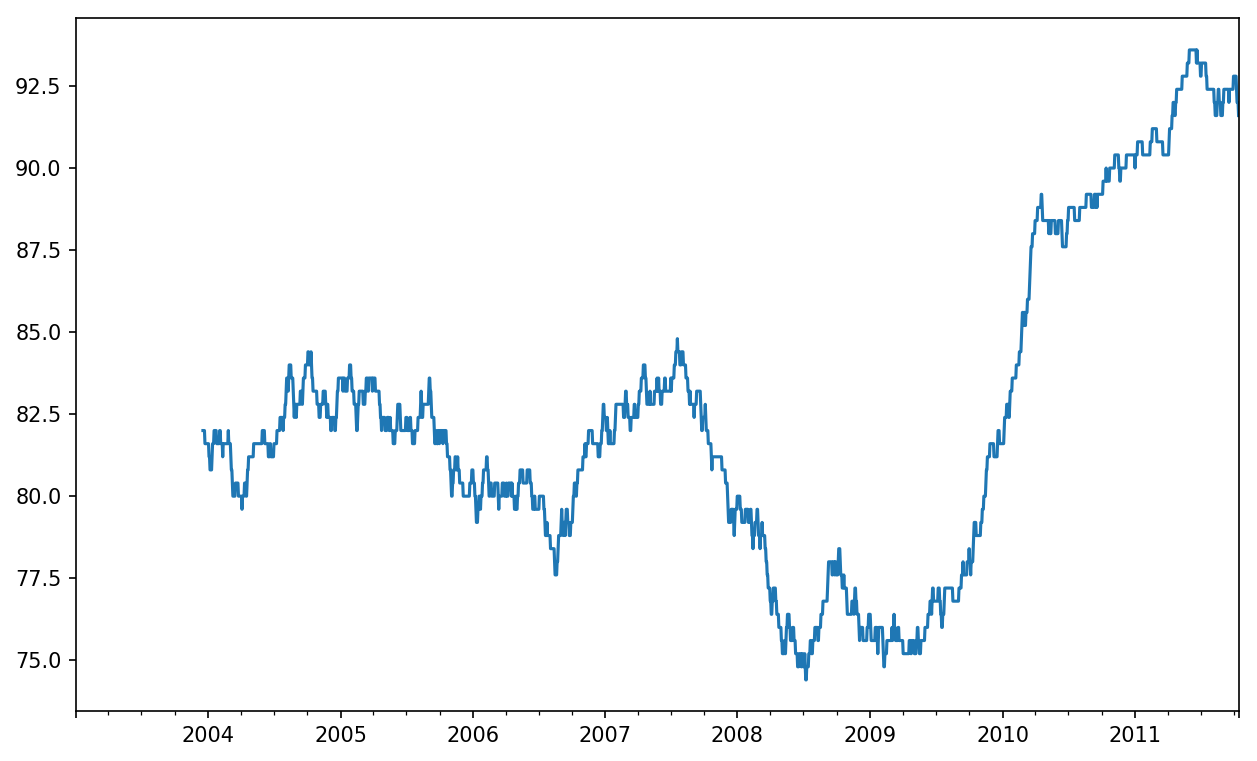
If you don’t have SciPy installed already, you can install it with conda or pip.
Time series data calls for different types of analysis and data transformation tools than the other types of data we have explored in previous chapters.
In the following chapters, we will move on to some advanced pandas methods and show how to start using modeling libraries like statsmodels and scikit-learn.
1 The choice of the default values for closed and label might seem a bit odd to some users.
In practice the choice is somewhat arbitrary; for some target
frequencies, closed='left' is
preferable, while for others closed='right' makes more sense. The
important thing is that you keep in mind exactly how you are
segmenting the data.
The preceding chapters have focused on introducing different types of data wrangling workflows and features of NumPy, pandas, and other libraries. Over time, pandas has developed a depth of features for power users. This chapter digs into a few more advanced feature areas to help you deepen your expertise as a pandas user.
This section introduces the pandas Categorical type. I will show how
you can achieve better performance and memory use in some pandas
operations by using it. I also introduce some tools for using categorical
data in statistics and machine learning applications.
Frequently, a column in a table may contain repeated instances of
a smaller set of distinct values. We have already seen functions
like unique and
value_counts, which enable us to extract the distinct
values from an array and compute their frequencies, respectively:
In[10]:importnumpyasnp;importpandasaspdIn[11]:values=pd.Series(['apple','orange','apple',....:'apple']*2)In[12]:valuesOut[12]:0apple1orange2apple3apple4apple5orange6apple7appledtype:objectIn[13]:pd.unique(values)Out[13]:array(['apple','orange'],dtype=object)In[14]:pd.value_counts(values)Out[14]:apple6orange2dtype:int64
Many data systems (for data warehousing, statistical computing, or other uses) have developed specialized approaches for representing data with repeated values for more efficient storage and computation. In data warehousing, a best practice is to use so-called dimension tables containing the distinct values and storing the primary observations as integer keys referencing the dimension table:
In[15]:values=pd.Series([0,1,0,0]*2)In[16]:dim=pd.Series(['apple','orange'])In[17]:valuesOut[17]:0011203040516070dtype:int64In[18]:dimOut[18]:0apple1orangedtype:object
We can use the take method to restore the original Series of strings:
In[19]:dim.take(values)Out[19]:0apple1orange0apple0apple0apple1orange0apple0appledtype:object
This representation as integers is called the categorical or dictionary-encoded representation. The array of distinct values can be called the categories, dictionary, or levels of the data. In this book we will use the terms categorical and categories. The integer values that reference the categories are called the category codes or simply codes.
The categorical representation can yield significant performance improvements when you are doing analytics. You can also perform transformations on the categories while leaving the codes unmodified. Some example transformations that can be made at relatively low cost are:
Renaming categories
Appending a new category without changing the order or position of the existing categories
pandas has a special Categorical type for
holding data that uses the integer-based categorical representation or
encoding. Let’s consider the example Series from
before:
In[20]:fruits=['apple','orange','apple','apple']*2In[21]:N=len(fruits)In[22]:df=pd.DataFrame({'fruit':fruits,....:'basket_id':np.arange(N),....:'count':np.random.randint(3,15,size=N),....:'weight':np.random.uniform(0,4,size=N)},....:columns=['basket_id','fruit','count','weight'])In[23]:dfOut[23]:basket_idfruitcountweight00apple53.85805811orange82.61270822apple42.99562733apple72.61427944apple122.99085955orange83.84522766apple50.03355377apple40.425778
Here, df['fruit'] is an array of Python string
objects. We can convert it to categorical by calling:
In[24]:fruit_cat=df['fruit'].astype('category')In[25]:fruit_catOut[25]:0apple1orange2apple3apple4apple5orange6apple7appleName:fruit,dtype:categoryCategories(2,object):[apple,orange]
The values for fruit_cat are not a NumPy array,
but an instance of pandas.Categorical:
In[26]:c=fruit_cat.valuesIn[27]:type(c)Out[27]:pandas.core.categorical.Categorical
The Categorical object has
categories and codes
attributes:
In[28]:c.categoriesOut[28]:Index(['apple','orange'],dtype='object')In[29]:c.codesOut[29]:array([0,1,0,0,0,1,0,0],dtype=int8)
You can convert a DataFrame column to categorical by assigning the converted result:
In[30]:df['fruit']=df['fruit'].astype('category')In[31]:df.fruitOut[31]:0apple1orange2apple3apple4apple5orange6apple7appleName:fruit,dtype:categoryCategories(2,object):[apple,orange]
You can also create pandas.Categorical directly
from other types of Python sequences:
In[32]:my_categories=pd.Categorical(['foo','bar','baz','foo','bar'])In[33]:my_categoriesOut[33]:[foo,bar,baz,foo,bar]Categories(3,object):[bar,baz,foo]
If you have obtained categorical encoded data from another source,
you can use the alternative from_codes
constructor:
In[34]:categories=['foo','bar','baz']In[35]:codes=[0,1,2,0,0,1]In[36]:my_cats_2=pd.Categorical.from_codes(codes,categories)In[37]:my_cats_2Out[37]:[foo,bar,baz,foo,foo,bar]Categories(3,object):[foo,bar,baz]
Unless explicitly specified, categorical conversions assume no
specific ordering of the categories. So the
categories array may be in a different order
depending on the ordering of the input data. When using
from_codes or any of the other constructors, you can
indicate that the categories have a meaningful ordering:
In[38]:ordered_cat=pd.Categorical.from_codes(codes,categories,....:ordered=True)In[39]:ordered_catOut[39]:[foo,bar,baz,foo,foo,bar]Categories(3,object):[foo<bar<baz]
The output [foo < bar < baz] indicates
that 'foo' precedes 'bar' in the
ordering, and so on. An unordered categorical instance can be made
ordered with as_ordered:
In[40]:my_cats_2.as_ordered()Out[40]:[foo,bar,baz,foo,foo,bar]Categories(3,object):[foo<bar<baz]
As a last note, categorical data need not be strings, even though I have only showed string examples. A categorical array can consist of any immutable value types.
Using Categorical in pandas compared with the non-encoded version
(like an array of strings) generally behaves the same way. Some parts of
pandas, like the groupby function, perform better
when working with categoricals. There are also some
functions that can utilize the ordered flag.
Let’s consider some random numeric data, and use the pandas.qcut binning function. This
return pandas.Categorical; we used
pandas.cut earlier in the book but glossed over the
details of how categoricals work:
In[41]:np.random.seed(12345)In[42]:draws=np.random.randn(1000)In[43]:draws[:5]Out[43]:array([-0.2047,0.4789,-0.5194,-0.5557,1.9658])
Let’s compute a quartile binning of this data and extract some statistics:
In[44]:bins=pd.qcut(draws,4)In[45]:binsOut[45]:[(-0.684,-0.0101],(-0.0101,0.63],(-0.684,-0.0101],(-0.684,-0.0101],(0.63,3.928],...,(-0.0101,0.63],(-0.684,-0.0101],(-2.95,-0.684],(-0.0101,0.63],(0.63,3.928]]Length:1000Categories(4,interval[float64]):[(-2.95,-0.684]<(-0.684,-0.0101]<(-0.0101,0.63]<(0.63,3.928]]
While useful, the exact sample quartiles may be less useful for
producing a report than quartile names. We can achieve this with the
labels argument to qcut:
In[46]:bins=pd.qcut(draws,4,labels=['Q1','Q2','Q3','Q4'])In[47]:binsOut[47]:[Q2,Q3,Q2,Q2,Q4,...,Q3,Q2,Q1,Q3,Q4]Length:1000Categories(4,object):[Q1<Q2<Q3<Q4]In[48]:bins.codes[:10]Out[48]:array([1,2,1,1,3,3,2,2,3,3],dtype=int8)
The labeled bins categorical does not contain
information about the bin edges in the data, so we can use
groupby to extract some summary statistics:
In[49]:bins=pd.Series(bins,name='quartile')In[50]:results=(pd.Series(draws)....:.groupby(bins)....:.agg(['count','min','max'])....:.reset_index())In[51]:resultsOut[51]:quartilecountminmax0Q1250-2.949343-0.6854841Q2250-0.683066-0.0101152Q3250-0.0100320.6288943Q42500.6342383.927528
The 'quartile' column in the result retains the
original categorical information, including ordering, from
bins:
In[52]:results['quartile']Out[52]:0Q11Q22Q33Q4Name:quartile,dtype:categoryCategories(4,object):[Q1<Q2<Q3<Q4]
If you do a lot of analytics on a particular dataset, converting to categorical can yield substantial overall performance gains. A categorical version of a DataFrame column will often use significantly less memory, too. Let’s consider some Series with 10 million elements and a small number of distinct categories:
In[53]:N=10000000In[54]:draws=pd.Series(np.random.randn(N))In[55]:labels=pd.Series(['foo','bar','baz','qux']*(N//4))
Now we convert labels to categorical:
In[56]:categories=labels.astype('category')
Now we note that labels uses significantly
more memory than categories:
In[57]:labels.memory_usage()Out[57]:80000080In[58]:categories.memory_usage()Out[58]:10000272
The conversion to category is not free, of course, but it is a one-time cost:
In[59]:%time_=labels.astype('category')CPUtimes:user360ms,sys:140ms,total:500msWalltime:502ms
GroupBy operations can be significantly faster with categoricals because the underlying algorithms use the integer-based codes array instead of an array of strings.
Series containing categorical data have several special methods similar to the
Series.str specialized string methods. This also
provides convenient access to the categories and codes. Consider the
Series:
In[60]:s=pd.Series(['a','b','c','d']*2)In[61]:cat_s=s.astype('category')In[62]:cat_sOut[62]:0a1b2c3d4a5b6c7ddtype:categoryCategories(4,object):[a,b,c,d]
The special attribute cat provides access to
categorical methods:
In[63]:cat_s.cat.codesOut[63]:0011223340516273dtype:int8In[64]:cat_s.cat.categoriesOut[64]:Index(['a','b','c','d'],dtype='object')
Suppose that we know the actual set of categories for this data
extends beyond the four values observed in the data. We can use the
set_categories method to change them:
In[65]:actual_categories=['a','b','c','d','e']In[66]:cat_s2=cat_s.cat.set_categories(actual_categories)In[67]:cat_s2Out[67]:0a1b2c3d4a5b6c7ddtype:categoryCategories(5,object):[a,b,c,d,e]
While it appears that the data is unchanged, the new categories
will be reflected in operations that use them. For example,
value_counts respects the categories, if
present:
In[68]:cat_s.value_counts()Out[68]:d2c2b2a2dtype:int64In[69]:cat_s2.value_counts()Out[69]:d2c2b2a2e0dtype:int64
In large datasets, categoricals are often used as a convenient
tool for memory savings and better performance. After you filter a large
DataFrame or Series, many of the categories may not appear in the data.
To help with this, we can use the
remove_unused_categories method to trim unobserved
categories:
In[70]:cat_s3=cat_s[cat_s.isin(['a','b'])]In[71]:cat_s3Out[71]:0a1b4a5bdtype:categoryCategories(4,object):[a,b,c,d]In[72]:cat_s3.cat.remove_unused_categories()Out[72]:0a1b4a5bdtype:categoryCategories(2,object):[a,b]
See Table 12-1 for a listing of available categorical methods.
When you’re using statistics or machine learning tools, you’ll often transform categorical data into dummy variables, also known as one-hot encoding. This involves creating a DataFrame with a column for each distinct category; these columns contain 1s for occurrences of a given category and 0 otherwise.
Consider the previous example:
In[73]:cat_s=pd.Series(['a','b','c','d']*2,dtype='category')
As mentioned previously in Chapter 7,
the pandas.get_dummies function converts this one-dimensional categorical data into a
DataFrame containing the dummy variable:
In[74]:pd.get_dummies(cat_s)Out[74]:abcd0100010100200103000141000501006001070001
While we’ve already discussed using the groupby method for
Series and DataFrame in depth in Chapter 10, there are
some additional techniques that you may find of use.
In Chapter 10 we looked at the apply method in grouped operations
for performing transformations. There is another built-in method
called transform, which is similar to
apply but imposes more constraints on the kind of
function you can use:
It can produce a scalar value to be broadcast to the shape of the group
It can produce an object of the same shape as the input group
It must not mutate its input
Let’s consider a simple example for illustration:
In[75]:df=pd.DataFrame({'key':['a','b','c']*4,....:'value':np.arange(12.)})In[76]:dfOut[76]:keyvalue0a0.01b1.02c2.03a3.04b4.05c5.06a6.07b7.08c8.09a9.010b10.011c11.0
Here are the group means by key:
In[77]:g=df.groupby('key').valueIn[78]:g.mean()Out[78]:keya4.5b5.5c6.5Name:value,dtype:float64
Suppose instead we wanted to produce a Series of the same shape as
df['value'] but with values replaced by the average
grouped by 'key'. We can pass the function
lambda x: x.mean() to
transform:
In[79]:g.transform(lambdax:x.mean())Out[79]:04.515.526.534.545.556.564.575.586.594.5105.5116.5Name:value,dtype:float64
For built-in aggregation functions, we can pass a string alias as
with the GroupBy agg method:
In[80]:g.transform('mean')Out[80]:04.515.526.534.545.556.564.575.586.594.5105.5116.5Name:value,dtype:float64
Like apply, transform works
with functions that return Series, but the result must be the same size
as the input. For example, we can multiply each group by 2 using a
lambda function:
In[81]:g.transform(lambdax:x*2)Out[81]:00.012.024.036.048.0510.0612.0714.0816.0918.01020.01122.0Name:value,dtype:float64
As a more complicated example, we can compute the ranks in descending order for each group:
In[82]:g.transform(lambdax:x.rank(ascending=False))Out[82]:04.014.024.033.043.053.062.072.082.091.0101.0111.0Name:value,dtype:float64
Consider a group transformation function composed from simple aggregations:
defnormalize(x):return(x-x.mean())/x.std()
We can obtain equivalent results in this case either using
transform or apply:
In[84]:g.transform(normalize)Out[84]:0-1.1618951-1.1618952-1.1618953-0.3872984-0.3872985-0.38729860.38729870.38729880.38729891.161895101.161895111.161895Name:value,dtype:float64In[85]:g.apply(normalize)Out[85]:0-1.1618951-1.1618952-1.1618953-0.3872984-0.3872985-0.38729860.38729870.38729880.38729891.161895101.161895111.161895Name:value,dtype:float64
Built-in aggregate functions like 'mean' or
'sum' are often much faster than a general
apply function. These also have a “fast past” when
used with transform. This allows us to perform a
so-called unwrapped group operation:
In[86]:g.transform('mean')Out[86]:04.515.526.534.545.556.564.575.586.594.5105.5116.5Name:value,dtype:float64In[87]:normalized=(df['value']-g.transform('mean'))/g.transform('std')In[88]:normalizedOut[88]:0-1.1618951-1.1618952-1.1618953-0.3872984-0.3872985-0.38729860.38729870.38729880.38729891.161895101.161895111.161895Name:value,dtype:float64
While an unwrapped group operation may involve multiple group aggregations, the overall benefit of vectorized operations often outweighs this.
For time series data, the resample method is semantically a
group operation based on a time intervalization. Here’s a small example
table:
In[89]:N=15In[90]:times=pd.date_range('2017-05-20 00:00',freq='1min',periods=N)In[91]:df=pd.DataFrame({'time':times,....:'value':np.arange(N)})In[92]:dfOut[92]:timevalue02017-05-2000:00:00012017-05-2000:01:00122017-05-2000:02:00232017-05-2000:03:00342017-05-2000:04:00452017-05-2000:05:00562017-05-2000:06:00672017-05-2000:07:00782017-05-2000:08:00892017-05-2000:09:009102017-05-2000:10:0010112017-05-2000:11:0011122017-05-2000:12:0012132017-05-2000:13:0013142017-05-2000:14:0014
Here, we can index by 'time' and then
resample:
In[93]:df.set_index('time').resample('5min').count()Out[93]:valuetime2017-05-2000:00:0052017-05-2000:05:0052017-05-2000:10:005
Suppose that a DataFrame contains multiple time series, marked by an additional group key column:
In[94]:df2=pd.DataFrame({'time':times.repeat(3),....:'key':np.tile(['a','b','c'],N),....:'value':np.arange(N*3.)})In[95]:df2[:7]Out[95]:keytimevalue0a2017-05-2000:00:000.01b2017-05-2000:00:001.02c2017-05-2000:00:002.03a2017-05-2000:01:003.04b2017-05-2000:01:004.05c2017-05-2000:01:005.06a2017-05-2000:02:006.0
To do the same resampling for each value of
'key', we introduce the pandas.TimeGrouper object:
In[96]:time_key=pd.TimeGrouper('5min')
We can then set the time index, group by 'key'
and time_key, and aggregate:
In[97]:resampled=(df2.set_index('time')....:.groupby(['key',time_key])....:.sum())In[98]:resampledOut[98]:valuekeytimea2017-05-2000:00:0030.02017-05-2000:05:00105.02017-05-2000:10:00180.0b2017-05-2000:00:0035.02017-05-2000:05:00110.02017-05-2000:10:00185.0c2017-05-2000:00:0040.02017-05-2000:05:00115.02017-05-2000:10:00190.0In[99]:resampled.reset_index()Out[99]:keytimevalue0a2017-05-2000:00:0030.01a2017-05-2000:05:00105.02a2017-05-2000:10:00180.03b2017-05-2000:00:0035.04b2017-05-2000:05:00110.05b2017-05-2000:10:00185.06c2017-05-2000:00:0040.07c2017-05-2000:05:00115.08c2017-05-2000:10:00190.0
One constraint with using TimeGrouper is that
the time must be the index of the Series or DataFrame.
When applying a sequence of transformations to a dataset, you may find yourself creating numerous temporary variables that are never used in your analysis. Consider this example, for instance:
df=load_data()df2=df[df['col2']<0]df2['col1_demeaned']=df2['col1']-df2['col1'].mean()result=df2.groupby('key').col1_demeaned.std()
While we’re not using any real data here, this example highlights
some new methods. First, the DataFrame.assign method
is a functional alternative to column
assignments of the form df[k] = v. Rather than
modifying the object in-place, it returns a new DataFrame with the
indicated modifications. So these statements are equivalent:
# Usual non-functional waydf2=df.copy()df2['k']=v# Functional assign waydf2=df.assign(k=v)
Assigning in-place may execute faster than using
assign, but assign enables easier
method chaining:
result=(df2.assign(col1_demeaned=df2.col1-df2.col2.mean()).groupby('key').col1_demeaned.std())
I used the outer parentheses to make it more convenient to add line breaks.
One thing to keep in mind when doing method chaining is that you may
need to refer to temporary objects. In the preceding example, we cannot
refer to the result of load_data until it has been
assigned to the temporary variable df. To help with
this, assign and many other pandas functions accept
function-like arguments, also known as
callables.
To show callables in action, consider a fragment of the example from before:
df=load_data()df2=df[df['col2']<0]
This can be rewritten as:
df=(load_data()[lambdax:x['col2']<0])
Here, the result of load_data is not assigned to
a variable, so the function passed into [] is then
bound to the object at that stage of the method
chain.
We can continue, then, and write the entire sequence as a single chained expression:
result=(load_data()[lambdax:x.col2<0].assign(col1_demeaned=lambdax:x.col1-x.col1.mean()).groupby('key').col1_demeaned.std())
Whether you prefer to write code in this style is a matter of taste, and splitting up the expression into multiple steps may make your code more readable.
You can accomplish a lot with built-in pandas functions and the approaches to
method chaining with callables that we just looked at. However,
sometimes you need to use your own functions or functions from
third-party libraries. This is where the pipe method
comes in.
Consider a sequence of function calls:
a=f(df,arg1=v1)b=g(a,v2,arg3=v3)c=h(b,arg4=v4)
When using functions that accept and return Series or DataFrame
objects, you can rewrite this using calls to
pipe:
result=(df.pipe(f,arg1=v1).pipe(g,v2,arg3=v3).pipe(h,arg4=v4))
The statement f(df) and
df.pipe(f) are equivalent, but
pipe makes chained invocation easier.
A potentially useful pattern for pipe is to
generalize sequences of operations into reusable functions. As an
example, let’s consider substracting group means from a column:
g=df.groupby(['key1','key2'])df['col1']=df['col1']-g.transform('mean')
Suppose that you wanted to be able to demean more than one column and easily change the group keys. Additionally, you might want to perform this transformation in a method chain. Here is an example implementation:
defgroup_demean(df,by,cols):result=df.copy()g=df.groupby(by)forcincols:result[c]=df[c]-g[c].transform('mean')returnresult
result=(df[df.col1<0].pipe(group_demean,['key1','key2'],['col1']))
pandas, like many open source software projects, is still changing and acquiring new and improved functionality. As elsewhere in this book, the focus here has been on the most stable functionality that is less likely to change over the next several years.
To deepen your expertise as a pandas user, I encourage you to explore the documentation and read the release notes as the development team makes new open source releases. We also invite you to join in on pandas development: fixing bugs, building new features, and improving the documentation.
In this book, I have focused on providing a programming foundation for doing data analysis in Python. Since data analysts and scientists often report spending a disproportionate amount of time with data wrangling and preparation, the book’s structure reflects the importance of mastering these techniques.
Which library you use for developing models will depend on the application. Many statistical problems can be solved by simpler techniques like ordinary least squares regression, while other problems may call for more advanced machine learning methods. Fortunately, Python has become one of the languages of choice for implementing analytical methods, so there are many tools you can explore after completing this book.
In this chapter, I will review some features of pandas that may be helpful when you’re crossing back and forth between data wrangling with pandas and model fitting and scoring. I will then give short introductions to two popular modeling toolkits, statsmodels and scikit-learn. Since each of these projects is large enough to warrant its own dedicated book, I make no effort to be comprehensive and instead direct you to both projects’ online documentation along with some other Python-based books on data science, statistics, and machine learning.
A common workflow for model development is to use pandas for data loading and cleaning before switching over to a modeling library to build the model itself. An important part of the model development process is called feature engineering in machine learning. This can describe any data transformation or analytics that extract information from a raw dataset that may be useful in a modeling context. The data aggregation and GroupBy tools we have explored in this book are used often in a feature engineering context.
While details of “good” feature engineering are out of scope for this book, I will show some methods to make switching between data manipulation with pandas and modeling as painless as possible.
The point of contact between pandas and other analysis libraries is
usually NumPy arrays. To turn a DataFrame into a NumPy array, use the .values property:
In[10]:importpandasaspdIn[11]:importnumpyasnpIn[12]:data=pd.DataFrame({....:'x0':[1,2,3,4,5],....:'x1':[0.01,-0.01,0.25,-4.1,0.],....:'y':[-1.5,0.,3.6,1.3,-2.]})In[13]:dataOut[13]:x0x1y010.01-1.512-0.010.0230.253.634-4.101.3450.00-2.0In[14]:data.columnsOut[14]:Index(['x0','x1','y'],dtype='object')In[15]:data.valuesOut[15]:array([[1.,0.01,-1.5],[2.,-0.01,0.],[3.,0.25,3.6],[4.,-4.1,1.3],[5.,0.,-2.]])
To convert back to a DataFrame, as you may recall from earlier chapters, you can pass a two-dimensional ndarray with optional column names:
In[16]:df2=pd.DataFrame(data.values,columns=['one','two','three'])In[17]:df2Out[17]:onetwothree01.00.01-1.512.0-0.010.023.00.253.634.0-4.101.345.00.00-2.0
The .values attribute is intended to be used
when your data is homogeneous—for example, all numeric types. If you
have heterogeneous data, the result will be an ndarray of Python
objects:
In[18]:df3=data.copy()In[19]:df3['strings']=['a','b','c','d','e']In[20]:df3Out[20]:x0x1ystrings010.01-1.5a12-0.010.0b230.253.6c34-4.101.3d450.00-2.0eIn[21]:df3.valuesOut[21]:array([[1,0.01,-1.5,'a'],[2,-0.01,0.0,'b'],[3,0.25,3.6,'c'],[4,-4.1,1.3,'d'],[5,0.0,-2.0,'e']],dtype=object)
For some models, you may only wish to use a subset of the columns. I
recommend using loc indexing with
values:
In[22]:model_cols=['x0','x1']In[23]:data.loc[:,model_cols].valuesOut[23]:array([[1.,0.01],[2.,-0.01],[3.,0.25],[4.,-4.1],[5.,0.]])
Some libraries have native support for pandas and do some of this work for you automatically: converting to NumPy from DataFrame and attaching model parameter names to the columns of output tables or Series. In other cases, you will have to perform this “metadata management” manually.
In Chapter 12 we looked at pandas’s
Categorical type and the pandas.get_dummies function. Suppose
we had a non-numeric column in our example dataset:
In[24]:data['category']=pd.Categorical(['a','b','a','a','b'],....:categories=['a','b'])In[25]:dataOut[25]:x0x1ycategory010.01-1.5a12-0.010.0b230.253.6a34-4.101.3a450.00-2.0b
If we wanted to replace the 'category' column
with dummy variables, we create dummy variables, drop the 'category'
column, and then join the result:
In[26]:dummies=pd.get_dummies(data.category,prefix='category')In[27]:data_with_dummies=data.drop('category',axis=1).join(dummies)In[28]:data_with_dummiesOut[28]:x0x1ycategory_acategory_b010.01-1.51012-0.010.001230.253.61034-4.101.310450.00-2.001
There are some nuances to fitting certain statistical models with dummy variables. It may be simpler and less error-prone to use Patsy (the subject of the next section) when you have more than simple numeric columns.
Patsy is a Python library for describing statistical models (especially linear models) with a small string-based “formula syntax,” which is inspired by (but not exactly the same as) the formula syntax used by the R and S statistical programming languages.
Patsy is well supported for specifying linear models in statsmodels, so I will focus on some of the main features to help you get up and running. Patsy’s formulas are a special string syntax that looks like:
y ~ x0 + x1
The syntax a + b does not mean to add
a to b, but rather that these are
terms in the design matrix created for the
model. The patsy.dmatrices function takes a formula string along with a dataset (which can be a
DataFrame or a dict of arrays) and produces design matrices for a linear
model:
In[29]:data=pd.DataFrame({....:'x0':[1,2,3,4,5],....:'x1':[0.01,-0.01,0.25,-4.1,0.],....:'y':[-1.5,0.,3.6,1.3,-2.]})In[30]:dataOut[30]:x0x1y010.01-1.512-0.010.0230.253.634-4.101.3450.00-2.0In[31]:importpatsyIn[32]:y,X=patsy.dmatrices('y ~ x0 + x1',data)
Now we have:
In[33]:yOut[33]:DesignMatrixwithshape(5,1)y-1.50.03.61.3-2.0Terms:'y'(column0)In[34]:XOut[34]:DesignMatrixwithshape(5,3)Interceptx0x1110.0112-0.01130.2514-4.10150.00Terms:'Intercept'(column0)'x0'(column1)'x1'(column2)
These Patsy DesignMatrix instances are NumPy
ndarrays with additional metadata:
In[35]:np.asarray(y)Out[35]:array([[-1.5],[0.],[3.6],[1.3],[-2.]])In[36]:np.asarray(X)Out[36]:array([[1.,1.,0.01],[1.,2.,-0.01],[1.,3.,0.25],[1.,4.,-4.1],[1.,5.,0.]])
You might wonder where the Intercept term came
from. This is a convention for linear models like ordinary least squares
(OLS) regression. You can suppress the intercept by adding the
term + 0 to the model:
In[37]:patsy.dmatrices('y ~ x0 + x1 + 0',data)[1]Out[37]:DesignMatrixwithshape(5,2)x0x110.012-0.0130.254-4.1050.00Terms:'x0'(column0)'x1'(column1)
The Patsy objects can be passed directly into algorithms like
numpy.linalg.lstsq, which performs an ordinary least
squares regression:
In[38]:coef,resid,_,_=np.linalg.lstsq(X,y)
The model metadata is retained in the design_info
attribute, so you can reattach the model column names to the fitted
coefficients to obtain a Series, for example:
In[39]:coefOut[39]:array([[0.3129],[-0.0791],[-0.2655]])In[40]:coef=pd.Series(coef.squeeze(),index=X.design_info.column_names)In[41]:coefOut[41]:Intercept0.312910x0-0.079106x1-0.265464dtype:float64
You can mix Python code into your Patsy formulas; when evaluating the formula the library will try to find the functions you use in the enclosing scope:
In[42]:y,X=patsy.dmatrices('y ~ x0 + np.log(np.abs(x1) + 1)',data)In[43]:XOut[43]:DesignMatrixwithshape(5,3)Interceptx0np.log(np.abs(x1)+1)110.00995120.00995130.22314141.62924150.00000Terms:'Intercept'(column0)'x0'(column1)'np.log(np.abs(x1) + 1)'(column2)
Some commonly used variable transformations include standardizing (to mean 0 and variance 1) and centering (subtracting the mean). Patsy has built-in functions for this purpose:
In[44]:y,X=patsy.dmatrices('y ~ standardize(x0) + center(x1)',data)In[45]:XOut[45]:DesignMatrixwithshape(5,3)Interceptstandardize(x0)center(x1)1-1.414210.781-0.707110.7610.000001.0210.70711-3.3311.414210.77Terms:'Intercept'(column0)'standardize(x0)'(column1)'center(x1)'(column2)
As part of a modeling process, you may fit a model on one dataset, then evaluate the model based on another. This might be a hold-out portion or new data that is observed later. When applying transformations like center and standardize, you should be careful when using the model to form predications based on new data. These are called stateful transformations, because you must use statistics like the mean or standard deviation of the original dataset when transforming a new dataset.
The patsy.build_design_matrices
function can apply transformations to new
out-of-sample data using the saved information from
the original in-sample dataset:
In[46]:new_data=pd.DataFrame({....:'x0':[6,7,8,9],....:'x1':[3.1,-0.5,0,2.3],....:'y':[1,2,3,4]})In[47]:new_X=patsy.build_design_matrices([X.design_info],new_data)In[48]:new_XOut[48]:[DesignMatrixwithshape(4,3)Interceptstandardize(x0)center(x1)12.121323.8712.828430.2713.535530.7714.242643.07Terms:'Intercept'(column0)'standardize(x0)'(column1)'center(x1)'(column2)]
Because the plus symbol (+) in the context of
Patsy formulas does not mean addition, when you want to add columns from
a dataset by name, you must wrap them in the special
I function:
In[49]:y,X=patsy.dmatrices('y ~ I(x0 + x1)',data)In[50]:XOut[50]:DesignMatrixwithshape(5,2)InterceptI(x0+x1)11.0111.9913.251-0.1015.00Terms:'Intercept'(column0)'I(x0 + x1)'(column1)
Patsy has several other built-in transforms in the patsy.builtins module. See the
online documentation for more.
Categorical data has a special class of transformations, which I explain next.
Non-numeric data can be transformed for a model design matrix in many different ways. A complete treatment of this topic is outside the scope of this book and would be best studied along with a course in statistics.
When you use non-numeric terms in a Patsy formula, they are converted to dummy variables by default. If there is an intercept, one of the levels will be left out to avoid collinearity:
In[51]:data=pd.DataFrame({....:'key1':['a','a','b','b','a','b','a','b'],....:'key2':[0,1,0,1,0,1,0,0],....:'v1':[1,2,3,4,5,6,7,8],....:'v2':[-1,0,2.5,-0.5,4.0,-1.2,0.2,-1.7]....:})In[52]:y,X=patsy.dmatrices('v2 ~ key1',data)In[53]:XOut[53]:DesignMatrixwithshape(8,2)Interceptkey1[T.b]1010111110111011Terms:'Intercept'(column0)'key1'(column1)
If you omit the intercept from the model, then columns for each category value will be included in the model design matrix:
In[54]:y,X=patsy.dmatrices('v2 ~ key1 + 0',data)In[55]:XOut[55]:DesignMatrixwithshape(8,2)key1[a]key1[b]1010010110011001Terms:'key1'(columns0:2)
Numeric columns can be interpreted as categorical with the
C function:
In[56]:y,X=patsy.dmatrices('v2 ~ C(key2)',data)In[57]:XOut[57]:DesignMatrixwithshape(8,2)InterceptC(key2)[T.1]1011101110111010Terms:'Intercept'(column0)'C(key2)'(column1)
When you’re using multiple categorical terms in a model, things can be
more complicated, as you can include interaction terms of the form
key1:key2, which can be used, for example, in analysis
of variance (ANOVA) models:
In[58]:data['key2']=data['key2'].map({0:'zero',1:'one'})In[59]:dataOut[59]:key1key2v1v20azero1-1.01aone20.02bzero32.53bone4-0.54azero54.05bone6-1.26azero70.27bzero8-1.7In[60]:y,X=patsy.dmatrices('v2 ~ key1 + key2',data)In[61]:XOut[61]:DesignMatrixwithshape(8,3)Interceptkey1[T.b]key2[T.zero]101100111110101110101111Terms:'Intercept'(column0)'key1'(column1)'key2'(column2)In[62]:y,X=patsy.dmatrices('v2 ~ key1 + key2 + key1:key2',data)In[63]:XOut[63]:DesignMatrixwithshape(8,4)Interceptkey1[T.b]key2[T.zero]key1[T.b]:key2[T.zero]10101000111111001010110010101111Terms:'Intercept'(column0)'key1'(column1)'key2'(column2)'key1:key2'(column3)
Patsy provides for other ways to transform categorical data, including transformations for terms with a particular ordering. See the online documentation for more.
statsmodels is a Python library for fitting many kinds of statistical models, performing statistical tests, and data exploration and visualization. Statsmodels contains more “classical” frequentist statistical methods, while Bayesian methods and machine learning models are found in other libraries.
Some kinds of models found in statsmodels include:
Linear models, generalized linear models, and robust linear models
Linear mixed effects models
Analysis of variance (ANOVA) methods
Time series processes and state space models
Generalized method of moments
In the next few pages, we will use a few basic tools in statsmodels and explore how to use the modeling interfaces with Patsy formulas and pandas DataFrame objects.
There are several kinds of linear regression models in statsmodels, from the more basic (e.g., ordinary least squares) to more complex (e.g., iteratively reweighted least squares).
Linear models in statsmodels have two different main interfaces: array-based and formula-based. These are accessed through these API module imports:
importstatsmodels.apiassmimportstatsmodels.formula.apiassmf
To show how to use these, we generate a linear model from some random data:
defdnorm(mean,variance,size=1):ifisinstance(size,int):size=size,returnmean+np.sqrt(variance)*np.random.randn(*size)# For reproducibilitynp.random.seed(12345)N=100X=np.c_[dnorm(0,0.4,size=N),dnorm(0,0.6,size=N),dnorm(0,0.2,size=N)]eps=dnorm(0,0.1,size=N)beta=[0.1,0.3,0.5]y=np.dot(X,beta)+eps
Here, I wrote down the “true” model with known parameters
beta. In this case, dnorm is a
helper function for generating normally distributed data
with a particular mean and variance. So now we have:
In[66]:X[:5]Out[66]:array([[-0.1295,-1.2128,0.5042],[0.3029,-0.4357,-0.2542],[-0.3285,-0.0253,0.1384],[-0.3515,-0.7196,-0.2582],[1.2433,-0.3738,-0.5226]])In[67]:y[:5]Out[67]:array([0.4279,-0.6735,-0.0909,-0.4895,-0.1289])
A linear model is generally fitted with an intercept term as we
saw before with Patsy. The sm.add_constant function
can add an intercept column to an existing matrix:
In[68]:X_model=sm.add_constant(X)In[69]:X_model[:5]Out[69]:array([[1.,-0.1295,-1.2128,0.5042],[1.,0.3029,-0.4357,-0.2542],[1.,-0.3285,-0.0253,0.1384],[1.,-0.3515,-0.7196,-0.2582],[1.,1.2433,-0.3738,-0.5226]])
The sm.OLS class can fit an ordinary least squares linear
regression:
In[70]:model=sm.OLS(y,X)
The model’s fit method returns a regression results object containing estimated
model parameters and other diagnostics:
In[71]:results=model.fit()In[72]:results.paramsOut[72]:array([0.1783,0.223,0.501])
The summary method on results can print a model detailing
diagnostic output of the model:
In[73]:(results.summary())OLSRegressionResults==============================================================================Dep.Variable:yR-squared:0.430Model:OLSAdj.R-squared:0.413Method:LeastSquaresF-statistic:24.42Date:Tue,17Oct2017Prob(F-statistic):7.44e-12Time:13:34:52Log-Likelihood:-34.305No.Observations:100AIC:74.61DfResiduals:97BIC:82.42DfModel:3CovarianceType:nonrobust==============================================================================coefstderrtP>|t|[0.0250.975]------------------------------------------------------------------------------x10.17830.0533.3640.0010.0730.283x20.22300.0464.8180.0000.1310.315x30.50100.0806.2370.0000.3420.660==============================================================================Omnibus:4.662Durbin-Watson:2.201Prob(Omnibus):0.097Jarque-Bera(JB):4.098Skew:0.481Prob(JB):0.129Kurtosis:3.243Cond.No.1.74==============================================================================Warnings:[1]StandardErrorsassumethatthecovariancematrixoftheerrorsiscorrectlyspecified.
The parameter names here have been given the generic names
x1, x2, and so on. Suppose instead that all of the
model parameters are in a DataFrame:
In[74]:data=pd.DataFrame(X,columns=['col0','col1','col2'])In[75]:data['y']=yIn[76]:data[:5]Out[76]:col0col1col2y0-0.129468-1.2127530.5042250.42786310.302910-0.435742-0.254180-0.6734802-0.328522-0.0253020.138351-0.0908783-0.351475-0.719605-0.258215-0.48949441.243269-0.373799-0.522629-0.128941
Now we can use the statsmodels formula API and Patsy formula strings:
In[77]:results=smf.ols('y ~ col0 + col1 + col2',data=data).fit()In[78]:results.paramsOut[78]:Intercept0.033559col00.176149col10.224826col20.514808dtype:float64In[79]:results.tvaluesOut[79]:Intercept0.952188col03.319754col14.850730col26.303971dtype:float64
Observe how statsmodels has returned results as Series with the
DataFrame column names attached. We also do not need to use
add_constant when using formulas and pandas
objects.
Given new out-of-sample data, you can compute predicted values given the estimated model parameters:
In[80]:results.predict(data[:5])Out[80]:0-0.0023271-0.14190420.0412263-0.3230704-0.100535dtype:float64
There are many additional tools for analysis, diagnostics, and visualization of linear model results in statsmodels that you can explore. There are also other kinds of linear models beyond ordinary least squares.
Another class of models in statsmodels are for time series analysis. Among these are autoregressive processes, Kalman filtering and other state space models, and multivariate autoregressive models.
Let’s simulate some time series data with an autoregressive structure and noise:
init_x=4importrandomvalues=[init_x,init_x]N=1000b0=0.8b1=-0.4noise=dnorm(0,0.1,N)foriinrange(N):new_x=values[-1]*b0+values[-2]*b1+noise[i]values.append(new_x)
This data has an AR(2) structure (two lags) with parameters 0.8 and –0.4. When you fit an AR model, you may not know the number of lagged terms to include, so you can fit the model with some larger number of lags:
In[82]:MAXLAGS=5In[83]:model=sm.tsa.AR(values)In[84]:results=model.fit(MAXLAGS)
The estimated parameters in the results have the intercept first and the estimates for the first two lags next:
In[85]:results.paramsOut[85]:array([-0.0062,0.7845,-0.4085,-0.0136,0.015,0.0143])
Deeper details of these models and how to interpret their results is beyond what I can cover in this book, but there’s plenty more to discover in the statsmodels documentation.
scikit-learn is one of the most widely used and trusted general-purpose Python machine learning toolkits. It contains a broad selection of standard supervised and unsupervised machine learning methods with tools for model selection and evaluation, data transformation, data loading, and model persistence. These models can be used for classification, clustering, prediction, and other common tasks.
There are excellent online and printed resources for learning about machine learning and how to apply libraries like scikit-learn and TensorFlow to solve real-world problems. In this section, I will give a brief flavor of the scikit-learn API style.
At the time of this writing, scikit-learn does not have deep pandas integration, though there are some add-on third-party packages that are still in development. pandas can be very useful for massaging datasets prior to model fitting, though.
As an example, I use a now-classic dataset from a Kaggle competition about passenger survival rates on the Titanic, which sank in 1912. We load the test and training dataset using pandas:
In[86]:train=pd.read_csv('datasets/titanic/train.csv')In[87]:test=pd.read_csv('datasets/titanic/test.csv')In[88]:train[:4]Out[88]:PassengerIdSurvivedPclass\0103121123133411NameSexAgeSibSp\0Braund,Mr.OwenHarrismale22.011Cumings,Mrs.JohnBradley(FlorenceBriggsTh...female38.012Heikkinen,Miss.Lainafemale26.003Futrelle,Mrs.JacquesHeath(LilyMayPeel)female35.01ParchTicketFareCabinEmbarked00A/5211717.2500NaNS10PC1759971.2833C85C20STON/O2.31012827.9250NaNS3011380353.1000C123S
Libraries like statsmodels and scikit-learn generally cannot be fed missing data, so we look at the columns to see if there are any that contain missing data:
In[89]:train.isnull().sum()Out[89]:PassengerId0Survived0Pclass0Name0Sex0Age177SibSp0Parch0Ticket0Fare0Cabin687Embarked2dtype:int64In[90]:test.isnull().sum()Out[90]:PassengerId0Pclass0Name0Sex0Age86SibSp0Parch0Ticket0Fare1Cabin327Embarked0dtype:int64
In statistics and machine learning examples like this one, a typical task is to predict whether a passenger would survive based on features in the data. A model is fitted on a training dataset and then evaluated on an out-of-sample testing dataset.
I would like to use Age as a predictor, but it
has missing data. There are a number of ways to do missing data
imputation, but I will do a simple one and use the
median of the training dataset to fill the nulls in both tables:
In[91]:impute_value=train['Age'].median()In[92]:train['Age']=train['Age'].fillna(impute_value)In[93]:test['Age']=test['Age'].fillna(impute_value)
Now we need to specify our models. I add a column
IsFemale as an encoded version of the
'Sex' column:
In[94]:train['IsFemale']=(train['Sex']=='female').astype(int)In[95]:test['IsFemale']=(test['Sex']=='female').astype(int)
Then we decide on some model variables and create NumPy arrays:
In[96]:predictors=['Pclass','IsFemale','Age']In[97]:X_train=train[predictors].valuesIn[98]:X_test=test[predictors].valuesIn[99]:y_train=train['Survived'].valuesIn[100]:X_train[:5]Out[100]:array([[3.,0.,22.],[1.,1.,38.],[3.,1.,26.],[1.,1.,35.],[3.,0.,35.]])In[101]:y_train[:5]Out[101]:array([0,1,1,1,0])
I make no claims that this is a good model nor that these features
are engineered properly. We use the LogisticRegression
model from scikit-learn and create a model instance:
In[102]:fromsklearn.linear_modelimportLogisticRegressionIn[103]:model=LogisticRegression()
Similar to statsmodels, we can fit this model to the training data
using the model’s fit method:
In[104]:model.fit(X_train,y_train)Out[104]:LogisticRegression(C=1.0,class_weight=None,dual=False,fit_intercept=True,intercept_scaling=1,max_iter=100,multi_class='ovr',n_jobs=1,penalty='l2',random_state=None,solver='liblinear',tol=0.0001,verbose=0,warm_start=False)
Now, we can form predictions for the test dataset using model.predict:
In[105]:y_predict=model.predict(X_test)In[106]:y_predict[:10]Out[106]:array([0,0,0,0,1,0,1,0,1,0])
If you had the true values for the test dataset, you could compute an accuracy percentage or some other error metric:
(y_true==y_predict).mean()
In practice, there are often many additional layers of complexity in model training. Many models have parameters that can be tuned, and there are techniques such as cross-validation that can be used for parameter tuning to avoid overfitting to the training data. This can often yield better predictive performance or robustness on new data.
Cross-validation works by splitting the training data to simulate
out-of-sample prediction. Based on a model accuracy score like mean
squared error, one can perform a grid search on model parameters. Some
models, like logistic regression, have estimator classes with built-in
cross-validation. For example, the LogisticRegressionCV
class can be used with a parameter indicating how fine-grained of
a grid search to do on the model regularization parameter
C:
In[107]:fromsklearn.linear_modelimportLogisticRegressionCVIn[108]:model_cv=LogisticRegressionCV(10)In[109]:model_cv.fit(X_train,y_train)Out[109]:LogisticRegressionCV(Cs=10,class_weight=None,cv=None,dual=False,fit_intercept=True,intercept_scaling=1.0,max_iter=100,multi_class='ovr',n_jobs=1,penalty='l2',random_state=None,refit=True,scoring=None,solver='lbfgs',tol=0.0001,verbose=0)
To do cross-validation by hand, you can use the cross_val_score helper function,
which handles the data splitting process. For example, to cross-validate
our model with four non-overlapping splits of the training data, we can
do:
In[110]:fromsklearn.model_selectionimportcross_val_scoreIn[111]:model=LogisticRegression(C=10)In[112]:scores=cross_val_score(model,X_train,y_train,cv=4)In[113]:scoresOut[113]:array([0.7723,0.8027,0.7703,0.7883])
The default scoring metric is model-dependent, but it is possible to choose an explicit scoring function. Cross-validated models take longer to train, but can often yield better model performance.
While I have only skimmed the surface of some Python modeling libraries, there are more and more frameworks for various kinds of statistics and machine learning either implemented in Python or with a Python user interface.
This book is focused especially on data wrangling, but there are many others dedicated to modeling and data science tools. Some excellent ones are:
Introduction to Machine Learning with Python by Andreas Mueller and Sarah Guido (O’Reilly)
Python Data Science Handbook by Jake VanderPlas (O’Reilly)
Data Science from Scratch: First Principles with Python by Joel Grus (O’Reilly)
Python Machine Learning by Sebastian Raschka (Packt Publishing)
Hands-On Machine Learning with Scikit-Learn and TensorFlow by Aurélien Géron (O’Reilly)
While books can be valuable resources for learning, they can sometimes grow out of date when the underlying open source software changes. It’s a good idea to be familiar with the documentation for the various statistics or machine learning frameworks to stay up to date on the latest features and API.
Now that we’ve reached the end of this book’s main chapters, we’re going to take a look at a number of real-world datasets. For each dataset, we’ll use the techniques presented in this book to extract meaning from the raw data. The demonstrated techniques can be applied to all manner of other datasets, including your own. This chapter contains a collection of miscellaneous example datasets that you can use for practice with the tools in this book.
The example datasets are found in the book’s accompanying GitHub repository.
In 2011, URL shortening service Bitly partnered with the US government website USA.gov to provide a feed of anonymous data gathered from users who shorten links ending with .gov or .mil. In 2011, a live feed as well as hourly snapshots were available as downloadable text files. This service is shut down at the time of this writing (2017), but we preserved one of the data files for the book’s examples.
In the case of the hourly snapshots, each line in each file contains a common form of web data known as JSON, which stands for JavaScript Object Notation. For example, if we read just the first line of a file we may see something like this:
In[5]:path='datasets/bitly_usagov/example.txt'In[6]:open(path).readline()Out[6]:'{ "a": "Mozilla\\/5.0 (Windows NT 6.1; WOW64) AppleWebKit\\/535.11(KHTML,likeGecko)Chrome\\/17.0.963.78Safari\\/535.11", "c": "US", "nk": 1,"tz":"America\\/New_York","gr":"MA","g":"A6qOVH","h":"wfLQtf","l":"orofrog","al":"en-US,en;q=0.8","hh":"1.usa.gov","r":"http:\\/\\/www.facebook.com\\/l\\/7AQEFzjSi\\/1.usa.gov\\/wfLQtf","u":"http:\\/\\/www.ncbi.nlm.nih.gov\\/pubmed\\/22415991","t":1331923247,"hc":1331822918,"cy":"Danvers","ll":[42.576698,-70.954903]}\n'
Python has both built-in and third-party libraries for converting a
JSON string into a Python dictionary object. Here we’ll use the json module and its loads function invoked on each line in the
sample file we downloaded:
importjsonpath='datasets/bitly_usagov/example.txt'records=[json.loads(line)forlineinopen(path)]
The resulting object records is
now a list of Python dicts:
In[18]:records[0]Out[18]:{'a':'Mozilla/5.0 (Windows NT 6.1; WOW64) AppleWebKit/535.11 (KHTML, like Gecko)Chrome/17.0.963.78Safari/535.11','al':'en-US,en;q=0.8','c':'US','cy':'Danvers','g':'A6qOVH','gr':'MA','h':'wfLQtf','hc':1331822918,'hh':'1.usa.gov','l':'orofrog','ll':[42.576698,-70.954903],'nk':1,'r':'http://www.facebook.com/l/7AQEFzjSi/1.usa.gov/wfLQtf','t':1331923247,'tz':'America/New_York','u':'http://www.ncbi.nlm.nih.gov/pubmed/22415991'}
Suppose we were interested in finding the most often-occurring time zones in the dataset (the
tz field). There are many ways we
could do this. First, let’s extract a list of time zones again using a
list comprehension:
In[12]:time_zones=[rec['tz']forrecinrecords]---------------------------------------------------------------------------KeyErrorTraceback(mostrecentcalllast)<ipython-input-12-f3fbbc37f129>in<module>()---->1time_zones=[rec['tz']forrecinrecords]<ipython-input-12-f3fbbc37f129>in<listcomp>(.0)---->1time_zones=[rec['tz']forrecinrecords]KeyError:'tz'
Oops! Turns out that not all of the records have a time zone
field. This is easy to handle, as we can add the check if 'tz' in rec at the end of the list
comprehension:
In[13]:time_zones=[rec['tz']forrecinrecordsif'tz'inrec]In[14]:time_zones[:10]Out[14]:['America/New_York','America/Denver','America/New_York','America/Sao_Paulo','America/New_York','America/New_York','Europe/Warsaw','','','']
Just looking at the first 10 time zones, we see that some of them are unknown (empty string). You can filter these out also, but I’ll leave them in for now. Now, to produce counts by time zone I’ll show two approaches: the harder way (using just the Python standard library) and the easier way (using pandas). One way to do the counting is to use a dict to store counts while we iterate through the time zones:
defget_counts(sequence):counts={}forxinsequence:ifxincounts:counts[x]+=1else:counts[x]=1returncounts
Using more advanced tools in the Python standard library, you can write the same thing more briefly:
fromcollectionsimportdefaultdictdefget_counts2(sequence):counts=defaultdict(int)# values will initialize to 0forxinsequence:counts[x]+=1returncounts
I put this logic in a function just to make it more reusable. To
use it on the time zones, just pass the time_zones list:
In[17]:counts=get_counts(time_zones)In[18]:counts['America/New_York']Out[18]:1251In[19]:len(time_zones)Out[19]:3440
If we wanted the top 10 time zones and their counts, we can do a bit of dictionary acrobatics:
deftop_counts(count_dict,n=10):value_key_pairs=[(count,tz)fortz,countincount_dict.items()]value_key_pairs.sort()returnvalue_key_pairs[-n:]
We have then:
In[21]:top_counts(counts)Out[21]:[(33,'America/Sao_Paulo'),(35,'Europe/Madrid'),(36,'Pacific/Honolulu'),(37,'Asia/Tokyo'),(74,'Europe/London'),(191,'America/Denver'),(382,'America/Los_Angeles'),(400,'America/Chicago'),(521,''),(1251,'America/New_York')]
If you search the Python standard library, you may find the
collections.Counter class, which
makes this task a lot easier:
In[22]:fromcollectionsimportCounterIn[23]:counts=Counter(time_zones)In[24]:counts.most_common(10)Out[24]:[('America/New_York',1251),('',521),('America/Chicago',400),('America/Los_Angeles',382),('America/Denver',191),('Europe/London',74),('Asia/Tokyo',37),('Pacific/Honolulu',36),('Europe/Madrid',35),('America/Sao_Paulo',33)]
Creating a DataFrame from the original set of records is as easy
as passing the list of records to
pandas.DataFrame:
In[25]:importpandasaspdIn[26]:frame=pd.DataFrame(records)In[27]:frame.info()<class'pandas.core.frame.DataFrame'>RangeIndex:3560entries,0to3559Datacolumns(total18columns):_heartbeat_120non-nullfloat64a3440non-nullobjectal3094non-nullobjectc2919non-nullobjectcy2919non-nullobjectg3440non-nullobjectgr2919non-nullobjecth3440non-nullobjecthc3440non-nullfloat64hh3440non-nullobjectkw93non-nullobjectl3440non-nullobjectll2919non-nullobjectnk3440non-nullfloat64r3440non-nullobjectt3440non-nullfloat64tz3440non-nullobjectu3440non-nullobjectdtypes:float64(4),object(14)memoryusage:500.7+KBIn[28]:frame['tz'][:10]Out[28]:0America/New_York1America/Denver2America/New_York3America/Sao_Paulo4America/New_York5America/New_York6Europe/Warsaw789Name:tz,dtype:object
The output shown for the frame
is the summary view, shown for large DataFrame
objects. We can then use the value_counts method for Series:
In[29]:tz_counts=frame['tz'].value_counts()In[30]:tz_counts[:10]Out[30]:America/New_York1251521America/Chicago400America/Los_Angeles382America/Denver191Europe/London74Asia/Tokyo37Pacific/Honolulu36Europe/Madrid35America/Sao_Paulo33Name:tz,dtype:int64
We can visualize this data using matplotlib. You can do a bit of
munging to fill in a substitute value for unknown and missing time zone
data in the records. We replace the missing values with the fillna method and use boolean array indexing
for the empty strings:
In[31]:clean_tz=frame['tz'].fillna('Missing')In[32]:clean_tz[clean_tz=='']='Unknown'In[33]:tz_counts=clean_tz.value_counts()In[34]:tz_counts[:10]Out[34]:America/New_York1251Unknown521America/Chicago400America/Los_Angeles382America/Denver191Missing120Europe/London74Asia/Tokyo37Pacific/Honolulu36Europe/Madrid35Name:tz,dtype:int64
At this point, we can use the seaborn package to make a horizontal bar plot (see Figure 14-1 for the resulting visualization):
In[36]:importseabornassnsIn[37]:subset=tz_counts[:10]In[38]:sns.barplot(y=subset.index,x=subset.values)
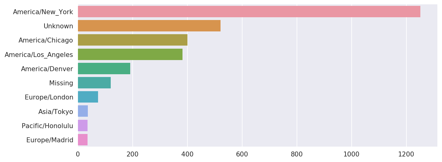
The a field contains
information about the browser, device, or application used to perform
the URL shortening:
In[39]:frame['a'][1]Out[39]:'GoogleMaps/RochesterNY'In[40]:frame['a'][50]Out[40]:'Mozilla/5.0 (Windows NT 5.1; rv:10.0.2) Gecko/20100101 Firefox/10.0.2'In[41]:frame['a'][51][:50]# long lineOut[41]:'Mozilla/5.0 (Linux; U; Android 2.2.2; en-us; LG-P9'
Parsing all of the interesting information in these “agent” strings may seem like a daunting task. One possible strategy is to split off the first token in the string (corresponding roughly to the browser capability) and make another summary of the user behavior:
In[42]:results=pd.Series([x.split()[0]forxinframe.a.dropna()])In[43]:results[:5]Out[43]:0Mozilla/5.01GoogleMaps/RochesterNY2Mozilla/4.03Mozilla/5.04Mozilla/5.0dtype:objectIn[44]:results.value_counts()[:8]Out[44]:Mozilla/5.02594Mozilla/4.0601GoogleMaps/RochesterNY121Opera/9.8034TEST_INTERNET_AGENT24GoogleProducer21Mozilla/6.05BlackBerry8520/5.0.0.6814dtype:int64
Now, suppose you wanted to decompose the top time zones into
Windows and non-Windows users. As a simplification, let’s say that a
user is on Windows if the string 'Windows' is in the agent string. Since some
of the agents are missing, we’ll exclude these from the data:
In[45]:cframe=frame[frame.a.notnull()]
We want to then compute a value for whether each row is Windows or not:
In[47]:cframe['os']=np.where(cframe['a'].str.contains('Windows'),....:'Windows','Not Windows')In[48]:cframe['os'][:5]Out[48]:0Windows1NotWindows2Windows3NotWindows4WindowsName:os,dtype:object
Then, you can group the data by its time zone column and this new list of operating systems:
In[49]:by_tz_os=cframe.groupby(['tz','os'])
The group counts, analogous to the value_counts function, can be computed with
size. This result is then reshaped
into a table with unstack:
In[50]:agg_counts=by_tz_os.size().unstack().fillna(0)In[51]:agg_counts[:10]Out[51]:osNotWindowsWindowstz245.0276.0Africa/Cairo0.03.0Africa/Casablanca0.01.0Africa/Ceuta0.02.0Africa/Johannesburg0.01.0Africa/Lusaka0.01.0America/Anchorage4.01.0America/Argentina/Buenos_Aires1.00.0America/Argentina/Cordoba0.01.0America/Argentina/Mendoza0.01.0
Finally, let’s select the top overall time zones. To do so, I
construct an indirect index array from the row counts in agg_counts:
# Use to sort in ascending orderIn[52]:indexer=agg_counts.sum(1).argsort()In[53]:indexer[:10]Out[53]:tz24Africa/Cairo20Africa/Casablanca21Africa/Ceuta92Africa/Johannesburg87Africa/Lusaka53America/Anchorage54America/Argentina/Buenos_Aires57America/Argentina/Cordoba26America/Argentina/Mendoza55dtype:int64
I use take to select the
rows in that order, then slice off the last 10 rows (largest
values):
In[54]:count_subset=agg_counts.take(indexer[-10:])In[55]:count_subsetOut[55]:osNotWindowsWindowstzAmerica/Sao_Paulo13.020.0Europe/Madrid16.019.0Pacific/Honolulu0.036.0Asia/Tokyo2.035.0Europe/London43.031.0America/Denver132.059.0America/Los_Angeles130.0252.0America/Chicago115.0285.0245.0276.0America/New_York339.0912.0
pandas has a convenience method called nlargest
that does the same thing:
In[56]:agg_counts.sum(1).nlargest(10)Out[56]:tzAmerica/New_York1251.0521.0America/Chicago400.0America/Los_Angeles382.0America/Denver191.0Europe/London74.0Asia/Tokyo37.0Pacific/Honolulu36.0Europe/Madrid35.0America/Sao_Paulo33.0dtype:float64
Then, as shown in the preceding code block, this can be plotted in
a bar plot; I’ll make it a stacked bar plot by passing an additional
argument to seaborn’s barplot function (see Figure 14-2):
# Rearrange the data for plottingIn[58]:count_subset=count_subset.stack()In[59]:count_subset.name='total'In[60]:count_subset=count_subset.reset_index()In[61]:count_subset[:10]Out[61]:tzostotal0America/Sao_PauloNotWindows13.01America/Sao_PauloWindows20.02Europe/MadridNotWindows16.03Europe/MadridWindows19.04Pacific/HonoluluNotWindows0.05Pacific/HonoluluWindows36.06Asia/TokyoNotWindows2.07Asia/TokyoWindows35.08Europe/LondonNotWindows43.09Europe/LondonWindows31.0In[62]:sns.barplot(x='total',y='tz',hue='os',data=count_subset)
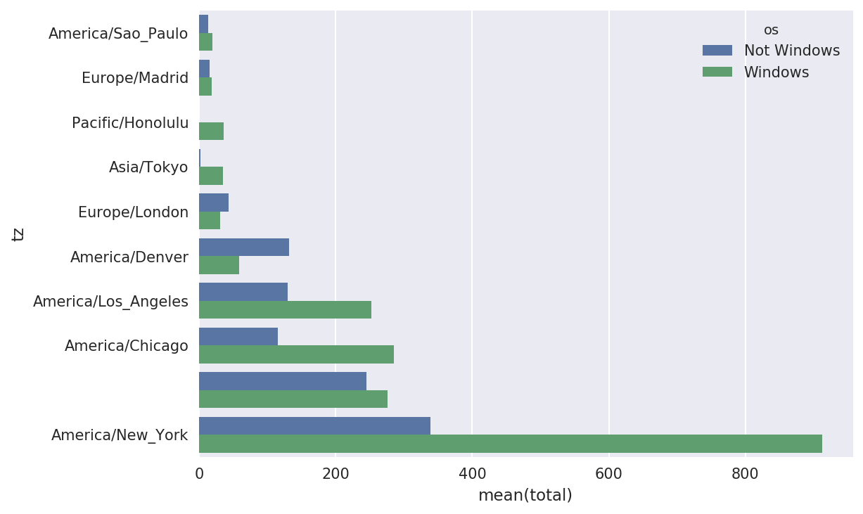
The plot doesn’t make it easy to see the relative percentage of Windows users in the smaller groups, so let’s normalize the group percentages to sum to 1:
defnorm_total(group):group['normed_total']=group.total/group.total.sum()returngroupresults=count_subset.groupby('tz').apply(norm_total)
Then plot this in Figure 14-3:
In[65]:sns.barplot(x='normed_total',y='tz',hue='os',data=results)
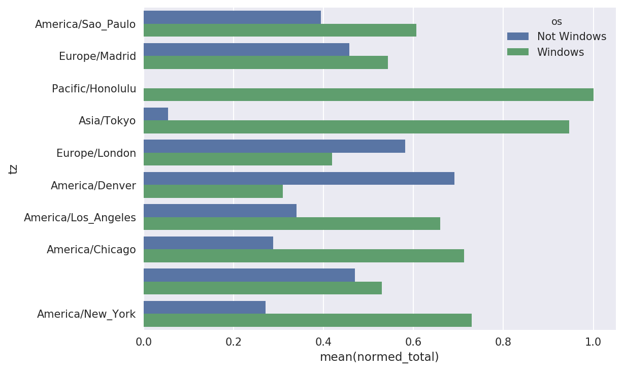
We could have computed the normalized sum more efficiently
by using the transform method with
groupby:
In[66]:g=count_subset.groupby('tz')In[67]:results2=count_subset.total/g.total.transform('sum')
GroupLens Research provides a number of collections of movie ratings data collected from users of MovieLens in the late 1990s and early 2000s. The data provide movie ratings, movie metadata (genres and year), and demographic data about the users (age, zip code, gender identification, and occupation). Such data is often of interest in the development of recommendation systems based on machine learning algorithms. While we do not explore machine learning techniques in detail in this book, I will show you how to slice and dice datasets like these into the exact form you need.
The MovieLens 1M dataset contains 1 million ratings collected from
6,000 users on 4,000 movies. It’s spread across three tables: ratings,
user information, and movie information. After extracting the data from
the ZIP file, we can load each table into a pandas DataFrame object
using pandas.read_table:
importpandasaspd# Make display smallerpd.options.display.max_rows=10unames=['user_id','gender','age','occupation','zip']users=pd.read_table('datasets/movielens/users.dat',sep='::',header=None,names=unames)rnames=['user_id','movie_id','rating','timestamp']ratings=pd.read_table('datasets/movielens/ratings.dat',sep='::',header=None,names=rnames)mnames=['movie_id','title','genres']movies=pd.read_table('datasets/movielens/movies.dat',sep='::',header=None,names=mnames)
You can verify that everything succeeded by looking at the first few rows of each DataFrame with Python’s slice syntax:
In[69]:users[:5]Out[69]:user_idgenderageoccupationzip01F1104806712M56167007223M25155511734M4570246045M252055455In[70]:ratings[:5]Out[70]:user_idmovie_idratingtimestamp011193597830076011661397830210921914397830196831340849783002754123555978824291In[71]:movies[:5]Out[71]:movie_idtitlegenres01ToyStory(1995)Animation|Children's|Comedy12Jumanji(1995)Adventure|Children's|Fantasy23GrumpierOldMen(1995)Comedy|Romance34WaitingtoExhale(1995)Comedy|Drama45FatheroftheBridePartII(1995)ComedyIn[72]:ratingsOut[72]:user_idmovie_idratingtimestamp011193597830076011661397830210921914397830196831340849783002754123555978824291...............1000204604010911956716541100020560401094595670488710002066040562595670474610002076040109649567156481000208604010974956715569[1000209rowsx4columns]
Note that ages and occupations are coded as integers indicating
groups described in the dataset’s README file.
Analyzing the data spread across three tables is not a simple task; for
example, suppose you wanted to compute mean ratings for a particular movie
by sex and age. As you will see, this is much easier to do with all of the
data merged together into a single table. Using pandas’s merge function, we first merge ratings with users and then merge that result with the movies data. pandas infers which columns to use
as the merge (or join) keys based on overlapping
names:
In[73]:data=pd.merge(pd.merge(ratings,users),movies)In[74]:dataOut[74]:user_idmovie_idratingtimestampgenderageoccupationzip\0111935978300760F110480671211935978298413M56167007221211934978220179M25123279331511934978199279M2572290341711935978158471M50195350...........................1000204594921985958846401M1817479011000205567527033976029116M3514300301000206578028451958153068M1817928861000207585136075957756608F1820554101000208593829094957273353M25135401titlegenres0OneFlewOvertheCuckoo's Nest (1975) Drama1OneFlewOvertheCuckoo's Nest (1975) Drama2OneFlewOvertheCuckoo's Nest (1975) Drama3OneFlewOvertheCuckoo's Nest (1975) Drama4OneFlewOvertheCuckoo's Nest (1975) Drama.........1000204Modulations(1998)Documentary1000205BrokenVessels(1998)Drama1000206WhiteBoys(1999)Drama1000207OneLittleIndian(1973)Comedy|Drama|Western1000208FiveWives,ThreeSecretariesandMe(1998)Documentary[1000209rowsx10columns]In[75]:data.iloc[0]Out[75]:user_id1movie_id1193rating5timestamp978300760genderFage1occupation10zip48067titleOneFlewOvertheCuckoo's Nest (1975)genresDramaName:0,dtype:object
To get mean movie ratings for each film grouped by gender, we can
use the pivot_table method:
In[76]:mean_ratings=data.pivot_table('rating',index='title',....:columns='gender',aggfunc='mean')In[77]:mean_ratings[:5]Out[77]:genderFMtitle$1,000,000Duck(1971)3.3750002.761905'Night Mother (1986) 3.388889 3.352941'Til There Was You (1997) 2.675676 2.733333'burbs, The (1989) 2.793478 2.962085...AndJusticeforAll(1979)3.8285713.689024
This produced another DataFrame containing mean ratings with movie
titles as row labels (the “index”) and gender as column labels. I first
filter down to movies that received at least 250 ratings (a completely
arbitrary number); to do this, I then group the data by title and use
size() to get a Series of group sizes
for each title:
In[78]:ratings_by_title=data.groupby('title').size()In[79]:ratings_by_title[:10]Out[79]:title$1,000,000Duck(1971)37'Night Mother (1986) 70'Til There Was You (1997) 52'burbs, The (1989) 303...AndJusticeforAll(1979)1991-900(1994)210ThingsIHateAboutYou(1999)700101Dalmatians(1961)565101Dalmatians(1996)36412AngryMen(1957)616dtype:int64In[80]:active_titles=ratings_by_title.index[ratings_by_title>=250]In[81]:active_titlesOut[81]:Index([''burbs,The(1989)', '10ThingsIHateAboutYou(1999)','101 Dalmatians (1961)','101 Dalmatians (1996)','12 Angry Men (1957)','13th Warrior, The (1999)','2 Days in the Valley (1996)','20,000 Leagues Under the Sea (1954)','2001: A Space Odyssey (1968)','2010 (1984)',...'X-Men (2000)','Year of Living Dangerously (1982)','Yellow Submarine (1968)','You'veGot(1998)','Young Frankenstein (1974)','Young Guns (1988)','Young Guns II (1990)','Young Sherlock Holmes (1985)','Zero Effect (1998)','eXistenZ (1999)'],dtype='object',name='title',length=1216)
The index of titles receiving at least 250 ratings can then be used
to select rows from mean_ratings:
# Select rows on the indexIn[82]:mean_ratings=mean_ratings.loc[active_titles]In[83]:mean_ratingsOut[83]:genderFMtitle'burbs, The (1989) 2.793478 2.96208510ThingsIHateAboutYou(1999)3.6465523.311966101Dalmatians(1961)3.7914443.500000101Dalmatians(1996)3.2400002.91121512AngryMen(1957)4.1843974.328421.........YoungGuns(1988)3.3717953.425620YoungGunsII(1990)2.9347832.904025YoungSherlockHolmes(1985)3.5147063.363344ZeroEffect(1998)3.8644073.723140eXistenZ(1999)3.0985923.289086[1216rowsx2columns]
To see the top films among female viewers, we can sort by the
F column in descending order:
In[85]:top_female_ratings=mean_ratings.sort_values(by='F',ascending=False)In[86]:top_female_ratings[:10]Out[86]:genderFMtitleCloseShave,A(1995)4.6444444.473795WrongTrousers,The(1993)4.5882354.478261SunsetBlvd.(a.k.a.SunsetBoulevard)(1950)4.5726504.464589Wallace&Gromit:TheBestofAardmanAnimation...4.5631074.385075Schindler's List (1993) 4.562602 4.491415ShawshankRedemption,The(1994)4.5390754.560625GrandDayOut,A(1992)4.5378794.293255ToKillaMockingbird(1962)4.5366674.372611CreatureComforts(1990)4.5138894.272277UsualSuspects,The(1995)4.5133174.518248
Suppose you wanted to find the movies that are most divisive
between male and female viewers. One way is to add a column to mean_ratings containing the difference in
means, then sort by that:
In[87]:mean_ratings['diff']=mean_ratings['M']-mean_ratings['F']
Sorting by 'diff' yields the
movies with the greatest rating difference so that we can see which ones
were preferred by women:
In[88]:sorted_by_diff=mean_ratings.sort_values(by='diff')In[89]:sorted_by_diff[:10]Out[89]:genderFMdifftitleDirtyDancing(1987)3.7903782.959596-0.830782Jumpin' Jack Flash (1986) 3.254717 2.578358 -0.676359Grease(1978)3.9752653.367041-0.608224LittleWomen(1994)3.8705883.321739-0.548849SteelMagnolias(1989)3.9017343.365957-0.535777Anastasia(1997)3.8000003.281609-0.518391RockyHorrorPictureShow,The(1975)3.6730163.160131-0.512885ColorPurple,The(1985)4.1581923.659341-0.498851AgeofInnocence,The(1993)3.8270683.339506-0.487561FreeWilly(1993)2.9213482.438776-0.482573
Reversing the order of the rows and again slicing off the top 10 rows, we get the movies preferred by men that women didn’t rate as highly:
# Reverse order of rows, take first 10 rowsIn[90]:sorted_by_diff[::-1][:10]Out[90]:genderFMdifftitleGood,TheBadandTheUgly,The(1966)3.4949494.2213000.726351KentuckyFriedMovie,The(1977)2.8787883.5551470.676359Dumb&Dumber(1994)2.6979873.3365950.638608LongestDay,The(1962)3.4117654.0314470.619682CableGuy,The(1996)2.2500002.8637870.613787EvilDeadII(DeadByDawn)(1987)3.2972973.9092830.611985Hidden,The(1987)3.1379313.7450980.607167RockyIII(1982)2.3617022.9435030.581801Caddyshack(1980)3.3961353.9697370.573602ForaFewDollarsMore(1965)3.4090913.9537950.544704
Suppose instead you wanted the movies that elicited the most disagreement among viewers, independent of gender identification. Disagreement can be measured by the variance or standard deviation of the ratings:
# Standard deviation of rating grouped by titleIn[91]:rating_std_by_title=data.groupby('title')['rating'].std()# Filter down to active_titlesIn[92]:rating_std_by_title=rating_std_by_title.loc[active_titles]# Order Series by value in descending orderIn[93]:rating_std_by_title.sort_values(ascending=False)[:10]Out[93]:titleDumb&Dumber(1994)1.321333BlairWitchProject,The(1999)1.316368NaturalBornKillers(1994)1.307198TankGirl(1995)1.277695RockyHorrorPictureShow,The(1975)1.260177EyesWideShut(1999)1.259624Evita(1996)1.253631BillyMadison(1995)1.249970FearandLoathinginLasVegas(1998)1.246408BicentennialMan(1999)1.245533Name:rating,dtype:float64
You may have noticed that movie genres are given as a
pipe-separated (|) string. If you
wanted to do some analysis by genre, more work would be required to
transform the genre information into a more usable form.
The United States Social Security Administration (SSA) has made available data on the frequency of baby names from 1880 through the present. Hadley Wickham, an author of several popular R packages, has often made use of this dataset in illustrating data manipulation in R.
We need to do some data wrangling to load this dataset, but once we do that we will have a DataFrame that looks like this:
In[4]:names.head(10)Out[4]:namesexbirthsyear0MaryF706518801AnnaF260418802EmmaF200318803ElizabethF193918804MinnieF174618805MargaretF157818806IdaF147218807AliceF141418808BerthaF132018809SarahF12881880
There are many things you might want to do with the dataset:
Visualize the proportion of babies given a particular name (your own, or another name) over time
Determine the relative rank of a name
Determine the most popular names in each year or the names whose popularity has advanced or declined the most
Analyze trends in names: vowels, consonants, length, overall diversity, changes in spelling, first and last letters
Analyze external sources of trends: biblical names, celebrities, demographic changes
With the tools in this book, many of these kinds of analyses are within reach, so I will walk you through some of them.
As of this writing, the US Social Security Administration makes available data files, one per year, containing the total number of births for each sex/name combination. The raw archive of these files can be obtained from http://www.ssa.gov/oact/babynames/limits.html.
In the event that this page has been moved by the time you’re
reading this, it can most likely be located again by an internet search.
After downloading the “National data” file names.zip
and unzipping it, you will have a directory containing a series of files
like yob1880.txt. I use the Unix head command to look at the first 10 lines of
one of the files (on Windows, you can use the more command or open it in a text
editor):
In[94]:!head-n10datasets/babynames/yob1880.txtMary,F,7065Anna,F,2604Emma,F,2003Elizabeth,F,1939Minnie,F,1746Margaret,F,1578Ida,F,1472Alice,F,1414Bertha,F,1320Sarah,F,1288
As this is already in a nicely comma-separated form, it can be
loaded into a DataFrame with pandas.read_csv:
In[95]:importpandasaspdIn[96]:names1880=pd.read_csv('datasets/babynames/yob1880.txt',....:names=['name','sex','births'])In[97]:names1880Out[97]:namesexbirths0MaryF70651AnnaF26042EmmaF20033ElizabethF19394MinnieF1746...........1995WoodieM51996WorthyM51997WrightM51998YorkM51999ZachariahM5[2000rowsx3columns]
These files only contain names with at least five occurrences in each year, so for simplicity’s sake we can use the sum of the births column by sex as the total number of births in that year:
In[98]:names1880.groupby('sex').births.sum()Out[98]:sexF90993M110493Name:births,dtype:int64
Since the dataset is split into files by year, one of the first
things to do is to assemble all of the data into a single DataFrame and
further to add a year field. You can do
this using pandas.concat:
years=range(1880,2011)pieces=[]columns=['name','sex','births']foryearinyears:path='datasets/babynames/yob%d.txt'%yearframe=pd.read_csv(path,names=columns)frame['year']=yearpieces.append(frame)# Concatenate everything into a single DataFramenames=pd.concat(pieces,ignore_index=True)
There are a couple things to note here. First, remember that
concat glues the DataFrame objects
together row-wise by default. Secondly, you have to pass ignore_index=True because we’re not interested
in preserving the original row numbers returned from read_csv. So we now have a very large DataFrame
containing all of the names data:
In[100]:namesOut[100]:namesexbirthsyear0MaryF706518801AnnaF260418802EmmaF200318803ElizabethF193918804MinnieF17461880..............1690779ZymaireM520101690780ZyonneM520101690781ZyquariusM520101690782ZyranM520101690783ZzyzxM52010[1690784rowsx4columns]
With this data in hand, we can already start aggregating the data at
the year and sex level using groupby or
pivot_table (see Figure 14-4):
In[101]:total_births=names.pivot_table('births',index='year',.....:columns='sex',aggfunc=sum)In[102]:total_births.tail()Out[102]:sexFMyear200618964682050234200719168882069242200818836452032310200918276431973359201017590101898382In[103]:total_births.plot(title='Total births by sex and year')
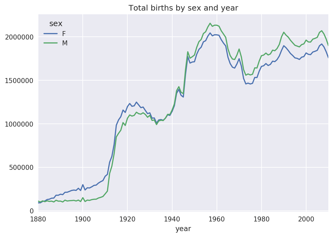
Next, let’s insert a column prop
with the fraction of babies given each name relative to the total number
of births. A prop value of 0.02 would indicate that 2 out of every 100
babies were given a particular name. Thus, we group the data by year and
sex, then add the new column to each group:
defadd_prop(group):group['prop']=group.births/group.births.sum()returngroupnames=names.groupby(['year','sex']).apply(add_prop)
The resulting complete dataset now has the following columns:
In[105]:namesOut[105]:namesexbirthsyearprop0MaryF706518800.0776431AnnaF260418800.0286182EmmaF200318800.0220133ElizabethF193918800.0213094MinnieF174618800.019188.................1690779ZymaireM520100.0000031690780ZyonneM520100.0000031690781ZyquariusM520100.0000031690782ZyranM520100.0000031690783ZzyzxM520100.000003[1690784rowsx5columns]
When performing a group operation like this, it’s often valuable to
do a sanity check, like verifying that the prop column sums to 1 within all the
groups:
In[106]:names.groupby(['year','sex']).prop.sum()Out[106]:yearsex1880F1.0M1.01881F1.0M1.01882F1.0...2008M1.02009F1.0M1.02010F1.0M1.0Name:prop,Length:262,dtype:float64
Now that this is done, I’m going to extract a subset of the data to facilitate further analysis: the top 1,000 names for each sex/year combination. This is yet another group operation:
defget_top1000(group):returngroup.sort_values(by='births',ascending=False)[:1000]grouped=names.groupby(['year','sex'])top1000=grouped.apply(get_top1000)# Drop the group index, not neededtop1000.reset_index(inplace=True,drop=True)
If you prefer a do-it-yourself approach, try this instead:
pieces=[]foryear,groupinnames.groupby(['year','sex']):pieces.append(group.sort_values(by='births',ascending=False)[:1000])top1000=pd.concat(pieces,ignore_index=True)
The resulting dataset is now quite a bit smaller:
In[108]:top1000Out[108]:namesexbirthsyearprop0MaryF706518800.0776431AnnaF260418800.0286182EmmaF200318800.0220133ElizabethF193918800.0213094MinnieF174618800.019188.................261872CamiloM19420100.000102261873DestinM19420100.000102261874JaquanM19420100.000102261875JaydanM19420100.000102261876MaxtonM19320100.000102[261877rowsx5columns]
We’ll use this Top 1,000 dataset in the following investigations into the data.
With the full dataset and Top 1,000 dataset in hand, we can start analyzing various naming trends of interest. Splitting the Top 1,000 names into the boy and girl portions is easy to do first:
In[109]:boys=top1000[top1000.sex=='M']In[110]:girls=top1000[top1000.sex=='F']
Simple time series, like the number of Johns or Marys for each year, can be plotted but require a bit of munging to be more useful. Let’s form a pivot table of the total number of births by year and name:
In[111]:total_births=top1000.pivot_table('births',index='year',.....:columns='name',.....:aggfunc=sum)
Now, this can be plotted for a handful of names with DataFrame’s
plot method (Figure 14-5 shows the result):
In[112]:total_births.info()<class'pandas.core.frame.DataFrame'>Int64Index:131entries,1880to2010Columns:6868entries,AadentoZuridtypes:float64(6868)memoryusage:6.9MBIn[113]:subset=total_births[['John','Harry','Mary','Marilyn']]In[114]:subset.plot(subplots=True,figsize=(12,10),grid=False,.....:title="Number of births per year")
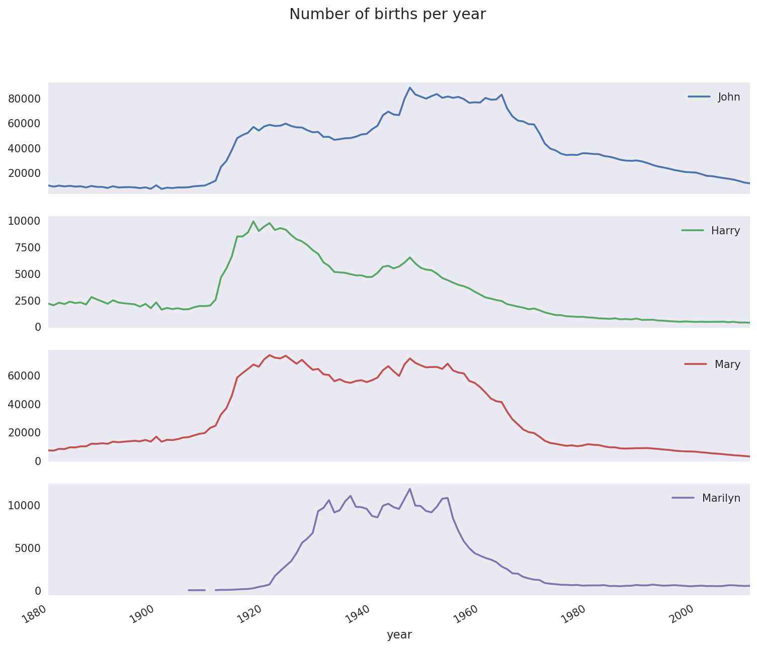
On looking at this, you might conclude that these names have grown out of favor with the American population. But the story is actually more complicated than that, as will be explored in the next section.
One explanation for the decrease in plots is that fewer parents are choosing common names for their children. This hypothesis can be explored and confirmed in the data. One measure is the proportion of births represented by the top 1,000 most popular names, which I aggregate and plot by year and sex (Figure 14-6 shows the resulting plot):
In[116]:table=top1000.pivot_table('prop',index='year',.....:columns='sex',aggfunc=sum)In[117]:table.plot(title='Sum of table1000.prop by year and sex',.....:yticks=np.linspace(0,1.2,13),xticks=range(1880,2020,10))
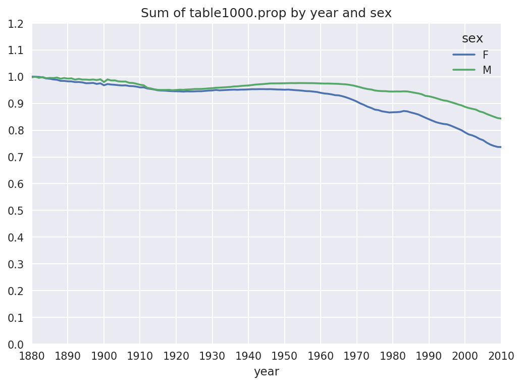
You can see that, indeed, there appears to be increasing name diversity (decreasing total proportion in the top 1,000). Another interesting metric is the number of distinct names, taken in order of popularity from highest to lowest, in the top 50% of births. This number is a bit more tricky to compute. Let’s consider just the boy names from 2010:
In[118]:df=boys[boys.year==2010]In[119]:dfOut[119]:namesexbirthsyearprop260877JacobM2187520100.011523260878EthanM1786620100.009411260879MichaelM1713320100.009025260880JaydenM1703020100.008971260881WilliamM1687020100.008887.................261872CamiloM19420100.000102261873DestinM19420100.000102261874JaquanM19420100.000102261875JaydanM19420100.000102261876MaxtonM19320100.000102[1000rowsx5columns]
After sorting prop in
descending order, we want to know how many of the most popular names
it takes to reach 50%. You could write a for loop to do this, but a vectorized NumPy
way is a bit more clever. Taking the cumulative sum, cumsum, of prop and then calling the method searchsorted returns the position in the
cumulative sum at which 0.5 would
need to be inserted to keep it in sorted order:
In[120]:prop_cumsum=df.sort_values(by='prop',ascending=False).prop.cumsum()In[121]:prop_cumsum[:10]Out[121]:2608770.0115232608780.0209342608790.0299592608800.0389302608810.0478172608820.0565792608830.0651552608840.0734142608850.0815282608860.089621Name:prop,dtype:float64In[122]:prop_cumsum.values.searchsorted(0.5)Out[122]:116
Since arrays are zero-indexed, adding 1 to this result gives you a result of 117. By contrast, in 1900 this number was much smaller:
In[123]:df=boys[boys.year==1900]In[124]:in1900=df.sort_values(by='prop',ascending=False).prop.cumsum()In[125]:in1900.values.searchsorted(0.5)+1Out[125]:25
You can now apply this operation to each year/sex combination,
groupby those fields, and apply a function returning the count for
each group:
defget_quantile_count(group,q=0.5):group=group.sort_values(by='prop',ascending=False)returngroup.prop.cumsum().values.searchsorted(q)+1diversity=top1000.groupby(['year','sex']).apply(get_quantile_count)diversity=diversity.unstack('sex')
This resulting DataFrame diversity now has two time series, one for
each sex, indexed by year. This can be inspected in IPython and
plotted as before (see Figure 14-7):
In[128]:diversity.head()Out[128]:sexFMyear1880381418813814188238151883391518843916In[129]:diversity.plot(title="Number of popular names in top 50%")
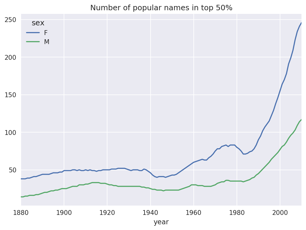
As you can see, girl names have always been more diverse than boy names, and they have only become more so over time. Further analysis of what exactly is driving the diversity, like the increase of alternative spellings, is left to the reader.
In 2007, baby name researcher Laura Wattenberg pointed out on her website that the distribution of boy names by final letter has changed significantly over the last 100 years. To see this, we first aggregate all of the births in the full dataset by year, sex, and final letter:
# extract last letter from name columnget_last_letter=lambdax:x[-1]last_letters=names.name.map(get_last_letter)last_letters.name='last_letter'table=names.pivot_table('births',index=last_letters,columns=['sex','year'],aggfunc=sum)
Then we select out three representative years spanning the history and print the first few rows:
In[131]:subtable=table.reindex(columns=[1910,1960,2010],level='year')In[132]:subtable.head()Out[132]:sexFMyear191019602010191019602010last_lettera108376.0691247.0670605.0977.05204.028438.0bNaN694.0450.0411.03912.038859.0c5.049.0946.0482.015476.023125.0d6750.03729.02607.022111.0262112.044398.0e133569.0435013.0313833.028655.0178823.0129012.0
Next, normalize the table by total births to compute a new table containing proportion of total births for each sex ending in each letter:
In[133]:subtable.sum()Out[133]:sexyearF1910396416.019602022062.020101759010.0M1910194198.019602132588.020101898382.0dtype:float64In[134]:letter_prop=subtable/subtable.sum()In[135]:letter_propOut[135]:sexFMyear191019602010191019602010last_lettera0.2733900.3418530.3812400.0050310.0024400.014980bNaN0.0003430.0002560.0021160.0018340.020470c0.0000130.0000240.0005380.0024820.0072570.012181d0.0170280.0018440.0014820.1138580.1229080.023387e0.3369410.2151330.1784150.1475560.0838530.067959.....................vNaN0.0000600.0001170.0001130.0000370.001434w0.0000200.0000310.0011820.0063290.0077110.016148x0.0000150.0000370.0007270.0039650.0018510.008614y0.1109720.1525690.1168280.0773490.1609870.058168z0.0024390.0006590.0007040.0001700.0001840.001831[26rowsx6columns]
With the letter proportions now in hand, we can make bar plots for each sex broken down by year (see Figure 14-8):
importmatplotlib.pyplotaspltfig,axes=plt.subplots(2,1,figsize=(10,8))letter_prop['M'].plot(kind='bar',rot=0,ax=axes[0],title='Male')letter_prop['F'].plot(kind='bar',rot=0,ax=axes[1],title='Female',legend=False)
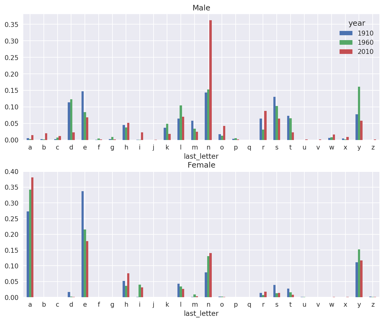
As you can see, boy names ending in n have experienced significant growth since the 1960s. Going back to the full table created before, I again normalize by year and sex and select a subset of letters for the boy names, finally transposing to make each column a time series:
In[138]:letter_prop=table/table.sum()In[139]:dny_ts=letter_prop.loc[['d','n','y'],'M'].TIn[140]:dny_ts.head()Out[140]:last_letterdnyyear18800.0830550.1532130.07576018810.0832470.1532140.07745118820.0853400.1495600.07753718830.0840660.1516460.07914418840.0861200.1499150.080405
With this DataFrame of time series in hand, I can make a plot of
the trends over time again with its plot method (see Figure 14-9):
In[143]:dny_ts.plot()
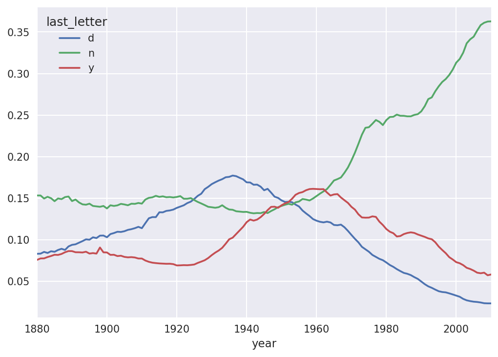
Another fun trend is looking at boy names that were more popular
with one sex earlier in the sample but have “changed sexes” in the
present. One example is the name Lesley or Leslie. Going back to the
top1000 DataFrame, I compute a list
of names occurring in the dataset starting with “lesl”:
In[144]:all_names=pd.Series(top1000.name.unique())In[145]:lesley_like=all_names[all_names.str.lower().str.contains('lesl')]In[146]:lesley_likeOut[146]:632Leslie2294Lesley4262Leslee4728Lesli6103Leslydtype:object
From there, we can filter down to just those names and sum births grouped by name to see the relative frequencies:
In[147]:filtered=top1000[top1000.name.isin(lesley_like)]In[148]:filtered.groupby('name').births.sum()Out[148]:nameLeslee1082Lesley35022Lesli929Leslie370429Lesly10067Name:births,dtype:int64
Next, let’s aggregate by sex and year and normalize within year:
In[149]:table=filtered.pivot_table('births',index='year',.....:columns='sex',aggfunc='sum')In[150]:table=table.div(table.sum(1),axis=0)In[151]:table.tail()Out[151]:sexFMyear20061.0NaN20071.0NaN20081.0NaN20091.0NaN20101.0NaN
Lastly, it’s now possible to make a plot of the breakdown by sex over time (Figure 14-10):
In[153]:table.plot(style={'M':'k-','F':'k--'})
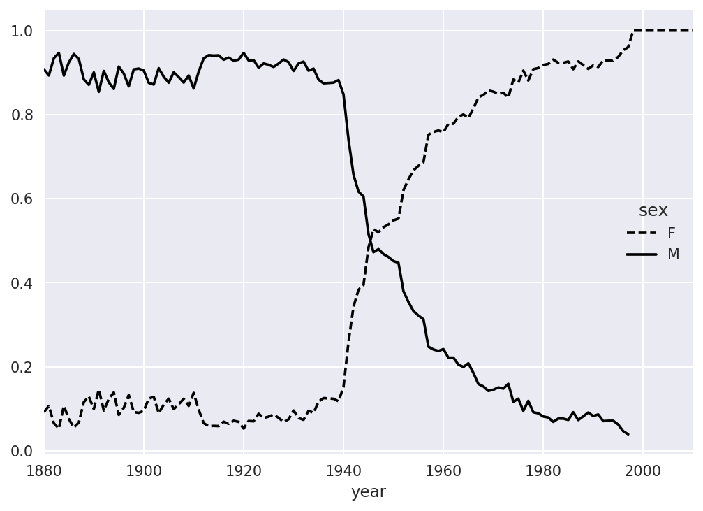
The US Department of Agriculture makes available a database of food nutrient information. Programmer Ashley Williams made available a version of this database in JSON format. The records look like this:
{"id":21441,"description":"KENTUCKY FRIED CHICKEN, Fried Chicken, EXTRA CRISPY,Wing, meat and skin with breading","tags":["KFC"],"manufacturer":"Kentucky Fried Chicken","group":"Fast Foods","portions":[{"amount":1,"unit":"wing, with skin","grams":68.0},...],"nutrients":[{"value":20.8,"units":"g","description":"Protein","group":"Composition"},...]}
Each food has a number of identifying attributes along with two lists of nutrients and portion sizes. Data in this form is not particularly amenable to analysis, so we need to do some work to wrangle the data into a better form.
After downloading and extracting the data from the link, you can
load it into Python with any JSON library of your choosing. I’ll use the
built-in Python json module:
In[154]:importjsonIn[155]:db=json.load(open('datasets/usda_food/database.json'))In[156]:len(db)Out[156]:6636
Each entry in db is a dict
containing all the data for a single food. The 'nutrients' field is a list of dicts, one for
each nutrient:
In[157]:db[0].keys()Out[157]:dict_keys(['id','description','tags','manufacturer','group','portions', 'nutrients'])In[158]:db[0]['nutrients'][0]Out[158]:{'description':'Protein','group':'Composition','units':'g','value':25.18}In[159]:nutrients=pd.DataFrame(db[0]['nutrients'])In[160]:nutrients[:7]Out[160]:descriptiongroupunitsvalue0ProteinCompositiong25.181Totallipid(fat)Compositiong29.202Carbohydrate,bydifferenceCompositiong3.063AshOtherg3.284EnergyEnergykcal376.005WaterCompositiong39.286EnergyEnergykJ1573.00
When converting a list of dicts to a DataFrame, we can specify a list of fields to extract. We’ll take the food names, group, ID, and manufacturer:
In[161]:info_keys=['description','group','id','manufacturer']In[162]:info=pd.DataFrame(db,columns=info_keys)In[163]:info[:5]Out[163]:descriptiongroupid\0Cheese,carawayDairyandEggProducts10081Cheese,cheddarDairyandEggProducts10092Cheese,edamDairyandEggProducts10183Cheese,fetaDairyandEggProducts10194Cheese,mozzarella,partskimmilkDairyandEggProducts1028manufacturer01234In[164]:info.info()<class'pandas.core.frame.DataFrame'>RangeIndex:6636entries,0to6635Datacolumns(total4columns):description6636non-nullobjectgroup6636non-nullobjectid6636non-nullint64manufacturer5195non-nullobjectdtypes:int64(1),object(3)memoryusage:207.5+KB
You can see the distribution of food groups with value_counts:
In[165]:pd.value_counts(info.group)[:10]Out[165]:VegetablesandVegetableProducts812BeefProducts618BakedProducts496BreakfastCereals403LegumesandLegumeProducts365FastFoods365Lamb,Veal,andGameProducts345Sweets341PorkProducts328FruitsandFruitJuices328Name:group,dtype:int64
Now, to do some analysis on all of the nutrient data, it’s easiest
to assemble the nutrients for each food into a single large table. To do
so, we need to take several steps. First, I’ll convert each list of food
nutrients to a DataFrame, add a column for the food id, and append the DataFrame to a list. Then,
these can be concatenated together with concat:
If all goes well, nutrients
should look like this:
In[167]:nutrientsOut[167]:descriptiongroupunitsvalueid0ProteinCompositiong25.18010081Totallipid(fat)Compositiong29.20010082Carbohydrate,bydifferenceCompositiong3.06010083AshOtherg3.28010084EnergyEnergykcal376.0001008..................389350VitaminB-12,addedVitaminsmcg0.00043546389351CholesterolOthermg0.00043546389352Fattyacids,totalsaturatedOtherg0.07243546389353Fattyacids,totalmonounsaturatedOtherg0.02843546389354Fattyacids,totalpolyunsaturatedOtherg0.04143546[389355rowsx5columns]
I noticed that there are duplicates in this DataFrame, so it makes things easier to drop them:
In[168]:nutrients.duplicated().sum()# number of duplicatesOut[168]:14179In[169]:nutrients=nutrients.drop_duplicates()
Since 'group' and 'description' are in both DataFrame objects, we
can rename for clarity:
In[170]:col_mapping={'description':'food',.....:'group':'fgroup'}In[171]:info=info.rename(columns=col_mapping,copy=False)In[172]:info.info()<class'pandas.core.frame.DataFrame'>RangeIndex:6636entries,0to6635Datacolumns(total4columns):food6636non-nullobjectfgroup6636non-nullobjectid6636non-nullint64manufacturer5195non-nullobjectdtypes:int64(1),object(3)memoryusage:207.5+KBIn[173]:col_mapping={'description':'nutrient',.....:'group':'nutgroup'}In[174]:nutrients=nutrients.rename(columns=col_mapping,copy=False)In[175]:nutrientsOut[175]:nutrientnutgroupunitsvalueid0ProteinCompositiong25.18010081Totallipid(fat)Compositiong29.20010082Carbohydrate,bydifferenceCompositiong3.06010083AshOtherg3.28010084EnergyEnergykcal376.0001008..................389350VitaminB-12,addedVitaminsmcg0.00043546389351CholesterolOthermg0.00043546389352Fattyacids,totalsaturatedOtherg0.07243546389353Fattyacids,totalmonounsaturatedOtherg0.02843546389354Fattyacids,totalpolyunsaturatedOtherg0.04143546[375176rowsx5columns]
With all of this done, we’re ready to merge info with nutrients:
In[176]:ndata=pd.merge(nutrients,info,on='id',how='outer')In[177]:ndata.info()<class'pandas.core.frame.DataFrame'>Int64Index:375176entries,0to375175Datacolumns(total8columns):nutrient375176non-nullobjectnutgroup375176non-nullobjectunits375176non-nullobjectvalue375176non-nullfloat64id375176non-nullint64food375176non-nullobjectfgroup375176non-nullobjectmanufacturer293054non-nullobjectdtypes:float64(1),int64(1),object(6)memoryusage:25.8+MBIn[178]:ndata.iloc[30000]Out[178]:nutrientGlycinenutgroupAminoAcidsunitsgvalue0.04id6158foodSoup,tomatobisque,canned,condensedfgroupSoups,Sauces,andGraviesmanufacturerName:30000,dtype:object
We could now make a plot of median values by food group and nutrient type (see Figure 14-11):
In[180]:result=ndata.groupby(['nutrient','fgroup'])['value'].quantile(0.5)In[181]:result['Zinc, Zn'].sort_values().plot(kind='barh')
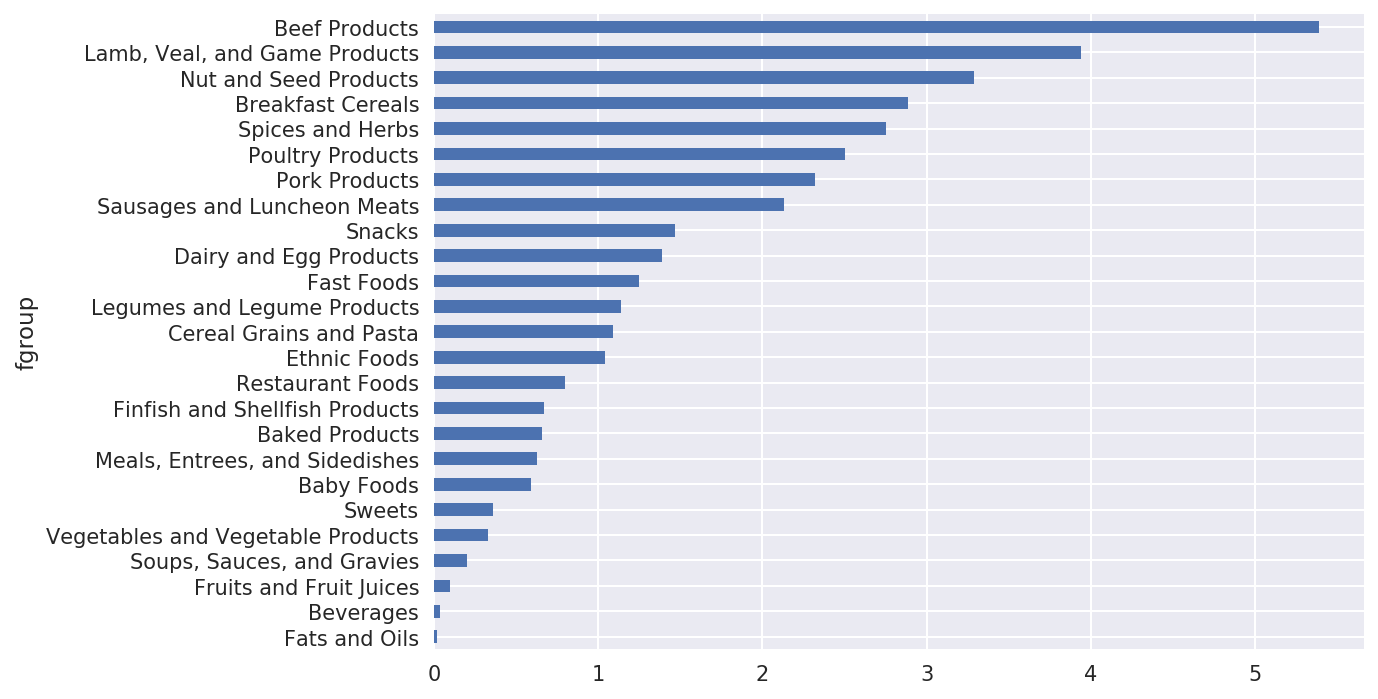
With a little cleverness, you can find which food is most dense in each nutrient:
by_nutrient=ndata.groupby(['nutgroup','nutrient'])get_maximum=lambdax:x.loc[x.value.idxmax()]get_minimum=lambdax:x.loc[x.value.idxmin()]max_foods=by_nutrient.apply(get_maximum)[['value','food']]# make the food a little smallermax_foods.food=max_foods.food.str[:50]
The resulting DataFrame is a bit too large to display in the book;
here is only the 'Amino Acids'
nutrient group:
In[183]:max_foods.loc['Amino Acids']['food']Out[183]:nutrientAlanineGelatins,drypowder,unsweetenedArginineSeeds,sesameflour,low-fatAsparticacidSoyproteinisolateCystineSeeds,cottonseedflour,lowfat(glandless)GlutamicacidSoyproteinisolate...SerineSoyproteinisolate,PROTEINTECHNOLOGIESINTE...ThreonineSoyproteinisolate,PROTEINTECHNOLOGIESINTE...TryptophanSealion,Steller,meatwithfat(AlaskaNative)TyrosineSoyproteinisolate,PROTEINTECHNOLOGIESINTE...ValineSoyproteinisolate,PROTEINTECHNOLOGIESINTE...Name:food,Length:19,dtype:object
The US Federal Election Commission publishes data on contributions to political
campaigns. This includes contributor names, occupation and employer,
address, and contribution amount. An interesting dataset is from the
2012 US presidential election. A version of the dataset I downloaded in
June 2012 is a 150 megabyte CSV file
P00000001-ALL.csv (see the book’s data
repository), which can be loaded with pandas.read_csv:
In[184]:fec=pd.read_csv('datasets/fec/P00000001-ALL.csv')In[185]:fec.info()<class'pandas.core.frame.DataFrame'>RangeIndex:1001731entries,0to1001730Datacolumns(total16columns):cmte_id1001731non-nullobjectcand_id1001731non-nullobjectcand_nm1001731non-nullobjectcontbr_nm1001731non-nullobjectcontbr_city1001712non-nullobjectcontbr_st1001727non-nullobjectcontbr_zip1001620non-nullobjectcontbr_employer988002non-nullobjectcontbr_occupation993301non-nullobjectcontb_receipt_amt1001731non-nullfloat64contb_receipt_dt1001731non-nullobjectreceipt_desc14166non-nullobjectmemo_cd92482non-nullobjectmemo_text97770non-nullobjectform_tp1001731non-nullobjectfile_num1001731non-nullint64dtypes:float64(1),int64(1),object(14)memoryusage:122.3+MB
A sample record in the DataFrame looks like this:
In[186]:fec.iloc[123456]Out[186]:cmte_idC00431445cand_idP80003338cand_nmObama,Barackcontbr_nmELLMAN,IRAcontbr_cityTEMPE...receipt_descNaNmemo_cdNaNmemo_textNaNform_tpSA17Afile_num772372Name:123456,Length:16,dtype:object
You may think of some ways to start slicing and dicing this data to extract informative statistics about donors and patterns in the campaign contributions. I’ll show you a number of different analyses that apply techniques in this book.
You can see that there are no political party affiliations in the
data, so this would be useful to add. You can get a list of all the unique
political candidates using unique:
In[187]:unique_cands=fec.cand_nm.unique()In[188]:unique_candsOut[188]:array(['Bachmann, Michelle','Romney, Mitt','Obama, Barack',"Roemer, Charles E. 'Buddy' III",'Pawlenty, Timothy','Johnson, Gary Earl','Paul, Ron','Santorum, Rick','Cain, Herman','Gingrich, Newt','McCotter, Thaddeus G','Huntsman, Jon','Perry, Rick'],dtype=object)In[189]:unique_cands[2]Out[189]:'Obama, Barack'
One way to indicate party affiliation is using a dict:1
parties={'Bachmann, Michelle':'Republican','Cain, Herman':'Republican','Gingrich, Newt':'Republican','Huntsman, Jon':'Republican','Johnson, Gary Earl':'Republican','McCotter, Thaddeus G':'Republican','Obama, Barack':'Democrat','Paul, Ron':'Republican','Pawlenty, Timothy':'Republican','Perry, Rick':'Republican',"Roemer, Charles E. 'Buddy' III":'Republican','Romney, Mitt':'Republican','Santorum, Rick':'Republican'}
Now, using this mapping and the map method on Series objects, you can compute an
array of political parties from the candidate names:
In[191]:fec.cand_nm[123456:123461]Out[191]:123456Obama,Barack123457Obama,Barack123458Obama,Barack123459Obama,Barack123460Obama,BarackName:cand_nm,dtype:objectIn[192]:fec.cand_nm[123456:123461].map(parties)Out[192]:123456Democrat123457Democrat123458Democrat123459Democrat123460DemocratName:cand_nm,dtype:object# Add it as a columnIn[193]:fec['party']=fec.cand_nm.map(parties)In[194]:fec['party'].value_counts()Out[194]:Democrat593746Republican407985Name:party,dtype:int64
A couple of data preparation points. First, this data includes both contributions and refunds (negative contribution amount):
In[195]:(fec.contb_receipt_amt>0).value_counts()Out[195]:True991475False10256Name:contb_receipt_amt,dtype:int64
To simplify the analysis, I’ll restrict the dataset to positive contributions:
In[196]:fec=fec[fec.contb_receipt_amt>0]
Since Barack Obama and Mitt Romney were the main two candidates, I’ll also prepare a subset that just has contributions to their campaigns:
In[197]:fec_mrbo=fec[fec.cand_nm.isin(['Obama, Barack','Romney, Mitt'])]
Donations by occupation is another oft-studied statistic. For example, lawyers (attorneys) tend to donate more money to Democrats, while business executives tend to donate more to Republicans. You have no reason to believe me; you can see for yourself in the data. First, the total number of donations by occupation is easy:
In[198]:fec.contbr_occupation.value_counts()[:10]Out[198]:RETIRED233990INFORMATIONREQUESTED35107ATTORNEY34286HOMEMAKER29931PHYSICIAN23432INFORMATIONREQUESTEDPERBESTEFFORTS21138ENGINEER14334TEACHER13990CONSULTANT13273PROFESSOR12555Name:contbr_occupation,dtype:int64
You will notice by looking at the occupations that many refer to
the same basic job type, or there are several variants of the same
thing. The following code snippet illustrates a technique for cleaning
up a few of them by mapping from one occupation to another; note the
“trick” of using dict.get to allow
occupations with no mapping to “pass through”:
occ_mapping={'INFORMATION REQUESTED PER BEST EFFORTS':'NOT PROVIDED','INFORMATION REQUESTED':'NOT PROVIDED','INFORMATION REQUESTED (BEST EFFORTS)':'NOT PROVIDED','C.E.O.':'CEO'}# If no mapping provided, return xf=lambdax:occ_mapping.get(x,x)fec.contbr_occupation=fec.contbr_occupation.map(f)
I’ll also do the same thing for employers:
emp_mapping={'INFORMATION REQUESTED PER BEST EFFORTS':'NOT PROVIDED','INFORMATION REQUESTED':'NOT PROVIDED','SELF':'SELF-EMPLOYED','SELF EMPLOYED':'SELF-EMPLOYED',}# If no mapping provided, return xf=lambdax:emp_mapping.get(x,x)fec.contbr_employer=fec.contbr_employer.map(f)
Now, you can use pivot_table to
aggregate the data by party and occupation, then filter down to the
subset that donated at least $2 million overall:
In[201]:by_occupation=fec.pivot_table('contb_receipt_amt',.....:index='contbr_occupation',.....:columns='party',aggfunc='sum')In[202]:over_2mm=by_occupation[by_occupation.sum(1)>2000000]In[203]:over_2mmOut[203]:partyDemocratRepublicancontbr_occupationATTORNEY11141982.977.477194e+06CEO2074974.794.211041e+06CONSULTANT2459912.712.544725e+06ENGINEER951525.551.818374e+06EXECUTIVE1355161.054.138850e+06.........PRESIDENT1878509.954.720924e+06PROFESSOR2165071.082.967027e+05REALESTATE528902.091.625902e+06RETIRED25305116.382.356124e+07SELF-EMPLOYED672393.401.640253e+06[17rowsx2columns]
It can be easier to look at this data graphically as a bar plot
('barh' means horizontal bar plot;
see Figure 14-12):
In[205]:over_2mm.plot(kind='barh')
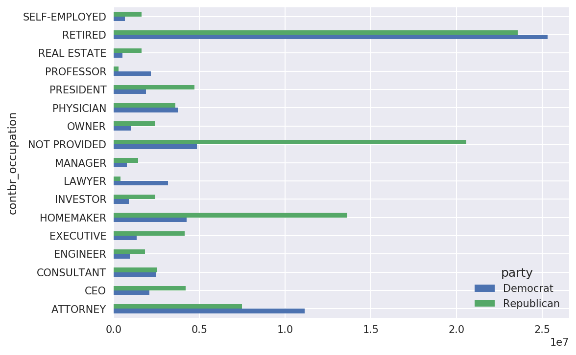
You might be interested in the top donor occupations or top
companies that donated to Obama and Romney. To do this, you can group by
candidate name and use a variant of the top method from earlier in the chapter:
defget_top_amounts(group,key,n=5):totals=group.groupby(key)['contb_receipt_amt'].sum()returntotals.nlargest(n)
Then aggregate by occupation and employer:
In[207]:grouped=fec_mrbo.groupby('cand_nm')In[208]:grouped.apply(get_top_amounts,'contbr_occupation',n=7)Out[208]:cand_nmcontbr_occupationObama,BarackRETIRED25305116.38ATTORNEY11141982.97INFORMATIONREQUESTED4866973.96HOMEMAKER4248875.80PHYSICIAN3735124.94...Romney,MittHOMEMAKER8147446.22ATTORNEY5364718.82PRESIDENT2491244.89EXECUTIVE2300947.03C.E.O.1968386.11Name:contb_receipt_amt,Length:14,dtype:float64In[209]:grouped.apply(get_top_amounts,'contbr_employer',n=10)Out[209]:cand_nmcontbr_employerObama,BarackRETIRED22694358.85SELF-EMPLOYED17080985.96NOTEMPLOYED8586308.70INFORMATIONREQUESTED5053480.37HOMEMAKER2605408.54...Romney,MittCREDITSUISSE281150.00MORGANSTANLEY267266.00GOLDMANSACH&CO.238250.00BARCLAYSCAPITAL162750.00H.I.G.CAPITAL139500.00Name:contb_receipt_amt,Length:20,dtype:float64
A useful way to analyze this data is to use the cut function to discretize the contributor
amounts into buckets by contribution size:
In[210]:bins=np.array([0,1,10,100,1000,10000,.....:100000,1000000,10000000])In[211]:labels=pd.cut(fec_mrbo.contb_receipt_amt,bins)In[212]:labelsOut[212]:411(10,100]412(100,1000]413(100,1000]414(10,100]415(10,100]...701381(10,100]701382(100,1000]701383(1,10]701384(10,100]701385(100,1000]Name:contb_receipt_amt,Length:694282,dtype:categoryCategories(8,interval[int64]):[(0,1]<(1,10]<(10,100]<(100,1000]<(1000,10000]<(10000,100000]<(100000,1000000]<(1000000,10000000]]
We can then group the data for Obama and Romney by name and bin label to get a histogram by donation size:
In[213]:grouped=fec_mrbo.groupby(['cand_nm',labels])In[214]:grouped.size().unstack(0)Out[214]:cand_nmObama,BarackRomney,Mittcontb_receipt_amt(0,1]493.077.0(1,10]40070.03681.0(10,100]372280.031853.0(100,1000]153991.043357.0(1000,10000]22284.026186.0(10000,100000]2.01.0(100000,1000000]3.0NaN(1000000,10000000]4.0NaN
This data shows that Obama received a significantly larger number of small donations than Romney. You can also sum the contribution amounts and normalize within buckets to visualize percentage of total donations of each size by candidate (Figure 14-13 shows the resulting plot):
In[216]:bucket_sums=grouped.contb_receipt_amt.sum().unstack(0)In[217]:normed_sums=bucket_sums.div(bucket_sums.sum(axis=1),axis=0)In[218]:normed_sumsOut[218]:cand_nmObama,BarackRomney,Mittcontb_receipt_amt(0,1]0.8051820.194818(1,10]0.9187670.081233(10,100]0.9107690.089231(100,1000]0.7101760.289824(1000,10000]0.4473260.552674(10000,100000]0.8231200.176880(100000,1000000]1.000000NaN(1000000,10000000]1.000000NaNIn[219]:normed_sums[:-2].plot(kind='barh')
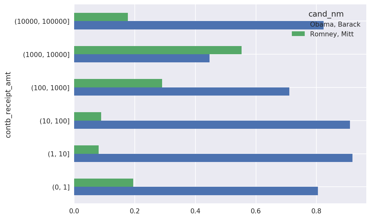
I excluded the two largest bins as these are not donations by individuals.
This analysis can be refined and improved in many ways. For example, you could aggregate donations by donor name and zip code to adjust for donors who gave many small amounts versus one or more large donations. I encourage you to download and explore the dataset yourself.
Aggregating the data by candidate and state is a routine affair:
In[220]:grouped=fec_mrbo.groupby(['cand_nm','contbr_st'])In[221]:totals=grouped.contb_receipt_amt.sum().unstack(0).fillna(0)In[222]:totals=totals[totals.sum(1)>100000]In[223]:totals[:10]Out[223]:cand_nmObama,BarackRomney,Mittcontbr_stAK281840.1586204.24AL543123.48527303.51AR359247.28105556.00AZ1506476.981888436.23CA23824984.2411237636.60CO2132429.491506714.12CT2068291.263499475.45DC4373538.801025137.50DE336669.1482712.00FL7318178.588338458.81
If you divide each row by the total contribution amount, you get the relative percentage of total donations by state for each candidate:
In[224]:percent=totals.div(totals.sum(1),axis=0)In[225]:percent[:10]Out[225]:cand_nmObama,BarackRomney,Mittcontbr_stAK0.7657780.234222AL0.5073900.492610AR0.7729020.227098AZ0.4437450.556255CA0.6794980.320502CO0.5859700.414030CT0.3714760.628524DC0.8101130.189887DE0.8027760.197224FL0.4674170.532583
We’ve reached the end of the book’s main chapters. I have included some additional content you may find useful in the appendixes.
In the five years since the first edition of this book was published, Python has become a popular and widespread language for data analysis. The programming skills you have developed here will stay relevant for a long time into the future. I hope the programming tools and libraries we’ve explored serve you well in your work.
1 This makes the simplifying assumption that Gary Johnson is a Republican even though he later became the Libertarian party candidate.
In this appendix, I will go deeper into the NumPy library for array computing. This will include more internal detail about the ndarray type and more advanced array manipulations and algorithms.
This appendix contains miscellaneous topics and does not necessarily need to be read linearly.
The NumPy ndarray provides a means to interpret a block of homogeneous data (either contiguous or strided) as a multidimensional array object. The data type, or dtype, determines how the data is interpreted as being floating point, integer, boolean, or any of the other types we’ve been looking at.
Part of what makes ndarray flexible is that every array object is a
strided view on a block of data. You might wonder,
for example, how the array view arr[::2,
::-1] does not copy any data. The reason is that the ndarray is
more than just a chunk of memory and a dtype; it also has “striding”
information that enables the array to move through memory with varying
step sizes. More precisely, the ndarray internally consists of the
following:
A pointer to data—that is, a block of data in RAM or in a memory-mapped file
The data type or dtype, describing fixed-size value cells in the array
A tuple indicating the array’s shape
A tuple of strides, integers indicating the number of bytes to “step” in order to advance one element along a dimension
See Figure A-1 for a simple mockup of the ndarray innards.
For example, a 10 × 5 array would have shape (10, 5):
In[10]:np.ones((10,5)).shapeOut[10]:(10,5)
A typical (C order) 3 × 4 × 5 array of float64 (8-byte) values has strides (160, 40, 8) (knowing about the strides can be
useful because, in general, the larger the strides on a particular axis,
the more costly it is to perform computation along that axis):
In[11]:np.ones((3,4,5),dtype=np.float64).stridesOut[11]:(160,40,8)
While it is rare that a typical NumPy user would be interested in
the array strides, they are the critical ingredient in
constructing “zero-copy” array views. Strides can even be negative,
which enables an array to move “backward” through memory (this would be
the case, for example, in a slice like obj[::-1] or obj[:,
::-1]).
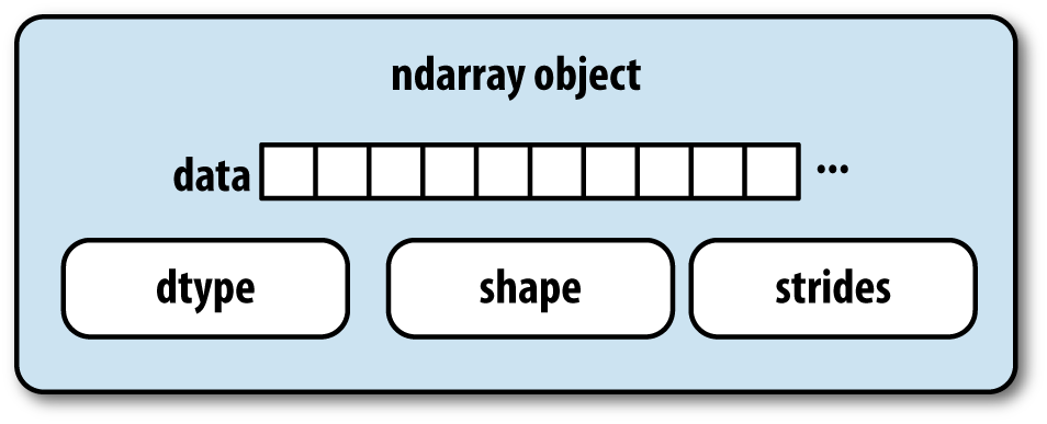
You may occasionally have code that needs to check whether an array contains
integers, floating-point numbers, strings, or Python objects. Because
there are multiple types of floating-point numbers (float16 through float128), checking that the dtype is among a
list of types would be very verbose. Fortunately, the dtypes have
superclasses such as np.integer and
np.floating, which can be used in
conjunction with the np.issubdtype
function:
In[12]:ints=np.ones(10,dtype=np.uint16)In[13]:floats=np.ones(10,dtype=np.float32)In[14]:np.issubdtype(ints.dtype,np.integer)Out[14]:TrueIn[15]:np.issubdtype(floats.dtype,np.floating)Out[15]:True
You can see all of the parent classes of a specific dtype by
calling the type’s mro
method:
In[16]:np.float64.mro()Out[16]:[numpy.float64,numpy.floating,numpy.inexact,numpy.number,numpy.generic,float,object]
Therefore, we also have:
In[17]:np.issubdtype(ints.dtype,np.number)Out[17]:True
Most NumPy users will never have to know about this, but it occasionally comes in handy. See Figure A-2 for a graph of the dtype hierarchy and parent–subclass relationships.1
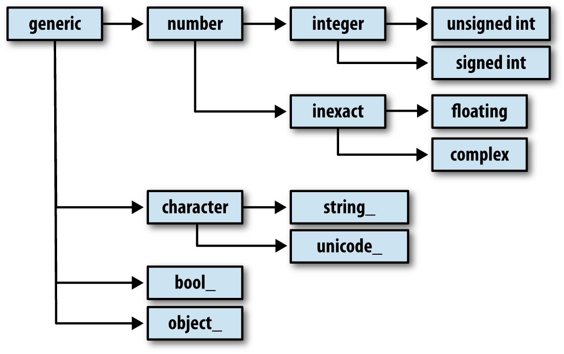
There are many ways to work with arrays beyond fancy indexing, slicing, and boolean subsetting. While much of the heavy lifting for data analysis applications is handled by higher-level functions in pandas, you may at some point need to write a data algorithm that is not found in one of the existing libraries.
In many cases, you can convert an array from one shape to another without
copying any data. To do this, pass a tuple indicating the new shape to
the reshape array instance method.
For example, suppose we had a one-dimensional array of values that we
wished to rearrange into a matrix (the result is shown in Figure A-3):
In[18]:arr=np.arange(8)In[19]:arrOut[19]:array([0,1,2,3,4,5,6,7])In[20]:arr.reshape((4,2))Out[20]:array([[0,1],[2,3],[4,5],[6,7]])
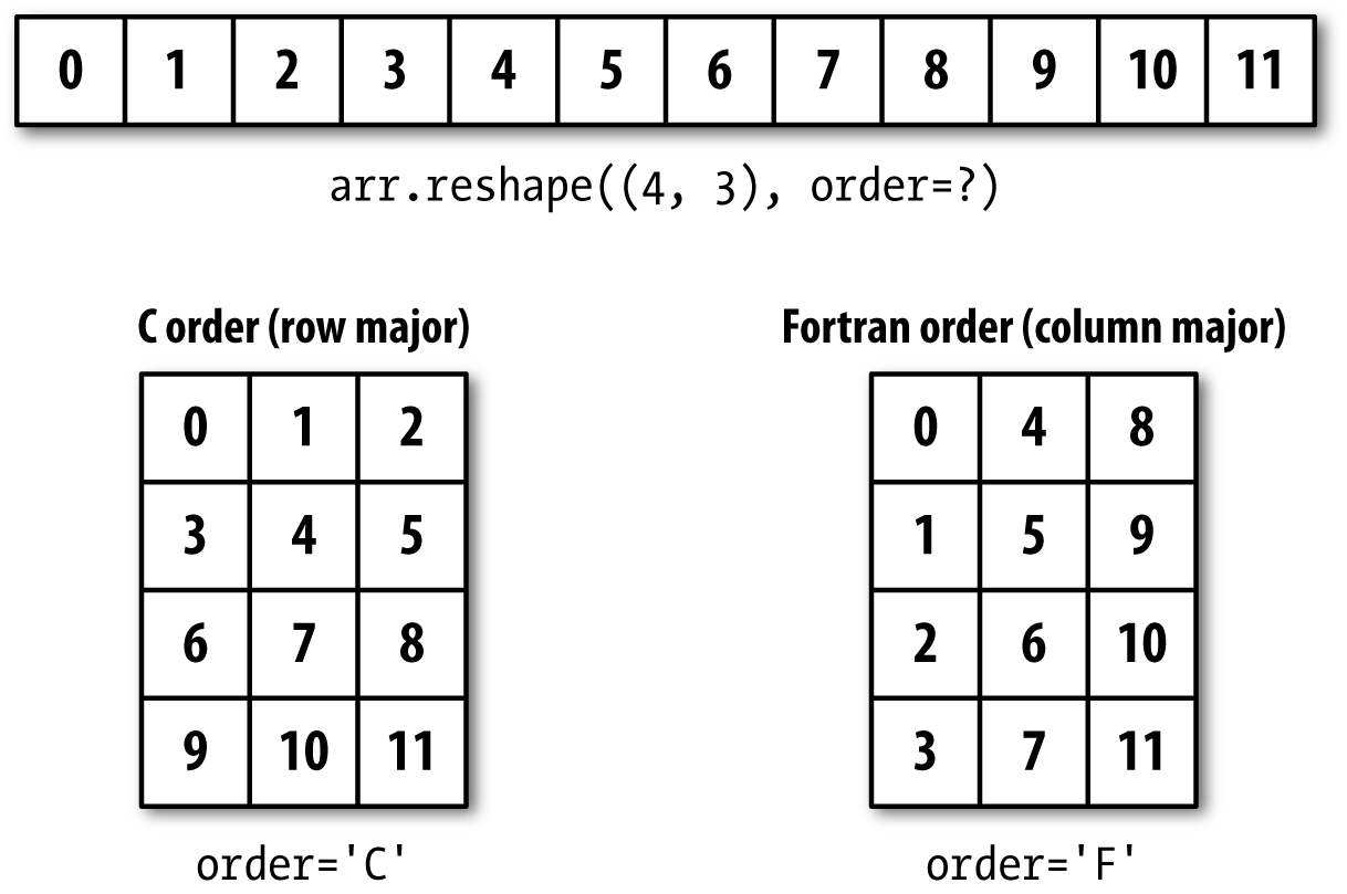
A multidimensional array can also be reshaped:
In[21]:arr.reshape((4,2)).reshape((2,4))Out[21]:array([[0,1,2,3],[4,5,6,7]])
One of the passed shape dimensions can be –1, in which case the value used for that dimension will be inferred from the data:
In[22]:arr=np.arange(15)In[23]:arr.reshape((5,-1))Out[23]:array([[0,1,2],[3,4,5],[6,7,8],[9,10,11],[12,13,14]])
Since an array’s shape
attribute is a tuple, it can be passed to reshape, too:
In[24]:other_arr=np.ones((3,5))In[25]:other_arr.shapeOut[25]:(3,5)In[26]:arr.reshape(other_arr.shape)Out[26]:array([[0,1,2,3,4],[5,6,7,8,9],[10,11,12,13,14]])
The opposite operation of reshape from one-dimensional to a higher
dimension is typically known as flattening or
raveling:
In[27]:arr=np.arange(15).reshape((5,3))In[28]:arrOut[28]:array([[0,1,2],[3,4,5],[6,7,8],[9,10,11],[12,13,14]])In[29]:arr.ravel()Out[29]:array([0,1,2,3,4,5,6,7,8,9,10,11,12,13,14])
ravel does not produce a copy
of the underlying values if the values in the result were contiguous in the original array.
The flatten method behaves like ravel
except it always returns a copy of the data:
In[30]:arr.flatten()Out[30]:array([0,1,2,3,4,5,6,7,8,9,10,11,12,13,14])
The data can be reshaped or raveled in different orders. This is a slightly nuanced topic for new NumPy users and is therefore the next subtopic.
NumPy gives you control and flexibility over the layout of your data in memory. By default, NumPy arrays are created in row major order. Spatially this means that if you have a two-dimensional array of data, the items in each row of the array are stored in adjacent memory locations. The alternative to row major ordering is column major order, which means that values within each column of data are stored in adjacent memory locations.
For historical reasons, row and column major order are also know as C and Fortran order, respectively. In the FORTRAN 77 language, matrices are all column major.
Functions like reshape and
ravel accept an order argument indicating the order to use the
data in the array. This is usually set to 'C' or 'F'
in most cases (there are also less commonly used options 'A' and 'K'; see the NumPy documentation, and refer
back to Figure A-3 for an illustration of
these options):
In[31]:arr=np.arange(12).reshape((3,4))In[32]:arrOut[32]:array([[0,1,2,3],[4,5,6,7],[8,9,10,11]])In[33]:arr.ravel()Out[33]:array([0,1,2,3,4,5,6,7,8,9,10,11])In[34]:arr.ravel('F')Out[34]:array([0,4,8,1,5,9,2,6,10,3,7,11])
Reshaping arrays with more than two dimensions can be a bit mind-bending (see Figure A-3). The key difference between C and Fortran order is the way in which the dimensions are walked:
Traverse higher dimensions first (e.g., axis 1 before advancing on axis 0).
Traverse higher dimensions last (e.g., axis 0 before advancing on axis 1).
numpy.concatenate takes a
sequence (tuple, list, etc.) of arrays and joins them
together in order along the input axis:
In[35]:arr1=np.array([[1,2,3],[4,5,6]])In[36]:arr2=np.array([[7,8,9],[10,11,12]])In[37]:np.concatenate([arr1,arr2],axis=0)Out[37]:array([[1,2,3],[4,5,6],[7,8,9],[10,11,12]])In[38]:np.concatenate([arr1,arr2],axis=1)Out[38]:array([[1,2,3,7,8,9],[4,5,6,10,11,12]])
There are some convenience functions, like vstack and
hstack, for common kinds of
concatenation. The preceding operations could have been expressed
as:
In[39]:np.vstack((arr1,arr2))Out[39]:array([[1,2,3],[4,5,6],[7,8,9],[10,11,12]])In[40]:np.hstack((arr1,arr2))Out[40]:array([[1,2,3,7,8,9],[4,5,6,10,11,12]])
split, on the other hand, slices apart an array into multiple arrays along an
axis:
In[41]:arr=np.random.randn(5,2)In[42]:arrOut[42]:array([[-0.2047,0.4789],[-0.5194,-0.5557],[1.9658,1.3934],[0.0929,0.2817],[0.769,1.2464]])In[43]:first,second,third=np.split(arr,[1,3])In[44]:firstOut[44]:array([[-0.2047,0.4789]])In[45]:secondOut[45]:array([[-0.5194,-0.5557],[1.9658,1.3934]])In[46]:thirdOut[46]:array([[0.0929,0.2817],[0.769,1.2464]])
The value [1, 3] passed to
np.split indicate the indices at which to split the
array into pieces.
See Table A-1 for a list of all
relevant concatenation and splitting functions, some of which are
provided only as a convenience of the very general-purpose concatenate.
There are two special objects in the NumPy namespace, r_
and c_, that make stacking arrays
more concise:
In[47]:arr=np.arange(6)In[48]:arr1=arr.reshape((3,2))In[49]:arr2=np.random.randn(3,2)In[50]:np.r_[arr1,arr2]Out[50]:array([[0.,1.],[2.,3.],[4.,5.],[1.0072,-1.2962],[0.275,0.2289],[1.3529,0.8864]])In[51]:np.c_[np.r_[arr1,arr2],arr]Out[51]:array([[0.,1.,0.],[2.,3.,1.],[4.,5.,2.],[1.0072,-1.2962,3.],[0.275,0.2289,4.],[1.3529,0.8864,5.]])
These additionally can translate slices to arrays:
In[52]:np.c_[1:6,-10:-5]Out[52]:array([[1,-10],[2,-9],[3,-8],[4,-7],[5,-6]])
See the docstring for more on what you can do with c_ and r_.
Two useful tools for repeating or replicating arrays to produce
larger arrays are the repeat and tile functions. repeat replicates each element in an array
some number of times, producing a larger array:
In[53]:arr=np.arange(3)In[54]:arrOut[54]:array([0,1,2])In[55]:arr.repeat(3)Out[55]:array([0,0,0,1,1,1,2,2,2])
The need to replicate or repeat arrays can be less common with NumPy than it is with other array programming frameworks like MATLAB. One reason for this is that broadcasting often fills this need better, which is the subject of the next section.
By default, if you pass an integer, each element will be repeated that number of times. If you pass an array of integers, each element can be repeated a different number of times:
In[56]:arr.repeat([2,3,4])Out[56]:array([0,0,1,1,1,2,2,2,2])
Multidimensional arrays can have their elements repeated along a particular axis.
In[57]:arr=np.random.randn(2,2)In[58]:arrOut[58]:array([[-2.0016,-0.3718],[1.669,-0.4386]])In[59]:arr.repeat(2,axis=0)Out[59]:array([[-2.0016,-0.3718],[-2.0016,-0.3718],[1.669,-0.4386],[1.669,-0.4386]])
Note that if no axis is passed, the array will be flattened first, which is likely not what you want. Similarly, you can pass an array of integers when repeating a multidimensional array to repeat a given slice a different number of times:
In[60]:arr.repeat([2,3],axis=0)Out[60]:array([[-2.0016,-0.3718],[-2.0016,-0.3718],[1.669,-0.4386],[1.669,-0.4386],[1.669,-0.4386]])In[61]:arr.repeat([2,3],axis=1)Out[61]:array([[-2.0016,-2.0016,-0.3718,-0.3718,-0.3718],[1.669,1.669,-0.4386,-0.4386,-0.4386]])
tile, on the other hand, is a
shortcut for stacking copies of an array along an axis. Visually you can
think of it as being akin to “laying down tiles”:
In[62]:arrOut[62]:array([[-2.0016,-0.3718],[1.669,-0.4386]])In[63]:np.tile(arr,2)Out[63]:array([[-2.0016,-0.3718,-2.0016,-0.3718],[1.669,-0.4386,1.669,-0.4386]])
The second argument is the number of tiles; with a scalar, the
tiling is made row by row, rather than column by column. The second
argument to tile can be a tuple
indicating the layout of the “tiling”:
In[64]:arrOut[64]:array([[-2.0016,-0.3718],[1.669,-0.4386]])In[65]:np.tile(arr,(2,1))Out[65]:array([[-2.0016,-0.3718],[1.669,-0.4386],[-2.0016,-0.3718],[1.669,-0.4386]])In[66]:np.tile(arr,(3,2))Out[66]:array([[-2.0016,-0.3718,-2.0016,-0.3718],[1.669,-0.4386,1.669,-0.4386],[-2.0016,-0.3718,-2.0016,-0.3718],[1.669,-0.4386,1.669,-0.4386],[-2.0016,-0.3718,-2.0016,-0.3718],[1.669,-0.4386,1.669,-0.4386]])
As you may recall from Chapter 4, one way to get and set subsets of arrays is by fancy indexing using integer arrays:
In[67]:arr=np.arange(10)*100In[68]:inds=[7,1,2,6]In[69]:arr[inds]Out[69]:array([700,100,200,600])
There are alternative ndarray methods that are useful in the special case of only making a selection on a single axis:
In[70]:arr.take(inds)Out[70]:array([700,100,200,600])In[71]:arr.put(inds,42)In[72]:arrOut[72]:array([0,42,42,300,400,500,42,42,800,900])In[73]:arr.put(inds,[40,41,42,43])In[74]:arrOut[74]:array([0,41,42,300,400,500,43,40,800,900])
To use take along other axes,
you can pass the axis keyword:
In[75]:inds=[2,0,2,1]In[76]:arr=np.random.randn(2,4)In[77]:arrOut[77]:array([[-0.5397,0.477,3.2489,-1.0212],[-0.5771,0.1241,0.3026,0.5238]])In[78]:arr.take(inds,axis=1)Out[78]:array([[3.2489,-0.5397,3.2489,0.477],[0.3026,-0.5771,0.3026,0.1241]])
put does not accept an axis argument but rather indexes into the
flattened (one-dimensional, C order) version of the array. Thus, when
you need to set elements using an index array on other axes, it is often
easiest to use fancy indexing.
Broadcasting describes how arithmetic works between arrays of different shapes. It can be a powerful feature, but one that can cause confusion, even for experienced users. The simplest example of broadcasting occurs when combining a scalar value with an array:
In[79]:arr=np.arange(5)In[80]:arrOut[80]:array([0,1,2,3,4])In[81]:arr*4Out[81]:array([0,4,8,12,16])
Here we say that the scalar value 4 has been broadcast to all of the other elements in the multiplication operation.
For example, we can demean each column of an array by subtracting the column means. In this case, it is very simple:
In[82]:arr=np.random.randn(4,3)In[83]:arr.mean(0)Out[83]:array([-0.3928,-0.3824,-0.8768])In[84]:demeaned=arr-arr.mean(0)In[85]:demeanedOut[85]:array([[0.3937,1.7263,0.1633],[-0.4384,-1.9878,-0.9839],[-0.468,0.9426,-0.3891],[0.5126,-0.6811,1.2097]])In[86]:demeaned.mean(0)Out[86]:array([-0.,0.,-0.])
See Figure A-4 for an illustration of this operation. Demeaning the rows as a broadcast operation requires a bit more care. Fortunately, broadcasting potentially lower dimensional values across any dimension of an array (like subtracting the row means from each column of a two-dimensional array) is possible as long as you follow the rules.
This brings us to:
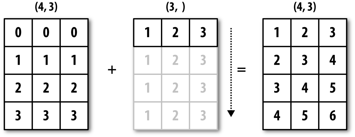
Even as an experienced NumPy user, I often find myself having to
pause and draw a diagram as I think about the broadcasting rule. Consider
the last example and suppose we wished instead to subtract the mean value
from each row. Since arr.mean(0) has
length 3, it is compatible for broadcasting across axis 0 because the
trailing dimension in arr is 3 and
therefore matches. According to the rules, to subtract over axis 1 (i.e.,
subtract the row mean from each row), the smaller array must have shape
(4, 1):
In[87]:arrOut[87]:array([[0.0009,1.3438,-0.7135],[-0.8312,-2.3702,-1.8608],[-0.8608,0.5601,-1.2659],[0.1198,-1.0635,0.3329]])In[88]:row_means=arr.mean(1)In[89]:row_means.shapeOut[89]:(4,)In[90]:row_means.reshape((4,1))Out[90]:array([[0.2104],[-1.6874],[-0.5222],[-0.2036]])In[91]:demeaned=arr-row_means.reshape((4,1))In[92]:demeaned.mean(1)Out[92]:array([0.,-0.,0.,0.])
See Figure A-5 for an illustration of this operation.
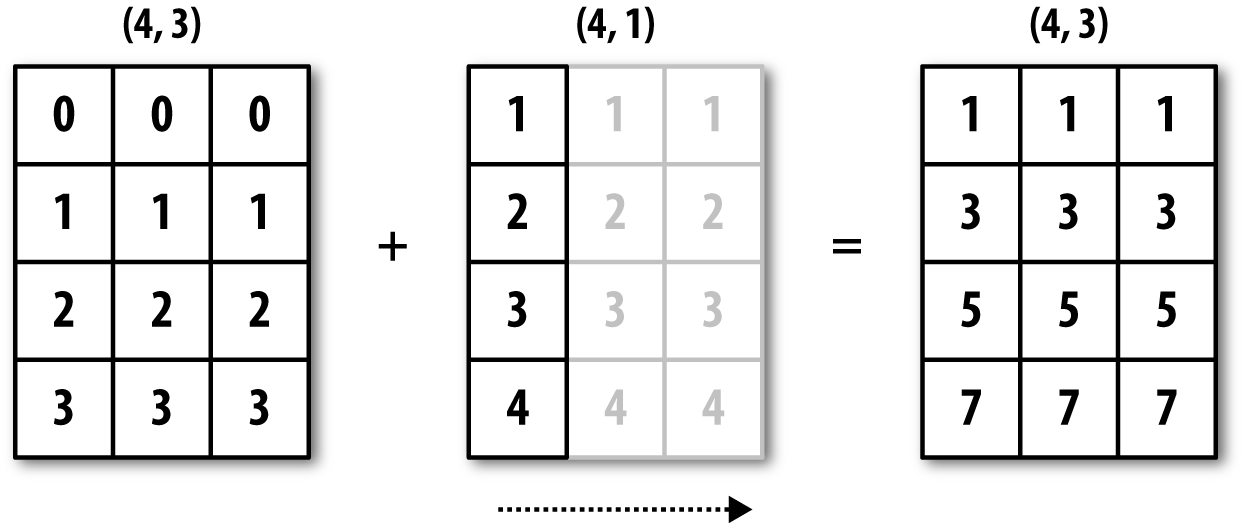
See Figure A-6 for another illustration, this time adding a two-dimensional array to a three-dimensional one across axis 0.
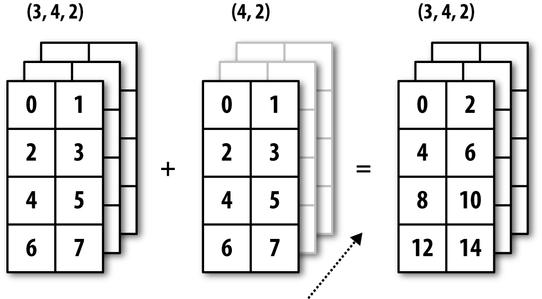
Broadcasting with higher dimensional arrays can seem even more mind-bending, but it is really a matter of following the rules. If you don’t, you’ll get an error like this:
In[93]:arr-arr.mean(1)---------------------------------------------------------------------------ValueErrorTraceback(mostrecentcalllast)<ipython-input-93-8b8ada26fac0>in<module>()---->1arr-arr.mean(1)ValueError:operandscouldnotbebroadcasttogetherwithshapes(4,3)(4,)
It’s quite common to want to perform an arithmetic operation with
a lower dimensional array across axes other than axis 0. According to
the broadcasting rule, the “broadcast dimensions” must be 1 in the
smaller array. In the example of row demeaning shown here, this meant
reshaping the row means to be shape (4,
1) instead of (4,):
In[94]:arr-arr.mean(1).reshape((4,1))Out[94]:array([[-0.2095,1.1334,-0.9239],[0.8562,-0.6828,-0.1734],[-0.3386,1.0823,-0.7438],[0.3234,-0.8599,0.5365]])
In the three-dimensional case, broadcasting over any of the three dimensions is only a matter of reshaping the data to be shape-compatible. Figure A-7 nicely visualizes the shapes required to broadcast over each axis of a three-dimensional array.
A common problem, therefore, is needing to add a new axis with
length 1 specifically for broadcasting purposes. Using reshape is one option, but inserting an axis
requires constructing a tuple indicating the new shape. This can often
be a tedious exercise. Thus, NumPy arrays offer a special syntax for
inserting new axes by indexing. We use the special np.newaxis
attribute along with “full” slices to insert the new axis:
In[95]:arr=np.zeros((4,4))In[96]:arr_3d=arr[:,np.newaxis,:]In[97]:arr_3d.shapeOut[97]:(4,1,4)In[98]:arr_1d=np.random.normal(size=3)In[99]:arr_1d[:,np.newaxis]Out[99]:array([[-2.3594],[-0.1995],[-1.542]])In[100]:arr_1d[np.newaxis,:]Out[100]:array([[-2.3594,-0.1995,-1.542]])
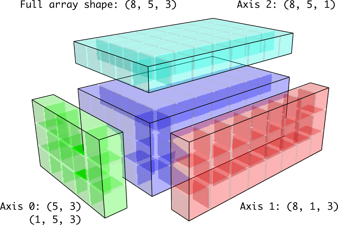
Thus, if we had a three-dimensional array and wanted to demean axis 2, say, we would need to write:
In[101]:arr=np.random.randn(3,4,5)In[102]:depth_means=arr.mean(2)In[103]:depth_meansOut[103]:array([[-0.4735,0.3971,-0.0228,0.2001],[-0.3521,-0.281,-0.071,-0.1586],[0.6245,0.6047,0.4396,-0.2846]])In[104]:depth_means.shapeOut[104]:(3,4)In[105]:demeaned=arr-depth_means[:,:,np.newaxis]In[106]:demeaned.mean(2)Out[106]:array([[0.,0.,-0.,-0.],[0.,0.,-0.,0.],[0.,0.,-0.,-0.]])
You might be wondering if there’s a way to generalize demeaning over an axis without sacrificing performance. There is, but it requires some indexing gymnastics:
defdemean_axis(arr,axis=0):means=arr.mean(axis)# This generalizes things like [:, :, np.newaxis] to N dimensionsindexer=[slice(None)]*arr.ndimindexer[axis]=np.newaxisreturnarr-means[indexer]
The same broadcasting rule governing arithmetic operations also applies to setting values via array indexing. In a simple case, we can do things like:
In[107]:arr=np.zeros((4,3))In[108]:arr[:]=5In[109]:arrOut[109]:array([[5.,5.,5.],[5.,5.,5.],[5.,5.,5.],[5.,5.,5.]])
However, if we had a one-dimensional array of values we wanted to set into the columns of the array, we can do that as long as the shape is compatible:
In[110]:col=np.array([1.28,-0.42,0.44,1.6])In[111]:arr[:]=col[:,np.newaxis]In[112]:arrOut[112]:array([[1.28,1.28,1.28],[-0.42,-0.42,-0.42],[0.44,0.44,0.44],[1.6,1.6,1.6]])In[113]:arr[:2]=[[-1.37],[0.509]]In[114]:arrOut[114]:array([[-1.37,-1.37,-1.37],[0.509,0.509,0.509],[0.44,0.44,0.44],[1.6,1.6,1.6]])
While many NumPy users will only make use of the fast element-wise operations provided by the universal functions, there are a number of additional features that occasionally can help you write more concise code without loops.
Each of NumPy’s binary ufuncs has special methods for performing certain kinds of special vectorized operations. These are summarized in Table A-2, but I’ll give a few concrete examples to illustrate how they work.
reduce takes a single array and aggregates its values, optionally along
an axis, by performing a sequence of binary operations. For example, an
alternative way to sum elements in an array is to use np.add.reduce:
In[115]:arr=np.arange(10)In[116]:np.add.reduce(arr)Out[116]:45In[117]:arr.sum()Out[117]:45
The starting value (0 for add)
depends on the ufunc. If an axis is passed, the reduction is performed
along that axis. This allows you to answer certain kinds of questions in
a concise way. As a less trivial example, we can use np.logical_and to check whether the values in each row of an array are
sorted:
In[118]:np.random.seed(12346)# for reproducibilityIn[119]:arr=np.random.randn(5,5)In[120]:arr[::2].sort(1)# sort a few rowsIn[121]:arr[:,:-1]<arr[:,1:]Out[121]:array([[True,True,True,True],[False,True,False,False],[True,True,True,True],[True,False,True,True],[True,True,True,True]],dtype=bool)In[122]:np.logical_and.reduce(arr[:,:-1]<arr[:,1:],axis=1)Out[122]:array([True,False,True,False,True],dtype=bool)
Note that logical_and.reduce is
equivalent to the all
method.
accumulate is related to reduce like
cumsum is related to sum. It produces an array of the same size
with the intermediate “accumulated” values:
In[123]:arr=np.arange(15).reshape((3,5))In[124]:np.add.accumulate(arr,axis=1)Out[124]:array([[0,1,3,6,10],[5,11,18,26,35],[10,21,33,46,60]])
outer performs a pairwise
cross-product between two arrays:
In[125]:arr=np.arange(3).repeat([1,2,2])In[126]:arrOut[126]:array([0,1,1,2,2])In[127]:np.multiply.outer(arr,np.arange(5))Out[127]:array([[0,0,0,0,0],[0,1,2,3,4],[0,1,2,3,4],[0,2,4,6,8],[0,2,4,6,8]])
The output of outer will have a
dimension that is the sum of the dimensions of the inputs:
In[128]:x,y=np.random.randn(3,4),np.random.randn(5)In[129]:result=np.subtract.outer(x,y)In[130]:result.shapeOut[130]:(3,4,5)
The last method, reduceat,
performs a “local reduce,” in essence an array
groupby operation in which slices of the array are
aggregated together. It accepts a sequence of “bin edges” that indicate
how to split and aggregate the values:
In[131]:arr=np.arange(10)In[132]:np.add.reduceat(arr,[0,5,8])Out[132]:array([10,18,17])
The results are the reductions (here, sums) performed over
arr[0:5], arr[5:8], and arr[8:]. As with the other methods, you can pass
an axis argument:
In[133]:arr=np.multiply.outer(np.arange(4),np.arange(5))In[134]:arrOut[134]:array([[0,0,0,0,0],[0,1,2,3,4],[0,2,4,6,8],[0,3,6,9,12]])In[135]:np.add.reduceat(arr,[0,2,4],axis=1)Out[135]:array([[0,0,0],[1,5,4],[2,10,8],[3,15,12]])
See Table A-2 for a partial listing of ufunc methods.
There are a number of facilities for creating your own NumPy ufuncs. The most general is to use the NumPy C API, but that is beyond the scope of this book. In this section, we will look at pure Python ufuncs.
numpy.frompyfunc accepts
a Python function along with a specification for the
number of inputs and outputs. For example, a simple function that adds
element-wise would be specified as:
In[136]:defadd_elements(x,y):.....:returnx+yIn[137]:add_them=np.frompyfunc(add_elements,2,1)In[138]:add_them(np.arange(8),np.arange(8))Out[138]:array([0,2,4,6,8,10,12,14],dtype=object)
Functions created using frompyfunc always return arrays of Python
objects, which can be inconvenient. Fortunately, there is an alternative
(but slightly less featureful) function, numpy.vectorize, that allows you to specify the output type:
In[139]:add_them=np.vectorize(add_elements,otypes=[np.float64])In[140]:add_them(np.arange(8),np.arange(8))Out[140]:array([0.,2.,4.,6.,8.,10.,12.,14.])
These functions provide a way to create ufunc-like functions, but they are very slow because they require a Python function call to compute each element, which is a lot slower than NumPy’s C-based ufunc loops:
In[141]:arr=np.random.randn(10000)In[142]:%timeitadd_them(arr,arr)3.54ms+-178usperloop(mean+-std.dev.of7runs,100loopseach)In[143]:%timeitnp.add(arr,arr)6.76us+-370nsperloop(mean+-std.dev.of7runs,100000loopseach)
Later in this chapter we’ll show how to create fast ufuncs in Python using the Numba project.
You may have noticed up until now that ndarray is a homogeneous data container; that is, it represents a block of memory in which each element takes up the same number of bytes, determined by the dtype. On the surface, this would appear to not allow you to represent heterogeneous or tabular-like data. A structured array is an ndarray in which each element can be thought of as representing a struct in C (hence the “structured” name) or a row in a SQL table with multiple named fields:
In[144]:dtype=[('x',np.float64),('y',np.int32)]In[145]:sarr=np.array([(1.5,6),(np.pi,-2)],dtype=dtype)In[146]:sarrOut[146]:array([(1.5,6),(3.1416,-2)],dtype=[('x','<f8'),('y','<i4')])
There are several ways to specify a structured dtype (see the online
NumPy documentation). One typical way is as a list of tuples with (field_name, field_data_type). Now, the elements
of the array are tuple-like objects whose elements can be accessed like a
dictionary:
In[147]:sarr[0]Out[147]:(1.5,6)In[148]:sarr[0]['y']Out[148]:6
The field names are stored in the dtype.names
attribute. When you access a field on the structured array, a strided view
on the data is returned, thus copying nothing:
In[149]:sarr['x']Out[149]:array([1.5,3.1416])
When specifying a structured dtype, you can additionally pass a shape (as an int or tuple):
In[150]:dtype=[('x',np.int64,3),('y',np.int32)]In[151]:arr=np.zeros(4,dtype=dtype)In[152]:arrOut[152]:array([([0,0,0],0),([0,0,0],0),([0,0,0],0),([0,0,0],0)],dtype=[('x','<i8',(3,)),('y','<i4')])
In this case, the x field now
refers to an array of length 3 for each record:
In[153]:arr[0]['x']Out[153]:array([0,0,0])
Conveniently, accessing arr['x'] then returns a two-dimensional array
instead of a one-dimensional array as in prior examples:
In[154]:arr['x']Out[154]:array([[0,0,0],[0,0,0],[0,0,0],[0,0,0]])
This enables you to express more complicated, nested structures as a single block of memory in an array. You can also nest dtypes to make more complex structures. Here is an example:
In[155]:dtype=[('x',[('a','f8'),('b','f4')]),('y',np.int32)]In[156]:data=np.array([((1,2),5),((3,4),6)],dtype=dtype)In[157]:data['x']Out[157]:array([(1.,2.),(3.,4.)],dtype=[('a','<f8'),('b','<f4')])In[158]:data['y']Out[158]:array([5,6],dtype=int32)In[159]:data['x']['a']Out[159]:array([1.,3.])
pandas DataFrame does not support this feature directly, though it is similar to hierarchical indexing.
Compared with, say, a pandas DataFrame, NumPy structured arrays are a comparatively low-level tool. They provide a means to interpreting a block of memory as a tabular structure with arbitrarily complex nested columns. Since each element in the array is represented in memory as a fixed number of bytes, structured arrays provide a very fast and efficient way of writing data to and from disk (including memory maps), transporting it over the network, and other such uses.
As another common use for structured arrays, writing data files as
fixed-length record byte streams is a common way to serialize data in C
and C++ code, which is commonly found in legacy systems in industry. As
long as the format of the file is known (the size of each record and the
order, byte size, and data type of each element), the data can be read
into memory with np.fromfile.
Specialized uses like this are beyond the scope of this book, but it’s
worth knowing that such things are possible.
Like Python’s built-in list, the ndarray sort instance
method is an in-place sort, meaning that the
array contents are rearranged without producing a new array:
In[160]:arr=np.random.randn(6)In[161]:arr.sort()In[162]:arrOut[162]:array([-1.082,0.3759,0.8014,1.1397,1.2888,1.8413])
When sorting arrays in-place, remember that if the array is a view on a different ndarray, the original array will be modified:
In[163]:arr=np.random.randn(3,5)In[164]:arrOut[164]:array([[-0.3318,-1.4711,0.8705,-0.0847,-1.1329],[-1.0111,-0.3436,2.1714,0.1234,-0.0189],[0.1773,0.7424,0.8548,1.038,-0.329]])In[165]:arr[:,0].sort()# Sort first column values in-placeIn[166]:arrOut[166]:array([[-1.0111,-1.4711,0.8705,-0.0847,-1.1329],[-0.3318,-0.3436,2.1714,0.1234,-0.0189],[0.1773,0.7424,0.8548,1.038,-0.329]])
On the other hand, numpy.sort
creates a new, sorted copy of an array. Otherwise, it accepts the same
arguments (such as kind) as ndarray.sort:
In[167]:arr=np.random.randn(5)In[168]:arrOut[168]:array([-1.1181,-0.2415,-2.0051,0.7379,-1.0614])In[169]:np.sort(arr)Out[169]:array([-2.0051,-1.1181,-1.0614,-0.2415,0.7379])In[170]:arrOut[170]:array([-1.1181,-0.2415,-2.0051,0.7379,-1.0614])
All of these sort methods take an axis argument for sorting the sections of data along the passed axis independently:
In[171]:arr=np.random.randn(3,5)In[172]:arrOut[172]:array([[0.5955,-0.2682,1.3389,-0.1872,0.9111],[-0.3215,1.0054,-0.5168,1.1925,-0.1989],[0.3969,-1.7638,0.6071,-0.2222,-0.2171]])In[173]:arr.sort(axis=1)In[174]:arrOut[174]:array([[-0.2682,-0.1872,0.5955,0.9111,1.3389],[-0.5168,-0.3215,-0.1989,1.0054,1.1925],[-1.7638,-0.2222,-0.2171,0.3969,0.6071]])
You may notice that none of the sort methods have an option to sort
in descending order. This is a problem in practice because array slicing
produces views, thus not producing a copy or requiring any computational
work. Many Python users are familiar with the “trick” that for a list
values, values[::-1] returns a list in reverse order.
The same is true for ndarrays:
In[175]:arr[:,::-1]Out[175]:array([[1.3389,0.9111,0.5955,-0.1872,-0.2682],[1.1925,1.0054,-0.1989,-0.3215,-0.5168],[0.6071,0.3969,-0.2171,-0.2222,-1.7638]])
In data analysis you may need to reorder datasets by one or more keys. For example, a table
of data about some students might need to be sorted by last name, then by
first name. This is an example of an indirect sort,
and if you’ve read the pandas-related chapters you have already seen
many higher-level examples. Given a key or keys (an array of values or
multiple arrays of values), you wish to obtain an array of integer
indices (I refer to them colloquially as
indexers) that tells you how to reorder the data to
be in sorted order. Two methods for this are argsort and numpy.lexsort. As an example:
In[176]:values=np.array([5,0,1,3,2])In[177]:indexer=values.argsort()In[178]:indexerOut[178]:array([1,2,4,3,0])In[179]:values[indexer]Out[179]:array([0,1,2,3,5])
As a more complicated example, this code reorders a two-dimensional array by its first row:
In[180]:arr=np.random.randn(3,5)In[181]:arr[0]=valuesIn[182]:arrOut[182]:array([[5.,0.,1.,3.,2.],[-0.3636,-0.1378,2.1777,-0.4728,0.8356],[-0.2089,0.2316,0.728,-1.3918,1.9956]])In[183]:arr[:,arr[0].argsort()]Out[183]:array([[0.,1.,2.,3.,5.],[-0.1378,2.1777,0.8356,-0.4728,-0.3636],[0.2316,0.728,1.9956,-1.3918,-0.2089]])
lexsort is similar to argsort, but it performs an indirect
lexicographical sort on multiple key arrays.
Suppose we wanted to sort some data identified by first and last
names:
In[184]:first_name=np.array(['Bob','Jane','Steve','Bill','Barbara'])In[185]:last_name=np.array(['Jones','Arnold','Arnold','Jones','Walters'])In[186]:sorter=np.lexsort((first_name,last_name))In[187]:sorterOut[187]:array([1,2,3,0,4])In[188]:zip(last_name[sorter],first_name[sorter])Out[188]:<zipat0x7efeec8e38c8>
lexsort can be a bit confusing
the first time you use it because the order in which the keys are used
to order the data starts with the last array
passed. Here, last_name was used
before first_name.
A stable sorting algorithm preserves the relative position of equal elements. This can be especially important in indirect sorts where the relative ordering is meaningful:
In[189]:values=np.array(['2:first','2:second','1:first','1:second',.....:'1:third'])In[190]:key=np.array([2,2,1,1,1])In[191]:indexer=key.argsort(kind='mergesort')In[192]:indexerOut[192]:array([2,3,4,0,1])In[193]:values.take(indexer)Out[193]:array(['1:first','1:second','1:third','2:first','2:second'],dtype='<U8')
The only stable sort available is mergesort, which has guaranteed
O(n log n) performance (for complexity buffs), but
its performance is on average worse than the default quicksort method. See Table A-3 for a summary of available methods
and their relative performance (and performance guarantees). This is not
something that most users will ever have to think about, but it’s useful to know that it’s there.
| Kind | Speed | Stable | Work space | Worst case |
|---|---|---|---|---|
'quicksort' | 1 | No | 0 | O(n^2) |
'mergesort' | 2 | Yes | n / 2 | O(n log n) |
'heapsort' | 3 | No | 0 | O(n log n) |
One of the goals of sorting can be to determine the largest or smallest elements in an
array. NumPy has optimized methods, numpy.partition
and np.argpartition, for partitioning an array around the k-th
smallest element:
In[194]:np.random.seed(12345)In[195]:arr=np.random.randn(20)In[196]:arrOut[196]:array([-0.2047,0.4789,-0.5194,-0.5557,1.9658,1.3934,0.0929,0.2817,0.769,1.2464,1.0072,-1.2962,0.275,0.2289,1.3529,0.8864,-2.0016,-0.3718,1.669,-0.4386])In[197]:np.partition(arr,3)Out[197]:array([-2.0016,-1.2962,-0.5557,-0.5194,-0.3718,-0.4386,-0.2047,0.2817,0.769,0.4789,1.0072,0.0929,0.275,0.2289,1.3529,0.8864,1.3934,1.9658,1.669,1.2464])
After you call partition(arr, 3), the first
three elements in the result are the smallest three values in no
particular order. numpy.argpartition, similar
to numpy.argsort, returns the indices
that rearrange the data into the equivalent order:
In[198]:indices=np.argpartition(arr,3)In[199]:indicesOut[199]:array([16,11,3,2,17,19,0,7,8,1,10,6,12,13,14,15,5,4,18,9])In[200]:arr.take(indices)Out[200]:array([-2.0016,-1.2962,-0.5557,-0.5194,-0.3718,-0.4386,-0.2047,0.2817,0.769,0.4789,1.0072,0.0929,0.275,0.2289,1.3529,0.8864,1.3934,1.9658,1.669,1.2464])
searchsorted is an array
method that performs a binary search on a sorted array,
returning the location in the array where the value would need to be
inserted to maintain sortedness:
In[201]:arr=np.array([0,1,7,12,15])In[202]:arr.searchsorted(9)Out[202]:3
You can also pass an array of values to get an array of indices back:
In[203]:arr.searchsorted([0,8,11,16])Out[203]:array([0,3,3,5])
You might have noticed that searchsorted returned 0 for the 0
element. This is because the default behavior is to return the index at
the left side of a group of equal values:
In[204]:arr=np.array([0,0,0,1,1,1,1])In[205]:arr.searchsorted([0,1])Out[205]:array([0,3])In[206]:arr.searchsorted([0,1],side='right')Out[206]:array([3,7])
As another application of searchsorted, suppose we had an array of
values between 0 and 10,000, and a separate array of “bucket edges” that
we wanted to use to bin the data:
In[207]:data=np.floor(np.random.uniform(0,10000,size=50))In[208]:bins=np.array([0,100,1000,5000,10000])In[209]:dataOut[209]:array([9940.,6768.,7908.,1709.,268.,8003.,9037.,246.,4917.,5262.,5963.,519.,8950.,7282.,8183.,5002.,8101.,959.,2189.,2587.,4681.,4593.,7095.,1780.,5314.,1677.,7688.,9281.,6094.,1501.,4896.,3773.,8486.,9110.,3838.,3154.,5683.,1878.,1258.,6875.,7996.,5735.,9732.,6340.,8884.,4954.,3516.,7142.,5039.,2256.])
To then get a labeling of which interval each data point belongs
to (where 1 would mean the bucket [0,
100)), we can simply use searchsorted:
In[210]:labels=bins.searchsorted(data)In[211]:labelsOut[211]:array([4,4,4,3,2,4,4,2,3,4,4,2,4,4,4,4,4,2,3,3,3,3,4,3,4,3,4,4,4,3,3,3,4,4,3,3,4,3,3,4,4,4,4,4,4,3,3,4,4,3])
This, combined with pandas’s groupby, can be used to bin data:
In[212]:pd.Series(data).groupby(labels).mean()Out[212]:2498.00000033064.27777847389.035714dtype:float64
Numba is an open source project that creates fast functions for NumPy-like data using CPUs, GPUs, or other hardware. It uses the LLVM Project to translate Python code into compiled machine code.
To introduce Numba, let’s consider a pure Python function that
computes the expression (x - y).mean() using a
for loop:
importnumpyasnpdefmean_distance(x,y):nx=len(x)result=0.0count=0foriinrange(nx):result+=x[i]-y[i]count+=1returnresult/count
This function is very slow:
In[209]:x=np.random.randn(10000000)In[210]:y=np.random.randn(10000000)In[211]:%timeitmean_distance(x,y)1loop,bestof3:2sperloopIn[212]:%timeit(x-y).mean()100loops,bestof3:14.7msperloop
The NumPy version is over 100 times faster. We can turn this
function into a compiled Numba function using the numba.jit function:
In[213]:importnumbaasnbIn[214]:numba_mean_distance=nb.jit(mean_distance)
We could also have written this as a decorator:
@nb.jitdefmean_distance(x,y):nx=len(x)result=0.0count=0foriinrange(nx):result+=x[i]-y[i]count+=1returnresult/count
The resulting function is actually faster than the vectorized NumPy version:
In[215]:%timeitnumba_mean_distance(x,y)100loops,bestof3:10.3msperloop
Numba cannot compile arbitrary Python code, but it supports a significant subset of pure Python that is most useful for writing numerical algorithms.
Numba is a deep library, supporting different kinds of hardware,
modes of compilation, and user extensions. It is also able to compile a
substantial subset of the NumPy Python API without explicit
for loops. Numba is able to recognize constructs that
can be compiled to machine code, while substituting calls to the CPython
API for functions that it does not know how to compile. Numba’s
jit function has an option, nopython=True, which
restricts allowed code to Python code that can be compiled to LLVM without
any Python C API calls. jit(nopython=True) has a
shorter alias numba.njit.
In the previous example, we could have written:
fromnumbaimportfloat64,njit@njit(float64(float64[:],float64[:]))defmean_distance(x,y):return(x-y).mean()
I encourage you to learn more by reading the online documentation for Numba. The next section shows an example of creating custom NumPy ufunc objects.
The numba.vectorize function creates compiled NumPy ufuncs, which behave like built-in
ufuncs. Let’s consider a Python implementation of
numpy.add:
fromnumbaimportvectorize@vectorizedefnb_add(x,y):returnx+y
In[13]:x=np.arange(10)In[14]:nb_add(x,x)Out[14]:array([0.,2.,4.,6.,8.,10.,12.,14.,16.,18.])In[15]:nb_add.accumulate(x,0)Out[15]:array([0.,1.,3.,6.,10.,15.,21.,28.,36.,45.])
In Chapter 4, we became acquainted with np.save and np.load for storing arrays in binary format on
disk. There are a number of additional options to consider for more
sophisticated use. In particular, memory maps have the additional benefit
of enabling you to work with datasets that do not fit into RAM.
A memory-mapped file is a method for interacting with binary data on disk as
though it is stored in an in-memory array. NumPy implements a memmap object that is ndarray-like, enabling small segments of a large
file to be read and written without reading the whole array into memory.
Additionally, a memmap has the same methods as an
in-memory array and thus can be substituted into many algorithms where
an ndarray would be expected.
To create a new memory map, use the function np.memmap and pass a file path, dtype, shape,
and file mode:
In[214]:mmap=np.memmap('mymmap',dtype='float64',mode='w+',.....:shape=(10000,10000))In[215]:mmapOut[215]:memmap([[0.,0.,0.,...,0.,0.,0.],[0.,0.,0.,...,0.,0.,0.],[0.,0.,0.,...,0.,0.,0.],...,[0.,0.,0.,...,0.,0.,0.],[0.,0.,0.,...,0.,0.,0.],[0.,0.,0.,...,0.,0.,0.]])
Slicing a memmap returns views on the data on
disk:
In[216]:section=mmap[:5]
If you assign data to these, it will be buffered in memory (like a
Python file object), but you can write it to disk by calling flush:
In[217]:section[:]=np.random.randn(5,10000)In[218]:mmap.flush()In[219]:mmapOut[219]:memmap([[0.7584,-0.6605,0.8626,...,0.6046,-0.6212,2.0542],[-1.2113,-1.0375,0.7093,...,-1.4117,-0.1719,-0.8957],[-0.1419,-0.3375,0.4329,...,1.2914,-0.752,-0.44],...,[0.,0.,0.,...,0.,0.,0.],[0.,0.,0.,...,0.,0.,0.],[0.,0.,0.,...,0.,0.,0.]])In[220]:delmmap
Whenever a memory map falls out of scope and is garbage-collected, any changes will be flushed to disk also. When opening an existing memory map, you still have to specify the dtype and shape, as the file is only a block of binary data with no metadata on disk:
In[221]:mmap=np.memmap('mymmap',dtype='float64',shape=(10000,10000))In[222]:mmapOut[222]:memmap([[0.7584,-0.6605,0.8626,...,0.6046,-0.6212,2.0542],[-1.2113,-1.0375,0.7093,...,-1.4117,-0.1719,-0.8957],[-0.1419,-0.3375,0.4329,...,1.2914,-0.752,-0.44],...,[0.,0.,0.,...,0.,0.,0.],[0.,0.,0.,...,0.,0.,0.],[0.,0.,0.,...,0.,0.,0.]])
Memory maps also work with structured or nested dtypes as described in a previous section.
PyTables and h5py are two Python projects providing NumPy-friendly interfaces for storing array data in the efficient and compressible HDF5 format (HDF stands for hierarchical data format). You can safely store hundreds of gigabytes or even terabytes of data in HDF5 format. To learn more about using HDF5 with Python, I recommend reading the pandas online documentation.
Getting good performance out of code utilizing NumPy is often straightforward, as array operations typically replace otherwise comparatively extremely slow pure Python loops. The following list briefly summarizes some things to keep in mind:
Convert Python loops and conditional logic to array operations and boolean array operations
Use broadcasting whenever possible
Use arrays views (slicing) to avoid copying data
Utilize ufuncs and ufunc methods
If you can’t get the performance you require after exhausting the capabilities provided by NumPy alone, consider writing code in C, Fortran, or Cython. I use Cython frequently in my own work as an easy way to get C-like performance with minimal development.
While the full extent of this topic is a bit outside the scope of this book, in some applications the memory layout of an array can significantly affect the speed of computations. This is based partly on performance differences having to do with the cache hierarchy of the CPU; operations accessing contiguous blocks of memory (e.g., summing the rows of a C order array) will generally be the fastest because the memory subsystem will buffer the appropriate blocks of memory into the ultrafast L1 or L2 CPU cache. Also, certain code paths inside NumPy’s C codebase have been optimized for the contiguous case in which generic strided memory access can be avoided.
To say that an array’s memory layout is
contiguous means that the elements are stored in
memory in the order that they appear in the array with respect to
Fortran (column major) or C (row major) ordering. By
default, NumPy arrays are created as C-contiguous
or just simply contiguous. A column major array, such as the transpose
of a C-contiguous array, is thus said to be Fortran-contiguous. These
properties can be explicitly checked via the flags attribute on the ndarray:
In[225]:arr_c=np.ones((1000,1000),order='C')In[226]:arr_f=np.ones((1000,1000),order='F')In[227]:arr_c.flagsOut[227]:C_CONTIGUOUS:TrueF_CONTIGUOUS:FalseOWNDATA:TrueWRITEABLE:TrueALIGNED:TrueUPDATEIFCOPY:FalseIn[228]:arr_f.flagsOut[228]:C_CONTIGUOUS:FalseF_CONTIGUOUS:TrueOWNDATA:TrueWRITEABLE:TrueALIGNED:TrueUPDATEIFCOPY:FalseIn[229]:arr_f.flags.f_contiguousOut[229]:True
In this example, summing the rows of these arrays should, in
theory, be faster for arr_c than
arr_f since the rows are contiguous
in memory. Here I check for sure using %timeit in
IPython:
In[230]:%timeitarr_c.sum(1)842us+-40.3usperloop(mean+-std.dev.of7runs,1000loopseach)In[231]:%timeitarr_f.sum(1)879us+-23.6usperloop(mean+-std.dev.of7runs,1000loopseach)
When you’re looking to squeeze more performance out of NumPy, this is
often a place to invest some effort. If you have an array that does not
have the desired memory order, you can use copy and pass either 'C' or 'F':
In[232]:arr_f.copy('C').flagsOut[232]:C_CONTIGUOUS:TrueF_CONTIGUOUS:FalseOWNDATA:TrueWRITEABLE:TrueALIGNED:TrueUPDATEIFCOPY:False
When constructing a view on an array, keep in mind that the result is not guaranteed to be contiguous:
In[233]:arr_c[:50].flags.contiguousOut[233]:TrueIn[234]:arr_c[:,:50].flagsOut[234]:C_CONTIGUOUS:FalseF_CONTIGUOUS:FalseOWNDATA:FalseWRITEABLE:TrueALIGNED:TrueUPDATEIFCOPY:False
1 Some of the dtypes have trailing underscores in their names. These are there to avoid variable name conflicts between the NumPy-specific types and the Python built-in ones.
In Chapter 2 we looked at the basics of using the IPython shell and Jupyter notebook. In this chapter, we explore some deeper functionality in the IPython system that can either be used from the console or within Jupyter.
IPython maintains a small on-disk database containing the text of each command that you execute. This serves various purposes:
Searching, completing, and executing previously executed commands with minimal typing
Persisting the command history between sessions
Logging the input/output history to a file
These features are more useful in the shell than in the notebook, since the notebook by design keeps a log of the input and output in each code cell.
The IPython shell lets you search and execute previous code or other commands.
This is useful, as you may often find yourself repeating the same
commands, such as a %run command or some
other code snippet. Suppose you had run:
In[7]: %run first/second/third/data_script.py
and then explored the results of the script (assuming it ran
successfully) only to find that you made an incorrect calculation. After
figuring out the problem and modifying
data_script.py, you can start typing a few letters
of the %run command and then press either
the Ctrl-P key combination or the up arrow key. This will
search the command history for the first prior command matching the
letters you typed. Pressing either Ctrl-P or the up arrow key multiple
times will continue to search through the history. If you pass over the
command you wish to execute, fear not. You can move
forward through the command history by pressing
either Ctrl-N or the down arrow key. After doing this a few times,
you may start pressing these keys without thinking!
Using Ctrl-R gives you the same partial incremental searching capability
provided by the readline used in
Unix-style shells, such as the bash shell. On Windows, readline functionality is emulated by IPython. To use this, press Ctrl-R and then
type a few characters contained in the input line you want to search
for:
In [1]: a_command = foo(x, y, z) (reverse-i-search)`com': a_command = foo(x, y, z)
Pressing Ctrl-R will cycle through the history for each line matching the characters you’ve typed.
Forgetting to assign the result of a function call to a variable can be very
annoying. An IPython session stores references to
both the input commands and output Python objects
in special variables. The previous two outputs are stored in the _ (one underscore)
and __ (two underscores) variables,
respectively:
In[24]:2**27Out[24]:134217728In[25]:_Out[25]:134217728
Input variables are stored in variables named like _iX, where X is the input line number. For each input
variable there is a corresponding output variable _X. So after input line 27, say, there will be
two new variables _27 (for the
output) and _i27 for the
input:
In[26]:foo='bar'In[27]:fooOut[27]:'bar'In[28]:_i27Out[28]:u'foo'In[29]:_27Out[29]:'bar'
Since the input variables are strings they can be executed again
with the Python exec keyword:
In[30]:exec(_i27)
Here _i27 refers to the code input in
In [27].
Several magic functions allow you to work with the input and
output history. %hist is capable of
printing all or part of the input history, with or without line numbers.
%reset is for clearing the
interactive namespace and optionally the input and output caches. The
%xdel magic function is intended for
removing all references to a particular object from
the IPython machinery. See the documentation for both of these magics
for more details.
When working with very large datasets, keep in mind that
IPython’s input and output history causes any object referenced there
to not be garbage-collected (freeing up the memory), even if you
delete the variables from the interactive namespace using the del keyword. In such cases, careful usage
of %xdel and %reset can help you avoid running into memory problems.
Another feature of IPython is that it allows you to seamlessly access the filesystem and operating system shell. This means, among other things, that you can perform most standard command-line actions as you would in the Windows or Unix (Linux, macOS) shell without having to exit IPython. This includes shell commands, changing directories, and storing the results of a command in a Python object (list or string). There are also simple command aliasing and directory bookmarking features.
See Table B-1 for a summary of magic functions and syntax for calling shell commands. I’ll briefly visit these features in the next few sections.
Starting a line in IPython with an exclamation point !, or bang, tells IPython to execute
everything after the bang in the system shell. This means that you can
delete files (using rm or del, depending on your OS), change
directories, or execute any other process.
You can store the console output of a shell command in a
variable by assigning the expression escaped with
! to a variable. For example, on my Linux-based
machine connected to the internet via ethernet, I can get my IP address
as a Python variable:
In[1]:ip_info=!ifconfigwlan0|grep"inet "In[2]:ip_info[0].strip()Out[2]:'inet addr:10.0.0.11 Bcast:10.0.0.255 Mask:255.255.255.0'
The returned Python object ip_info is actually a custom list type
containing various versions of the console output.
IPython can also substitute in Python values defined in the
current environment when using !. To
do this, preface the variable name by the dollar sign $:
In[3]:foo='test*'In[4]:!ls$footest4.pytest.pytest.xml
The %alias magic function can define custom shortcuts for shell commands.
As a simple example:
In[1]:%aliasllls-lIn[2]:ll/usrtotal332drwxr-xr-x2rootroot696322012-01-2920:36bin/drwxr-xr-x2rootroot40962010-08-2312:05games/drwxr-xr-x123rootroot204802011-12-2618:08include/drwxr-xr-x265rootroot1269762012-01-2920:36lib/drwxr-xr-x44rootroot696322011-12-2618:08lib32/lrwxrwxrwx1rootroot32010-08-2316:02lib64->lib/drwxr-xr-x15rootroot40962011-10-1319:03local/drwxr-xr-x2rootroot122882012-01-1209:32sbin/drwxr-xr-x387rootroot122882011-11-0422:53share/drwxrwsr-x24rootsrc40962011-07-1718:38src/
You can execute multiple commands just as on the command line by separating them with semicolons:
In[558]:%aliastest_alias(cdexamples;ls;cd..)In[559]:test_aliasmacrodata.csvspx.csvtips.csv
You’ll notice that IPython “forgets” any aliases you define interactively as soon as the session is closed. To create permanent aliases, you will need to use the configuration system.
IPython has a simple directory bookmarking system to enable you to save aliases for common directories so that you can jump around very easily. For example, suppose you wanted to create a bookmark that points to the supplementary materials for this book:
In[6]:%bookmarkpy4da/home/wesm/code/pydata-book
Once you’ve done this, when we use the %cd magic, we can
use any bookmarks we’ve defined:
In[7]:cdpy4da(bookmark:py4da)->/home/wesm/code/pydata-book/home/wesm/code/pydata-book
If a bookmark name conflicts with a directory name in your current
working directory, you can use the -b
flag to override and use the bookmark location. Using the -l option with %bookmark lists
all of your bookmarks:
In[8]:%bookmark-lCurrentbookmarks:py4da->/home/wesm/code/pydata-book-source
Bookmarks, unlike aliases, are automatically persisted between IPython sessions.
In addition to being a comfortable environment for interactive computing and data
exploration, IPython can also be a useful companion for general Python
software development. In data analysis applications, it’s important first
to have correct code. Fortunately, IPython has
closely integrated and enhanced the built-in Python pdb debugger. Secondly you want your code to be
fast. For this IPython has easy-to-use code timing
and profiling tools. I will give an overview of these tools in detail
here.
IPython’s debugger enhances pdb with tab
completion, syntax highlighting, and context for each line in exception
tracebacks. One of the best times to debug code is right after an error
has occurred. The %debug command,
when entered immediately after an exception, invokes the “post-mortem”
debugger and drops you into the stack frame where the exception was
raised:
In[2]:runexamples/ipython_bug.py---------------------------------------------------------------------------AssertionErrorTraceback(mostrecentcalllast)/home/wesm/code/pydata-book/examples/ipython_bug.pyin<module>()13throws_an_exception()14--->15calling_things()/home/wesm/code/pydata-book/examples/ipython_bug.pyincalling_things()11defcalling_things():12works_fine()--->13throws_an_exception()1415calling_things()/home/wesm/code/pydata-book/examples/ipython_bug.pyinthrows_an_exception()7a=58b=6---->9assert(a+b==10)1011defcalling_things():AssertionError:In[3]:%debug>/home/wesm/code/pydata-book/examples/ipython_bug.py(9)throws_an_exception()8b=6---->9assert(a+b==10)10ipdb>
Once inside the debugger, you can execute arbitrary Python code
and explore all of the objects and data (which have been “kept alive” by
the interpreter) inside each stack frame. By default you start in the
lowest level, where the error occurred. By pressing u (up) and d (down), you can switch between the levels of
the stack trace:
ipdb>u>/home/wesm/code/pydata-book/examples/ipython_bug.py(13)calling_things()12works_fine()--->13throws_an_exception()14
Executing the %pdb command
makes it so that IPython automatically invokes the
debugger after any exception, a mode that many users will find
especially useful.
It’s also easy to use the debugger to help develop code,
especially when you wish to set breakpoints or step through the
execution of a function or script to examine the state at each stage.
There are several ways to accomplish this. The first is by using %run with the
-d flag, which invokes the debugger
before executing any code in the passed script. You must immediately
press s (step) to enter the
script:
In[5]:run-dexamples/ipython_bug.pyBreakpoint1at/home/wesm/code/pydata-book/examples/ipython_bug.py:1NOTE:Enter'c'attheipdb>prompttostartyourscript.><string>(1)<module>()ipdb>s--Call-->/home/wesm/code/pydata-book/examples/ipython_bug.py(1)<module>()1--->1defworks_fine():2a=53b=6
After this point, it’s up to you how you want to work your way
through the file. For example, in the preceding exception, we could set
a breakpoint right before calling the works_fine method and run the script until we
reach the breakpoint by pressing c
(continue):
ipdb>b12ipdb>c>/home/wesm/code/pydata-book/examples/ipython_bug.py(12)calling_things()11defcalling_things():2-->12works_fine()13throws_an_exception()
At this point, you can step
into works_fine() or execute works_fine() by pressing n (next) to advance to the next line:
ipdb>n>/home/wesm/code/pydata-book/examples/ipython_bug.py(13)calling_things()212works_fine()--->13throws_an_exception()14
Then, we could step into throws_an_exception and advance to the line
where the error occurs and look at the variables in the scope. Note that
debugger commands take precedence over variable names; in such cases,
preface the variables with ! to
examine their contents:
ipdb>s--Call-->/home/wesm/code/pydata-book/examples/ipython_bug.py(6)throws_an_exception()5---->6defthrows_an_exception():7a=5ipdb>n>/home/wesm/code/pydata-book/examples/ipython_bug.py(7)throws_an_exception()6defthrows_an_exception():---->7a=58b=6ipdb>n>/home/wesm/code/pydata-book/examples/ipython_bug.py(8)throws_an_exception()7a=5---->8b=69assert(a+b==10)ipdb>n>/home/wesm/code/pydata-book/examples/ipython_bug.py(9)throws_an_exception()8b=6---->9assert(a+b==10)10ipdb>!a5ipdb>!b6
Developing proficiency with the interactive debugger is largely a matter of practice and experience. See Table B-2 for a full catalog of the debugger commands. If you are accustomed to using an IDE, you might find the terminal-driven debugger to be a bit unforgiving at first, but that will improve in time. Some of the Python IDEs have excellent GUI debuggers, so most users can find something that works for them.
There are a couple of other useful ways to invoke the debugger.
The first is by using a special set_trace function (named after pdb.set_trace), which is basically a “poor
man’s breakpoint.” Here are two small recipes you might want to put
somewhere for your general use (potentially adding them to your
IPython profile as I do):
fromIPython.core.debuggerimportPdbdefset_trace():Pdb(color_scheme='Linux').set_trace(sys._getframe().f_back)defdebug(f,*args,**kwargs):pdb=Pdb(color_scheme='Linux')returnpdb.runcall(f,*args,**kwargs)
The first function, set_trace, is very simple. You can use a
set_trace in any part of your
code that you want to temporarily stop in order to more closely
examine it (e.g., right before an exception occurs):
In[7]:runexamples/ipython_bug.py>/home/wesm/code/pydata-book/examples/ipython_bug.py(16)calling_things()15set_trace()--->16throws_an_exception()17
Pressing c (continue) will
cause the code to resume normally with no harm done.
The debug function we just looked at enables you to invoke the interactive
debugger easily on an arbitrary function call. Suppose we had written
a function like the following and we wished to step through its
logic:
deff(x,y,z=1):tmp=x+yreturntmp/z
Ordinarily using f would look
like f(1, 2, z=3). To instead step
into f, pass f as the first argument to debug followed by the positional and keyword
arguments to be passed to f:
In[6]:debug(f,1,2,z=3)><ipython-input>(2)f()1deff(x,y,z):---->2tmp=x+y3returntmp/zipdb>
I find that these two simple recipes save me a lot of time on a day-to-day basis.
Lastly, the debugger can be used in conjunction with %run. By running
a script with %run -d, you will be
dropped directly into the debugger, ready to set any breakpoints and
start the script:
In[1]:%run-dexamples/ipython_bug.pyBreakpoint1at/home/wesm/code/pydata-book/examples/ipython_bug.py:1NOTE:Enter'c'attheipdb>prompttostartyourscript.><string>(1)<module>()ipdb>
Adding -b with a line number
starts the debugger with a breakpoint set already:
In[2]:%run-d-b2examples/ipython_bug.pyBreakpoint1at/home/wesm/code/pydata-book/examples/ipython_bug.py:2NOTE:Enter'c'attheipdb>prompttostartyourscript.><string>(1)<module>()ipdb>c>/home/wesm/code/pydata-book/examples/ipython_bug.py(2)works_fine()1defworks_fine():1--->2a=53b=6ipdb>
For larger-scale or longer-running data analysis applications, you may wish to measure the execution time of various components or of individual statements or function calls. You may want a report of which functions are taking up the most time in a complex process. Fortunately, IPython enables you to get this information very easily while you are developing and testing your code.
Timing code by hand using the built-in time module and its functions time.clock and time.time is often tedious and repetitive, as
you must write the same uninteresting boilerplate code:
importtimestart=time.time()foriinrange(iterations):# some code to run hereelapsed_per=(time.time()-start)/iterations
Since this is such a common operation, IPython has two magic
functions, %time and
%timeit, to automate this process for you.
%time runs a statement once,
reporting the total execution time. Suppose we had a large list of
strings and we wanted to compare different methods of selecting all
strings starting with a particular prefix. Here is a simple list of
600,000 strings and two identical methods of selecting only the ones
that start with 'foo':
# a very large list of stringsstrings=['foo','foobar','baz','qux','python','Guido Van Rossum']*100000method1=[xforxinstringsifx.startswith('foo')]method2=[xforxinstringsifx[:3]=='foo']
It looks like they should be about the same performance-wise,
right? We can check for sure using %time:
In[561]:%timemethod1=[xforxinstringsifx.startswith('foo')]CPUtimes:user0.19s,sys:0.00s,total:0.19sWalltime:0.19sIn[562]:%timemethod2=[xforxinstringsifx[:3]=='foo']CPUtimes:user0.09s,sys:0.00s,total:0.09sWalltime:0.09s
The Wall time (short for
“wall-clock time”) is the main number of interest. So, it looks like the
first method takes more than twice as long, but it’s not a very precise
measurement. If you try %time-ing
those statements multiple times yourself, you’ll find that the results
are somewhat variable. To get a more precise measurement, use the
%timeit magic function. Given an
arbitrary statement, it has a heuristic to run a statement multiple
times to produce a more accurate average runtime:
In[563]:%timeit[xforxinstringsifx.startswith('foo')]10loops,bestof3:159msperloopIn[564]:%timeit[xforxinstringsifx[:3]=='foo']10loops,bestof3:59.3msperloop
This seemingly innocuous example illustrates that it is worth understanding the performance characteristics of the Python standard library, NumPy, pandas, and other libraries used in this book. In larger-scale data analysis applications, those milliseconds will start to add up!
%timeit is especially useful
for analyzing statements and functions with very short execution times,
even at the level of microseconds (millionths of a second) or
nanoseconds (billionths of a second). These may seem like insignificant
amounts of time, but of course a 20 microsecond function invoked 1
million times takes 15 seconds longer than a 5 microsecond function. In
the preceding example, we could very directly compare the two string
operations to understand their performance characteristics:
In[565]:x='foobar'In[566]:y='foo'In[567]:%timeitx.startswith(y)1000000loops,bestof3:267nsperloopIn[568]:%timeitx[:3]==y10000000loops,bestof3:147nsperloop
Profiling code is closely related to timing code, except it is concerned
with determining where time is spent. The main
Python profiling tool is the cProfile
module, which is not specific to IPython at all. cProfile executes a program or any arbitrary
block of code while keeping track of how much time is spent in each
function.
A common way to use cProfile is
on the command line, running an entire program and outputting the
aggregated time per function. Suppose we had a simple script that does
some linear algebra in a loop (computing the maximum absolute
eigenvalues of a series of 100 × 100 matrices):
importnumpyasnpfromnumpy.linalgimporteigvalsdefrun_experiment(niter=100):K=100results=[]for_inxrange(niter):mat=np.random.randn(K,K)max_eigenvalue=np.abs(eigvals(mat)).max()results.append(max_eigenvalue)returnresultssome_results=run_experiment()'Largest one we saw:%s'%np.max(some_results)
You can run this script through cProfile using the following in the command
line:
python -m cProfile cprof_example.py
If you try that, you’ll find that the output is sorted by function
name. This makes it a bit hard to get an idea of where the most time is
spent, so it’s very common to specify a sort order
using the -s flag:
$python-mcProfile-scumulativecprof_example.pyLargestonewesaw:11.92320442215116functioncalls(14927primitivecalls)in0.720secondsOrderedby:cumulativetimencallstottimepercallcumtimepercallfilename:lineno(function)10.0010.0010.7210.721cprof_example.py:1(<module>)1000.0030.0000.5860.006linalg.py:702(eigvals)2000.5720.0030.5720.003{numpy.linalg.lapack_lite.dgeev}10.0020.0020.0750.075__init__.py:106(<module>)1000.0590.0010.0590.001{method'randn')10.0000.0000.0440.044add_newdocs.py:9(<module>)20.0010.0010.0370.019__init__.py:1(<module>)20.0030.0020.0300.015__init__.py:2(<module>)10.0000.0000.0300.030type_check.py:3(<module>)10.0010.0010.0210.021__init__.py:15(<module>)10.0130.0130.0130.013numeric.py:1(<module>)10.0000.0000.0090.009__init__.py:6(<module>)10.0010.0010.0080.008__init__.py:45(<module>)2620.0050.0000.0070.000function_base.py:3178(add_newdoc)1000.0030.0000.0050.000linalg.py:162(_assertFinite)...
Only the first 15 rows of the output are shown. It’s easiest to
read by scanning down the cumtime
column to see how much total time was spent inside
each function. Note that if a function calls some other function,
the clock does not stop running. cProfile records the start and end time of
each function call and uses that to produce the timing.
In addition to the command-line usage, cProfile can also be used programmatically to
profile arbitrary blocks of code without having to run a new process.
IPython has a convenient interface to this capability using the %prun command
and the -p option to %run. %prun
takes the same “command-line options” as cProfile but will profile an arbitrary Python
statement instead of a whole .py file:
In[4]:%prun-l7-scumulativerun_experiment()4203functioncallsin0.643secondsOrderedby:cumulativetimeListreducedfrom32to7duetorestriction<7>ncallstottimepercallcumtimepercallfilename:lineno(function)10.0000.0000.6430.643<string>:1(<module>)10.0010.0010.6430.643cprof_example.py:4(run_experiment)1000.0030.0000.5830.006linalg.py:702(eigvals)2000.5690.0030.5690.003{numpy.linalg.lapack_lite.dgeev}1000.0580.0010.0580.001{method'randn'}1000.0030.0000.0050.000linalg.py:162(_assertFinite)2000.0020.0000.0020.000{method'all'of'numpy.ndarray'}
Similarly, calling %run -p -s cumulative
cprof_example.py has the same effect as the command-line
approach, except you never have to leave IPython.
In the Jupyter notebook, you can use the %%prun magic (two
% signs) to profile an entire code block. This pops
up a separate window with the profile output. This can be useful in
getting possibly quick answers to questions like, “Why did that code
block take so long to run?”
There are other tools available that help make profiles easier to understand when you are using IPython or Jupyter. One of these is SnakeViz, which produces an interactive visualization of the profile results using d3.js.
In some cases the information you obtain from %prun (or another cProfile-based profile method) may not tell
the whole story about a function’s execution time, or it may be so
complex that the results, aggregated by function name, are hard to
interpret. For this case, there is a small library called line_profiler (obtainable via PyPI or one of
the package management tools). It contains an IPython extension enabling
a new magic function %lprun that
computes a line-by-line-profiling of one or more functions. You can
enable this extension by modifying your IPython configuration (see the
IPython documentation or the section on configuration later in this
chapter) to include the following line:
# A list of dotted module names of IPython extensions to load.c.TerminalIPythonApp.extensions=['line_profiler']
You can also run the command:
%load_ext line_profiler
line_profiler can be used
programmatically (see the full documentation), but it is perhaps most
powerful when used interactively in IPython. Suppose you had a module
prof_mod with the following code
doing some NumPy array operations:
fromnumpy.randomimportrandndefadd_and_sum(x,y):added=x+ysummed=added.sum(axis=1)returnsummeddefcall_function():x=randn(1000,1000)y=randn(1000,1000)returnadd_and_sum(x,y)
If we wanted to understand the performance of the add_and_sum function, %prun gives us the following:
In[569]:%runprof_modIn[570]:x=randn(3000,3000)In[571]:y=randn(3000,3000)In[572]:%prunadd_and_sum(x,y)4functioncallsin0.049secondsOrderedby:internaltimencallstottimepercallcumtimepercallfilename:lineno(function)10.0360.0360.0460.046prof_mod.py:3(add_and_sum)10.0090.0090.0090.009{method'sum'of'numpy.ndarray'}10.0030.0030.0490.049<string>:1(<module>)
This is not especially enlightening. With the line_profiler IPython extension activated, a
new command %lprun is available. The
only difference in usage is that we must instruct %lprun which function or functions we wish to
profile. The general syntax is:
%lprun -f func1 -f func2 statement_to_profileIn this case, we want to profile add_and_sum, so we run:
In[573]:%lprun-fadd_and_sumadd_and_sum(x,y)Timerunit:1e-06sFile:prof_mod.pyFunction:add_and_sumatline3Totaltime:0.045936sLine# Hits Time Per Hit % Time Line Contents==============================================================3defadd_and_sum(x,y):413651036510.079.5added=x+y5194259425.020.5summed=added.sum(axis=1)6111.00.0returnsummed
This can be much easier to interpret. In this case we profiled the
same function we used in the statement. Looking at the preceding module
code, we could call call_function and
profile that as well as add_and_sum,
thus getting a full picture of the performance of the code:
In[574]:%lprun-fadd_and_sum-fcall_functioncall_function()Timerunit:1e-06sFile:prof_mod.pyFunction:add_and_sumatline3Totaltime:0.005526sLine# Hits Time Per Hit % Time Line Contents==============================================================3defadd_and_sum(x,y):4143754375.079.2added=x+y5111491149.020.8summed=added.sum(axis=1)6122.00.0returnsummedFile:prof_mod.pyFunction:call_functionatline8Totaltime:0.121016sLine# Hits Time Per Hit % Time Line Contents==============================================================8defcall_function():915716957169.047.2x=randn(1000,1000)1015830458304.048.2y=randn(1000,1000)11155435543.04.6returnadd_and_sum(x,y)
As a general rule of thumb, I tend to prefer %prun (cProfile) for “macro” profiling and %lprun (line_profiler) for “micro” profiling. It’s
worthwhile to have a good understanding of both tools.
The reason that you must explicitly specify the names of the
functions you want to profile with %lprun is that the overhead of “tracing” the
execution time of each line is substantial. Tracing functions that are
not of interest has the potential to significantly alter the profile
results.
Writing code in a way that makes it easy to develop, debug, and ultimately use interactively may be a paradigm shift for many users. There are procedural details like code reloading that may require some adjustment as well as coding style concerns.
Therefore, implementing most of the strategies described in this section is more of an art than a science and will require some experimentation on your part to determine a way to write your Python code that is effective for you. Ultimately you want to structure your code in a way that makes it easy to use iteratively and to be able to explore the results of running a program or function as effortlessly as possible. I have found software designed with IPython in mind to be easier to work with than code intended only to be run as as standalone command-line application. This becomes especially important when something goes wrong and you have to diagnose an error in code that you or someone else might have written months or years beforehand.
In Python, when you type import
some_lib, the code in some_lib is executed and all the variables,
functions, and imports defined within are stored in the newly created
some_lib module namespace. The next
time you type import some_lib, you
will get a reference to the existing module namespace. The potential
difficulty in interactive IPython code development comes when you, say,
%run a script that depends on some
other module where you may have made changes. Suppose I had the
following code in test_script.py:
importsome_libx=5y=[1,2,3,4]result=some_lib.get_answer(x,y)
If you were to execute %run
test_script.py then modify some_lib.py,
the next time you execute %run
test_script.py you will still get the old
version of some_lib.py because of
Python’s “load-once” module system. This behavior differs from some
other data analysis environments, like MATLAB, which automatically
propagate code changes.1 To cope with this, you have a couple of options. The first
way is to use the reload function in
the importlib module in the standard library:
importsome_libimportimportlibimportlib.reload(some_lib)
This guarantees that you will get a fresh copy of
some_lib.py every time you run
test_script.py. Obviously, if the dependencies go
deeper, it might be a bit tricky to be inserting usages of reload all over the place. For this problem,
IPython has a special dreload
function (not a magic function) for “deep”
(recursive) reloading of modules. If I were to run
some_lib.py then type dreload(some_lib), it will attempt to reload
some_lib as well as all of its
dependencies. This will not work in all cases, unfortunately, but when
it does it beats having to restart IPython.
There’s no simple recipe for this, but here are some high-level principles I have found effective in my own work.
It’s not unusual to see a program written for the command line with a structure somewhat like the following trivial example:
frommy_functionsimportgdeff(x,y):returng(x+y)defmain():x=6y=7.5result=x+yif__name__=='__main__':main()
Do you see what might go wrong if we were to run this program in
IPython? After it’s done, none of the results or objects defined in
the main function will be
accessible in the IPython shell. A better way is to have whatever code
is in main execute directly in the
module’s global namespace (or in the if
__name__ == '__main__': block, if you want the module to
also be importable). That way, when you %run the code, you’ll be able to look at all
of the variables defined in main.
This is equivalent to defining top-level variables in cells in the
Jupyter notebook.
Deeply nested code makes me think about the many layers of an onion. When testing or debugging a function, how many layers of the onion must you peel back in order to reach the code of interest? The idea that “flat is better than nested” is a part of the Zen of Python, and it applies generally to developing code for interactive use as well. Making functions and classes as decoupled and modular as possible makes them easier to test (if you are writing unit tests), debug, and use interactively.
If you come from a Java (or another such language) background, you may have been told to keep files short. In many languages, this is sound advice; long length is usually a bad “code smell,” indicating refactoring or reorganization may be necessary. However, while developing code using IPython, working with 10 small but interconnected files (under, say, 100 lines each) is likely to cause you more headaches in general than two or three longer files. Fewer files means fewer modules to reload and less jumping between files while editing, too. I have found maintaining larger modules, each with high internal cohesion, to be much more useful and Pythonic. After iterating toward a solution, it sometimes will make sense to refactor larger files into smaller ones.
Obviously, I don’t support taking this argument to the extreme, which would to be to put all of your code in a single monstrous file. Finding a sensible and intuitive module and package structure for a large codebase often takes a bit of work, but it is especially important to get right in teams. Each module should be internally cohesive, and it should be as obvious as possible where to find functions and classes responsible for each area of functionality.
Making full use of the IPython system may lead you to write your code in a slightly different way, or to dig into the configuration.
IPython makes every effort to display a console-friendly string
representation of any object that you inspect. For many objects, like
dicts, lists, and tuples, the built-in pprint module
is used to do the nice formatting. In user-defined classes, however, you
have to generate the desired string output yourself. Suppose we had the
following simple class:
classMessage:def__init__(self,msg):self.msg=msg
If you wrote this, you would be disappointed to discover that the default output for your class isn’t very nice:
In[576]:x=Message('I have a secret')In[577]:xOut[577]:<__main__.Messageinstanceat0x60ebbd8>
IPython takes the string returned by the __repr__ magic method (by doing output = repr(obj)) and prints that to the
console. Thus, we can add a simple __repr__ method to the preceding class to get
a more helpful output:
classMessage:def__init__(self,msg):self.msg=msgdef__repr__(self):return'Message:%s'%self.msg
In[579]:x=Message('I have a secret')In[580]:xOut[580]:Message:Ihaveasecret
Most aspects of the appearance (colors, prompt, spacing between lines, etc.) and behavior of the IPython and Jupyter environments are configurable through an extensive configuration system. Here are some things you can do via configuration:
Change the color scheme
Change how the input and output prompts look, or remove the
blank line after Out and before
the next In prompt
Execute an arbitrary list of Python statements (e.g., imports that you use all the time or anything else you want to happen each time you launch IPython)
Enable always-on IPython extensions, like the %lprun magic in line_profiler
Enabling Jupyter extensions
Define your own magics or system aliases
Configurations for the IPython shell are specified in special ipython_config.py files, which are usually found in the .ipython/ directory in your user home directory. Configuration is performed based on a particular profile. When you start IPython normally, you load up, by default, the default profile, stored in the profile_default directory. Thus, on my Linux OS the full path to my default IPython configuration file is:
/home/wesm/.ipython/profile_default/ipython_config.py
To initialize this file on your system, run in the terminal:
ipython profile create
I’ll spare you the gory details of what’s in this file. Fortunately it has comments describing what each configuration option is for, so I will leave it to the reader to tinker and customize. One additional useful feature is that it’s possible to have multiple profiles. Suppose you wanted to have an alternative IPython configuration tailored for a particular application or project. Creating a new profile is as simple as typing something like the following:
ipython profile create secret_project
Once you’ve done this, edit the config files in the newly created profile_secret_project directory and then launch IPython like so:
$ ipython --profile=secret_project Python 3.5.1 | packaged by conda-forge | (default, May 20 2016, 05:22:56) Type "copyright", "credits" or "license" for more information. IPython 5.1.0 -- An enhanced Interactive Python. ? -> Introduction and overview of IPython's features. %quickref -> Quick reference. help -> Python's own help system. object? -> Details about 'object', use 'object??' for extra details. IPython profile: secret_project
As always, the online IPython documentation is an excellent resource for more on profiles and configuration.
Configuration for Jupyter works a little differently because you can use its notebooks with languages other than Python. To create an analogous Jupyter config file, run:
jupyter notebook --generate-config
This writes a default config file to the .jupyter/jupyter_notebook_config.py directory in your home directory. After editing this to suit your needs, you may rename it to a different file, like:
$ mv ~/.jupyter/jupyter_notebook_config.py ~/.jupyter/my_custom_config.py
When launching Jupyter, you can then add the --config argument:
jupyter notebook --config=~/.jupyter/my_custom_config.py
As you work through the code examples in this book and grow your skills as a Python programmer, I encourage you to keep learning about the IPython and Jupyter ecosystems. Since these projects have been designed to assist user productivity, you may discover tools that enable you to do your work more easily than using the Python language and its computational libraries by themselves.
You can also find a wealth of interesting Jupyter notebooks on the nbviewer website.
1 Since a module or package may be imported in many different places in a particular program, Python caches a module’s code the first time it is imported rather than executing the code in the module every time. Otherwise, modularity and good code organization could potentially cause inefficiency in an application.
The animal on the cover of Python for Data Analysis is a golden-tailed, or pen-tailed, tree shrew (Ptilocercus lowii). The golden-tailed tree shrew is the only one of its species in the genus Ptilocercus and family Ptilocercidae; all the other tree shrews are of the family Tupaiidae. Tree shrews are identified by their long tails and soft red-brown fur. As nicknamed, the golden-tailed tree shrew has a tail that resembles the feather on a quill pen. Tree shrews are omnivores, feeding primarily on insects, fruit, seeds, and small vertebrates.
Found predominantly in Indonesia, Malaysia, and Thailand, these wild mammals are known for their chronic consumption of alcohol. Malaysian tree shrews were found to spend several hours consuming the naturally fermented nectar of the bertam palm, equalling about 10 to 12 glasses of wine with 3.8% alcohol content. Despite this, no golden-tailed tree shrew has ever been intoxicated, thanks largely to their impressive ability to break down ethanol, which includes metabolizing the alcohol in a way not used by humans. Also more impressive than any of their mammal counterparts, including humans? Brain-to-body mass ratio.
Despite these mammals’ name, the golden-tailed shrew is not a true shrew, instead more closely related to primates. Because of their close relation, tree shrews have become an alternative to primates in medical experimentation for myopia, psychosocial stress, and hepatitis.
The cover image is from Cassell’s Natural History. The cover fonts are URW Typewriter and Guardian Sans. The text font is Adobe Minion Pro; the heading font is Adobe Myriad Condensed; and the code font is Dalton Maag’s Ubuntu Mono.
Second Edition
Data Wrangling with Pandas, NumPy, and IPython
Copyright © 2018 William McKinney. All rights reserved.
Printed in the United States of America.
Published by O’Reilly Media, Inc., 1005 Gravenstein Highway North, Sebastopol, CA 95472.
O’Reilly books may be purchased for educational, business, or sales promotional use. Online editions are also available for most titles (http://oreilly.com/safari). For more information, contact our corporate/institutional sales department: 800-998-9938 or corporate@oreilly.com.
See http://oreilly.com/catalog/errata.csp?isbn=9781491957660 for release details.
The O’Reilly logo is a registered trademark of O’Reilly Media, Inc. Python for Data Analysis, the cover image, and related trade dress are trademarks of O’Reilly Media, Inc.
While the publisher and the author have used good faith efforts to ensure that the information and instructions contained in this work are accurate, the publisher and the author disclaim all responsibility for errors or omissions, including without limitation responsibility for damages resulting from the use of or reliance on this work. Use of the information and instructions contained in this work is at your own risk. If any code samples or other technology this work contains or describes is subject to open source licenses or the intellectual property rights of others, it is your responsibility to ensure that your use thereof complies with such licenses and/or rights.
978-1-491-95766-0
[M]
The first edition of this book was published in 2012, during a time when open source data analysis libraries for Python (such as pandas) were very new and developing rapidly. In this updated and expanded second edition, I have overhauled the chapters to account both for incompatible changes and deprecations as well as new features that have occurred in the last five years. I’ve also added fresh content to introduce tools that either did not exist in 2012 or had not matured enough to make the first cut. Finally, I have tried to avoid writing about new or cutting-edge open source projects that may not have had a chance to mature. I would like readers of this edition to find that the content is still almost as relevant in 2020 or 2021 as it is in 2017.
The major updates in this second edition include:
All code, including the Python tutorial, updated for Python 3.6 (the first edition used Python 2.7)
Updated Python installation instructions for the Anaconda Python Distribution and other needed Python packages
Updates for the latest versions of the pandas library in 2017
A new chapter on some more advanced pandas tools, and some other usage tips
A brief introduction to using statsmodels and scikit-learn
I also reorganized a significant portion of the content from the first edition to make the book more accessible to newcomers.
The following typographical conventions are used in this book:
Indicates new terms, URLs, email addresses, filenames, and file extensions.
Constant widthUsed for program listings, as well as within paragraphs to refer to program elements such as variable or function names, databases, data types, environment variables, statements, and keywords.
Constant width boldShows commands or other text that should be typed literally by the user.
Constant width italicShows text that should be replaced with user-supplied values or by values determined by context.
This element signifies a tip or suggestion.
This element signifies a general note.
This element indicates a warning or caution.
You can find data files and related material for each chapter is available in this book’s GitHub repository at http://github.com/wesm/pydata-book.
This book is here to help you get your job done. In general, if example code is offered with this book, you may use it in your programs and documentation. You do not need to contact us for permission unless you’re reproducing a significant portion of the code. For example, writing a program that uses several chunks of code from this book does not require permission. Selling or distributing a CD-ROM of examples from O’Reilly books does require permission. Answering a question by citing this book and quoting example code does not require permission. Incorporating a significant amount of example code from this book into your product’s documentation does require permission.
We appreciate, but do not require, attribution. An attribution usually includes the title, author, publisher, and ISBN. For example: “Python for Data Analysis by Wes McKinney (O’Reilly). Copyright 2017 Wes McKinney, 978-1-491-95766-0.”
If you feel your use of code examples falls outside fair use or the permission given above, feel free to contact us at permissions@oreilly.com.
Safari (formerly Safari Books Online) is a membership-based training and reference platform for enterprise, government, educators, and individuals.
Members have access to thousands of books, training videos, Learning Paths, interactive tutorials, and curated playlists from over 250 publishers, including O’Reilly Media, Harvard Business Review, Prentice Hall Professional, Addison-Wesley Professional, Microsoft Press, Sams, Que, Peachpit Press, Adobe, Focal Press, Cisco Press, John Wiley & Sons, Syngress, Morgan Kaufmann, IBM Redbooks, Packt, Adobe Press, FT Press, Apress, Manning, New Riders, McGraw-Hill, Jones & Bartlett, and Course Technology, among others.
For more information, please visit http://oreilly.com/safari.
Please address comments and questions concerning this book to the publisher:
We have a web page for this book, where we list errata, examples, and any additional information. You can access this page at http://bit.ly/python_data_analysis_2e.
To comment or ask technical questions about this book, send email to bookquestions@oreilly.com.
For more information about our books, courses, conferences, and news, see our website at http://www.oreilly.com.
Find us on Facebook: http://facebook.com/oreilly
Follow us on Twitter: http://twitter.com/oreillymedia
Watch us on YouTube: http://www.youtube.com/oreillymedia
This work is the product of many years of fruitful discussions, collaborations, and assistance with and from many people around the world. I’d like to thank a few of them.
Our dear friend and colleague John D. Hunter passed away after a battle with colon cancer on August 28, 2012. This was only a short time after I’d completed the final manuscript for this book’s first edition.
John’s impact and legacy in the Python scientific and data communities would be hard to overstate. In addition to developing matplotlib in the early 2000s (a time when Python was not nearly so popular), he helped shape the culture of a critical generation of open source developers who’ve become pillars of the Python ecosystem that we now often take for granted.
I was lucky enough to connect with John early in my open source career in January 2010, just after releasing pandas 0.1. His inspiration and mentorship helped me push forward, even in the darkest of times, with my vision for pandas and Python as a first-class data analysis language.
John was very close with Fernando Pérez and Brian Granger, pioneers of IPython, Jupyter, and many other initiatives in the Python community. We had hoped to work on a book together, the four of us, but I ended up being the one with the most free time. I am sure he would be proud of what we’ve accomplished, as individuals and as a community, over the last five years.
It has been five years almost to the day since I completed the manuscript for this book’s first edition in July 2012. A lot has changed. The Python community has grown immensely, and the ecosystem of open source software around it has flourished.
This new edition of the book would not exist if not for the tireless efforts of the pandas core developers, who have grown the project and its user community into one of the cornerstones of the Python data science ecosystem. These include, but are not limited to, Tom Augspurger, Joris van den Bossche, Chris Bartak, Phillip Cloud, gfyoung, Andy Hayden, Masaaki Horikoshi, Stephan Hoyer, Adam Klein, Wouter Overmeire, Jeff Reback, Chang She, Skipper Seabold, Jeff Tratner, and y-p.
On the actual writing of this second edition, I would like to thank the O’Reilly staff who helped me patiently with the writing process. This includes Marie Beaugureau, Ben Lorica, and Colleen Toporek. I again had outstanding technical reviewers with Tom Augpurger, Paul Barry, Hugh Brown, Jonathan Coe, and Andreas Müller contributing. Thank you.
This book’s first edition has been translated into many foreign languages, including Chinese, French, German, Japanese, Korean, and Russian. Translating all this content and making it available to a broader audience is a huge and often thankless effort. Thank you for helping more people in the world learn how to program and use data analysis tools.
I am also lucky to have had support for my continued open source development efforts from Cloudera and Two Sigma Investments over the last few years. With open source software projects more thinly resourced than ever relative to the size of user bases, it is becoming increasingly important for businesses to provide support for development of key open source projects. It’s the right thing to do.
It would have been difficult for me to write this book without the support of a large number of people.
On the O’Reilly staff, I’m very grateful for my editors, Meghan Blanchette and Julie Steele, who guided me through the process. Mike Loukides also worked with me in the proposal stages and helped make the book a reality.
I received a wealth of technical review from a large cast of characters. In particular, Martin Blais and Hugh Brown were incredibly helpful in improving the book’s examples, clarity, and organization from cover to cover. James Long, Drew Conway, Fernando Pérez, Brian Granger, Thomas Kluyver, Adam Klein, Josh Klein, Chang She, and Stéfan van der Walt each reviewed one or more chapters, providing pointed feedback from many different perspectives.
I got many great ideas for examples and datasets from friends and colleagues in the data community, among them: Mike Dewar, Jeff Hammerbacher, James Johndrow, Kristian Lum, Adam Klein, Hilary Mason, Chang She, and Ashley Williams.
I am of course indebted to the many leaders in the open source scientific Python community who’ve built the foundation for my development work and gave encouragement while I was writing this book: the IPython core team (Fernando Pérez, Brian Granger, Min Ragan-Kelly, Thomas Kluyver, and others), John Hunter, Skipper Seabold, Travis Oliphant, Peter Wang, Eric Jones, Robert Kern, Josef Perktold, Francesc Alted, Chris Fonnesbeck, and too many others to mention. Several other people provided a great deal of support, ideas, and encouragement along the way: Drew Conway, Sean Taylor, Giuseppe Paleologo, Jared Lander, David Epstein, John Krowas, Joshua Bloom, Den Pilsworth, John Myles-White, and many others I’ve forgotten.
I’d also like to thank a number of people from my formative years. First, my former AQR colleagues who’ve cheered me on in my pandas work over the years: Alex Reyfman, Michael Wong, Tim Sargen, Oktay Kurbanov, Matthew Tschantz, Roni Israelov, Michael Katz, Chris Uga, Prasad Ramanan, Ted Square, and Hoon Kim. Lastly, my academic advisors Haynes Miller (MIT) and Mike West (Duke).
I received significant help from Phillip Cloud and Joris Van den Bossche in 2014 to update the book’s code examples and fix some other inaccuracies due to changes in pandas.
On the personal side, Casey provided invaluable day-to-day support during the writing process, tolerating my highs and lows as I hacked together the final draft on top of an already overcommitted schedule. Lastly, my parents, Bill and Kim, taught me to always follow my dreams and to never settle for less.
This book is concerned with the nuts and bolts of manipulating, processing, cleaning, and crunching data in Python. My goal is to offer a guide to the parts of the Python programming language and its data-oriented library ecosystem and tools that will equip you to become an effective data analyst. While “data analysis” is in the title of the book, the focus is specifically on Python programming, libraries, and tools as opposed to data analysis methodology. This is the Python programming you need for data analysis.
When I say “data,” what am I referring to exactly? The primary focus is on structured data, a deliberately vague term that encompasses many different common forms of data, such as:
Tabular or spreadsheet-like data in which each column may be a different type (string, numeric, date, or otherwise). This includes most kinds of data commonly stored in relational databases or tab- or comma-delimited text files.
Multidimensional arrays (matrices).
Multiple tables of data interrelated by key columns (what would be primary or foreign keys for a SQL user).
Evenly or unevenly spaced time series.
This is by no means a complete list. Even though it may not always be obvious, a large percentage of datasets can be transformed into a structured form that is more suitable for analysis and modeling. If not, it may be possible to extract features from a dataset into a structured form. As an example, a collection of news articles could be processed into a word frequency table, which could then be used to perform sentiment analysis.
Most users of spreadsheet programs like Microsoft Excel, perhaps the most widely used data analysis tool in the world, will not be strangers to these kinds of data.
For many people, the Python programming language has strong appeal. Since its first appearance in 1991, Python has become one of the most popular interpreted programming languages, along with Perl, Ruby, and others. Python and Ruby have become especially popular since 2005 or so for building websites using their numerous web frameworks, like Rails (Ruby) and Django (Python). Such languages are often called scripting languages, as they can be used to quickly write small programs, or scripts to automate other tasks. I don’t like the term “scripting language,” as it carries a connotation that they cannot be used for building serious software. Among interpreted languages, for various historical and cultural reasons, Python has developed a large and active scientific computing and data analysis community. In the last 10 years, Python has gone from a bleeding-edge or “at your own risk” scientific computing language to one of the most important languages for data science, machine learning, and general software development in academia and industry.
For data analysis and interactive computing and data visualization, Python will inevitably draw comparisons with other open source and commercial programming languages and tools in wide use, such as R, MATLAB, SAS, Stata, and others. In recent years, Python’s improved support for libraries (such as pandas and scikit-learn) has made it a popular choice for data analysis tasks. Combined with Python’s overall strength for general-purpose software engineering, it is an excellent option as a primary language for building data applications.
Part of Python’s success in scientific computing is the ease of integrating C, C++, and FORTRAN code. Most modern computing environments share a similar set of legacy FORTRAN and C libraries for doing linear algebra, optimization, integration, fast Fourier transforms, and other such algorithms. The same story has held true for many companies and national labs that have used Python to glue together decades’ worth of legacy software.
Many programs consist of small portions of code where most of the time is spent, with large amounts of “glue code” that doesn’t run often. In many cases, the execution time of the glue code is insignificant; effort is most fruitfully invested in optimizing the computational bottlenecks, sometimes by moving the code to a lower-level language like C.
In many organizations, it is common to research, prototype, and test new ideas using a more specialized computing language like SAS or R and then later port those ideas to be part of a larger production system written in, say, Java, C#, or C++. What people are increasingly finding is that Python is a suitable language not only for doing research and prototyping but also for building the production systems. Why maintain two development environments when one will suffice? I believe that more and more companies will go down this path, as there are often significant organizational benefits to having both researchers and software engineers using the same set of programming tools.
While Python is an excellent environment for building many kinds of analytical applications and general-purpose systems, there are a number of uses for which Python may be less suitable.
As Python is an interpreted programming language, in general most Python code will run substantially slower than code written in a compiled language like Java or C++. As programmer time is often more valuable than CPU time, many are happy to make this trade-off. However, in an application with very low latency or demanding resource utilization requirements (e.g., a high-frequency trading system), the time spent programming in a lower-level (but also lower-productivity) language like C++ to achieve the maximum possible performance might be time well spent.
Python can be a challenging language for building highly concurrent, multithreaded applications, particularly applications with many CPU-bound threads. The reason for this is that it has what is known as the global interpreter lock (GIL), a mechanism that prevents the interpreter from executing more than one Python instruction at a time. The technical reasons for why the GIL exists are beyond the scope of this book. While it is true that in many big data processing applications, a cluster of computers may be required to process a dataset in a reasonable amount of time, there are still situations where a single-process, multithreaded system is desirable.
This is not to say that Python cannot execute truly multithreaded, parallel code. Python C extensions that use native multithreading (in C or C++) can run code in parallel without being impacted by the GIL, so long as they do not need to regularly interact with Python objects.
For those who are less familiar with the Python data ecosystem and the libraries used throughout the book, I will give a brief overview of some of them.
NumPy, short for Numerical Python, has long been a cornerstone of numerical computing in Python. It provides the data structures, algorithms, and library glue needed for most scientific applications involving numerical data in Python. NumPy contains, among other things:
A fast and efficient multidimensional array object ndarray
Functions for performing element-wise computations with arrays or mathematical operations between arrays
Tools for reading and writing array-based datasets to disk
Linear algebra operations, Fourier transform, and random number generation
A mature C API to enable Python extensions and native C or C++ code to access NumPy’s data structures and computational facilities
Beyond the fast array-processing capabilities that NumPy adds to Python, one of its primary uses in data analysis is as a container for data to be passed between algorithms and libraries. For numerical data, NumPy arrays are more efficient for storing and manipulating data than the other built-in Python data structures. Also, libraries written in a lower-level language, such as C or Fortran, can operate on the data stored in a NumPy array without copying data into some other memory representation. Thus, many numerical computing tools for Python either assume NumPy arrays as a primary data structure or else target seamless interoperability with NumPy.
pandas provides
high-level data structures and functions designed to make
working with structured or tabular data fast, easy, and expressive.
Since its emergence in 2010, it has helped enable Python to be a
powerful and productive data analysis environment. The primary objects
in pandas that will be used in this book are the DataFrame, a
tabular, column-oriented data structure with both row and column labels,
and the Series, a one-dimensional labeled
array object.
pandas blends the high-performance, array-computing ideas of NumPy with the flexible data manipulation capabilities of spreadsheets and relational databases (such as SQL). It provides sophisticated indexing functionality to make it easy to reshape, slice and dice, perform aggregations, and select subsets of data. Since data manipulation, preparation, and cleaning is such an important skill in data analysis, pandas is one of the primary focuses of this book.
As a bit of background, I started building pandas in early 2008 during my tenure at AQR Capital Management, a quantitative investment management firm. At the time, I had a distinct set of requirements that were not well addressed by any single tool at my disposal:
Data structures with labeled axes supporting automatic or explicit data alignment—this prevents common errors resulting from misaligned data and working with differently indexed data coming from different sources
Integrated time series functionality
The same data structures handle both time series data and non–time series data
Arithmetic operations and reductions that preserve metadata
Flexible handling of missing data
Merge and other relational operations found in popular databases (SQL-based, for example)
I wanted to be able to do all of these things in one place, preferably in a language well suited to general-purpose software development. Python was a good candidate language for this, but at that time there was not an integrated set of data structures and tools providing this functionality. As a result of having been built initially to solve finance and business analytics problems, pandas features especially deep time series functionality and tools well suited for working with time-indexed data generated by business processes.
For users of the R language for statistical computing, the DataFrame name
will be familiar, as the object was named after the similar R data.frame object. Unlike Python, data frames
are built into the R programming language and its standard library. As a
result, many features found in pandas are typically either part of the R
core implementation or provided by add-on packages.
The pandas name itself is derived from panel data, an econometrics term for multidimensional structured datasets, and a play on the phrase Python data analysis itself.
matplotlib is the most popular Python library for producing plots and other two-dimensional data visualizations. It was originally created by John D. Hunter and is now maintained by a large team of developers. It is designed for creating plots suitable for publication. While there are other visualization libraries available to Python programmers, matplotlib is the most widely used and as such has generally good integration with the rest of the ecosystem. I think it is a safe choice as a default visualization tool.
The IPython project began in 2001 as Fernando Pérez’s side project to make a better interactive Python interpreter. In the subsequent 16 years it has become one of the most important tools in the modern Python data stack. While it does not provide any computational or data analytical tools by itself, IPython is designed from the ground up to maximize your productivity in both interactive computing and software development. It encourages an execute-explore workflow instead of the typical edit-compile-run workflow of many other programming languages. It also provides easy access to your operating system’s shell and filesystem. Since much of data analysis coding involves exploration, trial and error, and iteration, IPython can help you get the job done faster.
In 2014, Fernando and the IPython team announced the Jupyter project, a broader initiative to design language-agnostic interactive computing tools. The IPython web notebook became the Jupyter notebook, with support now for over 40 programming languages. The IPython system can now be used as a kernel (a programming language mode) for using Python with Jupyter.
IPython itself has become a component of the much broader Jupyter open source project, which provides a productive environment for interactive and exploratory computing. Its oldest and simplest “mode” is as an enhanced Python shell designed to accelerate the writing, testing, and debugging of Python code. You can also use the IPython system through the Jupyter Notebook, an interactive web-based code “notebook” offering support for dozens of programming languages. The IPython shell and Jupyter notebooks are especially useful for data exploration and visualization.
The Jupyter notebook system also allows you to author content in Markdown and HTML, providing you a means to create rich documents with code and text. Other programming languages have also implemented kernels for Jupyter to enable you to use languages other than Python in Jupyter.
For me personally, IPython is usually involved with the majority of my Python work, including running, debugging, and testing code.
In the accompanying book materials, you will find Jupyter notebooks containing all the code examples from each chapter.
SciPy is a collection of packages addressing a number of different standard problem domains in scientific computing. Here is a sampling of the packages included:
scipy.integrateNumerical integration routines and differential equation solvers
scipy.linalgLinear algebra routines and matrix decompositions extending
beyond those provided in numpy.linalg
scipy.optimizeFunction optimizers (minimizers) and root finding algorithms
scipy.signalSignal processing tools
scipy.sparseSparse matrices and sparse linear system solvers
scipy.specialWrapper around SPECFUN, a Fortran library implementing many
common mathematical functions, such as the gamma function
scipy.statsStandard continuous and discrete probability distributions (density functions, samplers, continuous distribution functions), various statistical tests, and more descriptive statistics
Together NumPy and SciPy form a reasonably complete and mature computational foundation for many traditional scientific computing applications.
Since the project’s inception in 2010, scikit-learn has become the premier general-purpose machine learning toolkit for Python programmers. In just seven years, it has had over 1,500 contributors from around the world. It includes submodules for such models as:
Classification: SVM, nearest neighbors, random forest, logistic regression, etc.
Regression: Lasso, ridge regression, etc.
Clustering: k-means, spectral clustering, etc.
Dimensionality reduction: PCA, feature selection, matrix factorization, etc.
Model selection: Grid search, cross-validation, metrics
Preprocessing: Feature extraction, normalization
Along with pandas, statsmodels, and IPython, scikit-learn has been critical for enabling Python to be a productive data science programming language. While I won’t be able to include a comprehensive guide to scikit-learn in this book, I will give a brief introduction to some of its models and how to use them with the other tools presented in the book.
statsmodels is a statistical analysis package that was seeded by work from Stanford University statistics professor Jonathan Taylor, who implemented a number of regression analysis models popular in the R programming language. Skipper Seabold and Josef Perktold formally created the new statsmodels project in 2010 and since then have grown the project to a critical mass of engaged users and contributors. Nathaniel Smith developed the Patsy project, which provides a formula or model specification framework for statsmodels inspired by R’s formula system.
Compared with scikit-learn, statsmodels contains algorithms for classical (primarily frequentist) statistics and econometrics. This includes such submodules as:
Regression models: Linear regression, generalized linear models, robust linear models, linear mixed effects models, etc.
Analysis of variance (ANOVA)
Time series analysis: AR, ARMA, ARIMA, VAR, and other models
Nonparametric methods: Kernel density estimation, kernel regression
Visualization of statistical model results
statsmodels is more focused on statistical inference, providing uncertainty estimates and p-values for parameters. scikit-learn, by contrast, is more prediction-focused.
As with scikit-learn, I will give a brief introduction to statsmodels and how to use it with NumPy and pandas.
Since everyone uses Python for different applications, there is no single solution for setting up Python and required add-on packages. Many readers will not have a complete Python development environment suitable for following along with this book, so here I will give detailed instructions to get set up on each operating system. I recommend using the free Anaconda distribution. At the time of this writing, Anaconda is offered in both Python 2.7 and 3.6 forms, though this might change at some point in the future. This book uses Python 3.6, and I encourage you to use Python 3.6 or higher.
To get started on Windows, download the Anaconda installer. I recommend following the installation instructions for Windows available on the Anaconda download page, which may have changed between the time this book was published and when you are reading this.
Now, let’s verify that things are configured correctly. To open
the Command Prompt application (also known as
cmd.exe), right-click the Start menu and select
Command Prompt. Try starting the Python interpreter by typing
python. You should see a message that matches the
version of Anaconda you installed:
C:\Users\wesm>python Python 3.5.2 |Anaconda 4.1.1 (64-bit)| (default, Jul 5 2016, 11:41:13) [MSC v.1900 64 bit (AMD64)] on win32 >>>
To exit the shell, press Ctrl-D (on Linux or macOS), Ctrl-Z (on
Windows), or type the command exit() and press
Enter.
Download the OS X Anaconda installer, which should be named something like Anaconda3-4.1.0-MacOSX-x86_64.pkg. Double-click the .pkg file to run the installer. When the installer runs, it automatically appends the Anaconda executable path to your .bash_profile file. This is located at /Users/$USER/.bash_profile.
To verify everything is working, try launching IPython in the system shell (open the Terminal application to get a command prompt):
$ ipython
To exit the shell, press Ctrl-D or type
exit() and press Enter.
Linux details will vary a bit depending on your Linux flavor, but here I give details for such distributions as Debian, Ubuntu, CentOS, and Fedora. Setup is similar to OS X with the exception of how Anaconda is installed. The installer is a shell script that must be executed in the terminal. Depending on whether you have a 32-bit or 64-bit system, you will either need to install the x86 (32-bit) or x86_64 (64-bit) installer. You will then have a file named something similar to Anaconda3-4.1.0-Linux-x86_64.sh. To install it, execute this script with bash:
$ bash Anaconda3-4.1.0-Linux-x86_64.sh
Some Linux distributions have versions of all the required Python packages in their package managers and can be installed using a tool like apt. The setup described here uses Anaconda, as it’s both easily reproducible across distributions and simpler to upgrade packages to their latest versions.
After accepting the license, you will be presented with a choice of where to put the Anaconda files. I recommend installing the files in the default location in your home directory—for example, /home/$USER/anaconda (with your username, naturally).
The Anaconda installer may ask if you wish to prepend its
bin/ directory to your $PATH variable. If you have any problems after
installation, you can do this yourself by modifying your
.bashrc (or .zshrc, if you are
using the zsh shell) with something akin to:
export PATH=/home/$USER/anaconda/bin:$PATH
After doing this you can either start a new terminal process or
execute your .bashrc again with source ~/.bashrc.
At some point while reading, you may wish to install additional Python packages that are not included in the Anaconda distribution. In general, these can be installed with the following command:
conda install package_name
If this does not work, you may also be able to install the package using the pip package management tool:
pip install package_name
You can update packages by using the conda update command:
conda update package_name
pip also supports upgrades using the --upgrade
flag:
pip install --upgrade package_name
You will have several opportunities to try out these commands throughout the book.
While you can use both conda and pip to install packages, you should not attempt to update conda packages with pip, as doing so can lead to environment problems. When using Anaconda or Miniconda, it’s best to first try updating with conda.
The first version of the Python 3.x line of interpreters was released at the end of 2008. It included a number of changes that made some previously written Python 2.x code incompatible. Because 17 years had passed since the very first release of Python in 1991, creating a “breaking” release of Python 3 was viewed to be for the greater good given the lessons learned during that time.
In 2012, much of the scientific and data analysis community was still using Python 2.x because many packages had not been made fully Python 3 compatible. Thus, the first edition of this book used Python 2.7. Now, users are free to choose between Python 2.x and 3.x and in general have full library support with either flavor.
However, Python 2.x will reach its development end of life in 2020 (including critical security patches), and so it is no longer a good idea to start new projects in Python 2.7. Therefore, this book uses Python 3.6, a widely deployed, well-supported stable release. We have begun to call Python 2.x “Legacy Python” and Python 3.x simply “Python.” I encourage you to do the same.
This book uses Python 3.6 as its basis. Your version of Python may be newer than 3.6, but the code examples should be forward compatible. Some code examples may work differently or not at all in Python 2.7.
When asked about my standard development environment, I almost always say “IPython plus a text editor.” I typically write a program and iteratively test and debug each piece of it in IPython or Jupyter notebooks. It is also useful to be able to play around with data interactively and visually verify that a particular set of data manipulations is doing the right thing. Libraries like pandas and NumPy are designed to be easy to use in the shell.
When building software, however, some users may prefer to use a more richly featured IDE rather than a comparatively primitive text editor like Emacs or Vim. Here are some that you can explore:
PyDev (free), an IDE built on the Eclipse platform
PyCharm from JetBrains (subscription-based for commercial users, free for open source developers)
Python Tools for Visual Studio (for Windows users)
Spyder (free), an IDE currently shipped with Anaconda
Komodo IDE (commercial)
Due to the popularity of Python, most text editors, like Atom and Sublime Text 2, have excellent Python support.
Outside of an internet search, the various scientific and data-related Python mailing lists are generally helpful and responsive to questions. Some to take a look at include:
pydata: A Google Group list for questions related to Python for data analysis and pandas
pystatsmodels: For statsmodels or pandas-related questions
Mailing list for scikit-learn (scikit-learn@python.org) and machine learning in Python, generally
numpy-discussion: For NumPy-related questions
scipy-user: For general SciPy or scientific Python questions
I deliberately did not post URLs for these in case they change. They can be easily located via an internet search.
Each year many conferences are held all over the world for Python programmers. If you would like to connect with other Python programmers who share your interests, I encourage you to explore attending one, if possible. Many conferences have financial support available for those who cannot afford admission or travel to the conference. Here are some to consider:
PyCon and EuroPython: The two main general Python conferences in North America and Europe, respectively
SciPy and EuroSciPy: Scientific-computing-oriented conferences in North America and Europe, respectively
PyData: A worldwide series of regional conferences targeted at data science and data analysis use cases
International and regional PyCon conferences (see http://pycon.org for a complete listing)
When I wrote the first edition of this book in 2011 and 2012, there were fewer resources available for learning about doing data analysis in Python. This was partially a chicken-and-egg problem; many libraries that we now take for granted, like pandas, scikit-learn, and statsmodels, were comparatively immature back then. In 2017, there is now a growing literature on data science, data analysis, and machine learning, supplementing the prior works on general-purpose scientific computing geared toward computational scientists, physicists, and professionals in other research fields. There are also excellent books about learning the Python programming language itself and becoming an effective software engineer.
As this book is intended as an introductory text in working with data in Python, I feel it is valuable to have a self-contained overview of some of the most important features of Python’s built-in data structures and libraries from the perspective of data manipulation. So, I will only present roughly enough information in this chapter and Chapter 3 to enable you to follow along with the rest of the book.
In my opinion, it is not necessary to become proficient at building good software in Python to be able to productively do data analysis. I encourage you to use the IPython shell and Jupyter notebooks to experiment with the code examples and to explore the documentation for the various types, functions, and methods. While I’ve made best efforts to present the book material in an incremental form, you may occasionally encounter things that have not yet been fully introduced.
Much of this book focuses on table-based analytics and data preparation tools for working with large datasets. In order to use those tools you must often first do some munging to corral messy data into a more nicely tabular (or structured) form. Fortunately, Python is an ideal language for rapidly whipping your data into shape. The greater your facility with Python the language, the easier it will be for you to prepare new datasets for analysis.
Some of the tools in this book are best explored from a live IPython or Jupyter session. Once you learn how to start up IPython and Jupyter, I recommend that you follow along with the examples so you can experiment and try different things. As with any keyboard-driven console-like environment, developing muscle-memory for the common commands is also part of the learning curve.
There are introductory Python concepts that this chapter does not cover, like classes and object-oriented programming, which you may find useful in your foray into data analysis in Python.
To deepen your Python language knowledge, I recommend that you supplement this chapter with the official Python tutorial and potentially one of the many excellent books on general-purpose Python programming. Some recommendations to get you started include:
Python Cookbook, Third Edition, by David Beazley and Brian K. Jones (O’Reilly)
Fluent Python by Luciano Ramalho (O’Reilly)
Effective Python by Brett Slatkin (Pearson)
Python is an interpreted language. The Python
interpreter runs a program by executing one statement at a time. The
standard interactive Python interpreter can be invoked on the command line
with the python
command:
$ python Python 3.6.0 | packaged by conda-forge | (default, Jan 13 2017, 23:17:12) [GCC 4.8.2 20140120 (Red Hat 4.8.2-15)] on linux Type "help", "copyright", "credits" or "license" for more information. >>> a = 5 >>> print(a) 5
The >>> you see is the prompt where you’ll type
code expressions. To exit the Python interpreter and return to the command
prompt, you can either type exit() or press Ctrl-D.
Running Python programs is as simple as calling python with a .py file
as its first argument. Suppose we had created
hello_world.py with these contents:
('Hello world')
You can run it by executing the following command (the hello_world.py file must be in your current working terminal directory):
$ python hello_world.py Hello world
While some Python programmers execute all of their Python code in
this way, those doing data analysis or scientific computing make use of
IPython, an enhanced Python interpreter, or Jupyter notebooks, web-based
code notebooks originally created within the IPython project. I give an
introduction to using IPython and Jupyter in this chapter and have
included a deeper look at IPython functionality in Appendix A. When you use the %run command,
IPython executes the code in the specified file in the same process,
enabling you to explore the results interactively when it’s done:
$ipythonPython3.6.0|packagedbyconda-forge|(default,Jan132017,23:17:12)Type"copyright","credits"or"license"formoreinformation.IPython5.1.0--AnenhancedInteractivePython.?->IntroductionandoverviewofIPython's features.%quickref->Quickreference.help->Python's own help system.object?->Detailsabout'object',use'object??'forextradetails.In[1]:%runhello_world.pyHelloworldIn[2]:
The default IPython prompt adopts the numbered In [2]: style compared with the standard
>>> prompt.
In this section, we’ll get you up and running with the IPython shell and Jupyter notebook, and introduce you to some of the essential concepts.
You can launch the IPython shell on the command line just like launching the
regular Python interpreter except with the ipython command:
$ ipython
Python 3.6.0 | packaged by conda-forge | (default, Jan 13 2017, 23:17:12)
Type "copyright", "credits" or "license" for more information.
IPython 5.1.0 -- An enhanced Interactive Python.
? -> Introduction and overview of IPython's features.
%quickref -> Quick reference.
help -> Python's own help system.
object? -> Details about 'object', use 'object??' for extra details.
In [1]: a = 5
In [2]: a
Out[2]: 5You can execute arbitrary Python statements by typing them in and pressing Return (or Enter). When you type just a variable into IPython, it renders a string representation of the object:
In[5]:importnumpyasnpIn[6]:data={i:np.random.randn()foriinrange(7)}In[7]:dataOut[7]:{0:-0.20470765948471295,1:0.47894333805754824,2:-0.5194387150567381,3:-0.55573030434749,4:1.9657805725027142,5:1.3934058329729904,6:0.09290787674371767}
The first two lines are Python code statements; the second
statement creates a variable named data that refers
to a newly created Python dictionary. The last line prints the value of
data in the console.
Many kinds of Python objects are formatted to be more readable, or
pretty-printed, which is distinct from normal
printing with print. If you printed
the above data variable in the standard Python
interpreter, it would be much less readable:
>>>fromnumpy.randomimportrandn>>>data={i:randn()foriinrange(7)}>>>(data){0:-1.5948255432744511,1:0.10569006472787983,2:1.972367135977295,3:0.15455217573074576,4:-0.24058577449429575,5:-1.2904897053651216,6:0.3308507317325902}
IPython also provides facilities to execute arbitrary blocks of code (via a somewhat glorified copy-and-paste approach) and whole Python scripts. You can also use the Jupyter notebook to work with larger blocks of code, as we’ll soon see.
One of the major components of the Jupyter project is the notebook, a type of interactive document for code, text (with or without markup), data visualizations, and other output. The Jupyter notebook interacts with kernels, which are implementations of the Jupyter interactive computing protocol in any number of programming languages. Python’s Jupyter kernel uses the IPython system for its underlying behavior.
To start up Jupyter, run the command jupyter notebook in a
terminal:
$ jupyter notebook [I 15:20:52.739 NotebookApp] Serving notebooks from local directory: /home/wesm/code/pydata-book [I 15:20:52.739 NotebookApp] 0 active kernels [I 15:20:52.739 NotebookApp] The Jupyter Notebook is running at: http://localhost:8888/ [I 15:20:52.740 NotebookApp] Use Control-C to stop this server and shut down all kernels (twice to skip confirmation). Created new window in existing browser session.
On many platforms, Jupyter will automatically open up in your
default web browser (unless you start it with
--no-browser). Otherwise, you can navigate to the
HTTP address printed when you started the notebook, here
http://localhost:8888/. See Figure 2-1 for what this looks like in Google
Chrome.
Many people use Jupyter as a local computing environment, but it can also be deployed on servers and accessed remotely. I won’t cover those details here, but encourage you to explore this topic on the internet if it’s relevant to your needs.
To create a new notebook, click the New button and select the “Python 3” or “conda [default]” option. You should see something like Figure 2-2. If this is your first time, try clicking on the empty code “cell” and entering a line of Python code. Then press Shift-Enter to execute it.
When you save the notebook (see “Save and Checkpoint” under the notebook File menu), it creates a file with the extension .ipynb. This is a self-contained file format that contains all of the content (including any evaluated code output) currently in the notebook. These can be loaded and edited by other Jupyter users. To load an existing notebook, put the file in the same directory where you started the notebook process (or in a subfolder within it), then double-click the name from the landing page. You can try it out with the notebooks from my wesm/pydata-book repository on GitHub. See Figure 2-3.
While the Jupyter notebook can feel like a distinct experience from the IPython shell, nearly all of the commands and tools in this chapter can be used in either environment.
On the surface, the IPython shell looks like a cosmetically different version
of the standard terminal Python interpreter (invoked with
python). One of the major improvements over the
standard Python shell is tab completion, found in
many IDEs or other interactive computing analysis environments. While
entering expressions in the shell, pressing the Tab key will search the
namespace for any variables (objects, functions, etc.) matching the
characters you have typed so far:
In [1]: an_apple = 27
In [2]: an_example = 42
In [3]: an<Tab>
an_apple and an_example anyIn this example, note that IPython displayed both the two
variables I defined as well as the Python keyword and and built-in function any.
Naturally, you can also complete methods and attributes on any object
after typing a period:
In [3]: b = [1, 2, 3]
In [4]: b.<Tab>
b.append b.count b.insert b.reverse
b.clear b.extend b.pop b.sort
b.copy b.index b.removeThe same goes for modules:
In [1]: import datetime
In [2]: datetime.<Tab>
datetime.date datetime.MAXYEAR datetime.timedelta
datetime.datetime datetime.MINYEAR datetime.timezone
datetime.datetime_CAPI datetime.time datetime.tzinfoIn the Jupyter notebook and newer versions of IPython (5.0 and higher), the autocompletions show up in a drop-down box rather than as text output.
Note that IPython by default hides methods and attributes starting with underscores, such as magic methods and internal “private” methods and attributes, in order to avoid cluttering the display (and confusing novice users!). These, too, can be tab-completed, but you must first type an underscore to see them. If you prefer to always see such methods in tab completion, you can change this setting in the IPython configuration. See the IPython documentation to find out how to do this.
Tab completion works in many contexts outside of searching the interactive namespace and completing object or module attributes. When typing anything that looks like a file path (even in a Python string), pressing the Tab key will complete anything on your computer’s filesystem matching what you’ve typed:
In [7]: datasets/movielens/<Tab>datasets/movielens/movies.dat datasets/movielens/README datasets/movielens/ratings.dat datasets/movielens/users.dat In [7]: path = 'datasets/movielens/<Tab>datasets/movielens/movies.dat datasets/movielens/README datasets/movielens/ratings.dat datasets/movielens/users.dat
Combined with the %run command
(see “The %run Command”), this functionality
can save you many keystrokes.
Another area where tab completion saves time is in the completion
of function keyword arguments (and including the = sign!). See Figure 2-4.
Using a question mark (?)
before or after a variable will display some general information about
the object:
In[8]:b=[1,2,3]In[9]:b?Type:listStringForm:[1,2,3]Length:3Docstring:list()->newemptylistlist(iterable)->newlistinitializedfromiterable's itemsIn[10]:?Docstring:(value,...,sep=' ',end='\n',file=sys.stdout,flush=False)Printsthevaluestoastream,ortosys.stdoutbydefault.Optionalkeywordarguments:file:afile-likeobject(stream);defaultstothecurrentsys.stdout.sep:stringinsertedbetweenvalues,defaultaspace.end:stringappendedafterthelastvalue,defaultanewline.flush:whethertoforciblyflushthestream.Type:builtin_function_or_method
This is referred to as object introspection. If the object is a function or instance method, the docstring, if defined, will also be shown. Suppose we’d written the following function (which you can reproduce in IPython or Jupyter):
defadd_numbers(a,b):"""Add two numbers togetherReturns-------the_sum : type of arguments"""returna+b
Then using ? shows us the
docstring:
In[11]:add_numbers?Signature:add_numbers(a,b)Docstring:AddtwonumberstogetherReturns-------the_sum:typeofargumentsFile:<ipython-input-9-6a548a216e27>Type:function
Using ?? will also show the
function’s source code if possible:
In[12]:add_numbers??Signature:add_numbers(a,b)Source:defadd_numbers(a,b):"""Add two numbers togetherReturns-------the_sum : type of arguments"""returna+bFile:<ipython-input-9-6a548a216e27>Type:function
? has a final usage, which is
for searching the IPython namespace in a manner similar to the standard
Unix or Windows command line. A number of characters combined with the wildcard (*) will show all names matching the wildcard expression. For
example, we could get a list of all functions in the top-level NumPy
namespace containing load:
In[13]:np.*load*?np.__loader__np.loadnp.loadsnp.loadtxtnp.pkgload
You can run any file as a Python program inside the environment of your
IPython session using the %run
command. Suppose you had the following simple script stored in
ipython_script_test.py:
deff(x,y,z):return(x+y)/za=5b=6c=7.5result=f(a,b,c)
You can execute this by passing the filename to %run:
In[14]:%runipython_script_test.py
The script is run in an empty namespace (with no imports
or other variables defined) so that the behavior should be identical to
running the program on the command line using python script.py. All of the variables
(imports, functions, and globals) defined in the file (up until an
exception, if any, is raised) will then be accessible in the IPython
shell:
In[15]:cOut[15]:7.5In[16]:resultOut[16]:1.4666666666666666
If a Python script expects command-line arguments (to be found in
sys.argv), these can be passed after
the file path as though run on the command line.
Should you wish to give a script access to variables already
defined in the interactive IPython namespace, use %run -i instead of plain %run.
In the Jupyter notebook, you may also use the related %load magic function, which
imports a script into a code cell:
>>>%loadipython_script_test.pydeff(x,y,z):return(x+y)/za=5b=6c=7.5result=f(a,b,c)
Pressing Ctrl-C while any code is running, whether a script through %run or a long-running command, will cause a
KeyboardInterrupt to be raised. This will cause nearly all Python programs to
stop immediately except in certain unusual cases.
When a piece of Python code has called into some compiled extension modules, pressing Ctrl-C will not always cause the program execution to stop immediately. In such cases, you will have to either wait until control is returned to the Python interpreter, or in more dire circumstances, forcibly terminate the Python process.
If you are using the Jupyter notebook, you can copy and paste code into any code cell and execute it. It is also possible to run code from the clipboard in the IPython shell. Suppose you had the following code in some other application:
x=5y=7ifx>5:x+=1y=8
The most foolproof methods are the %paste and
%cpaste magic functions. %paste takes whatever text is in the clipboard
and executes it as a single block in the shell:
In[17]:%pastex=5y=7ifx>5:x+=1y=8## -- End pasted text --
%cpaste is similar, except that
it gives you a special prompt for pasting code into:
In[18]:%cpastePastingcode;enter'--'aloneonthelinetostoporuseCtrl-D.:x=5:y=7:ifx>5::x+=1::y=8:--
With the %cpaste block, you
have the freedom to paste as much code as you like before executing it.
You might decide to use %cpaste in
order to look at the pasted code before executing it. If you
accidentally paste the wrong code, you can break out of the %cpaste prompt by pressing Ctrl-C.
IPython has many keyboard shortcuts for navigating the prompt (which will be familiar to users of the Emacs text editor or the Unix bash shell) and interacting with the shell’s command history. Table 2-1 summarizes some of the most commonly used shortcuts. See Figure 2-5 for an illustration of a few of these, such as cursor movement.
Note that Jupyter notebooks have a largely separate set of keyboard shortcuts for navigation and editing. Since these shortcuts have evolved more rapidly than IPython’s, I encourage you to explore the integrated help system in the Jupyter notebook’s menus.
IPython’s special commands (which are not built into Python itself) are known as
“magic” commands. These are designed to facilitate common tasks and
enable you to easily control the behavior of the IPython system. A magic
command is any command prefixed by the percent symbol %. For
example, you can check the execution time of any Python statement, such
as a matrix multiplication, using the %timeit magic function (which will be
discussed in more detail later):
In[20]:a=np.random.randn(100,100)In[20]:%timeitnp.dot(a,a)10000loops,bestof3:20.9µsperloop
Magic commands can be viewed as command-line programs to be run
within the IPython system. Many of them have additional “command-line”
options, which can all be viewed (as you might expect) using ?:
In[21]:%debug?Docstring:::%debug[--breakpointFILE:LINE][statement[statement...]]Activatetheinteractivedebugger.Thismagiccommandsupporttwowaysofactivatingdebugger.Oneistoactivatedebuggerbeforeexecutingcode.Thisway,youcansetabreakpoint,tostepthroughthecodefromthepoint.Youcanusethismodebygivingstatementstoexecuteandoptionallyabreakpoint.Theotheroneistoactivatedebuggerinpost-mortemmode.Youcanactivatethismodesimplyrunning%debugwithoutanyargument.Ifanexceptionhasjustoccurred,thisletsyouinspectitsstackframesinteractively.Notethatthiswillalwaysworkonlyonthelasttracebackthatoccurred,soyoumustcallthisquicklyafteranexceptionthatyouwishtoinspecthasfired,becauseifanotheroneoccurs,itclobbersthepreviousone.IfyouwantIPythontoautomaticallydothisoneveryexception,seethe%pdbmagicformoredetails.positionalarguments:statementCodetorunindebugger.Youcanomitthisincellmagicmode.optionalarguments:--breakpoint<FILE:LINE>,-b<FILE:LINE>SetbreakpointatLINEinFILE.
Magic functions can be used by default without the percent sign,
as long as no variable is defined with the same name as the magic
function in question. This feature is called automagic and can be
enabled or disabled with %automagic.
Some magic functions behave like Python functions and their output can be assigned to a variable:
In[22]:%pwdOut[22]:'/home/wesm/code/pydata-bookIn[23]:foo=%pwdIn[24]:fooOut[24]:'/home/wesm/code/pydata-book'
Since IPython’s documentation is accessible from within the
system, I encourage you to explore all of the special commands available
by typing %quickref or %magic. Table 2-2
highlights some of the most critical ones for being productive in
interactive computing and Python development in IPython.
One reason for IPython’s popularity in analytical computing is that it
integrates well with data visualization and other user interface
libraries like matplotlib. Don’t worry if you have never used matplotlib
before; it will be discussed in more detail later in this book.
The %matplotlib magic function
configures its integration with the IPython shell or Jupyter notebook.
This is important, as otherwise plots you create will either not appear
(notebook) or take control of the session until closed (shell).
In the IPython shell, running %matplotlib sets
up the integration so you can create multiple plot windows without
interfering with the console session:
In[26]:%matplotlibUsingmatplotlibbackend:Qt4Agg
In Jupyter, the command is a little different (Figure 2-6):
In[26]:%matplotlibinline
In this section, I will give you an overview of essential Python programming concepts and language mechanics. In the next chapter, I will go into more detail about Python’s data structures, functions, and other built-in tools.
The Python language design is distinguished by its emphasis on readability, simplicity, and explicitness. Some people go so far as to liken it to “executable pseudocode.”
Python uses whitespace (tabs or spaces) to structure code instead of
using braces as in many other languages like R, C++, Java, and Perl.
Consider a for loop from a sorting
algorithm:
forxinarray:ifx<pivot:less.append(x)else:greater.append(x)
A colon denotes the start of an indented code block after which all of the code must be indented by the same amount until the end of the block.
Love it or hate it, significant whitespace is a fact of life for Python programmers, and in my experience it can make Python code more readable than other languages I’ve used. While it may seem foreign at first, you will hopefully grow accustomed in time.
I strongly recommend using four spaces as your default indentation and replacing tabs with four spaces. Many text editors have a setting that will replace tab stops with spaces automatically (do this!). Some people use tabs or a different number of spaces, with two spaces not being terribly uncommon. By and large, four spaces is the standard adopted by the vast majority of Python programmers, so I recommend doing that in the absence of a compelling reason otherwise.
As you can see by now, Python statements also do not need to be terminated by semicolons. Semicolons can be used, however, to separate multiple statements on a single line:
a = 5; b = 6; c = 7
Putting multiple statements on one line is generally discouraged in Python as it often makes code less readable.
An important characteristic of the Python language is the consistency of its object model. Every number, string, data structure, function, class, module, and so on exists in the Python interpreter in its own “box,” which is referred to as a Python object. Each object has an associated type (e.g., string or function) and internal data. In practice this makes the language very flexible, as even functions can be treated like any other object.
Any text preceded by the hash mark (pound sign) #
is ignored by the Python interpreter. This is often used to add
comments to code. At times you may also want to exclude certain blocks
of code without deleting them. An easy solution is to
comment out the code:
results=[]forlineinfile_handle:# keep the empty lines for now# if len(line) == 0:# continueresults.append(line.replace('foo','bar'))
Comments can also occur after a line of executed code. While some programmers prefer comments to be placed in the line preceding a particular line of code, this can be useful at times:
("Reached this line")# Simple status report
You call functions using parentheses and passing zero or more arguments, optionally assigning the returned value to a variable:
result=f(x,y,z)g()
Almost every object in Python has attached functions, known as methods, that have access to the object’s internal contents. You can call them using the following syntax:
obj.some_method(x,y,z)
Functions can take both positional and keyword arguments:
result=f(a,b,c,d=5,e='foo')
When assigning a variable (or name) in Python, you are creating a reference to the object on the righthand side of the equals sign. In practical terms, consider a list of integers:
In[8]:a=[1,2,3]
Suppose we assign a to a new
variable b:
In[9]:b=a
In some languages, this assignment would cause the data [1, 2, 3] to be copied. In Python, a and b
actually now refer to the same object, the original list [1, 2, 3] (see Figure 2-7 for a mockup). You can prove this to
yourself by appending an element to a and then examining b:
In[10]:a.append(4)In[11]:bOut[11]:[1,2,3,4]
Understanding the semantics of references in Python and when, how, and why data is copied is especially critical when you are working with larger datasets in Python.
Assignment is also referred to as binding, as we are binding a name to an object. Variable names that have been assigned may occasionally be referred to as bound variables.
When you pass objects as arguments to a function, new local variables are created referencing the original objects without any copying. If you bind a new object to a variable inside a function, that change will not be reflected in the parent scope. It is therefore possible to alter the internals of a mutable argument. Suppose we had the following function:
defappend_element(some_list,element):some_list.append(element)
Then we have:
In[27]:data=[1,2,3]In[28]:append_element(data,4)In[29]:dataOut[29]:[1,2,3,4]
In contrast with many compiled languages, such as Java and C++, object references in Python have no type associated with them. There is no problem with the following:
In[12]:a=5In[13]:type(a)Out[13]:intIn[14]:a='foo'In[15]:type(a)Out[15]:str
Variables are names for objects within a particular namespace; the type information is stored in the object itself. Some observers might hastily conclude that Python is not a “typed language.” This is not true; consider this example:
In[16]:'5'+5---------------------------------------------------------------------------TypeErrorTraceback(mostrecentcalllast)<ipython-input-16-4dd8efb5fac1>in<module>()---->1'5'+5TypeError:mustbestr,notint
In some languages, such as Visual Basic, the string '5' might get implicitly converted (or
casted) to an integer, thus yielding 10. Yet in
other languages, such as JavaScript, the integer 5 might be casted to a string, yielding the
concatenated string '55'. In this
regard Python is considered a strongly typed
language, which means that every object has a specific type (or
class), and implicit conversions will occur only
in certain obvious circumstances, such as the following:
In[17]:a=4.5In[18]:b=2# String formatting, to be visited laterIn[19]:('a is {0}, b is {1}'.format(type(a),type(b)))ais<class'float'>, b is <class 'int'>In[20]:a/bOut[20]:2.25
Knowing the type of an object is important, and it’s useful to
be able to write functions that can handle many different kinds of
input. You can check that an object is an instance of a particular
type using the isinstance
function:
In[21]:a=5In[22]:isinstance(a,int)Out[22]:True
isinstance can accept a tuple
of types if you want to check that an object’s type is among those
present in the tuple:
In[23]:a=5;b=4.5In[24]:isinstance(a,(int,float))Out[24]:TrueIn[25]:isinstance(b,(int,float))Out[25]:True
Objects in Python typically have both attributes (other Python objects
stored “inside” the object) and methods (functions associated with an
object that can have access to the object’s internal data). Both of
them are accessed via the syntax
obj.attribute_name:
In[1]:a='foo'In[2]:a.<PressTab>a.capitalizea.formata.isuppera.rindexa.stripa.centera.indexa.joina.rjusta.swapcasea.counta.isalnuma.ljusta.rpartitiona.titlea.decodea.isalphaa.lowera.rsplita.translatea.encodea.isdigita.lstripa.rstripa.uppera.endswitha.islowera.partitiona.splita.zfilla.expandtabsa.isspacea.replacea.splitlinesa.finda.istitlea.rfinda.startswith
Attributes and methods can also be accessed by name via
the getattr
function:
In[27]:getattr(a,'split')Out[27]:<functionstr.split>
In other languages, accessing objects by name is often referred
to as “reflection.” While we will not extensively use the functions
getattr and related functions hasattr and
setattr in this book, they can be
used very effectively to write generic, reusable code.
Often you may not care about the type of an object but rather only whether it
has certain methods or behavior. This is sometimes called “duck
typing,” after the saying “If it walks like a duck and quacks like a
duck, then it’s a duck.” For example, you can verify that an object is
iterable if it implemented the iterator protocol. For many
objects, this means it has a __iter__
“magic method,” though an alternative and better way to check is to
try using the iter
function:
defisiterable(obj):try:iter(obj)returnTrueexceptTypeError:# not iterablereturnFalse
This function would return True for strings as well as most Python
collection types:
In[29]:isiterable('a string')Out[29]:TrueIn[30]:isiterable([1,2,3])Out[30]:TrueIn[31]:isiterable(5)Out[31]:False
A place where I use this functionality all the time is to write functions that can accept multiple kinds of input. A common case is writing a function that can accept any kind of sequence (list, tuple, ndarray) or even an iterator. You can first check if the object is a list (or a NumPy array) and, if it is not, convert it to be one:
ifnotisinstance(x,list)andisiterable(x):x=list(x)
In Python a module is simply a file with the .py extension containing Python code. Suppose that we had the following module:
# some_module.pyPI=3.14159deff(x):returnx+2defg(a,b):returna+b
If we wanted to access the variables and functions defined in some_module.py, from another file in the same directory we could do:
importsome_moduleresult=some_module.f(5)pi=some_module.PI
Or equivalently:
fromsome_moduleimportf,g,PIresult=g(5,PI)
By using the as keyword
you can give imports different variable names:
importsome_moduleassmfromsome_moduleimportPIaspi,gasgfr1=sm.f(pi)r2=gf(6,pi)
Most of the binary math operations and comparisons are as you might expect:
In[32]:5-7Out[32]:-2In[33]:12+21.5Out[33]:33.5In[34]:5<=2Out[34]:False
See Table 2-3 for all of the available binary operators.
To check if two references refer to the same object, use the
is keyword. is not is also perfectly valid if you want
to check that two objects are not the same:
In[35]:a=[1,2,3]In[36]:b=aIn[37]:c=list(a)In[38]:aisbOut[38]:TrueIn[39]:aisnotcOut[39]:True
Since list always creates a new Python list (i.e., a copy), we can be sure
that c is distinct from a.
Comparing with is is not the same as the == operator, because in this case we
have:
In[40]:a==cOut[40]:True
A very common use of is and
is not is to check if a variable is
None, since there is only one
instance of None:
In[41]:a=NoneIn[42]:aisNoneOut[42]:True
Most objects in Python, such as lists, dicts, NumPy arrays, and most user-defined types (classes), are mutable. This means that the object or values that they contain can be modified:
In[43]:a_list=['foo',2,[4,5]]In[44]:a_list[2]=(3,4)In[45]:a_listOut[45]:['foo',2,(3,4)]
Others, like strings and tuples, are immutable:
In[46]:a_tuple=(3,5,(4,5))In[47]:a_tuple[1]='four'---------------------------------------------------------------------------TypeErrorTraceback(mostrecentcalllast)<ipython-input-47-23fe12da1ba6>in<module>()---->1a_tuple[1]='four'TypeError:'tuple'objectdoesnotsupportitemassignment
Remember that just because you can mutate an object does not mean that you always should. Such actions are known as side effects. For example, when writing a function, any side effects should be explicitly communicated to the user in the function’s documentation or comments. If possible, I recommend trying to avoid side effects and favor immutability, even though there may be mutable objects involved.
Python along with its standard library has a small set of built-in types for
handling numerical data, strings, boolean (True or False) values, and dates and time. These
“single value” types are sometimes called scalar
types and we refer to them in this book as scalars. See Table 2-4 for a list of the main scalar
types. Date and time handling will be discussed separately, as these are
provided by the datetime module in
the standard library.
The primary Python types for numbers are int and float. An int can store
arbitrarily large numbers:
In[48]:ival=17239871In[49]:ival**6Out[49]:26254519291092456596965462913230729701102721
Floating-point numbers are represented with the Python float type. Under the hood each one is a
double-precision (64-bit) value. They can also be expressed with
scientific notation:
In[50]:fval=7.243In[51]:fval2=6.78e-5
Integer division not resulting in a whole number will always yield a floating-point number:
In[52]:3/2Out[52]:1.5
To get C-style integer division (which drops the fractional part
if the result is not a whole number), use the floor division
operator //:
In[53]:3//2Out[53]:1
Many people use Python for its powerful and flexible built-in string
processing capabilities. You can write string
literals using either single quotes ' or double
quotes ":
a='one way of writing a string'b="another way"
For multiline strings with line breaks, you can use triple
quotes, either ''' or """:
c="""This is a longer string thatspans multiple lines"""
It may surprise you that this string c
actually contains four lines of text; the line breaks after
""" and after lines are included
in the string. We can count the new line characters with the count method on
c:
In[55]:c.count('\n')Out[55]:3
Python strings are immutable; you cannot modify a string:
In[56]:a='this is a string'In[57]:a[10]='f'---------------------------------------------------------------------------TypeErrorTraceback(mostrecentcalllast)<ipython-input-57-2151a30ed055>in<module>()---->1a[10]='f'TypeError:'str'objectdoesnotsupportitemassignmentIn[58]:b=a.replace('string','longer string')In[59]:bOut[59]:'this is a longer string'
Afer this operation, the variable a is
unmodified:
In[60]:aOut[60]:'this is a string'
Many Python objects can be converted to a string using the str
function:
In[61]:a=5.6In[62]:s=str(a)In[63]:(s)5.6
Strings are a sequence of Unicode characters and therefore can be treated like other sequences, such as lists and tuples (which we will explore in more detail in the next chapter):
In[64]:s='python'In[65]:list(s)Out[65]:['p','y','t','h','o','n']In[66]:s[:3]Out[66]:'pyt'
The syntax s[:3] is called
slicing and is implemented for many kinds of Python sequences.
This will be explained in more detail later on, as it is used
extensively in this book.
The backslash character \
is an escape character, meaning that it is used
to specify special characters like newline \n or Unicode characters. To write a string
literal with backslashes, you need to escape them:
In[67]:s='12\\34'In[68]:(s)12\34
If you have a string with a lot of backslashes and no special
characters, you might find this a bit annoying. Fortunately you can
preface the leading quote of the string with r, which
means that the characters should be interpreted as is:
In[69]:s=r'this\has\no\special\characters'In[70]:sOut[70]:'this\\has\\no\\special\\characters'
The r stands for
raw.
Adding two strings together concatenates them and produces a new string:
In[71]:a='this is the first half 'In[72]:b='and this is the second half'In[73]:a+bOut[73]:'this is the first half and this is the second half'
String templating or formatting is another important topic. The number of
ways to do so has expanded with the advent of Python 3, and here I will
briefly describe the mechanics of one of the main interfaces. String
objects have a format method that can be
used to substitute formatted arguments into the string, producing a
new string:
In[74]:template='{0:.2f} {1:s} are worth US${2:d}'
In this string,
{0:.2f} means to format
the first argument as a floating-point number with two decimal
places.
{1:s} means to format the
second argument as a string.
{2:d} means to format the
third argument as an exact integer.
To substitute arguments for these format parameters, we pass a
sequence of arguments to the format method:
In[75]:template.format(4.5560,'Argentine Pesos',1)Out[75]:'4.56 Argentine Pesos are worth US$1'
String formatting is a deep topic; there are multiple methods and numerous options and tweaks available to control how values are formatted in the resulting string. To learn more, I recommend consulting the official Python documentation.
I discuss general string processing as it relates to data analysis in more detail in Chapter 8.
In modern Python (i.e., Python 3.0 and up), Unicode has become the first-class string type to enable more consistent handling of ASCII and non-ASCII text. In older versions of Python, strings were all bytes without any explicit Unicode encoding. You could convert to Unicode assuming you knew the character encoding. Let’s look at an example:
In[76]:val="español"In[77]:valOut[77]:'español'
We can convert this Unicode string to its UTF-8 bytes
representation using the encode method:
In[78]:val_utf8=val.encode('utf-8')In[79]:val_utf8Out[79]:b'espa\xc3\xb1ol'In[80]:type(val_utf8)Out[80]:bytes
Assuming you know the Unicode encoding of a bytes object, you
can go back using the decode method:
In[81]:val_utf8.decode('utf-8')Out[81]:'español'
While it’s become preferred to use UTF-8 for any encoding, for historical reasons you may encounter data in any number of different encodings:
In[82]:val.encode('latin1')Out[82]:b'espa\xf1ol'In[83]:val.encode('utf-16')Out[83]:b'\xff\xfee\x00s\x00p\x00a\x00\xf1\x00o\x00l\x00'In[84]:val.encode('utf-16le')Out[84]:b'e\x00s\x00p\x00a\x00\xf1\x00o\x00l\x00'
It is most common to encounter bytes objects in the
context of working with files, where implicitly decoding all data to
Unicode strings may not be desired.
Though you may seldom need to do so, you can define your own
byte literals by prefixing a string with b:
In[85]:bytes_val=b'this is bytes'In[86]:bytes_valOut[86]:b'this is bytes'In[87]:decoded=bytes_val.decode('utf8')In[88]:decoded# this is str (Unicode) nowOut[88]:'this is bytes'
None is the Python null value type. If a function does not explicitly
return a value, it implicitly returns None:
In[97]:a=NoneIn[98]:aisNoneOut[98]:TrueIn[99]:b=5In[100]:bisnotNoneOut[100]:True
None is also a common default
value for function arguments:
defadd_and_maybe_multiply(a,b,c=None):result=a+bifcisnotNone:result=result*creturnresult
While a technical point, it’s worth bearing in mind that
None is not only a reserved keyword
but also a unique instance of NoneType:
In[101]:type(None)Out[101]:NoneType
The built-in Python datetime
module provides datetime,
date, and time types. The datetime type, as you may imagine, combines
the information stored in date and
time and is the most commonly
used:
In[102]:fromdatetimeimportdatetime,date,timeIn[103]:dt=datetime(2011,10,29,20,30,21)In[104]:dt.dayOut[104]:29In[105]:dt.minuteOut[105]:30
Given a datetime instance,
you can extract the equivalent date
and time objects by calling methods
on the datetime of the same
name:
In[106]:dt.date()Out[106]:datetime.date(2011,10,29)In[107]:dt.time()Out[107]:datetime.time(20,30,21)
The strftime method
formats a datetime as a
string:
In[108]:dt.strftime('%m/%d/%Y%H:%M')Out[108]:'10/29/2011 20:30'
Strings can be converted (parsed) into
datetime objects with the strptime
function:
In[109]:datetime.strptime('20091031','%Y%m%d')Out[109]:datetime.datetime(2009,10,31,0,0)
See Table 2-5 for a full list of format specifications.
When you are aggregating or otherwise grouping time series data, it will
occasionally be useful to replace time fields of a series of
datetimes—for example, replacing the minute and
second fields with zero:
In[110]:dt.replace(minute=0,second=0)Out[110]:datetime.datetime(2011,10,29,20,0)
Since datetime.datetime is an immutable type,
methods like these always produce new objects.
The difference of two datetime objects
produces a datetime.timedelta
type:
In[111]:dt2=datetime(2011,11,15,22,30)In[112]:delta=dt2-dtIn[113]:deltaOut[113]:datetime.timedelta(17,7179)In[114]:type(delta)Out[114]:datetime.timedelta
The output timedelta(17, 7179) indicates that
the timedelta encodes an offset of 17 days and 7,179 seconds.
Adding a timedelta to a
datetime produces a new shifted
datetime:
In[115]:dtOut[115]:datetime.datetime(2011,10,29,20,30,21)In[116]:dt+deltaOut[116]:datetime.datetime(2011,11,15,22,30)
Python has several built-in keywords for conditional logic, loops, and other standard control flow concepts found in other programming languages.
The if statement is one of the most well-known control flow statement
types. It checks a condition that, if True, evaluates the code in the block that
follows:
ifx<0:('It'snegative')
An if statement can be
optionally followed by one or more elif blocks and
a catch-all else block if all of the conditions are False:
ifx<0:('It'snegative')elifx==0:('Equal to zero')elif0<x<5:('Positive but smaller than 5')else:('Positive and larger than or equal to 5')
If any of the conditions is True, no further elif or else blocks will be reached. With a compound
condition using and or or, conditions are evaluated left to right
and will short-circuit:
In[117]:a=5;b=7In[118]:c=8;d=4In[119]:ifa<borc>d:.....:('Made it')Madeit
In this example, the comparison c >
d never gets evaluated because the first comparison was
True.
It is also possible to chain comparisons:
In[120]:4>3>2>1Out[120]:True
for loops are for iterating over a collection (like a list or tuple) or
an iterater. The standard syntax for a for loop is:
forvalueincollection:# do something with value
You can advance a for loop to
the next iteration, skipping the remainder of the block, using the
continue keyword. Consider this code, which sums up integers in a list and
skips None values:
sequence=[1,2,None,4,None,5]total=0forvalueinsequence:ifvalueisNone:continuetotal+=value
A for loop can be exited
altogether with the break keyword.
This code sums elements of the list until a 5 is reached:
sequence=[1,2,0,4,6,5,2,1]total_until_5=0forvalueinsequence:ifvalue==5:breaktotal_until_5+=value
The break keyword only terminates the
innermost for loop; any outer
for loops will continue to run:
In[121]:foriinrange(4):.....:forjinrange(4):.....:ifj>i:.....:break.....:((i,j)).....:(0,0)(1,0)(1,1)(2,0)(2,1)(2,2)(3,0)(3,1)(3,2)(3,3)
As we will see in more detail, if the elements in the collection
or iterator are sequences (tuples or lists, say), they can be
conveniently unpacked into variables in the
for loop statement:
fora,b,ciniterator:# do something
pass is the “no-op” statement
in Python. It can be used in blocks where no action is
to be taken (or as a placeholder for code not yet implemented); it is
only required because Python uses whitespace to delimit blocks:
ifx<0:('negative!')elifx==0:# TODO: put something smart herepasselse:('positive!')
The range function returns an iterator that yields a sequence of evenly
spaced integers:
In[122]:range(10)Out[122]:range(0,10)In[123]:list(range(10))Out[123]:[0,1,2,3,4,5,6,7,8,9]
Both a start, end, and step (which may be negative) can be given:
In[124]:list(range(0,20,2))Out[124]:[0,2,4,6,8,10,12,14,16,18]In[125]:list(range(5,0,-1))Out[125]:[5,4,3,2,1]
As you can see, range
produces integers up to but not including the endpoint. A common use
of range is for iterating through
sequences by index:
seq=[1,2,3,4]foriinrange(len(seq)):val=seq[i]
While you can use functions like list to
store all the integers generated by range in some
other data structure, often the default iterator form will be what you
want. This snippet sums all numbers from 0 to 99,999 that are
multiples of 3 or 5:
sum=0foriinrange(100000):# % is the modulo operatorifi%3==0ori%5==0:sum+=i
While the range generated can be arbitrarily large, the memory use at any given time may be very small.
A ternary expression in Python allows you to combine an if-else block that produces a value into a
single line or expression. The syntax for this in Python is:
value =true-exprif condition elsefalse-expr
Here, true-expr and
false-expr can be any Python expressions.
It has the identical effect as the more verbose:
ifcondition: value =true-exprelse: value =false-expr
This is a more concrete example:
In[126]:x=5In[127]:'Non-negative'ifx>=0else'Negative'Out[127]:'Non-negative'
As with if-else blocks, only
one of the expressions will be executed. Thus, the “if” and “else”
sides of the ternary expression could contain costly computations, but
only the true branch is ever evaluated.
While it may be tempting to always use ternary expressions to condense your code, realize that you may sacrifice readability if the condition as well as the true and false expressions are very complex.
This chapter discusses capabilities built into the Python language that will be used ubiquitously throughout the book. While add-on libraries like pandas and NumPy add advanced computational functionality for larger datasets, they are designed to be used together with Python’s built-in data manipulation tools.
We’ll start with Python’s workhorse data structures: tuples, lists, dicts, and sets. Then, we’ll discuss creating your own reusable Python functions. Finally, we’ll look at the mechanics of Python file objects and interacting with your local hard drive.
Python’s data structures are simple but powerful. Mastering their use is a critical part of becoming a proficient Python programmer.
A tuple is a fixed-length, immutable sequence of Python objects. The easiest way to create one is with a comma-separated sequence of values:
In[1]:tup=4,5,6In[2]:tupOut[2]:(4,5,6)
When you’re defining tuples in more complicated expressions, it’s often necessary to enclose the values in parentheses, as in this example of creating a tuple of tuples:
In[3]:nested_tup=(4,5,6),(7,8)In[4]:nested_tupOut[4]:((4,5,6),(7,8))
You can convert any sequence or iterator to a tuple by invoking
tuple:
In[5]:tuple([4,0,2])Out[5]:(4,0,2)In[6]:tup=tuple('string')In[7]:tupOut[7]:('s','t','r','i','n','g')
Elements can be accessed with square brackets [] as
with most other sequence types. As in C, C++, Java, and many other
languages, sequences are 0-indexed in Python:
In[8]:tup[0]Out[8]:'s'
While the objects stored in a tuple may be mutable themselves, once the tuple is created it’s not possible to modify which object is stored in each slot:
In[9]:tup=tuple(['foo',[1,2],True])In[10]:tup[2]=False---------------------------------------------------------------------------TypeErrorTraceback(mostrecentcalllast)<ipython-input-10-b89d0c4ae599>in<module>()---->1tup[2]=FalseTypeError:'tuple'objectdoesnotsupportitemassignment
If an object inside a tuple is mutable, such as a list, you can modify it in-place:
In[11]:tup[1].append(3)In[12]:tupOut[12]:('foo',[1,2,3],True)
You can concatenate tuples using the + operator to
produce longer tuples:
In[13]:(4,None,'foo')+(6,0)+('bar',)Out[13]:(4,None,'foo',6,0,'bar')
Multiplying a tuple by an integer, as with lists, has the effect of concatenating together that many copies of the tuple:
In[14]:('foo','bar')*4Out[14]:('foo','bar','foo','bar','foo','bar','foo','bar')
Note that the objects themselves are not copied, only the references to them.
If you try to assign to a tuple-like expression of variables, Python will attempt to unpack the value on the righthand side of the equals sign:
In[15]:tup=(4,5,6)In[16]:a,b,c=tupIn[17]:bOut[17]:5
Even sequences with nested tuples can be unpacked:
In[18]:tup=4,5,(6,7)In[19]:a,b,(c,d)=tupIn[20]:dOut[20]:7
Using this functionality you can easily swap variable names, a task which in many languages might look like:
tmp=aa=bb=tmp
But, in Python, the swap can be done like this:
In[21]:a,b=1,2In[22]:aOut[22]:1In[23]:bOut[23]:2In[24]:b,a=a,bIn[25]:aOut[25]:2In[26]:bOut[26]:1
A common use of variable unpacking is iterating over sequences of tuples or lists:
In[27]:seq=[(1,2,3),(4,5,6),(7,8,9)]In[28]:fora,b,cinseq:....:('a={0}, b={1}, c={2}'.format(a,b,c))a=1,b=2,c=3a=4,b=5,c=6a=7,b=8,c=9
Another common use is returning multiple values from a function. I’ll cover this in more detail later.
The Python language recently acquired some more advanced tuple
unpacking to help with situations where you may want to “pluck” a few
elements from the beginning of a tuple. This uses the special syntax
*rest, which is also used in function signatures to capture an arbitrarily
long list of positional arguments:
In[29]:values=1,2,3,4,5In[30]:a,b,*rest=valuesIn[31]:a,bOut[31]:(1,2)In[32]:restOut[32]:[3,4,5]
This rest bit is sometimes something you want
to discard; there is nothing special about the rest
name. As a matter of convention, many Python programmers will use the
underscore (_) for unwanted
variables:
In[33]:a,b,*_=values
In contrast with tuples, lists are variable-length and their contents
can be modified in-place. You can define them using square brackets
[] or using the list type
function:
In[36]:a_list=[2,3,7,None]In[37]:tup=('foo','bar','baz')In[38]:b_list=list(tup)In[39]:b_listOut[39]:['foo','bar','baz']In[40]:b_list[1]='peekaboo'In[41]:b_listOut[41]:['foo','peekaboo','baz']
Lists and tuples are semantically similar (though tuples cannot be modified) and can be used interchangeably in many functions.
The list function is frequently used in data
processing as a way to materialize an iterator or generator
expression:
In[42]:gen=range(10)In[43]:genOut[43]:range(0,10)In[44]:list(gen)Out[44]:[0,1,2,3,4,5,6,7,8,9]
Elements can be appended to the end of the list with the append
method:
In[45]:b_list.append('dwarf')In[46]:b_listOut[46]:['foo','peekaboo','baz','dwarf']
Using insert you can
insert an element at a specific location in the
list:
In[47]:b_list.insert(1,'red')In[48]:b_listOut[48]:['foo','red','peekaboo','baz','dwarf']
The insertion index must be between 0 and the length of the list, inclusive.
insert is computationally
expensive compared with append,
because references to subsequent elements have to be shifted
internally to make room for the new element. If you need to insert
elements at both the beginning and end of a sequence, you may
wish to explore collections.deque,
a double-ended queue, for this purpose.
The inverse operation to insert is pop, which removes and returns an element at a particular
index:
In[49]:b_list.pop(2)Out[49]:'peekaboo'In[50]:b_listOut[50]:['foo','red','baz','dwarf']
Elements can be removed by value with remove, which
locates the first such value and removes it from the last:
In[51]:b_list.append('foo')In[52]:b_listOut[52]:['foo','red','baz','dwarf','foo']In[53]:b_list.remove('foo')In[54]:b_listOut[54]:['red','baz','dwarf','foo']
If performance is not a concern, by using append and remove, you can use a Python list as a
perfectly suitable “multiset” data structure.
Check if a list contains a value using the in
keyword:
In[55]:'dwarf'inb_listOut[55]:True
The keyword not can be used to negate
in:
In[56]:'dwarf'notinb_listOut[56]:False
Checking whether a list contains a value is a lot slower than doing so with dicts and sets (to be introduced shortly), as Python makes a linear scan across the values of the list, whereas it can check the others (based on hash tables) in constant time.
Similar to tuples, adding two lists together with + concatenates
them:
In[57]:[4,None,'foo']+[7,8,(2,3)]Out[57]:[4,None,'foo',7,8,(2,3)]
If you have a list already defined, you can append multiple
elements to it using the extend
method:
In[58]:x=[4,None,'foo']In[59]:x.extend([7,8,(2,3)])In[60]:xOut[60]:[4,None,'foo',7,8,(2,3)]
Note that list concatenation by addition is a comparatively
expensive operation since a new list must be created and the objects
copied over. Using extend to append
elements to an existing list, especially if you are building up a
large list, is usually preferable. Thus,
everything=[]forchunkinlist_of_lists:everything.extend(chunk)
is faster than the concatenative alternative:
everything=[]forchunkinlist_of_lists:everything=everything+chunk
You can sort a list in-place (without creating a new object) by
calling its sort
function:
In[61]:a=[7,2,5,1,3]In[62]:a.sort()In[63]:aOut[63]:[1,2,3,5,7]
sort has a few options that
will occasionally come in handy. One is the ability to pass a
secondary sort key—that is, a function that
produces a value to use to sort the objects. For example, we could
sort a collection of strings by their lengths:
In[64]:b=['saw','small','He','foxes','six']In[65]:b.sort(key=len)In[66]:bOut[66]:['He','saw','six','small','foxes']
Soon, we’ll look at the sorted function, which can
produce a sorted copy of a general sequence.
The built-in bisect module
implements binary search and insertion into a sorted
list. bisect.bisect finds the location where an element should be inserted to
keep it sorted, while bisect.insort
actually inserts the element into that location:
In[67]:importbisectIn[68]:c=[1,2,2,2,3,4,7]In[69]:bisect.bisect(c,2)Out[69]:4In[70]:bisect.bisect(c,5)Out[70]:6In[71]:bisect.insort(c,6)In[72]:cOut[72]:[1,2,2,2,3,4,6,7]
The bisect module functions
do not check whether the list is sorted, as doing so would be
computationally expensive. Thus, using them with an unsorted list
will succeed without error but may lead to incorrect results.
You can select sections of most sequence types by using slice notation, which in its basic form consists of
start:stop passed to the indexing
operator []:
In[73]:seq=[7,2,3,7,5,6,0,1]In[74]:seq[1:5]Out[74]:[2,3,7,5]
Slices can also be assigned to with a sequence:
In[75]:seq[3:4]=[6,3]In[76]:seqOut[76]:[7,2,3,6,3,5,6,0,1]
While the element at the start index is
included, the stop index is
not included, so that the number of elements in
the result is stop - start.
Either the start or stop can be omitted, in which case they
default to the start of the sequence and the end of the sequence,
respectively:
In[77]:seq[:5]Out[77]:[7,2,3,6,3]In[78]:seq[3:]Out[78]:[6,3,5,6,0,1]
Negative indices slice the sequence relative to the end:
In[79]:seq[-4:]Out[79]:[5,6,0,1]In[80]:seq[-6:-2]Out[80]:[6,3,5,6]
Slicing semantics takes a bit of getting used to, especially if you’re coming from R or MATLAB. See Figure 3-1 for a helpful illustration of slicing with positive and negative integers. In the figure, the indices are shown at the “bin edges” to help show where the slice selections start and stop using positive or negative indices.
A step can also be used after a second colon to, say, take every
other element:
In[81]:seq[::2]Out[81]:[7,3,3,6,1]
A clever use of this is to pass -1, which has the useful effect of reversing
a list or tuple:
In[82]:seq[::-1]Out[82]:[1,0,6,5,3,6,3,2,7]
Python has a handful of useful sequence functions that you should familiarize yourself with and use at any opportunity.
It’s common when iterating over a sequence to want to keep track of the index of the current item. A do-it-yourself approach would look like:
i=0forvalueincollection:# do something with valuei+=1
Since this is so common, Python has a built-in function, enumerate, which returns a sequence of
(i, value) tuples:
fori,valueinenumerate(collection):# do something with value
When you are indexing data, a helpful pattern that uses enumerate is computing a dict mapping the values of a sequence (which
are assumed to be unique) to their locations in the sequence:
In[83]:some_list=['foo','bar','baz']In[84]:mapping={}In[85]:fori,vinenumerate(some_list):....:mapping[v]=iIn[86]:mappingOut[86]:{'bar':1,'baz':2,'foo':0}
The sorted function returns
a new sorted list from the elements of any
sequence:
In[87]:sorted([7,1,2,6,0,3,2])Out[87]:[0,1,2,2,3,6,7]In[88]:sorted('horse race')Out[88]:[' ','a','c','e','e','h','o','r','r','s']
The sorted function accepts the same
arguments as the sort method on lists.
zip “pairs” up the elements
of a number of lists, tuples, or other sequences to
create a list of tuples:
In[89]:seq1=['foo','bar','baz']In[90]:seq2=['one','two','three']In[91]:zipped=zip(seq1,seq2)In[92]:list(zipped)Out[92]:[('foo','one'),('bar','two'),('baz','three')]
zip can take an arbitrary
number of sequences, and the number of elements it produces is
determined by the shortest sequence:
In[93]:seq3=[False,True]In[94]:list(zip(seq1,seq2,seq3))Out[94]:[('foo','one',False),('bar','two',True)]
A very common use of zip is
simultaneously iterating over multiple sequences, possibly also
combined with enumerate:
In[95]:fori,(a,b)inenumerate(zip(seq1,seq2)):....:('{0}: {1}, {2}'.format(i,a,b))....:0:foo,one1:bar,two2:baz,three
Given a “zipped” sequence, zip can be applied in a clever way to
“unzip” the sequence. Another way to think about this is converting a
list of rows into a list of
columns. The syntax, which looks a bit magical,
is:
In[96]:pitchers=[('Nolan','Ryan'),('Roger','Clemens'),....:('Schilling','Curt')]In[97]:first_names,last_names=zip(*pitchers)In[98]:first_namesOut[98]:('Nolan','Roger','Schilling')In[99]:last_namesOut[99]:('Ryan','Clemens','Curt')
reversed iterates over
the elements of a sequence in reverse order:
In[100]:list(reversed(range(10)))Out[100]:[9,8,7,6,5,4,3,2,1,0]
Keep in mind that reversed is a generator (to
be discussed in some more detail later), so it does not create the
reversed sequence until materialized (e.g., with list or a for
loop).
dict is likely the most important built-in Python data structure. A more
common name for it is hash map or
associative array. It is a flexibly sized
collection of key-value pairs, where
key and value are Python objects. One approach for creating one is to use
curly braces {} and colons to
separate keys and values:
In[101]:empty_dict={}In[102]:d1={'a':'some value','b':[1,2,3,4]}In[103]:d1Out[103]:{'a':'some value','b':[1,2,3,4]}
You can access, insert, or set elements using the same syntax as for accessing elements of a list or tuple:
In[104]:d1[7]='an integer'In[105]:d1Out[105]:{7:'an integer','a':'some value','b':[1,2,3,4]}In[106]:d1['b']Out[106]:[1,2,3,4]
You can check if a dict contains a key using the same syntax used for checking whether a list or tuple contains a value:
In[107]:'b'ind1Out[107]:True
You can delete values either using the del keyword
or the pop method (which
simultaneously returns the value and deletes the key):
In[108]:d1[5]='some value'In[109]:d1Out[109]:{5:'some value',7:'an integer','a':'some value','b':[1,2,3,4]}In[110]:d1['dummy']='another value'In[111]:d1Out[111]:{5:'some value',7:'an integer','a':'some value','b':[1,2,3,4],'dummy':'another value'}In[112]:deld1[5]In[113]:d1Out[113]:{7:'an integer','a':'some value','b':[1,2,3,4],'dummy':'another value'}In[114]:ret=d1.pop('dummy')In[115]:retOut[115]:'another value'In[116]:d1Out[116]:{7:'an integer','a':'some value','b':[1,2,3,4]}
The keys and values method give you iterators of the dict’s keys and values,
respectively. While the key-value pairs are not in any particular order,
these functions output the keys and values in the same order:
In[117]:list(d1.keys())Out[117]:['a','b',7]In[118]:list(d1.values())Out[118]:['some value',[1,2,3,4],'an integer']
You can merge one dict into another using the update
method:
In[119]:d1.update({'b':'foo','c':12})In[120]:d1Out[120]:{7:'an integer','a':'some value','b':'foo','c':12}
The update method changes dicts in-place, so
any existing keys in the data passed to update will
have their old values discarded.
It’s common to occasionally end up with two sequences that you want to pair up element-wise in a dict. As a first cut, you might write code like this:
mapping={}forkey,valueinzip(key_list,value_list):mapping[key]=value
Since a dict is essentially a collection of 2-tuples, the dict function
accepts a list of 2-tuples:
In[121]:mapping=dict(zip(range(5),reversed(range(5))))In[122]:mappingOut[122]:{0:4,1:3,2:2,3:1,4:0}
Later we’ll talk about dict comprehensions, another elegant way to construct dicts.
It’s very common to have logic like:
ifkeyinsome_dict:value=some_dict[key]else:value=default_value
Thus, the dict methods get
and pop can take a default value to be returned, so that the above
if-else block can be written simply
as:
value=some_dict.get(key,default_value)
get by default will return
None if the key is not present,
while pop will raise an exception.
With setting values, a common case is for the
values in a dict to be other collections, like lists. For example, you
could imagine categorizing a list of words by their first letters as a
dict of lists:
In[123]:words=['apple','bat','bar','atom','book']In[124]:by_letter={}In[125]:forwordinwords:.....:letter=word[0].....:ifletternotinby_letter:.....:by_letter[letter]=[word].....:else:.....:by_letter[letter].append(word).....:In[126]:by_letterOut[126]:{'a':['apple','atom'],'b':['bat','bar','book']}
The setdefault dict method
is for precisely this purpose. The preceding for loop can be rewritten as:
forwordinwords:letter=word[0]by_letter.setdefault(letter,[]).append(word)
The built-in collections
module has a useful class, defaultdict, which makes this even easier. To create one, you pass a type or function for generating the
default value for each slot in the dict:
fromcollectionsimportdefaultdictby_letter=defaultdict(list)forwordinwords:by_letter[word[0]].append(word)
While the values of a dict can be any Python object, the keys generally
have to be immutable objects like scalar types (int, float, string) or
tuples (all the objects in the tuple need to be immutable, too). The
technical term here is hashability. You can
check whether an object is hashable (can be used as a key in a dict)
with the hash
function:
In[127]:hash('string')Out[127]:-305472831944956388In[128]:hash((1,2,(2,3)))Out[128]:1097636502276347782In[129]:hash((1,2,[2,3]))# fails because lists are mutable---------------------------------------------------------------------------TypeErrorTraceback(mostrecentcalllast)<ipython-input-129-473c35a62c0b>in<module>()---->1hash((1,2,[2,3]))# fails because lists are mutableTypeError:unhashabletype:'list'
To use a list as a key, one option is to convert it to a tuple, which can be hashed as long as its elements also can:
In[130]:d={}In[131]:d[tuple([1,2,3])]=5In[132]:dOut[132]:{(1,2,3):5}
A set is an unordered collection of unique elements. You can think of
them like dicts, but keys only, no values. A set can be created in two
ways: via the set function or via a set literal with
curly braces:
In[133]:set([2,2,2,1,3,3])Out[133]:{1,2,3}In[134]:{2,2,2,1,3,3}Out[134]:{1,2,3}
Sets support mathematical set operations like union, intersection, difference, and symmetric difference. Consider these two example sets:
In[135]:a={1,2,3,4,5}In[136]:b={3,4,5,6,7,8}
The union of these two sets is the set of distinct elements
occurring in either set. This can be computed with either the union method or the | binary operator:
In[137]:a.union(b)Out[137]:{1,2,3,4,5,6,7,8}In[138]:a|bOut[138]:{1,2,3,4,5,6,7,8}
The intersection contains the elements occurring in both sets.
The & operator or the
intersection method can be used:
In[139]:a.intersection(b)Out[139]:{3,4,5}In[140]:a&bOut[140]:{3,4,5}
See Table 3-1 for a list of commonly used set methods.
All of the logical set operations have in-place counterparts, which enable you to replace the contents of the set on the left side of the operation with the result. For very large sets, this may be more efficient:
In[141]:c=a.copy()In[142]:c|=bIn[143]:cOut[143]:{1,2,3,4,5,6,7,8}In[144]:d=a.copy()In[145]:d&=bIn[146]:dOut[146]:{3,4,5}
Like dicts, set elements generally must be immutable. To have list-like elements, you must convert it to a tuple:
In[147]:my_data=[1,2,3,4]In[148]:my_set={tuple(my_data)}In[149]:my_setOut[149]:{(1,2,3,4)}
You can also check if a set is a subset of (is contained in) or a superset of (contains all elements of) another set:
In[150]:a_set={1,2,3,4,5}In[151]:{1,2,3}.issubset(a_set)Out[151]:TrueIn[152]:a_set.issuperset({1,2,3})Out[152]:True
Sets are equal if and only if their contents are equal:
In[153]:{1,2,3}=={3,2,1}Out[153]:True
List comprehensions are one of the most-loved Python language features. They allow you to concisely form a new list by filtering the elements of a collection, transforming the elements passing the filter in one concise expression. They take the basic form:
[exprfor val in collection ifcondition]
This is equivalent to the following for loop:
result = []
for val in collection:
if condition:
result.append(expr)The filter condition can be omitted, leaving only the expression. For example, given a list of strings, we could filter out strings with length 2 or less and also convert them to uppercase like this:
In[154]:strings=['a','as','bat','car','dove','python']In[155]:[x.upper()forxinstringsiflen(x)>2]Out[155]:['BAT','CAR','DOVE','PYTHON']
Set and dict comprehensions are a natural extension, producing sets and dicts in an idiomatically similar way instead of lists. A dict comprehension looks like this:
dict_comp = {key-expr : value-expr for value in collection
if condition}A set comprehension looks like the equivalent list comprehension except with curly braces instead of square brackets:
set_comp = {expr for value in collection if condition}Like list comprehensions, set and dict comprehensions are mostly conveniences, but they similarly can make code both easier to write and read. Consider the list of strings from before. Suppose we wanted a set containing just the lengths of the strings contained in the collection; we could easily compute this using a set comprehension:
In[156]:unique_lengths={len(x)forxinstrings}In[157]:unique_lengthsOut[157]:{1,2,3,4,6}
We could also express this more functionally using the map function, introduced
shortly:
In[158]:set(map(len,strings))Out[158]:{1,2,3,4,6}
As a simple dict comprehension example, we could create a lookup map of these strings to their locations in the list:
In[159]:loc_mapping={val:indexforindex,valinenumerate(strings)}In[160]:loc_mappingOut[160]:{'a':0,'as':1,'bat':2,'car':3,'dove':4,'python':5}
Suppose we have a list of lists containing some English and Spanish names:
In[161]:all_data=[['John','Emily','Michael','Mary','Steven'],.....:['Maria','Juan','Javier','Natalia','Pilar']]
You might have gotten these names from a couple of files and
decided to organize them by language. Now, suppose we wanted to get a
single list containing all names with two or more e’s in them. We could certainly do this with
a simple for
loop:
names_of_interest=[]fornamesinall_data:enough_es=[namefornameinnamesifname.count('e')>=2]names_of_interest.extend(enough_es)
You can actually wrap this whole operation up in a single nested list comprehension, which will look like:
In[162]:result=[namefornamesinall_datafornameinnames.....:ifname.count('e')>=2]In[163]:resultOut[163]:['Steven']
At first, nested list comprehensions are a bit hard to wrap your
head around. The for parts of the
list comprehension are arranged according to the order of nesting, and
any filter condition is put at the end as before. Here is another
example where we “flatten” a list of tuples of integers into a simple
list of integers:
In[164]:some_tuples=[(1,2,3),(4,5,6),(7,8,9)]In[165]:flattened=[xfortupinsome_tuplesforxintup]In[166]:flattenedOut[166]:[1,2,3,4,5,6,7,8,9]
Keep in mind that the order of the for expressions would be the same if you
wrote a nested for loop instead of
a list comprehension:
flattened=[]fortupinsome_tuples:forxintup:flattened.append(x)
You can have arbitrarily many levels of nesting, though if you have more than two or three levels of nesting you should probably start to question whether this makes sense from a code readability standpoint. It’s important to distinguish the syntax just shown from a list comprehension inside a list comprehension, which is also perfectly valid:
In[167]:[[xforxintup]fortupinsome_tuples]Out[167]:[[1,2,3],[4,5,6],[7,8,9]]
This produces a list of lists, rather than a flattened list of all of the inner elements.
Functions are the primary and most important method of code organization and reuse in Python. As a rule of thumb, if you anticipate needing to repeat the same or very similar code more than once, it may be worth writing a reusable function. Functions can also help make your code more readable by giving a name to a group of Python statements.
Functions are declared with the def keyword and
returned from with the return
keyword:
defmy_function(x,y,z=1.5):ifz>1:returnz*(x+y)else:returnz/(x+y)
There is no issue with having multiple return statements. If Python reaches the end of a function without encountering a return
statement, None is returned
automatically.
Each function can have positional arguments and
keyword arguments. Keyword arguments are most
commonly used to specify default values or optional arguments. In the
preceding function, x and y are positional arguments while z is a keyword argument. This means that the
function can be called in any of these ways:
my_function(5,6,z=0.7)my_function(3.14,7,3.5)my_function(10,20)
The main restriction on function arguments is that the keyword arguments must follow the positional arguments (if any). You can specify keyword arguments in any order; this frees you from having to remember which order the function arguments were specified in and only what their names are.
It is possible to use keywords for passing positional arguments as well. In the preceding example, we could also have written:
my_function(x=5,y=6,z=7)my_function(y=6,x=5,z=7)
In some cases this can help with readability.
Functions can access variables in two different scopes: global and local. An alternative and more descriptive name describing a variable scope in Python is a namespace. Any variables that are assigned within a function by default are assigned to the local namespace. The local namespace is created when the function is called and immediately populated by the function’s arguments. After the function is finished, the local namespace is destroyed (with some exceptions that are outside the purview of this chapter). Consider the following function:
deffunc():a=[]foriinrange(5):a.append(i)
When func() is called, the empty
list a is created, five elements are
appended, and then a is destroyed when
the function exits. Suppose instead we had declared a as follows:
a=[]deffunc():foriinrange(5):a.append(i)
Assigning variables outside of the function’s scope is possible,
but those variables must be declared as global via the global
keyword:
In[168]:a=NoneIn[169]:defbind_a_variable():.....:globala.....:a=[].....:bind_a_variable().....:In[170]:(a)[]
I generally discourage use of the global keyword. Typically global variables
are used to store some kind of state in a system. If you find yourself
using a lot of them, it may indicate a need for object-oriented
programming (using classes).
When I first programmed in Python after having programmed in Java and C++, one of my favorite features was the ability to return multiple values from a function with simple syntax. Here’s an example:
deff():a=5b=6c=7returna,b,ca,b,c=f()
In data analysis and other scientific applications, you may find yourself doing this often. What’s happening here is that the function is actually just returning one object, namely a tuple, which is then being unpacked into the result variables. In the preceding example, we could have done this instead:
return_value=f()
In this case, return_value
would be a 3-tuple with the three returned variables. A potentially
attractive alternative to returning multiple values like before might be
to return a dict instead:
deff():a=5b=6c=7return{'a':a,'b':b,'c':c}
This alternative technique can be useful depending on what you are trying to do.
Since Python functions are objects, many constructs can be easily expressed that are difficult to do in other languages. Suppose we were doing some data cleaning and needed to apply a bunch of transformations to the following list of strings:
In[171]:states=[' Alabama ','Georgia!','Georgia','georgia','FlOrIda',.....:'south carolina##','West virginia?']
Anyone who has ever worked with user-submitted survey data has
seen messy results like these. Lots of things need to happen to make
this list of strings uniform and ready for analysis: stripping whitespace, removing punctuation symbols, and standardizing on proper
capitalization. One way to do this is to use built-in string methods
along with the re standard library module for regular expressions:
importredefclean_strings(strings):result=[]forvalueinstrings:value=value.strip()value=re.sub('[!#?]','',value)value=value.title()result.append(value)returnresult
The result looks like this:
In[173]:clean_strings(states)Out[173]:['Alabama','Georgia','Georgia','Georgia','Florida','South Carolina','West Virginia']
An alternative approach that you may find useful is to make a list of the operations you want to apply to a particular set of strings:
defremove_punctuation(value):returnre.sub('[!#?]','',value)clean_ops=[str.strip,remove_punctuation,str.title]defclean_strings(strings,ops):result=[]forvalueinstrings:forfunctioninops:value=function(value)result.append(value)returnresult
Then we have the following:
In[175]:clean_strings(states,clean_ops)Out[175]:['Alabama','Georgia','Georgia','Georgia','Florida','South Carolina','West Virginia']
A more functional pattern like this enables
you to easily modify how the strings are transformed at a very high
level. The clean_strings function is
also now more reusable and generic.
You can use functions as arguments to other functions like the
built-in map function,
which applies a function to a sequence of some kind:
In[176]:forxinmap(remove_punctuation,states):.....:(x)AlabamaGeorgiaGeorgiageorgiaFlOrIdasouthcarolinaWestvirginia
Python has support for so-called anonymous or
lambda functions, which are a way of writing
functions consisting of a single statement, the result of which is the
return value. They are defined with the lambda keyword, which has no meaning other
than “we are declaring an anonymous function”:
defshort_function(x):returnx*2equiv_anon=lambdax:x*2
I usually refer to these as lambda functions in the rest of the book. They are especially convenient in data analysis because, as you’ll see, there are many cases where data transformation functions will take functions as arguments. It’s often less typing (and clearer) to pass a lambda function as opposed to writing a full-out function declaration or even assigning the lambda function to a local variable. For example, consider this silly example:
defapply_to_list(some_list,f):return[f(x)forxinsome_list]ints=[4,0,1,5,6]apply_to_list(ints,lambdax:x*2)
You could also have written [x * 2 for x
in ints], but here we were able to succinctly pass a custom
operator to the apply_to_list
function.
As another example, suppose you wanted to sort a collection of strings by the number of distinct letters in each string:
In[177]:strings=['foo','card','bar','aaaa','abab']
Here we could pass a lambda function to the list’s sort
method:
In[178]:strings.sort(key=lambdax:len(set(list(x))))In[179]:stringsOut[179]:['aaaa','foo','abab','bar','card']
Currying is computer science jargon (named after the mathematician Haskell Curry) that means deriving new functions from existing ones by partial argument application. For example, suppose we had a trivial function that adds two numbers together:
defadd_numbers(x,y):returnx+y
Using this function, we could derive a new function of one
variable, add_five, that adds 5 to
its argument:
add_five=lambday:add_numbers(5,y)
The second argument to add_numbers is said to be
curried. There’s nothing very fancy here, as all
we’ve really done is define a new function that calls an existing
function. The built-in functools
module can simplify this process using the partial
function:
fromfunctoolsimportpartialadd_five=partial(add_numbers,5)
Having a consistent way to iterate over sequences, like objects in a list or lines in a file, is an important Python feature. This is accomplished by means of the iterator protocol, a generic way to make objects iterable. For example, iterating over a dict yields the dict keys:
In[180]:some_dict={'a':1,'b':2,'c':3}In[181]:forkeyinsome_dict:.....:(key)abc
When you write for key in
some_dict, the Python interpreter first attempts to create an
iterator out of some_dict:
In[182]:dict_iterator=iter(some_dict)In[183]:dict_iteratorOut[183]:<dict_keyiteratorat0x7ff84e90ee58>
An iterator is any object that will yield objects to the Python
interpreter when used in a context like a for loop.
Most methods expecting a list or list-like object will also accept any
iterable object. This includes built-in methods such as min, max,
and sum, and type constructors like
list and tuple:
In[184]:list(dict_iterator)Out[184]:['a','b','c']
A generator is a concise way to construct a
new iterable object. Whereas normal functions execute and return a
single result at a time, generators return a sequence of multiple
results lazily, pausing after each one until the next one is requested.
To create a generator, use the yield keyword
instead of return in a
function:
defsquares(n=10):('Generating squares from 1 to {0}'.format(n**2))foriinrange(1,n+1):yieldi**2
When you actually call the generator, no code is immediately executed:
In[186]:gen=squares()In[187]:genOut[187]:<generatorobjectsquaresat0x7ff84e92bbf8>
It is not until you request elements from the generator that it begins executing its code:
In[188]:forxingen:.....:(x,end=' ')Generatingsquaresfrom1to100149162536496481100
Another even more concise way to make a generator is by using a generator expression. This is a generator analogue to list, dict, and set comprehensions; to create one, enclose what would otherwise be a list comprehension within parentheses instead of brackets:
In[189]:gen=(x**2forxinrange(100))In[190]:genOut[190]:<generatorobject<genexpr>at0x7ff84e92b150>
This is completely equivalent to the following more verbose generator:
def_make_gen():forxinrange(100):yieldx**2gen=_make_gen()
Generator expressions can be used instead of list comprehensions as function arguments in many cases:
In[191]:sum(x**2forxinrange(100))Out[191]:328350In[192]:dict((i,i**2)foriinrange(5))Out[192]:{0:0,1:1,2:4,3:9,4:16}
The standard library itertools module has a collection of generators for many common data
algorithms. For example, groupby
takes any sequence and a function, grouping consecutive elements in
the sequence by return value of the function. Here’s an
example:
In[193]:importitertoolsIn[194]:first_letter=lambdax:x[0]In[195]:names=['Alan','Adam','Wes','Will','Albert','Steven']In[196]:forletter,namesinitertools.groupby(names,first_letter):.....:(letter,list(names))# names is a generatorA['Alan','Adam']W['Wes','Will']A['Albert']S['Steven']
See Table 3-2 for a list of a few other
itertools functions I’ve frequently found helpful. You may like to
check out the official
Python documentation for more on this useful built-in utility
module.
Handling Python errors or exceptions gracefully is an
important part of building robust programs. In data analysis
applications, many functions only work on certain kinds of input. As an
example, Python’s float function is
capable of casting a string to a floating-point number, but fails with ValueError
on improper inputs:
In[197]:float('1.2345')Out[197]:1.2345In[198]:float('something')---------------------------------------------------------------------------ValueErrorTraceback(mostrecentcalllast)<ipython-input-198-2649e4ade0e6>in<module>()---->1float('something')ValueError:couldnotconvertstringtofloat:'something'
Suppose we wanted a version of float that fails gracefully, returning the
input argument. We can do this by writing a function that encloses the
call to float in a try/except block:
defattempt_float(x):try:returnfloat(x)except:returnx
The code in the except part of
the block will only be executed if float(x) raises an exception:
In[200]:attempt_float('1.2345')Out[200]:1.2345In[201]:attempt_float('something')Out[201]:'something'
You might notice that float can
raise exceptions other than ValueError:
In[202]:float((1,2))---------------------------------------------------------------------------TypeErrorTraceback(mostrecentcalllast)<ipython-input-202-82f777b0e564>in<module>()---->1float((1,2))TypeError:float()argumentmustbeastringoranumber,not'tuple'
You might want to only suppress ValueError, since a TypeError (the input was not a string or numeric value) might indicate a
legitimate bug in your program. To do that, write the exception type
after except:
defattempt_float(x):try:returnfloat(x)exceptValueError:returnx
We have then:
In[204]:attempt_float((1,2))---------------------------------------------------------------------------TypeErrorTraceback(mostrecentcalllast)<ipython-input-204-8b0026e9e6b7>in<module>()---->1attempt_float((1,2))<ipython-input-203-d99a2a135508>inattempt_float(x)1defattempt_float(x):2try:---->3returnfloat(x)4exceptValueError:5returnxTypeError:float()argumentmustbeastringoranumber,not'tuple'
You can catch multiple exception types by writing a tuple of exception types instead (the parentheses are required):
defattempt_float(x):try:returnfloat(x)except(TypeError,ValueError):returnx
In some cases, you may not want to suppress an exception, but you
want some code to be executed regardless of whether the code in the
try block succeeds or not. To do
this, use finally:
f=open(path,'w')try:write_to_file(f)finally:f.close()
Here, the file handle f will
always get closed. Similarly, you can have code
that executes only if the try: block
succeeds using else:
f=open(path,'w')try:write_to_file(f)except:('Failed')else:('Succeeded')finally:f.close()
If an exception is raised while you are %run-ing a
script or executing any statement, IPython will by
default print a full call stack trace (traceback) with a few lines of
context around the position at each point in the stack:
In[10]:%runexamples/ipython_bug.py---------------------------------------------------------------------------AssertionErrorTraceback(mostrecentcalllast)/home/wesm/code/pydata-book/examples/ipython_bug.pyin<module>()13throws_an_exception()14--->15calling_things()/home/wesm/code/pydata-book/examples/ipython_bug.pyincalling_things()11defcalling_things():12works_fine()--->13throws_an_exception()1415calling_things()/home/wesm/code/pydata-book/examples/ipython_bug.pyinthrows_an_exception()7a=58b=6---->9assert(a+b==10)1011defcalling_things():AssertionError:
Having additional context by itself is a big advantage over the
standard Python interpreter (which does not provide any additional
context). You can control the amount of context shown using the %xmode
magic command, from Plain (same as the standard
Python interpreter) to Verbose (which inlines
function argument values and more). As you will see later in the
chapter, you can step into the stack (using the
%debug or %pdb magics) after an error has occurred for interactive post-mortem debugging.
Most of this book uses high-level tools like pandas.read_csv to read data files from disk into Python data structures.
However, it’s important to understand the basics of how to work with files
in Python. Fortunately, it’s very simple, which is one reason why Python
is so popular for text and file munging.
To open a file for reading or writing, use the built-in open function
with either a relative or absolute file path:
In[207]:path='examples/segismundo.txt'In[208]:f=open(path)
By default, the file is opened in read-only mode 'r'. We can then treat the file handle f like a list and iterate over the lines like
so:
forlineinf:pass
The lines come out of the file with the end-of-line (EOL) markers intact, so you’ll often see code to get an EOL-free list of lines in a file like:
In[209]:lines=[x.rstrip()forxinopen(path)]In[210]:linesOut[210]:['Sueña el rico en su riqueza,','que más cuidados le ofrece;','','sueña el pobre que padece','su miseria y su pobreza;','','sueña el que a medrar empieza,','sueña el que afana y pretende,','sueña el que agravia y ofende,','','y en el mundo, en conclusión,','todos sueñan lo que son,','aunque ninguno lo entiende.','']
When you use open to create file objects, it is
important to explicitly close the file when you are finished with it.
Closing the file releases its resources back to the operating system:
In[211]:f.close()
One of the ways to make it easier to clean up open files is to use
the with statement:
In[212]:withopen(path)asf:.....:lines=[x.rstrip()forxinf]
This will automatically close the file f when
exiting the with block.
If we had typed f = open(path,
'w'), a new file at
examples/segismundo.txt would have been created (be
careful!), overwriting any one in its place. There is also the
'x' file mode, which creates a writable file but fails
if the file path already exists. See Table 3-3
for a list of all valid file read/write modes.
For readable files, some of the most commonly used methods are read,
seek, and tell.
read returns a certain number of characters from the
file. What constitutes a “character” is determined by the file’s encoding
(e.g., UTF-8) or simply raw bytes if the file is opened in binary
mode:
In[213]:f=open(path)In[214]:f.read(10)Out[214]:'Sueña el r'In[215]:f2=open(path,'rb')# Binary modeIn[216]:f2.read(10)Out[216]:b'Sue\xc3\xb1a el '
The read method advances the file handle’s
position by the number of bytes read. tell gives you the current
position:
In[217]:f.tell()Out[217]:11In[218]:f2.tell()Out[218]:10
Even though we read 10 characters from the file, the position is 11
because it took that many bytes to decode 10 characters using the default
encoding. You can check the default encoding in the sys module:
In[219]:importsysIn[220]:sys.getdefaultencoding()Out[220]:'utf-8'
seek changes the file position to the indicated
byte in the file:
In[221]:f.seek(3)Out[221]:3In[222]:f.read(1)Out[222]:'ñ'
Lastly, we remember to close the files:
In[223]:f.close()In[224]:f2.close()
To write text to a file, you can use the
file’s write or writelines methods. For example, we could create
a version of prof_mod.py with no blank lines like
so:
In[225]:withopen('tmp.txt','w')ashandle:.....:handle.writelines(xforxinopen(path)iflen(x)>1)In[226]:withopen('tmp.txt')asf:.....:lines=f.readlines()In[227]:linesOut[227]:['Sueña el rico en su riqueza,\n','que más cuidados le ofrece;\n','sueña el pobre que padece\n','su miseria y su pobreza;\n','sueña el que a medrar empieza,\n','sueña el que afana y pretende,\n','sueña el que agravia y ofende,\n','y en el mundo, en conclusión,\n','todos sueñan lo que son,\n','aunque ninguno lo entiende.\n']
See Table 3-4 for many of the most commonly used file methods.
The default behavior for Python files (whether readable or writable) is
text mode, which means that you intend to work with
Python strings (i.e., Unicode). This contrasts with binary mode, which you can
obtain by appending b onto the file mode. Let’s look
at the file (which contains non-ASCII characters with UTF-8 encoding)
from the previous section:
In[230]:withopen(path)asf:.....:chars=f.read(10)In[231]:charsOut[231]:'Sueña el r'
UTF-8 is a variable-length Unicode encoding, so when I requested some
number of characters from the file, Python reads enough bytes (which
could be as few as 10 or as many as 40 bytes) from the file to decode
that many characters. If I open the file in 'rb' mode
instead, read requests exact numbers of bytes:
In[232]:withopen(path,'rb')asf:.....:data=f.read(10)In[233]:dataOut[233]:b'Sue\xc3\xb1a el '
Depending on the text encoding, you may be able to decode the
bytes to a str object yourself, but only if each of
the encoded Unicode characters is fully formed:
In[234]:data.decode('utf8')Out[234]:'Sueña el 'In[235]:data[:4].decode('utf8')---------------------------------------------------------------------------UnicodeDecodeErrorTraceback(mostrecentcalllast)<ipython-input-235-0ad9ad6a11bd>in<module>()---->1data[:4].decode('utf8')UnicodeDecodeError:'utf-8'codeccan't decode byte 0xc3 in position 3: unexpectedendofdata
Text mode, combined with the encoding option of
open, provides a convenient way to convert from one Unicode encoding to
another:
In[236]:sink_path='sink.txt'In[237]:withopen(path)assource:.....:withopen(sink_path,'xt',encoding='iso-8859-1')assink:.....:sink.write(source.read())In[238]:withopen(sink_path,encoding='iso-8859-1')asf:.....:(f.read(10))Sueñaelr
Beware using seek when opening files in any mode other than binary. If the file
position falls in the middle of the bytes defining a Unicode character,
then subsequent reads will result in an error:
In[240]:f=open(path)In[241]:f.read(5)Out[241]:'Sueña'In[242]:f.seek(4)Out[242]:4In[243]:f.read(1)---------------------------------------------------------------------------UnicodeDecodeErrorTraceback(mostrecentcalllast)<ipython-input-243-5a354f952aa4>in<module>()---->1f.read(1)/miniconda/envs/book-env/lib/python3.6/codecs.pyindecode(self,input,final)319# decode input (taking the buffer into account)320data=self.buffer+input-->321(result,consumed)=self._buffer_decode(data,self.errors,final)322# keep undecoded input until the next call323self.buffer=data[consumed:]UnicodeDecodeError:'utf-8'codeccan't decode byte 0xb1 in position 0: invalid startbyteIn[244]:f.close()
If you find yourself regularly doing data analysis on non-ASCII text data, mastering Python’s Unicode functionality will prove valuable. See Python’s online documentation for much more.
With some of the basics and the Python environment and language now under our belt, it’s time to move on and learn about NumPy and array-oriented computing in Python.
NumPy, short for Numerical Python, is one of the most important foundational packages for numerical computing in Python. Most computational packages providing scientific functionality use NumPy’s array objects as the lingua franca for data exchange.
Here are some of the things you’ll find in NumPy:
ndarray, an efficient multidimensional array providing fast array-oriented arithmetic operations and flexible broadcasting capabilities.
Mathematical functions for fast operations on entire arrays of data without having to write loops.
Tools for reading/writing array data to disk and working with memory-mapped files.
Linear algebra, random number generation, and Fourier transform capabilities.
A C API for connecting NumPy with libraries written in C, C++, or FORTRAN.
Because NumPy provides an easy-to-use C API, it is straightforward to pass data to external libraries written in a low-level language and also for external libraries to return data to Python as NumPy arrays. This feature has made Python a language of choice for wrapping legacy C/C++/Fortran codebases and giving them a dynamic and easy-to-use interface.
While NumPy by itself does not provide modeling or scientific functionality, having an understanding of NumPy arrays and array-oriented computing will help you use tools with array-oriented semantics, like pandas, much more effectively. Since NumPy is a large topic, I will cover many advanced NumPy features like broadcasting in more depth later (see Appendix A).
For most data analysis applications, the main areas of functionality I’ll focus on are:
Fast vectorized array operations for data munging and cleaning, subsetting and filtering, transformation, and any other kinds of computations
Common array algorithms like sorting, unique, and set operations
Efficient descriptive statistics and aggregating/summarizing data
Data alignment and relational data manipulations for merging and joining together heterogeneous datasets
Expressing conditional logic as array expressions instead of loops
with if-elif-else branches
Group-wise data manipulations (aggregation, transformation, function application)
While NumPy provides a computational foundation for general numerical data processing, many readers will want to use pandas as the basis for most kinds of statistics or analytics, especially on tabular data. pandas also provides some more domain-specific functionality like time series manipulation, which is not present in NumPy.
Array-oriented computing in Python traces its roots back to 1995, when Jim Hugunin created the Numeric library. Over the next 10 years, many scientific programming communities began doing array programming in Python, but the library ecosystem had become fragmented in the early 2000s. In 2005, Travis Oliphant was able to forge the NumPy project from the then Numeric and Numarray projects to bring the community together around a single array computing framework.
One of the reasons NumPy is so important for numerical computations in Python is because it is designed for efficiency on large arrays of data. There are a number of reasons for this:
NumPy internally stores data in a contiguous block of memory, independent of other built-in Python objects. NumPy’s library of algorithms written in the C language can operate on this memory without any type checking or other overhead. NumPy arrays also use much less memory than built-in Python sequences.
NumPy operations perform complex computations on entire arrays
without the need for Python for loops.
To give you an idea of the performance difference, consider a NumPy array of one million integers, and the equivalent Python list:
In[7]:importnumpyasnpIn[8]:my_arr=np.arange(1000000)In[9]:my_list=list(range(1000000))
Now let’s multiply each sequence by 2:
In[10]:%timefor_inrange(10):my_arr2=my_arr*2CPUtimes:user20ms,sys:10ms,total:30msWalltime:31.3msIn[11]:%timefor_inrange(10):my_list2=[x*2forxinmy_list]CPUtimes:user680ms,sys:180ms,total:860msWalltime:861ms
NumPy-based algorithms are generally 10 to 100 times faster (or more) than their pure Python counterparts and use significantly less memory.
One of the key features of NumPy is its N-dimensional array object, or ndarray, which is a fast, flexible container for large datasets in Python. Arrays enable you to perform mathematical operations on whole blocks of data using similar syntax to the equivalent operations between scalar elements.
To give you a flavor of how NumPy enables batch computations with similar syntax to scalar values on built-in Python objects, I first import NumPy and generate a small array of random data:
In[12]:importnumpyasnp# Generate some random dataIn[13]:data=np.random.randn(2,3)In[14]:dataOut[14]:array([[-0.2047,0.4789,-0.5194],[-0.5557,1.9658,1.3934]])
I then write mathematical operations with
data:
In[15]:data*10Out[15]:array([[-2.0471,4.7894,-5.1944],[-5.5573,19.6578,13.9341]])In[16]:data+dataOut[16]:array([[-0.4094,0.9579,-1.0389],[-1.1115,3.9316,2.7868]])
In the first example, all of the elements have been multiplied by 10. In the second, the corresponding values in each “cell” in the array have been added to each other.
In this chapter and throughout the book, I use the standard NumPy convention of always using import numpy as np. You are, of course,
welcome to put from numpy import * in
your code to avoid having to write np., but I advise against making a habit of
this. The numpy namespace is large and contains a number of functions whose names
conflict with built-in Python functions (like min and
max).
An ndarray is a generic multidimensional container for homogeneous
data; that is, all of the elements must be the same type. Every array has
a shape, a tuple indicating the size of each dimension, and a dtype, an object describing the data
type of the array:
In[17]:data.shapeOut[17]:(2,3)In[18]:data.dtypeOut[18]:dtype('float64')
This chapter will introduce you to the basics of using NumPy arrays, and should be sufficient for following along with the rest of the book. While it’s not necessary to have a deep understanding of NumPy for many data analytical applications, becoming proficient in array-oriented programming and thinking is a key step along the way to becoming a scientific Python guru.
Whenever you see “array,” “NumPy array,” or “ndarray” in the text, with few exceptions they all refer to the same thing: the ndarray object.
The easiest way to create an array is to use the array function.
This accepts any sequence-like object (including other arrays) and
produces a new NumPy array containing the passed data. For example, a
list is a good candidate for conversion:
In[19]:data1=[6,7.5,8,0,1]In[20]:arr1=np.array(data1)In[21]:arr1Out[21]:array([6.,7.5,8.,0.,1.])
Nested sequences, like a list of equal-length lists, will be converted into a multidimensional array:
In[22]:data2=[[1,2,3,4],[5,6,7,8]]In[23]:arr2=np.array(data2)In[24]:arr2Out[24]:array([[1,2,3,4],[5,6,7,8]])
Since data2 was a list of lists, the NumPy
array arr2 has two dimensions with shape inferred
from the data. We can confirm this by inspecting the ndim and
shape attributes:
In[25]:arr2.ndimOut[25]:2In[26]:arr2.shapeOut[26]:(2,4)
Unless explicitly specified (more on this later), np.array tries to infer a good data type for
the array that it creates. The data type is stored in a special dtype metadata object; for example, in the
previous two examples we have:
In[27]:arr1.dtypeOut[27]:dtype('float64')In[28]:arr2.dtypeOut[28]:dtype('int64')
In addition to np.array, there
are a number of other functions for creating new arrays. As examples,
zeros and ones create arrays of 0s or 1s, respectively, with a given length or shape. empty creates an array without initializing its values to any particular
value. To create a higher dimensional array with these methods, pass a
tuple for the shape:
In[29]:np.zeros(10)Out[29]:array([0.,0.,0.,0.,0.,0.,0.,0.,0.,0.])In[30]:np.zeros((3,6))Out[30]:array([[0.,0.,0.,0.,0.,0.],[0.,0.,0.,0.,0.,0.],[0.,0.,0.,0.,0.,0.]])In[31]:np.empty((2,3,2))Out[31]:array([[[0.,0.],[0.,0.],[0.,0.]],[[0.,0.],[0.,0.],[0.,0.]]])
It’s not safe to assume that np.empty will return an array of all zeros.
In some cases, it may return uninitialized “garbage” values.
arange is an array-valued
version of the built-in Python range
function:
In[32]:np.arange(15)Out[32]:array([0,1,2,3,4,5,6,7,8,9,10,11,12,13,14])
See Table 4-1 for a short list of
standard array creation functions. Since NumPy is focused on numerical
computing, the data type, if not specified, will in many cases be
float64 (floating point).
The data type or dtype is a special object containing the information (or
metadata, data about data) the ndarray needs to
interpret a chunk of memory as a particular type of data:
In[33]:arr1=np.array([1,2,3],dtype=np.float64)In[34]:arr2=np.array([1,2,3],dtype=np.int32)In[35]:arr1.dtypeOut[35]:dtype('float64')In[36]:arr2.dtypeOut[36]:dtype('int32')
dtypes are a source of NumPy’s flexibility for interacting with
data coming from other systems. In most cases they provide a mapping
directly onto an underlying disk or memory representation, which makes
it easy to read and write binary streams of data to disk and also to
connect to code written in a low-level language like C or Fortran. The
numerical dtypes are named the same way: a type name, like float or int, followed by a number indicating the
number of bits per element. A standard double-precision floating-point
value (what’s used under the hood in Python’s float object) takes up 8 bytes or 64 bits.
Thus, this type is known in NumPy as float64. See Table 4-2 for a full listing of NumPy’s supported
data types.
Don’t worry about memorizing the NumPy dtypes, especially if you’re a new user. It’s often only necessary to care about the general kind of data you’re dealing with, whether floating point, complex, integer, boolean, string, or general Python object. When you need more control over how data are stored in memory and on disk, especially large datasets, it is good to know that you have control over the storage type.
You can explicitly convert or cast an array
from one dtype to another using ndarray’s astype
method:
In[37]:arr=np.array([1,2,3,4,5])In[38]:arr.dtypeOut[38]:dtype('int64')In[39]:float_arr=arr.astype(np.float64)In[40]:float_arr.dtypeOut[40]:dtype('float64')
In this example, integers were cast to floating point. If I cast some floating-point numbers to be of integer dtype, the decimal part will be truncated:
In[41]:arr=np.array([3.7,-1.2,-2.6,0.5,12.9,10.1])In[42]:arrOut[42]:array([3.7,-1.2,-2.6,0.5,12.9,10.1])In[43]:arr.astype(np.int32)Out[43]:array([3,-1,-2,0,12,10],dtype=int32)
If you have an array of strings representing numbers, you can use
astype to convert them to numeric
form:
In[44]:numeric_strings=np.array(['1.25','-9.6','42'],dtype=np.string_)In[45]:numeric_strings.astype(float)Out[45]:array([1.25,-9.6,42.])
It’s important to be cautious when using the
numpy.string_ type, as string data in NumPy is
fixed size and may truncate input without warning. pandas has more
intuitive out-of-the-box behavior on non-numeric data.
If casting were to fail for some reason (like a string that cannot
be converted to float64), a
ValueError will be raised. Here I was
a bit lazy and wrote float instead of
np.float64; NumPy aliases the Python
types to its own equivalent data dtypes.
You can also use another array’s dtype attribute:
In[46]:int_array=np.arange(10)In[47]:calibers=np.array([.22,.270,.357,.380,.44,.50],dtype=np.float64)In[48]:int_array.astype(calibers.dtype)Out[48]:array([0.,1.,2.,3.,4.,5.,6.,7.,8.,9.])
There are shorthand type code strings you can also use to refer to a dtype:
In[49]:empty_uint32=np.empty(8,dtype='u4')In[50]:empty_uint32Out[50]:array([0,1075314688,0,1075707904,0,1075838976,0,1072693248],dtype=uint32)
Calling astype
always creates a new array (a copy of the data),
even if the new dtype is the same as the old dtype.
Arrays are important because they enable you to express batch operations on
data without writing any for loops.
NumPy users call this vectorization. Any arithmetic
operations between equal-size arrays applies the operation
element-wise:
In[51]:arr=np.array([[1.,2.,3.],[4.,5.,6.]])In[52]:arrOut[52]:array([[1.,2.,3.],[4.,5.,6.]])In[53]:arr*arrOut[53]:array([[1.,4.,9.],[16.,25.,36.]])In[54]:arr-arrOut[54]:array([[0.,0.,0.],[0.,0.,0.]])
Arithmetic operations with scalars propagate the scalar argument to each element in the array:
In[55]:1/arrOut[55]:array([[1.,0.5,0.3333],[0.25,0.2,0.1667]])In[56]:arr**0.5Out[56]:array([[1.,1.4142,1.7321],[2.,2.2361,2.4495]])
Comparisons between arrays of the same size yield boolean arrays:
In[57]:arr2=np.array([[0.,4.,1.],[7.,2.,12.]])In[58]:arr2Out[58]:array([[0.,4.,1.],[7.,2.,12.]])In[59]:arr2>arrOut[59]:array([[False,True,False],[True,False,True]],dtype=bool)
Operations between differently sized arrays is called broadcasting and will be discussed in more detail in Appendix A. Having a deep understanding of broadcasting is not necessary for most of this book.
NumPy array indexing is a rich topic, as there are many ways you may want to select a subset of your data or individual elements. One-dimensional arrays are simple; on the surface they act similarly to Python lists:
In[60]:arr=np.arange(10)In[61]:arrOut[61]:array([0,1,2,3,4,5,6,7,8,9])In[62]:arr[5]Out[62]:5In[63]:arr[5:8]Out[63]:array([5,6,7])In[64]:arr[5:8]=12In[65]:arrOut[65]:array([0,1,2,3,4,12,12,12,8,9])
As you can see, if you assign a scalar value to a slice, as in
arr[5:8] = 12, the value is
propagated (or broadcasted henceforth) to the
entire selection. An important first distinction from Python’s built-in
lists is that array slices are views on the
original array. This means that the data is not copied, and any
modifications to the view will be reflected in the source array.
To give an example of this, I first create a slice of
arr:
In[66]:arr_slice=arr[5:8]In[67]:arr_sliceOut[67]:array([12,12,12])
Now, when I change values in arr_slice, the
mutations are reflected in the original array
arr:
In[68]:arr_slice[1]=12345In[69]:arrOut[69]:array([0,1,2,3,4,12,12345,12,8,9])
The “bare” slice [:] will assign to all values
in an array:
In[70]:arr_slice[:]=64In[71]:arrOut[71]:array([0,1,2,3,4,64,64,64,8,9])
If you are new to NumPy, you might be surprised by this, especially if you have used other array programming languages that copy data more eagerly. As NumPy has been designed to be able to work with very large arrays, you could imagine performance and memory problems if NumPy insisted on always copying data.
If you want a copy of a slice of an ndarray instead of a view,
you will need to explicitly copy the array—for example, arr[5:8].copy().
With higher dimensional arrays, you have many more options. In a two-dimensional array, the elements at each index are no longer scalars but rather one-dimensional arrays:
In[72]:arr2d=np.array([[1,2,3],[4,5,6],[7,8,9]])In[73]:arr2d[2]Out[73]:array([7,8,9])
Thus, individual elements can be accessed recursively. But that is a bit too much work, so you can pass a comma-separated list of indices to select individual elements. So these are equivalent:
In[74]:arr2d[0][2]Out[74]:3In[75]:arr2d[0,2]Out[75]:3
See Figure 4-1 for an illustration of indexing on a two-dimensional array. I find it helpful to think of axis 0 as the “rows” of the array and axis 1 as the “columns.”
In multidimensional arrays, if you omit later indices, the
returned object will be a lower dimensional ndarray consisting of all
the data along the higher dimensions. So in the 2 × 2 × 3 array arr3d:
In[76]:arr3d=np.array([[[1,2,3],[4,5,6]],[[7,8,9],[10,11,12]]])In[77]:arr3dOut[77]:array([[[1,2,3],[4,5,6]],[[7,8,9],[10,11,12]]])
arr3d[0] is a 2 × 3
array:
In[78]:arr3d[0]Out[78]:array([[1,2,3],[4,5,6]])
Both scalar values and arrays can be assigned to arr3d[0]:
In[79]:old_values=arr3d[0].copy()In[80]:arr3d[0]=42In[81]:arr3dOut[81]:array([[[42,42,42],[42,42,42]],[[7,8,9],[10,11,12]]])In[82]:arr3d[0]=old_valuesIn[83]:arr3dOut[83]:array([[[1,2,3],[4,5,6]],[[7,8,9],[10,11,12]]])
Similarly, arr3d[1, 0] gives
you all of the values whose indices start with (1, 0), forming a 1-dimensional array:
In[84]:arr3d[1,0]Out[84]:array([7,8,9])
This expression is the same as though we had indexed in two steps:
In[85]:x=arr3d[1]In[86]:xOut[86]:array([[7,8,9],[10,11,12]])In[87]:x[0]Out[87]:array([7,8,9])
Note that in all of these cases where subsections of the array have been selected, the returned arrays are views.
Like one-dimensional objects such as Python lists, ndarrays can be sliced with the familiar syntax:
In[88]:arrOut[88]:array([0,1,2,3,4,64,64,64,8,9])In[89]:arr[1:6]Out[89]:array([1,2,3,4,64])
Consider the two-dimensional array from before, arr2d. Slicing this array is a bit
different:
In[90]:arr2dOut[90]:array([[1,2,3],[4,5,6],[7,8,9]])In[91]:arr2d[:2]Out[91]:array([[1,2,3],[4,5,6]])
As you can see, it has sliced along axis 0, the first axis. A
slice, therefore, selects a range of elements along an axis. It can be
helpful to read the expression arr2d[:2] as “select
the first two rows of arr2d.”
You can pass multiple slices just like you can pass multiple indexes:
In[92]:arr2d[:2,1:]Out[92]:array([[2,3],[5,6]])
When slicing like this, you always obtain array views of the same number of dimensions. By mixing integer indexes and slices, you get lower dimensional slices.
For example, I can select the second row but only the first two columns like so:
In[93]:arr2d[1,:2]Out[93]:array([4,5])
Similarly, I can select the third column but only the first two rows like so:
In[94]:arr2d[:2,2]Out[94]:array([3,6])
See Figure 4-2 for an illustration. Note that a colon by itself means to take the entire axis, so you can slice only higher dimensional axes by doing:
In[95]:arr2d[:,:1]Out[95]:array([[1],[4],[7]])
Of course, assigning to a slice expression assigns to the whole selection:
In[96]:arr2d[:2,1:]=0In[97]:arr2dOut[97]:array([[1,0,0],[4,0,0],[7,8,9]])
Let’s consider an example where we have some data in an array
and an array of names with duplicates. I’m going to use here the randn function in
numpy.random to generate some random
normally distributed data:
In[98]:names=np.array(['Bob','Joe','Will','Bob','Will','Joe','Joe'])In[99]:data=np.random.randn(7,4)In[100]:namesOut[100]:array(['Bob','Joe','Will','Bob','Will','Joe','Joe'],dtype='<U4')In[101]:dataOut[101]:array([[0.0929,0.2817,0.769,1.2464],[1.0072,-1.2962,0.275,0.2289],[1.3529,0.8864,-2.0016,-0.3718],[1.669,-0.4386,-0.5397,0.477],[3.2489,-1.0212,-0.5771,0.1241],[0.3026,0.5238,0.0009,1.3438],[-0.7135,-0.8312,-2.3702,-1.8608]])
Suppose each name corresponds to a row in the data array and we wanted to select all the
rows with corresponding name 'Bob'.
Like arithmetic operations, comparisons (such as ==) with arrays are also vectorized. Thus,
comparing names with
the string 'Bob' yields a boolean
array:
In[102]:names=='Bob'Out[102]:array([True,False,False,True,False,False,False],dtype=bool)
This boolean array can be passed when indexing the array:
In[103]:data[names=='Bob']Out[103]:array([[0.0929,0.2817,0.769,1.2464],[1.669,-0.4386,-0.5397,0.477]])
The boolean array must be of the same length as the array axis it’s indexing. You can even mix and match boolean arrays with slices or integers (or sequences of integers; more on this later).
Boolean selection will not fail if the boolean array is not the correct length, so I recommend care when using this feature.
In these examples, I select from the rows where names ==
'Bob' and index the columns, too:
In[104]:data[names=='Bob',2:]Out[104]:array([[0.769,1.2464],[-0.5397,0.477]])In[105]:data[names=='Bob',3]Out[105]:array([1.2464,0.477])
To select everything but 'Bob',
you can either use != or negate the
condition using ~:
In[106]:names!='Bob'Out[106]:array([False,True,True,False,True,True,True],dtype=bool)In[107]:data[~(names=='Bob')]Out[107]:array([[1.0072,-1.2962,0.275,0.2289],[1.3529,0.8864,-2.0016,-0.3718],[3.2489,-1.0212,-0.5771,0.1241],[0.3026,0.5238,0.0009,1.3438],[-0.7135,-0.8312,-2.3702,-1.8608]])
The ~ operator can be useful when you want to invert a general
condition:
In[108]:cond=names=='Bob'In[109]:data[~cond]Out[109]:array([[1.0072,-1.2962,0.275,0.2289],[1.3529,0.8864,-2.0016,-0.3718],[3.2489,-1.0212,-0.5771,0.1241],[0.3026,0.5238,0.0009,1.3438],[-0.7135,-0.8312,-2.3702,-1.8608]])
Selecting two of the three names to combine multiple boolean
conditions, use boolean arithmetic operators like & (and) and | (or):
In[110]:mask=(names=='Bob')|(names=='Will')In[111]:maskOut[111]:array([True,False,True,True,True,False,False],dtype=bool)In[112]:data[mask]Out[112]:array([[0.0929,0.2817,0.769,1.2464],[1.3529,0.8864,-2.0016,-0.3718],[1.669,-0.4386,-0.5397,0.477],[3.2489,-1.0212,-0.5771,0.1241]])
Selecting data from an array by boolean indexing always creates a copy of the data, even if the returned array is unchanged.
The Python keywords and and
or do not work with boolean arrays. Use
& (and) and | (or)
instead.
Setting values with boolean arrays works in a common-sense way. To
set all of the negative values in data to 0 we need only do:
In[113]:data[data<0]=0In[114]:dataOut[114]:array([[0.0929,0.2817,0.769,1.2464],[1.0072,0.,0.275,0.2289],[1.3529,0.8864,0.,0.],[1.669,0.,0.,0.477],[3.2489,0.,0.,0.1241],[0.3026,0.5238,0.0009,1.3438],[0.,0.,0.,0.]])
Setting whole rows or columns using a one-dimensional boolean array is also easy:
In[115]:data[names!='Joe']=7In[116]:dataOut[116]:array([[7.,7.,7.,7.],[1.0072,0.,0.275,0.2289],[7.,7.,7.,7.],[7.,7.,7.,7.],[7.,7.,7.,7.],[0.3026,0.5238,0.0009,1.3438],[0.,0.,0.,0.]])
As we will see later, these types of operations on two-dimensional data are convenient to do with pandas.
Fancy indexing is a term adopted by NumPy to describe indexing using integer arrays. Suppose we had an 8 × 4 array:
In[117]:arr=np.empty((8,4))In[118]:foriinrange(8):.....:arr[i]=iIn[119]:arrOut[119]:array([[0.,0.,0.,0.],[1.,1.,1.,1.],[2.,2.,2.,2.],[3.,3.,3.,3.],[4.,4.,4.,4.],[5.,5.,5.,5.],[6.,6.,6.,6.],[7.,7.,7.,7.]])
To select out a subset of the rows in a particular order, you can simply pass a list or ndarray of integers specifying the desired order:
In[120]:arr[[4,3,0,6]]Out[120]:array([[4.,4.,4.,4.],[3.,3.,3.,3.],[0.,0.,0.,0.],[6.,6.,6.,6.]])
Hopefully this code did what you expected! Using negative indices selects rows from the end:
In[121]:arr[[-3,-5,-7]]Out[121]:array([[5.,5.,5.,5.],[3.,3.,3.,3.],[1.,1.,1.,1.]])
Passing multiple index arrays does something slightly different; it selects a one-dimensional array of elements corresponding to each tuple of indices:
In[122]:arr=np.arange(32).reshape((8,4))In[123]:arrOut[123]:array([[0,1,2,3],[4,5,6,7],[8,9,10,11],[12,13,14,15],[16,17,18,19],[20,21,22,23],[24,25,26,27],[28,29,30,31]])In[124]:arr[[1,5,7,2],[0,3,1,2]]Out[124]:array([4,23,29,10])
We’ll look at the reshape method in more detail in
Appendix A.
Here the elements (1, 0), (5, 3), (7,
1), and (2, 2) were
selected. Regardless of how many dimensions the array has (here, only
2), the result of fancy indexing is always one-dimensional.
The behavior of fancy indexing in this case is a bit different from what some users might have expected (myself included), which is the rectangular region formed by selecting a subset of the matrix’s rows and columns. Here is one way to get that:
In[125]:arr[[1,5,7,2]][:,[0,3,1,2]]Out[125]:array([[4,7,5,6],[20,23,21,22],[28,31,29,30],[8,11,9,10]])
Keep in mind that fancy indexing, unlike slicing, always copies the data into a new array.
Transposing is a special form of reshaping that similarly returns a view
on the underlying data without copying anything. Arrays have the transpose method
and also the special T
attribute:
In[126]:arr=np.arange(15).reshape((3,5))In[127]:arrOut[127]:array([[0,1,2,3,4],[5,6,7,8,9],[10,11,12,13,14]])In[128]:arr.TOut[128]:array([[0,5,10],[1,6,11],[2,7,12],[3,8,13],[4,9,14]])
When doing matrix computations, you may do this very often—for
example, when computing the inner matrix product using np.dot:
In[129]:arr=np.random.randn(6,3)In[130]:arrOut[130]:array([[-0.8608,0.5601,-1.2659],[0.1198,-1.0635,0.3329],[-2.3594,-0.1995,-1.542],[-0.9707,-1.307,0.2863],[0.378,-0.7539,0.3313],[1.3497,0.0699,0.2467]])In[131]:np.dot(arr.T,arr)Out[131]:array([[9.2291,0.9394,4.948],[0.9394,3.7662,-1.3622],[4.948,-1.3622,4.3437]])
For higher dimensional arrays, transpose will accept a tuple of axis numbers
to permute the axes (for extra mind bending):
In[132]:arr=np.arange(16).reshape((2,2,4))In[133]:arrOut[133]:array([[[0,1,2,3],[4,5,6,7]],[[8,9,10,11],[12,13,14,15]]])In[134]:arr.transpose((1,0,2))Out[134]:array([[[0,1,2,3],[8,9,10,11]],[[4,5,6,7],[12,13,14,15]]])
Here, the axes have been reordered with the second axis first, the first axis second, and the last axis unchanged.
Simple transposing with .T is a
special case of swapping axes. ndarray has the method swapaxes, which
takes a pair of axis numbers and switches the indicated axes to
rearrange the data:
In[135]:arrOut[135]:array([[[0,1,2,3],[4,5,6,7]],[[8,9,10,11],[12,13,14,15]]])In[136]:arr.swapaxes(1,2)Out[136]:array([[[0,4],[1,5],[2,6],[3,7]],[[8,12],[9,13],[10,14],[11,15]]])
swapaxes similarly returns a
view on the data without making a copy.
A universal function, or ufunc, is a function that performs element-wise operations on data in ndarrays. You can think of them as fast vectorized wrappers for simple functions that take one or more scalar values and produce one or more scalar results.
Many ufuncs are simple element-wise transformations, like sqrt or exp:
In[137]:arr=np.arange(10)In[138]:arrOut[138]:array([0,1,2,3,4,5,6,7,8,9])In[139]:np.sqrt(arr)Out[139]:array([0.,1.,1.4142,1.7321,2.,2.2361,2.4495,2.6458,2.8284,3.])In[140]:np.exp(arr)Out[140]:array([1.,2.7183,7.3891,20.0855,54.5982,148.4132,403.4288,1096.6332,2980.958,8103.0839])
These are referred to as unary ufuncs. Others, such as
add or maximum, take two arrays (thus,
binary ufuncs) and return a single array as the result:
In[141]:x=np.random.randn(8)In[142]:y=np.random.randn(8)In[143]:xOut[143]:array([-0.0119,1.0048,1.3272,-0.9193,-1.5491,0.0222,0.7584,-0.6605])In[144]:yOut[144]:array([0.8626,-0.01,0.05,0.6702,0.853,-0.9559,-0.0235,-2.3042])In[145]:np.maximum(x,y)Out[145]:array([0.8626,1.0048,1.3272,0.6702,0.853,0.0222,0.7584,-0.6605])
Here, numpy.maximum computed the element-wise
maximum of the elements in x and
y.
While not common, a ufunc can return multiple arrays. modf is one example, a vectorized version of the built-in Python
divmod; it returns the fractional and integral parts of a
floating-point array:
In[146]:arr=np.random.randn(7)*5In[147]:arrOut[147]:array([-3.2623,-6.0915,-6.663,5.3731,3.6182,3.45,5.0077])In[148]:remainder,whole_part=np.modf(arr)In[149]:remainderOut[149]:array([-0.2623,-0.0915,-0.663,0.3731,0.6182,0.45,0.0077])In[150]:whole_partOut[150]:array([-3.,-6.,-6.,5.,3.,3.,5.])
Ufuncs accept an optional out argument that
allows them to operate in-place on arrays:
In[151]:arrOut[151]:array([-3.2623,-6.0915,-6.663,5.3731,3.6182,3.45,5.0077])In[152]:np.sqrt(arr)Out[152]:array([nan,nan,nan,2.318,1.9022,1.8574,2.2378])In[153]:np.sqrt(arr,arr)Out[153]:array([nan,nan,nan,2.318,1.9022,1.8574,2.2378])In[154]:arrOut[154]:array([nan,nan,nan,2.318,1.9022,1.8574,2.2378])
See Tables 4-3 and 4-4 for a listing of available ufuncs.
Using NumPy arrays enables you to express many kinds of data processing tasks as concise array expressions that might otherwise require writing loops. This practice of replacing explicit loops with array expressions is commonly referred to as vectorization. In general, vectorized array operations will often be one or two (or more) orders of magnitude faster than their pure Python equivalents, with the biggest impact in any kind of numerical computations. Later, in Appendix A, I explain broadcasting, a powerful method for vectorizing computations.
As a simple example, suppose we wished to evaluate the function
sqrt(x^2 + y^2) across a regular grid
of values. The np.meshgrid function
takes two 1D arrays and produces two 2D matrices
corresponding to all pairs of (x, y) in
the two arrays:
In[155]:points=np.arange(-5,5,0.01)# 1000 equally spaced pointsIn[156]:xs,ys=np.meshgrid(points,points)In[157]:ysOut[157]:array([[-5.,-5.,-5.,...,-5.,-5.,-5.],[-4.99,-4.99,-4.99,...,-4.99,-4.99,-4.99],[-4.98,-4.98,-4.98,...,-4.98,-4.98,-4.98],...,[4.97,4.97,4.97,...,4.97,4.97,4.97],[4.98,4.98,4.98,...,4.98,4.98,4.98],[4.99,4.99,4.99,...,4.99,4.99,4.99]])
Now, evaluating the function is a matter of writing the same expression you would write with two points:
In[158]:z=np.sqrt(xs**2+ys**2)In[159]:zOut[159]:array([[7.0711,7.064,7.0569,...,7.0499,7.0569,7.064],[7.064,7.0569,7.0499,...,7.0428,7.0499,7.0569],[7.0569,7.0499,7.0428,...,7.0357,7.0428,7.0499],...,[7.0499,7.0428,7.0357,...,7.0286,7.0357,7.0428],[7.0569,7.0499,7.0428,...,7.0357,7.0428,7.0499],[7.064,7.0569,7.0499,...,7.0428,7.0499,7.0569]])
As a preview of Chapter 9, I use matplotlib to create visualizations of this two-dimensional array:
In[160]:importmatplotlib.pyplotaspltIn[161]:plt.imshow(z,cmap=plt.cm.gray);plt.colorbar()Out[161]:<matplotlib.colorbar.Colorbarat0x7fa37d95c5f8>In[162]:plt.title("Image plot of $\sqrt{x^2 + y^2}$ for a grid of values")Out[162]:Text(0.5,1,'Image plot of $\\sqrt{x^2 + y^2}$ for a grid of values')
See Figure 4-3. Here I used the
matplotlib function imshow to
create an image plot from a two-dimensional array of
function values.
The numpy.where function is a
vectorized version of the ternary expression x if condition else y. Suppose we had a
boolean array and two arrays of values:
In[165]:xarr=np.array([1.1,1.2,1.3,1.4,1.5])In[166]:yarr=np.array([2.1,2.2,2.3,2.4,2.5])In[167]:cond=np.array([True,False,True,True,False])
Suppose we wanted to take a value from xarr whenever the corresponding value in
cond is True, and otherwise take the value from yarr. A list comprehension doing this might
look like:
In[168]:result=[(xifcelsey).....:forx,y,cinzip(xarr,yarr,cond)]In[169]:resultOut[169]:[1.1000000000000001,2.2000000000000002,1.3,1.3999999999999999,2.5]
This has multiple problems. First, it will not be very fast for
large arrays (because all the work is being done in interpreted Python
code). Second, it will not work with multidimensional arrays. With
np.where you can write this very
concisely:
In[170]:result=np.where(cond,xarr,yarr)In[171]:resultOut[171]:array([1.1,2.2,1.3,1.4,2.5])
The second and third arguments to np.where don’t need to be arrays; one or both
of them can be scalars. A typical use of where in data analysis is to produce a new
array of values based on another array. Suppose you had a matrix of
randomly generated data and you wanted to replace all positive values
with 2 and all negative values with –2. This is very easy to do with
np.where:
In[172]:arr=np.random.randn(4,4)In[173]:arrOut[173]:array([[-0.5031,-0.6223,-0.9212,-0.7262],[0.2229,0.0513,-1.1577,0.8167],[0.4336,1.0107,1.8249,-0.9975],[0.8506,-0.1316,0.9124,0.1882]])In[174]:arr>0Out[174]:array([[False,False,False,False],[True,True,False,True],[True,True,True,False],[True,False,True,True]],dtype=bool)In[175]:np.where(arr>0,2,-2)Out[175]:array([[-2,-2,-2,-2],[2,2,-2,2],[2,2,2,-2],[2,-2,2,2]])
You can combine scalars and arrays when using
np.where. For example, I can replace all positive
values in arr with the constant 2 like so:
In[176]:np.where(arr>0,2,arr)# set only positive values to 2Out[176]:array([[-0.5031,-0.6223,-0.9212,-0.7262],[2.,2.,-1.1577,2.],[2.,2.,2.,-0.9975],[2.,-0.1316,2.,2.]])
The arrays passed to np.where can be more than
just equal-sized arrays or scalars.
A set of mathematical functions that compute statistics about an entire array or about
the data along an axis are accessible as methods of the array class.
You can use aggregations (often called reductions) like sum, mean,
and std (standard deviation) either
by calling the array instance method or using the top-level
NumPy function.
Here I generate some normally distributed random data and compute some aggregate statistics:
In[177]:arr=np.random.randn(5,4)In[178]:arrOut[178]:array([[2.1695,-0.1149,2.0037,0.0296],[0.7953,0.1181,-0.7485,0.585],[0.1527,-1.5657,-0.5625,-0.0327],[-0.929,-0.4826,-0.0363,1.0954],[0.9809,-0.5895,1.5817,-0.5287]])In[179]:arr.mean()Out[179]:0.19607051119998253In[180]:np.mean(arr)Out[180]:0.19607051119998253In[181]:arr.sum()Out[181]:3.9214102239996507
Functions like mean and
sum take an optional axis argument that computes the statistic
over the given axis, resulting in an array with one fewer
dimension:
In[182]:arr.mean(axis=1)Out[182]:array([1.022,0.1875,-0.502,-0.0881,0.3611])In[183]:arr.sum(axis=0)Out[183]:array([3.1693,-2.6345,2.2381,1.1486])
Here, arr.mean(1) means “compute mean across the columns” where
arr.sum(0) means “compute sum down the rows.”
Other methods like cumsum and
cumprod do not aggregate, instead
producing an array of the intermediate results:
In[184]:arr=np.array([0,1,2,3,4,5,6,7])In[185]:arr.cumsum()Out[185]:array([0,1,3,6,10,15,21,28])
In multidimensional arrays, accumulation functions like
cumsum return an array of the same size, but with the
partial aggregates computed along the indicated axis according to each
lower dimensional slice:
In[186]:arr=np.array([[0,1,2],[3,4,5],[6,7,8]])In[187]:arrOut[187]:array([[0,1,2],[3,4,5],[6,7,8]])In[188]:arr.cumsum(axis=0)Out[188]:array([[0,1,2],[3,5,7],[9,12,15]])In[189]:arr.cumprod(axis=1)Out[189]:array([[0,0,0],[3,12,60],[6,42,336]])
See Table 4-5 for a full listing. We’ll see many examples of these methods in action in later chapters.
Boolean values are coerced to 1 (True)
and 0 (False) in the preceding
methods. Thus, sum is often used as a
means of counting True values in a
boolean array:
In[190]:arr=np.random.randn(100)In[191]:(arr>0).sum()# Number of positive valuesOut[191]:42
There are two additional methods, any and
all, useful especially for boolean
arrays. any tests whether one or more
values in an array is True, while
all checks if every value is True:
In[192]:bools=np.array([False,False,True,False])In[193]:bools.any()Out[193]:TrueIn[194]:bools.all()Out[194]:False
These methods also work with non-boolean arrays, where non-zero
elements evaluate to True.
Like Python’s built-in list type, NumPy arrays can be sorted in-place with the sort method:
In[195]:arr=np.random.randn(6)In[196]:arrOut[196]:array([0.6095,-0.4938,1.24,-0.1357,1.43,-0.8469])In[197]:arr.sort()In[198]:arrOut[198]:array([-0.8469,-0.4938,-0.1357,0.6095,1.24,1.43])
You can sort each one-dimensional section of values in a multidimensional array
in-place along an axis by passing the axis number to
sort:
In[199]:arr=np.random.randn(5,3)In[200]:arrOut[200]:array([[0.6033,1.2636,-0.2555],[-0.4457,0.4684,-0.9616],[-1.8245,0.6254,1.0229],[1.1074,0.0909,-0.3501],[0.218,-0.8948,-1.7415]])In[201]:arr.sort(1)In[202]:arrOut[202]:array([[-0.2555,0.6033,1.2636],[-0.9616,-0.4457,0.4684],[-1.8245,0.6254,1.0229],[-0.3501,0.0909,1.1074],[-1.7415,-0.8948,0.218]])
The top-level method np.sort
returns a sorted copy of an array instead of modifying the array
in-place. A quick-and-dirty way to compute the quantiles of an array is
to sort it and select the value at a particular rank:
In[203]:large_arr=np.random.randn(1000)In[204]:large_arr.sort()In[205]:large_arr[int(0.05*len(large_arr))]# 5% quantileOut[205]:-1.5311513550102103
For more details on using NumPy’s sorting methods, and more advanced techniques like indirect sorts, see Appendix A. Several other kinds of data manipulations related to sorting (e.g., sorting a table of data by one or more columns) can also be found in pandas.
NumPy has some basic set operations for one-dimensional ndarrays. A commonly
used one is np.unique, which
returns the sorted unique values in an array:
In[206]:names=np.array(['Bob','Joe','Will','Bob','Will','Joe','Joe'])In[207]:np.unique(names)Out[207]:array(['Bob','Joe','Will'],dtype='<U4')In[208]:ints=np.array([3,3,3,2,2,1,1,4,4])In[209]:np.unique(ints)Out[209]:array([1,2,3,4])
Contrast np.unique with the
pure Python alternative:
In[210]:sorted(set(names))Out[210]:['Bob','Joe','Will']
Another function, np.in1d,
tests membership of the values in one array in another,
returning a boolean array:
In[211]:values=np.array([6,0,0,3,2,5,6])In[212]:np.in1d(values,[2,3,6])Out[212]:array([True,False,False,True,True,False,True],dtype=bool)
See Table 4-6 for a listing of set functions in NumPy.
NumPy is able to save and load data to and from disk either in text or binary format. In this section I only discuss NumPy’s built-in binary format, since most users will prefer pandas and other tools for loading text or tabular data (see Chapter 6 for much more).
np.save and np.load are the two workhorse functions for efficiently saving and
loading array data on disk. Arrays are saved by default in an uncompressed
raw binary format with file extension .npy:
In[213]:arr=np.arange(10)In[214]:np.save('some_array',arr)
If the file path does not already end in .npy,
the extension will be appended. The array on disk can then be loaded with
np.load:
In[215]:np.load('some_array.npy')Out[215]:array([0,1,2,3,4,5,6,7,8,9])
You save multiple arrays in an uncompressed archive using np.savez and
passing the arrays as keyword arguments:
In[216]:np.savez('array_archive.npz',a=arr,b=arr)
When loading an .npz file, you get back a dict-like object that loads the individual arrays lazily:
In[217]:arch=np.load('array_archive.npz')In[218]:arch['b']Out[218]:array([0,1,2,3,4,5,6,7,8,9])
If your data compresses well, you may wish to use numpy.savez_compressed
instead:
In[219]:np.savez_compressed('arrays_compressed.npz',a=arr,b=arr)
Linear algebra, like matrix multiplication, decompositions, determinants,
and other square matrix math, is an important part of any array library.
Unlike some languages like MATLAB, multiplying two two-dimensional arrays
with * is an element-wise product
instead of a matrix dot product. Thus, there is a function dot, both an array method and a function in the numpy namespace, for matrix multiplication:
In[223]:x=np.array([[1.,2.,3.],[4.,5.,6.]])In[224]:y=np.array([[6.,23.],[-1,7],[8,9]])In[225]:xOut[225]:array([[1.,2.,3.],[4.,5.,6.]])In[226]:yOut[226]:array([[6.,23.],[-1.,7.],[8.,9.]])In[227]:x.dot(y)Out[227]:array([[28.,64.],[67.,181.]])
x.dot(y) is equivalent to np.dot(x,
y):
In[228]:np.dot(x,y)Out[228]:array([[28.,64.],[67.,181.]])
A matrix product between a two-dimensional array and a suitably sized one-dimensional array results in a one-dimensional array:
In[229]:np.dot(x,np.ones(3))Out[229]:array([6.,15.])
The @ symbol (as of Python 3.5) also works as an infix operator that
performs matrix multiplication:
In[230]:x@np.ones(3)Out[230]:array([6.,15.])
numpy.linalg has a standard set
of matrix decompositions and things like inverse and determinant. These
are implemented under the hood via the same industry-standard linear
algebra libraries used in other languages like MATLAB and R, such as BLAS,
LAPACK, or possibly (depending on your NumPy build) the proprietary
Intel MKL (Math Kernel Library):
In[231]:fromnumpy.linalgimportinv,qrIn[232]:X=np.random.randn(5,5)In[233]:mat=X.T.dot(X)In[234]:inv(mat)Out[234]:array([[933.1189,871.8258,-1417.6902,-1460.4005,1782.1391],[871.8258,815.3929,-1325.9965,-1365.9242,1666.9347],[-1417.6902,-1325.9965,2158.4424,2222.0191,-2711.6822],[-1460.4005,-1365.9242,2222.0191,2289.0575,-2793.422],[1782.1391,1666.9347,-2711.6822,-2793.422,3409.5128]])In[235]:mat.dot(inv(mat))Out[235]:array([[1.,0.,-0.,-0.,-0.],[-0.,1.,0.,0.,0.],[0.,0.,1.,0.,0.],[-0.,0.,0.,1.,-0.],[-0.,0.,0.,0.,1.]])In[236]:q,r=qr(mat)In[237]:rOut[237]:array([[-1.6914,4.38,0.1757,0.4075,-0.7838],[0.,-2.6436,0.1939,-3.072,-1.0702],[0.,0.,-0.8138,1.5414,0.6155],[0.,0.,0.,-2.6445,-2.1669],[0.,0.,0.,0.,0.0002]])
The expression X.T.dot(X) computes the dot
product of X with its transpose
X.T.
See Table 4-7 for a list of some of the most commonly used linear algebra functions.
The numpy.random module
supplements the built-in Python random with functions for efficiently generating
whole arrays of sample values from many kinds of probability
distributions. For example, you can get a 4 × 4 array of samples from the
standard normal distribution using normal:
In[238]:samples=np.random.normal(size=(4,4))In[239]:samplesOut[239]:array([[0.5732,0.1933,0.4429,1.2796],[0.575,0.4339,-0.7658,-1.237],[-0.5367,1.8545,-0.92,-0.1082],[0.1525,0.9435,-1.0953,-0.144]])
Python’s built-in random module,
by contrast, only samples one value at a time. As you can see from this
benchmark, numpy.random is well over an
order of magnitude faster for generating very large samples:
In[240]:fromrandomimportnormalvariateIn[241]:N=1000000In[242]:%timeitsamples=[normalvariate(0,1)for_inrange(N)]1.54s+-81.9msperloop(mean+-std.dev.of7runs,1loopeach)In[243]:%timeitnp.random.normal(size=N)71.4ms+-8.53msperloop(mean+-std.dev.of7runs,10loopseach)
We say that these are pseudorandom numbers
because they are generated by an algorithm with deterministic behavior
based on the seed of the random number generator. You
can change NumPy’s random number generation seed using
np.random.seed:
In[244]:np.random.seed(1234)
The data generation functions in numpy.random use
a global random seed. To avoid global state, you can use
numpy.random.RandomState to create a random number generator isolated from
others:
In[245]:rng=np.random.RandomState(1234)In[246]:rng.randn(10)Out[246]:array([0.4714,-1.191,1.4327,-0.3127,-0.7206,0.8872,0.8596,-0.6365,0.0157,-2.2427])
See Table 4-8 for a partial list of
functions available in numpy.random.
I’ll give some examples of leveraging these functions’ ability to generate
large arrays of samples all at once in the next section.
The simulation of random walks provides an illustrative application of utilizing array operations. Let’s first consider a simple random walk starting at 0 with steps of 1 and –1 occurring with equal probability.
Here is a pure Python way to implement a single random walk with
1,000 steps using the built-in random
module:
In[247]:importrandom.....:position=0.....:walk=[position].....:steps=1000.....:foriinrange(steps):.....:step=1ifrandom.randint(0,1)else-1.....:position+=step.....:walk.append(position).....:
See Figure 4-4 for an example plot of the first 100 values on one of these random walks:
In[249]:plt.plot(walk[:100])
You might make the observation that walk is simply the cumulative sum of the random
steps and could be evaluated as an array expression. Thus, I use the
np.random module to draw 1,000 coin
flips at once, set these to 1 and –1, and compute the cumulative
sum:
In[251]:nsteps=1000In[252]:draws=np.random.randint(0,2,size=nsteps)In[253]:steps=np.where(draws>0,1,-1)In[254]:walk=steps.cumsum()
From this we can begin to extract statistics like the minimum and maximum value along the walk’s trajectory:
In[255]:walk.min()Out[255]:-3In[256]:walk.max()Out[256]:31
A more complicated statistic is the first crossing
time, the step at which the random walk reaches a particular
value. Here we might want to know how long it took the random walk to get
at least 10 steps away from the origin 0 in either direction. np.abs(walk) >=
10 gives us a boolean array indicating where the walk has
reached or exceeded 10, but we want the index of the
first 10 or –10. Turns out, we can compute this
using argmax, which
returns the first index of the maximum value in the boolean array
(True is the maximum value):
In[257]:(np.abs(walk)>=10).argmax()Out[257]:37
Note that using argmax here is
not always efficient because it always makes a full scan of the array. In
this special case, once a True is
observed we know it to be the maximum value.
If your goal was to simulate many random walks, say 5,000 of them,
you can generate all of the random walks with minor modifications to the
preceding code. If passed a 2-tuple, the numpy.random functions will generate a
two-dimensional array of draws, and we can compute the cumulative sum
across the rows to compute all 5,000 random walks in one shot:
In[258]:nwalks=5000In[259]:nsteps=1000In[260]:draws=np.random.randint(0,2,size=(nwalks,nsteps))# 0 or 1In[261]:steps=np.where(draws>0,1,-1)In[262]:walks=steps.cumsum(1)In[263]:walksOut[263]:array([[1,0,1,...,8,7,8],[1,0,-1,...,34,33,32],[1,0,-1,...,4,5,4],...,[1,2,1,...,24,25,26],[1,2,3,...,14,13,14],[-1,-2,-3,...,-24,-23,-22]])
Now, we can compute the maximum and minimum values obtained over all of the walks:
In[264]:walks.max()Out[264]:138In[265]:walks.min()Out[265]:-133
Out of these walks, let’s compute the minimum crossing time to 30
or –30. This is slightly tricky because not all 5,000 of them reach 30.
We can check this using the any method:
In[266]:hits30=(np.abs(walks)>=30).any(1)In[267]:hits30Out[267]:array([False,True,False,...,False,True,False],dtype=bool)In[268]:hits30.sum()# Number that hit 30 or -30Out[268]:3410
We can use this boolean array to select out the rows of walks that actually cross the absolute 30
level and call argmax across axis 1
to get the crossing times:
In[269]:crossing_times=(np.abs(walks[hits30])>=30).argmax(1)In[270]:crossing_times.mean()Out[270]:498.88973607038122
Feel free to experiment with other distributions for the steps
other than equal-sized coin flips. You need only use a different random
number generation function, like normal to generate normally distributed steps
with some mean and standard deviation:
In[271]:steps=np.random.normal(loc=0,scale=0.25,.....:size=(nwalks,nsteps))
While much of the rest of the book will focus on building data wrangling skills with pandas, we will continue to work in a similar array-based style. In Appendix A, we will dig deeper into NumPy features to help you further develop your array computing skills.
pandas will be a major tool of interest throughout much of the rest of the
book. It contains data structures and data manipulation tools designed to
make data cleaning and analysis fast and easy in Python. pandas is often
used in tandem with numerical computing tools like NumPy and SciPy,
analytical libraries like statsmodels and scikit-learn, and data
visualization libraries like matplotlib. pandas adopts significant parts of
NumPy’s idiomatic style of array-based computing, especially array-based
functions and a preference for data processing without
for loops.
While pandas adopts many coding idioms from NumPy, the biggest difference is that pandas is designed for working with tabular or heterogeneous data. NumPy, by contrast, is best suited for working with homogeneous numerical array data.
Since becoming an open source project in 2010, pandas has matured into a quite large library that’s applicable in a broad set of real-world use cases. The developer community has grown to over 800 distinct contributors, who’ve been helping build the project as they’ve used it to solve their day-to-day data problems.
Throughout the rest of the book, I use the following import convention for pandas:
In[1]:importpandasaspd
Thus, whenever you see pd. in code,
it’s referring to pandas. You may also find it easier to import Series and
DataFrame into the local namespace since they are so frequently used:
In[2]:frompandasimportSeries,DataFrame
To get started with pandas, you will need to get comfortable with its two workhorse data structures: Series and DataFrame. While they are not a universal solution for every problem, they provide a solid, easy-to-use basis for most applications.
A Series is a one-dimensional array-like object containing a sequence of values (of similar types to NumPy types) and an associated array of data labels, called its index. The simplest Series is formed from only an array of data:
In[11]:obj=pd.Series([4,7,-5,3])In[12]:objOut[12]:04172-533dtype:int64
The string representation of a Series displayed interactively
shows the index on the left and the values on the right. Since we did
not specify an index for the data, a default one consisting of the
integers 0 through N - 1 (where
N is the length of the data) is created. You can get
the array representation and index object of the Series via its values
and index attributes, respectively:
In[13]:obj.valuesOut[13]:array([4,7,-5,3])In[14]:obj.index# like range(4)Out[14]:RangeIndex(start=0,stop=4,step=1)
Often it will be desirable to create a Series with an index identifying each data point with a label:
In[15]:obj2=pd.Series([4,7,-5,3],index=['d','b','a','c'])In[16]:obj2Out[16]:d4b7a-5c3dtype:int64In[17]:obj2.indexOut[17]:Index(['d','b','a','c'],dtype='object')
Compared with NumPy arrays, you can use labels in the index when selecting single values or a set of values:
In[18]:obj2['a']Out[18]:-5In[19]:obj2['d']=6In[20]:obj2[['c','a','d']]Out[20]:c3a-5d6dtype:int64
Here ['c', 'a', 'd'] is interpreted as a list
of indices, even though it contains strings instead of integers.
Using NumPy functions or NumPy-like operations, such as filtering with a boolean array, scalar multiplication, or applying math functions, will preserve the index-value link:
In[21]:obj2[obj2>0]Out[21]:d6b7c3dtype:int64In[22]:obj2*2Out[22]:d12b14a-10c6dtype:int64In[23]:np.exp(obj2)Out[23]:d403.428793b1096.633158a0.006738c20.085537dtype:float64
Another way to think about a Series is as a fixed-length, ordered dict, as it is a mapping of index values to data values. It can be used in many contexts where you might use a dict:
In[24]:'b'inobj2Out[24]:TrueIn[25]:'e'inobj2Out[25]:False
Should you have data contained in a Python dict, you can create a Series from it by passing the dict:
In[26]:sdata={'Ohio':35000,'Texas':71000,'Oregon':16000,'Utah':5000}In[27]:obj3=pd.Series(sdata)In[28]:obj3Out[28]:Ohio35000Oregon16000Texas71000Utah5000dtype:int64
When you are only passing a dict, the index in the resulting Series will have the dict’s keys in sorted order. You can override this by passing the dict keys in the order you want them to appear in the resulting Series:
In[29]:states=['California','Ohio','Oregon','Texas']In[30]:obj4=pd.Series(sdata,index=states)In[31]:obj4Out[31]:CaliforniaNaNOhio35000.0Oregon16000.0Texas71000.0dtype:float64
Here, three values found in sdata were placed in the appropriate
locations, but since no value for 'California' was found, it appears as NaN (not a number),
which is considered in pandas to mark missing or NA
values. Since 'Utah' was not included in
states, it is excluded from the resulting
object.
I will use the terms “missing” or “NA” interchangeably to refer to
missing data. The isnull and notnull functions
in pandas should be used to detect missing data:
In[32]:pd.isnull(obj4)Out[32]:CaliforniaTrueOhioFalseOregonFalseTexasFalsedtype:boolIn[33]:pd.notnull(obj4)Out[33]:CaliforniaFalseOhioTrueOregonTrueTexasTruedtype:bool
Series also has these as instance methods:
In[34]:obj4.isnull()Out[34]:CaliforniaTrueOhioFalseOregonFalseTexasFalsedtype:bool
I discuss working with missing data in more detail in Chapter 7.
A useful Series feature for many applications is that it automatically aligns by index label in arithmetic operations:
In[35]:obj3Out[35]:Ohio35000Oregon16000Texas71000Utah5000dtype:int64In[36]:obj4Out[36]:CaliforniaNaNOhio35000.0Oregon16000.0Texas71000.0dtype:float64In[37]:obj3+obj4Out[37]:CaliforniaNaNOhio70000.0Oregon32000.0Texas142000.0UtahNaNdtype:float64
Data alignment features will be addressed in more detail later. If you have experience with databases, you can think about this as being similar to a join operation.
Both the Series object itself and its index have a name attribute, which
integrates with other key areas of pandas functionality:
In[38]:obj4.name='population'In[39]:obj4.index.name='state'In[40]:obj4Out[40]:stateCaliforniaNaNOhio35000.0Oregon16000.0Texas71000.0Name:population,dtype:float64
A Series’s index can be altered in-place by assignment:
In[41]:objOut[41]:04172-533dtype:int64In[42]:obj.index=['Bob','Steve','Jeff','Ryan']In[43]:objOut[43]:Bob4Steve7Jeff-5Ryan3dtype:int64
A DataFrame represents a rectangular table of data and contains an ordered collection of columns, each of which can be a different value type (numeric, string, boolean, etc.). The DataFrame has both a row and column index; it can be thought of as a dict of Series all sharing the same index. Under the hood, the data is stored as one or more two-dimensional blocks rather than a list, dict, or some other collection of one-dimensional arrays. The exact details of DataFrame’s internals are outside the scope of this book.
While a DataFrame is physically two-dimensional, you can use it to represent higher dimensional data in a tabular format using hierarchical indexing, a subject we will discuss in Chapter 8 and an ingredient in some of the more advanced data-handling features in pandas.
There are many ways to construct a DataFrame, though one of the most common is from a dict of equal-length lists or NumPy arrays:
data={'state':['Ohio','Ohio','Ohio','Nevada','Nevada','Nevada'],'year':[2000,2001,2002,2001,2002,2003],'pop':[1.5,1.7,3.6,2.4,2.9,3.2]}frame=pd.DataFrame(data)
The resulting DataFrame will have its index assigned automatically as with Series, and the columns are placed in sorted order:
In[45]:frameOut[45]:popstateyear01.5Ohio200011.7Ohio200123.6Ohio200232.4Nevada200142.9Nevada200253.2Nevada2003
If you are using the Jupyter notebook, pandas DataFrame objects will be displayed as a more browser-friendly HTML table.
For large DataFrames, the head method
selects only the first five rows:
In[46]:frame.head()Out[46]:popstateyear01.5Ohio200011.7Ohio200123.6Ohio200232.4Nevada200142.9Nevada2002
If you specify a sequence of columns, the DataFrame’s columns will be arranged in that order:
In[47]:pd.DataFrame(data,columns=['year','state','pop'])Out[47]:yearstatepop02000Ohio1.512001Ohio1.722002Ohio3.632001Nevada2.442002Nevada2.952003Nevada3.2
If you pass a column that isn’t contained in the dict, it will appear with missing values in the result:
In[48]:frame2=pd.DataFrame(data,columns=['year','state','pop','debt'],....:index=['one','two','three','four',....:'five','six'])In[49]:frame2Out[49]:yearstatepopdebtone2000Ohio1.5NaNtwo2001Ohio1.7NaNthree2002Ohio3.6NaNfour2001Nevada2.4NaNfive2002Nevada2.9NaNsix2003Nevada3.2NaNIn[50]:frame2.columnsOut[50]:Index(['year','state','pop','debt'],dtype='object')
A column in a DataFrame can be retrieved as a Series either by dict-like notation or by attribute:
In[51]:frame2['state']Out[51]:oneOhiotwoOhiothreeOhiofourNevadafiveNevadasixNevadaName:state,dtype:objectIn[52]:frame2.yearOut[52]:one2000two2001three2002four2001five2002six2003Name:year,dtype:int64
Attribute-like access (e.g., frame2.year) and
tab completion of column names in IPython is provided as a
convenience.
frame2[column] works for any column name, but
frame2.column only works when the column name is a
valid Python variable name.
Note that the returned Series have the same index as the
DataFrame, and their name attribute has been
appropriately set.
Rows can also be retrieved by position or name with the
special loc attribute
(much more on this later):
In[53]:frame2.loc['three']Out[53]:year2002stateOhiopop3.6debtNaNName:three,dtype:object
Columns can be modified by assignment. For example, the empty
'debt' column could be assigned a
scalar value or an array of values:
In[54]:frame2['debt']=16.5In[55]:frame2Out[55]:yearstatepopdebtone2000Ohio1.516.5two2001Ohio1.716.5three2002Ohio3.616.5four2001Nevada2.416.5five2002Nevada2.916.5six2003Nevada3.216.5In[56]:frame2['debt']=np.arange(6.)In[57]:frame2Out[57]:yearstatepopdebtone2000Ohio1.50.0two2001Ohio1.71.0three2002Ohio3.62.0four2001Nevada2.43.0five2002Nevada2.94.0six2003Nevada3.25.0
When you are assigning lists or arrays to a column, the value’s length must match the length of the DataFrame. If you assign a Series, its labels will be realigned exactly to the DataFrame’s index, inserting missing values in any holes:
In[58]:val=pd.Series([-1.2,-1.5,-1.7],index=['two','four','five'])In[59]:frame2['debt']=valIn[60]:frame2Out[60]:yearstatepopdebtone2000Ohio1.5NaNtwo2001Ohio1.7-1.2three2002Ohio3.6NaNfour2001Nevada2.4-1.5five2002Nevada2.9-1.7six2003Nevada3.2NaN
Assigning a column that doesn’t exist will create a new column.
The del keyword will delete columns as with a dict.
As an example of del, I first add a new column
of boolean values where the state column equals
'Ohio':
In[61]:frame2['eastern']=frame2.state=='Ohio'In[62]:frame2Out[62]:yearstatepopdebteasternone2000Ohio1.5NaNTruetwo2001Ohio1.7-1.2Truethree2002Ohio3.6NaNTruefour2001Nevada2.4-1.5Falsefive2002Nevada2.9-1.7Falsesix2003Nevada3.2NaNFalse
New columns cannot be created with the
frame2.eastern syntax.
The del method can then be used to remove this column:
In[63]:delframe2['eastern']In[64]:frame2.columnsOut[64]:Index(['year','state','pop','debt'],dtype='object')
The column returned from indexing a DataFrame is a
view on the underlying data, not a copy. Thus,
any in-place modifications to the Series will be reflected in the
DataFrame. The column can be explicitly copied with the Series’s copy
method.
Another common form of data is a nested dict of dicts:
In[65]:pop={'Nevada':{2001:2.4,2002:2.9},....:'Ohio':{2000:1.5,2001:1.7,2002:3.6}}
If the nested dict is passed to the DataFrame, pandas will interpret the outer dict keys as the columns and the inner keys as the row indices:
In[66]:frame3=pd.DataFrame(pop)In[67]:frame3Out[67]:NevadaOhio2000NaN1.520012.41.720022.93.6
You can transpose the DataFrame (swap rows and columns) with similar syntax to a NumPy array:
In[68]:frame3.TOut[68]:200020012002NevadaNaN2.42.9Ohio1.51.73.6
The keys in the inner dicts are combined and sorted to form the index in the result. This isn’t true if an explicit index is specified:
In[69]:pd.DataFrame(pop,index=[2001,2002,2003])Out[69]:NevadaOhio20012.41.720022.93.62003NaNNaN
Dicts of Series are treated in much the same way:
In[70]:pdata={'Ohio':frame3['Ohio'][:-1],....:'Nevada':frame3['Nevada'][:2]}In[71]:pd.DataFrame(pdata)Out[71]:NevadaOhio2000NaN1.520012.41.7
For a complete list of things you can pass the DataFrame constructor, see Table 5-1.
If a DataFrame’s index and
columns have their name attributes set, these will also be
displayed:
In[72]:frame3.index.name='year';frame3.columns.name='state'In[73]:frame3Out[73]:stateNevadaOhioyear2000NaN1.520012.41.720022.93.6
As with Series, the values
attribute returns the data contained in the DataFrame as a
two-dimensional ndarray:
In[74]:frame3.valuesOut[74]:array([[nan,1.5],[2.4,1.7],[2.9,3.6]])
If the DataFrame’s columns are different dtypes, the dtype of the values array will be chosen to accommodate all of the columns:
In[75]:frame2.valuesOut[75]:array([[2000,'Ohio',1.5,nan],[2001,'Ohio',1.7,-1.2],[2002,'Ohio',3.6,nan],[2001,'Nevada',2.4,-1.5],[2002,'Nevada',2.9,-1.7],[2003,'Nevada',3.2,nan]],dtype=object)
pandas’s Index objects are responsible for holding the axis labels and other metadata (like the axis name or names). Any array or other sequence of labels you use when constructing a Series or DataFrame is internally converted to an Index:
In[76]:obj=pd.Series(range(3),index=['a','b','c'])In[77]:index=obj.indexIn[78]:indexOut[78]:Index(['a','b','c'],dtype='object')In[79]:index[1:]Out[79]:Index(['b','c'],dtype='object')
Index objects are immutable and thus can’t be modified by the user:
index[1]='d'# TypeError
Immutability makes it safer to share Index objects among data structures:
In[80]:labels=pd.Index(np.arange(3))In[81]:labelsOut[81]:Int64Index([0,1,2],dtype='int64')In[82]:obj2=pd.Series([1.5,-2.5,0],index=labels)In[83]:obj2Out[83]:01.51-2.520.0dtype:float64In[84]:obj2.indexislabelsOut[84]:True
Some users will not often take advantage of the capabilities provided by indexes, but because some operations will yield results containing indexed data, it’s important to understand how they work.
In addition to being array-like, an Index also behaves like a fixed-size set:
In[85]:frame3Out[85]:stateNevadaOhioyear2000NaN1.520012.41.720022.93.6In[86]:frame3.columnsOut[86]:Index(['Nevada','Ohio'],dtype='object',name='state')In[87]:'Ohio'inframe3.columnsOut[87]:TrueIn[88]:2003inframe3.indexOut[88]:False
Unlike Python sets, a pandas Index can contain duplicate labels:
In[89]:dup_labels=pd.Index(['foo','foo','bar','bar'])In[90]:dup_labelsOut[90]:Index(['foo','foo','bar','bar'],dtype='object')
Selections with duplicate labels will select all occurrences of that label.
Each Index has a number of methods and properties for set logic, which answer other common questions about the data it contains. Some useful ones are summarized in Table 5-2.
This section will walk you through the fundamental mechanics of interacting with the data contained in a Series or DataFrame. In the chapters to come, we will delve more deeply into data analysis and manipulation topics using pandas. This book is not intended to serve as exhaustive documentation for the pandas library; instead, we’ll focus on the most important features, leaving the less common (i.e., more esoteric) things for you to explore on your own.
An important method on pandas objects is reindex, which means to create a new object
with the data conformed to a new index. Consider an
example:
In[91]:obj=pd.Series([4.5,7.2,-5.3,3.6],index=['d','b','a','c'])In[92]:objOut[92]:d4.5b7.2a-5.3c3.6dtype:float64
Calling reindex on this Series
rearranges the data according to the new index, introducing missing
values if any index values were not already present:
In[93]:obj2=obj.reindex(['a','b','c','d','e'])In[94]:obj2Out[94]:a-5.3b7.2c3.6d4.5eNaNdtype:float64
For ordered data like time series, it may be desirable to do some
interpolation or filling of values when reindexing. The method option allows us to do this, using a
method such as ffill, which forward-fills the values:
In[95]:obj3=pd.Series(['blue','purple','yellow'],index=[0,2,4])In[96]:obj3Out[96]:0blue2purple4yellowdtype:objectIn[97]:obj3.reindex(range(6),method='ffill')Out[97]:0blue1blue2purple3purple4yellow5yellowdtype:object
With DataFrame, reindex can
alter either the (row) index, columns, or both. When passed only a
sequence, it reindexes the rows in the result:
In[98]:frame=pd.DataFrame(np.arange(9).reshape((3,3)),....:index=['a','c','d'],....:columns=['Ohio','Texas','California'])In[99]:frameOut[99]:OhioTexasCaliforniaa012c345d678In[100]:frame2=frame.reindex(['a','b','c','d'])In[101]:frame2Out[101]:OhioTexasCaliforniaa0.01.02.0bNaNNaNNaNc3.04.05.0d6.07.08.0
The columns can be reindexed with the columns keyword:
In[102]:states=['Texas','Utah','California']In[103]:frame.reindex(columns=states)Out[103]:TexasUtahCaliforniaa1NaN2c4NaN5d7NaN8
See Table 5-3 for more about the
arguments to reindex.
As we’ll explore in more detail, you can reindex more
succinctly by label-indexing with loc, and many users prefer to use it
exclusively:
In[104]:frame.loc[['a','b','c','d'],states]Out[104]:TexasUtahCaliforniaa1.0NaN2.0bNaNNaNNaNc4.0NaN5.0d7.0NaN8.0
Dropping one or more entries from an axis is easy if you already have an index
array or list without those entries. As that can require a bit of
munging and set logic, the drop method will
return a new object with the indicated value or values deleted from an
axis:
In[105]:obj=pd.Series(np.arange(5.),index=['a','b','c','d','e'])In[106]:objOut[106]:a0.0b1.0c2.0d3.0e4.0dtype:float64In[107]:new_obj=obj.drop('c')In[108]:new_objOut[108]:a0.0b1.0d3.0e4.0dtype:float64In[109]:obj.drop(['d','c'])Out[109]:a0.0b1.0e4.0dtype:float64
With DataFrame, index values can be deleted from either axis. To illustrate this, we first create an example DataFrame:
In[110]:data=pd.DataFrame(np.arange(16).reshape((4,4)),.....:index=['Ohio','Colorado','Utah','New York'],.....:columns=['one','two','three','four'])In[111]:dataOut[111]:onetwothreefourOhio0123Colorado4567Utah891011NewYork12131415
Calling drop with a sequence of labels will
drop values from the row labels (axis 0):
In[112]:data.drop(['Colorado','Ohio'])Out[112]:onetwothreefourUtah891011NewYork12131415
You can drop values from the columns by passing
axis=1 or axis='columns':
In[113]:data.drop('two',axis=1)Out[113]:onethreefourOhio023Colorado467Utah81011NewYork121415In[114]:data.drop(['two','four'],axis='columns')Out[114]:onethreeOhio02Colorado46Utah810NewYork1214
Many functions, like drop, which modify the
size or shape of a Series or DataFrame, can manipulate an object
in-place without returning a new object:
In[115]:obj.drop('c',inplace=True)In[116]:objOut[116]:a0.0b1.0d3.0e4.0dtype:float64
Be careful with the inplace, as it destroys any
data that is dropped.
Series indexing (obj[...])
works analogously to NumPy array indexing, except you can use
the Series’s index values instead of only integers. Here are some
examples of this:
In[117]:obj=pd.Series(np.arange(4.),index=['a','b','c','d'])In[118]:objOut[118]:a0.0b1.0c2.0d3.0dtype:float64In[119]:obj['b']Out[119]:1.0In[120]:obj[1]Out[120]:1.0In[121]:obj[2:4]Out[121]:c2.0d3.0dtype:float64In[122]:obj[['b','a','d']]Out[122]:b1.0a0.0d3.0dtype:float64In[123]:obj[[1,3]]Out[123]:b1.0d3.0dtype:float64In[124]:obj[obj<2]Out[124]:a0.0b1.0dtype:float64
Slicing with labels behaves differently than normal Python slicing in that the endpoint is inclusive:
In[125]:obj['b':'c']Out[125]:b1.0c2.0dtype:float64
Setting using these methods modifies the corresponding section of the Series:
In[126]:obj['b':'c']=5In[127]:objOut[127]:a0.0b5.0c5.0d3.0dtype:float64
Indexing into a DataFrame is for retrieving one or more columns either with a single value or sequence:
In[128]:data=pd.DataFrame(np.arange(16).reshape((4,4)),.....:index=['Ohio','Colorado','Utah','New York'],.....:columns=['one','two','three','four'])In[129]:dataOut[129]:onetwothreefourOhio0123Colorado4567Utah891011NewYork12131415In[130]:data['two']Out[130]:Ohio1Colorado5Utah9NewYork13Name:two,dtype:int64In[131]:data[['three','one']]Out[131]:threeoneOhio20Colorado64Utah108NewYork1412
Indexing like this has a few special cases. First, slicing or selecting data with a boolean array:
In[132]:data[:2]Out[132]:onetwothreefourOhio0123Colorado4567In[133]:data[data['three']>5]Out[133]:onetwothreefourColorado4567Utah891011NewYork12131415
The row selection syntax data[:2] is provided
as a convenience. Passing a single element or a list to the
[] operator selects columns.
Another use case is in indexing with a boolean DataFrame, such as one produced by a scalar comparison:
In[134]:data<5Out[134]:onetwothreefourOhioTrueTrueTrueTrueColoradoTrueFalseFalseFalseUtahFalseFalseFalseFalseNewYorkFalseFalseFalseFalseIn[135]:data[data<5]=0In[136]:dataOut[136]:onetwothreefourOhio0000Colorado0567Utah891011NewYork12131415
This makes DataFrame syntactically more like a two-dimensional NumPy array in this particular case.
For DataFrame label-indexing on the rows, I introduce the
special indexing operators loc and
iloc. They enable you to select a subset of the
rows and columns from a DataFrame with NumPy-like notation using
either axis labels (loc) or integers
(iloc).
As a preliminary example, let’s select a single row and multiple columns by label:
In[137]:data.loc['Colorado',['two','three']]Out[137]:two5three6Name:Colorado,dtype:int64
We’ll then perform some similar selections with integers using
iloc:
In[138]:data.iloc[2,[3,0,1]]Out[138]:four11one8two9Name:Utah,dtype:int64In[139]:data.iloc[2]Out[139]:one8two9three10four11Name:Utah,dtype:int64In[140]:data.iloc[[1,2],[3,0,1]]Out[140]:fouronetwoColorado705Utah1189
Both indexing functions work with slices in addition to single labels or lists of labels:
In[141]:data.loc[:'Utah','two']Out[141]:Ohio0Colorado5Utah9Name:two,dtype:int64In[142]:data.iloc[:,:3][data.three>5]Out[142]:onetwothreeColorado056Utah8910NewYork121314
So there are many ways to select and rearrange the data contained in a pandas object. For DataFrame, Table 5-4 provides a short summary of many of them. As you’ll see later, there are a number of additional options for working with hierarchical indexes.
When originally designing pandas, I felt that having to type
frame[:, col] to select a column
was too verbose (and error-prone), since column selection is one of
the most common operations. I made the design trade-off to push all
of the fancy indexing behavior (both labels and integers) into the
ix operator. In practice, this
led to many edge cases in data with integer axis labels, so the
pandas team decided to create the loc and
iloc operators to deal with strictly label-based
and integer-based indexing, respectively.
The ix indexing operator still exists, but
it is deprecated. I do not recommend using it.
Working with pandas objects indexed by integers is something that often trips up new users due to some differences with indexing semantics on built-in Python data structures like lists and tuples. For example, you might not expect the following code to generate an error:
ser=pd.Series(np.arange(3.))serser[-1]
In this case, pandas could “fall back” on integer indexing, but it’s difficult to do this in general without introducing subtle bugs. Here we have an index containing 0, 1, 2, but inferring what the user wants (label-based indexing or position-based) is difficult:
In[144]:serOut[144]:00.011.022.0dtype:float64
On the other hand, with a non-integer index, there is no potential for ambiguity:
In[145]:ser2=pd.Series(np.arange(3.),index=['a','b','c'])In[146]:ser2[-1]Out[146]:2.0
To keep things consistent, if you have an axis index containing
integers, data selection will always be label-oriented. For more precise
handling, use loc (for labels) or
iloc (for integers):
In[147]:ser[:1]Out[147]:00.0dtype:float64In[148]:ser.loc[:1]Out[148]:00.011.0dtype:float64In[149]:ser.iloc[:1]Out[149]:00.0dtype:float64
An important pandas feature for some applications is the behavior of arithmetic between objects with different indexes. When you are adding together objects, if any index pairs are not the same, the respective index in the result will be the union of the index pairs. For users with database experience, this is similar to an automatic outer join on the index labels. Let’s look at an example:
In[150]:s1=pd.Series([7.3,-2.5,3.4,1.5],index=['a','c','d','e'])In[151]:s2=pd.Series([-2.1,3.6,-1.5,4,3.1],.....:index=['a','c','e','f','g'])In[152]:s1Out[152]:a7.3c-2.5d3.4e1.5dtype:float64In[153]:s2Out[153]:a-2.1c3.6e-1.5f4.0g3.1dtype:float64
Adding these together yields:
In[154]:s1+s2Out[154]:a5.2c1.1dNaNe0.0fNaNgNaNdtype:float64
The internal data alignment introduces missing values in the label locations that don’t overlap. Missing values will then propagate in further arithmetic computations.
In the case of DataFrame, alignment is performed on both the rows and the columns:
In[155]:df1=pd.DataFrame(np.arange(9.).reshape((3,3)),columns=list('bcd'),.....:index=['Ohio','Texas','Colorado'])In[156]:df2=pd.DataFrame(np.arange(12.).reshape((4,3)),columns=list('bde'),.....:index=['Utah','Ohio','Texas','Oregon'])In[157]:df1Out[157]:bcdOhio0.01.02.0Texas3.04.05.0Colorado6.07.08.0In[158]:df2Out[158]:bdeUtah0.01.02.0Ohio3.04.05.0Texas6.07.08.0Oregon9.010.011.0
Adding these together returns a DataFrame whose index and columns are the unions of the ones in each DataFrame:
In[159]:df1+df2Out[159]:bcdeColoradoNaNNaNNaNNaNOhio3.0NaN6.0NaNOregonNaNNaNNaNNaNTexas9.0NaN12.0NaNUtahNaNNaNNaNNaN
Since the 'c' and 'e'
columns are not found in both DataFrame objects, they appear as all
missing in the result. The same holds for the rows whose labels are not
common to both objects.
If you add DataFrame objects with no column or row labels in common, the result will contain all nulls:
In[160]:df1=pd.DataFrame({'A':[1,2]})In[161]:df2=pd.DataFrame({'B':[3,4]})In[162]:df1Out[162]:A0112In[163]:df2Out[163]:B0314In[164]:df1-df2Out[164]:AB0NaNNaN1NaNNaN
In arithmetic operations between differently indexed objects, you might want to fill with a special value, like 0, when an axis label is found in one object but not the other:
In[165]:df1=pd.DataFrame(np.arange(12.).reshape((3,4)),.....:columns=list('abcd'))In[166]:df2=pd.DataFrame(np.arange(20.).reshape((4,5)),.....:columns=list('abcde'))In[167]:df2.loc[1,'b']=np.nanIn[168]:df1Out[168]:abcd00.01.02.03.014.05.06.07.028.09.010.011.0In[169]:df2Out[169]:abcde00.01.02.03.04.015.0NaN7.08.09.0210.011.012.013.014.0315.016.017.018.019.0
Adding these together results in NA values in the locations that don’t overlap:
In[170]:df1+df2Out[170]:abcde00.02.04.06.0NaN19.0NaN13.015.0NaN218.020.022.024.0NaN3NaNNaNNaNNaNNaN
Using the add method on
df1, I pass df2 and an argument to fill_value:
In[171]:df1.add(df2,fill_value=0)Out[171]:abcde00.02.04.06.04.019.05.013.015.09.0218.020.022.024.014.0315.016.017.018.019.0
See Table 5-5 for a listing of Series
and DataFrame methods for arithmetic. Each of them has a counterpart,
starting with the letter r, that has arguments
flipped. So these two statements are equivalent:
In[172]:1/df1Out[172]:abcd0inf1.0000000.5000000.33333310.2500000.2000000.1666670.14285720.1250000.1111110.1000000.090909In[173]:df1.rdiv(1)Out[173]:abcd0inf1.0000000.5000000.33333310.2500000.2000000.1666670.14285720.1250000.1111110.1000000.090909
Relatedly, when reindexing a Series or DataFrame, you can also specify a different fill value:
In[174]:df1.reindex(columns=df2.columns,fill_value=0)Out[174]:abcde00.01.02.03.0014.05.06.07.0028.09.010.011.00
As with NumPy arrays of different dimensions, arithmetic between DataFrame and Series is also defined. First, as a motivating example, consider the difference between a two-dimensional array and one of its rows:
In[175]:arr=np.arange(12.).reshape((3,4))In[176]:arrOut[176]:array([[0.,1.,2.,3.],[4.,5.,6.,7.],[8.,9.,10.,11.]])In[177]:arr[0]Out[177]:array([0.,1.,2.,3.])In[178]:arr-arr[0]Out[178]:array([[0.,0.,0.,0.],[4.,4.,4.,4.],[8.,8.,8.,8.]])
When we subtract arr[0] from
arr, the subtraction is performed once for each
row. This is referred to as broadcasting and is
explained in more detail as it relates to general NumPy arrays in
Appendix A. Operations between a DataFrame and
a Series are similar:
In[179]:frame=pd.DataFrame(np.arange(12.).reshape((4,3)),.....:columns=list('bde'),.....:index=['Utah','Ohio','Texas','Oregon'])In[180]:series=frame.iloc[0]In[181]:frameOut[181]:bdeUtah0.01.02.0Ohio3.04.05.0Texas6.07.08.0Oregon9.010.011.0In[182]:seriesOut[182]:b0.0d1.0e2.0Name:Utah,dtype:float64
By default, arithmetic between DataFrame and Series matches the index of the Series on the DataFrame’s columns, broadcasting down the rows:
In[183]:frame-seriesOut[183]:bdeUtah0.00.00.0Ohio3.03.03.0Texas6.06.06.0Oregon9.09.09.0
If an index value is not found in either the DataFrame’s columns or the Series’s index, the objects will be reindexed to form the union:
In[184]:series2=pd.Series(range(3),index=['b','e','f'])In[185]:frame+series2Out[185]:bdefUtah0.0NaN3.0NaNOhio3.0NaN6.0NaNTexas6.0NaN9.0NaNOregon9.0NaN12.0NaN
If you want to instead broadcast over the columns, matching on the rows, you have to use one of the arithmetic methods. For example:
In[186]:series3=frame['d']In[187]:frameOut[187]:bdeUtah0.01.02.0Ohio3.04.05.0Texas6.07.08.0Oregon9.010.011.0In[188]:series3Out[188]:Utah1.0Ohio4.0Texas7.0Oregon10.0Name:d,dtype:float64In[189]:frame.sub(series3,axis='index')Out[189]:bdeUtah-1.00.01.0Ohio-1.00.01.0Texas-1.00.01.0Oregon-1.00.01.0
The axis number that you pass is the axis to match
on. In this case we mean to match on the DataFrame’s row
index (axis='index' or axis=0)
and broadcast across.
NumPy ufuncs (element-wise array methods) also work with pandas objects:
In[190]:frame=pd.DataFrame(np.random.randn(4,3),columns=list('bde'),.....:index=['Utah','Ohio','Texas','Oregon'])In[191]:frameOut[191]:bdeUtah-0.2047080.478943-0.519439Ohio-0.5557301.9657811.393406Texas0.0929080.2817460.769023Oregon1.2464351.007189-1.296221In[192]:np.abs(frame)Out[192]:bdeUtah0.2047080.4789430.519439Ohio0.5557301.9657811.393406Texas0.0929080.2817460.769023Oregon1.2464351.0071891.296221
Another frequent operation is applying a function on
one-dimensional arrays to each column or row. DataFrame’s apply method does exactly this:
In[193]:f=lambdax:x.max()-x.min()In[194]:frame.apply(f)Out[194]:b1.802165d1.684034e2.689627dtype:float64
Here the function f, which computes the
difference between the maximum and minimum of a Series, is invoked once
on each column in frame. The result is a Series
having the columns of frame as its index.
If you pass axis='columns' to
apply, the function will be invoked once per row
instead:
In[195]:frame.apply(f,axis='columns')Out[195]:Utah0.998382Ohio2.521511Texas0.676115Oregon2.542656dtype:float64
Many of the most common array statistics (like sum and mean) are DataFrame methods, so using apply is not necessary.
The function passed to apply
need not return a scalar value; it can also return a Series with
multiple values:
In[196]:deff(x):.....:returnpd.Series([x.min(),x.max()],index=['min','max'])In[197]:frame.apply(f)Out[197]:bdemin-0.5557300.281746-1.296221max1.2464351.9657811.393406
Element-wise Python functions can be used, too. Suppose you wanted
to compute a formatted string from each floating-point value in frame. You can do this with applymap:
In[198]:format=lambdax:'%.2f'%xIn[199]:frame.applymap(format)Out[199]:bdeUtah-0.200.48-0.52Ohio-0.561.971.39Texas0.090.280.77Oregon1.251.01-1.30
The reason for the name applymap is that Series has a map method for applying an element-wise function:
In[200]:frame['e'].map(format)Out[200]:Utah-0.52Ohio1.39Texas0.77Oregon-1.30Name:e,dtype:object
Sorting a dataset by some criterion is another important built-in operation. To sort
lexicographically by row or column index, use the sort_index method, which returns a new, sorted object:
In[201]:obj=pd.Series(range(4),index=['d','a','b','c'])In[202]:obj.sort_index()Out[202]:a1b2c3d0dtype:int64
With a DataFrame, you can sort by index on either axis:
In[203]:frame=pd.DataFrame(np.arange(8).reshape((2,4)),.....:index=['three','one'],.....:columns=['d','a','b','c'])In[204]:frame.sort_index()Out[204]:dabcone4567three0123In[205]:frame.sort_index(axis=1)Out[205]:abcdthree1230one5674
The data is sorted in ascending order by default, but can be sorted in descending order, too:
In[206]:frame.sort_index(axis=1,ascending=False)Out[206]:dcbathree0321one4765
To sort a Series by its values, use its sort_values
method:
In[207]:obj=pd.Series([4,7,-3,2])In[208]:obj.sort_values()Out[208]:2-3320417dtype:int64
Any missing values are sorted to the end of the Series by default:
In[209]:obj=pd.Series([4,np.nan,7,np.nan,-3,2])In[210]:obj.sort_values()Out[210]:4-3.052.004.027.01NaN3NaNdtype:float64
When sorting a DataFrame, you can use the data in one or more
columns as the sort keys. To do so, pass one or more column names to the
by option of
sort_values:
In[211]:frame=pd.DataFrame({'b':[4,7,-3,2],'a':[0,1,0,1]})In[212]:frameOut[212]:ab00411720-3312In[213]:frame.sort_values(by='b')Out[213]:ab20-3312004117
To sort by multiple columns, pass a list of names:
In[214]:frame.sort_values(by=['a','b'])Out[214]:ab20-3004312117
Ranking assigns ranks from one through the
number of valid data points in an array. The rank methods for
Series and DataFrame are the place to look; by default rank breaks ties by assigning each group the
mean rank:
In[215]:obj=pd.Series([7,-5,7,4,2,0,4])In[216]:obj.rank()Out[216]:06.511.026.534.543.052.064.5dtype:float64
Ranks can also be assigned according to the order in which they’re observed in the data:
In[217]:obj.rank(method='first')Out[217]:06.011.027.034.043.052.065.0dtype:float64
Here, instead of using the average rank 6.5 for the entries 0 and 2, they instead have been set to 6 and 7 because label 0 precedes label 2 in the data.
You can rank in descending order, too:
# Assign tie values the maximum rank in the groupIn[218]:obj.rank(ascending=False,method='max')Out[218]:02.017.022.034.045.056.064.0dtype:float64
See Table 5-6 for a list of tie-breaking methods available.
DataFrame can compute ranks over the rows or the columns:
In[219]:frame=pd.DataFrame({'b':[4.3,7,-3,2],'a':[0,1,0,1],.....:'c':[-2,5,8,-2.5]})In[220]:frameOut[220]:abc004.3-2.0117.05.020-3.08.0312.0-2.5In[221]:frame.rank(axis='columns')Out[221]:abc02.03.01.011.03.02.022.01.03.032.03.01.0
Up until now all of the examples we’ve looked at have had unique axis labels (index values).
While many pandas functions (like reindex) require that the labels be unique,
it’s not mandatory. Let’s consider a small Series with duplicate indices:
In[222]:obj=pd.Series(range(5),index=['a','a','b','b','c'])In[223]:objOut[223]:a0a1b2b3c4dtype:int64
The index’s is_unique property
can tell you whether its labels are unique or not:
In[224]:obj.index.is_uniqueOut[224]:False
Data selection is one of the main things that behaves differently with duplicates. Indexing a label with multiple entries returns a Series, while single entries return a scalar value:
In[225]:obj['a']Out[225]:a0a1dtype:int64In[226]:obj['c']Out[226]:4
This can make your code more complicated, as the output type from indexing can vary based on whether a label is repeated or not.
The same logic extends to indexing rows in a DataFrame:
In[227]:df=pd.DataFrame(np.random.randn(4,3),index=['a','a','b','b'])In[228]:dfOut[228]:012a0.2749920.2289131.352917a0.886429-2.001637-0.371843b1.669025-0.438570-0.539741b0.4769853.248944-1.021228In[229]:df.loc['b']Out[229]:012b1.669025-0.438570-0.539741b0.4769853.248944-1.021228
pandas objects are equipped with a set of common mathematical and statistical methods. Most of these fall into the category of reductions or summary statistics, methods that extract a single value (like the sum or mean) from a Series or a Series of values from the rows or columns of a DataFrame. Compared with the similar methods found on NumPy arrays, they have built-in handling for missing data. Consider a small DataFrame:
In[230]:df=pd.DataFrame([[1.4,np.nan],[7.1,-4.5],.....:[np.nan,np.nan],[0.75,-1.3]],.....:index=['a','b','c','d'],.....:columns=['one','two'])In[231]:dfOut[231]:onetwoa1.40NaNb7.10-4.5cNaNNaNd0.75-1.3
Calling DataFrame’s sum method
returns a Series containing column sums:
In[232]:df.sum()Out[232]:one9.25two-5.80dtype:float64
Passing axis='columns' or
axis=1 sums across the columns
instead:
In[233]:df.sum(axis='columns')Out[233]:a1.40b2.60cNaNd-0.55dtype:float64
NA values are excluded unless the entire slice (row or column in
this case) is NA. This can be disabled with the skipna option:
In[234]:df.mean(axis='columns',skipna=False)Out[234]:aNaNb1.300cNaNd-0.275dtype:float64
See Table 5-7 for a list of common options for each reduction method.
Some methods, like idxmin and
idxmax, return indirect statistics like
the index value where the minimum or maximum values are attained:
In[235]:df.idxmax()Out[235]:onebtwoddtype:object
Other methods are accumulations:
In[236]:df.cumsum()Out[236]:onetwoa1.40NaNb8.50-4.5cNaNNaNd9.25-5.8
Another type of method is neither a reduction nor an accumulation.
describe is one such example, producing
multiple summary statistics in one shot:
In[237]:df.describe()Out[237]:onetwocount3.0000002.000000mean3.083333-2.900000std3.4936852.262742min0.750000-4.50000025%1.075000-3.70000050%1.400000-2.90000075%4.250000-2.100000max7.100000-1.300000
On non-numeric data, describe
produces alternative summary statistics:
In[238]:obj=pd.Series(['a','a','b','c']*4)In[239]:obj.describe()Out[239]:count16unique3topafreq8dtype:object
See Table 5-8 for a full list of summary statistics and related methods.
Some summary statistics, like correlation and covariance, are computed from pairs
of arguments. Let’s consider some DataFrames of stock prices and volumes
obtained from Yahoo! Finance using the add-on
pandas-datareader package. If you don’t have it installed already, it can be obtained
via conda or pip:
conda install pandas-datareader
I use the pandas_datareader module to download
some data for a few stock tickers:
importpandas_datareader.dataasweball_data={ticker:web.get_data_yahoo(ticker)fortickerin['AAPL','IBM','MSFT','GOOG']}price=pd.DataFrame({ticker:data['Adj Close']forticker,datainall_data.items()})volume=pd.DataFrame({ticker:data['Volume']forticker,datainall_data.items()})
It’s possible by the time you are reading this that Yahoo! Finance no longer exists since Yahoo! was acquired by Verizon in 2017. Refer to the pandas-datareader documentation online for the latest functionality.
I now compute percent changes of the prices, a time series operation which will be explored further in Chapter 11:
In[242]:returns=price.pct_change()In[243]:returns.tail()Out[243]:AAPLGOOGIBMMSFTDate2016-10-17-0.0006800.0018370.002072-0.0034832016-10-18-0.0006810.019616-0.0261680.0076902016-10-19-0.0029790.0078460.003583-0.0022552016-10-20-0.000512-0.0056520.001719-0.0048672016-10-21-0.0039300.003011-0.0124740.042096
The corr method of Series computes the correlation of the overlapping,
non-NA, aligned-by-index values in two Series. Relatedly, cov computes the covariance:
In[244]:returns['MSFT'].corr(returns['IBM'])Out[244]:0.49976361144151144In[245]:returns['MSFT'].cov(returns['IBM'])Out[245]:8.8706554797035462e-05
Since MSFT is a valid Python attribute, we can also select these columns using
more concise syntax:
In[246]:returns.MSFT.corr(returns.IBM)Out[246]:0.49976361144151144
DataFrame’s corr and cov methods, on the other hand, return a full correlation or covariance
matrix as a DataFrame, respectively:
In[247]:returns.corr()Out[247]:AAPLGOOGIBMMSFTAAPL1.0000000.4079190.3868170.389695GOOG0.4079191.0000000.4050990.465919IBM0.3868170.4050991.0000000.499764MSFT0.3896950.4659190.4997641.000000In[248]:returns.cov()Out[248]:AAPLGOOGIBMMSFTAAPL0.0002770.0001070.0000780.000095GOOG0.0001070.0002510.0000780.000108IBM0.0000780.0000780.0001460.000089MSFT0.0000950.0001080.0000890.000215
Using DataFrame’s corrwith
method, you can compute pairwise correlations between a
DataFrame’s columns or rows with another Series or DataFrame. Passing a
Series returns a Series with the correlation value computed for each
column:
In[249]:returns.corrwith(returns.IBM)Out[249]:AAPL0.386817GOOG0.405099IBM1.000000MSFT0.499764dtype:float64
Passing a DataFrame computes the correlations of matching column names. Here I compute correlations of percent changes with volume:
In[250]:returns.corrwith(volume)Out[250]:AAPL-0.075565GOOG-0.007067IBM-0.204849MSFT-0.092950dtype:float64
Passing axis='columns' does
things row-by-row instead. In all cases, the data points are aligned by
label before the correlation is computed.
Another class of related methods extracts information about the values contained in a one-dimensional Series. To illustrate these, consider this example:
In[251]:obj=pd.Series(['c','a','d','a','a','b','b','c','c'])
The first function is unique,
which gives you an array of the unique values in a
Series:
In[252]:uniques=obj.unique()In[253]:uniquesOut[253]:array(['c','a','d','b'],dtype=object)
The unique values are not necessarily returned in sorted order, but could be
sorted after the fact if needed (uniques.sort()). Relatedly, value_counts computes a Series containing
value frequencies:
In[254]:obj.value_counts()Out[254]:c3a3b2d1dtype:int64
The Series is sorted by value in descending order as a
convenience. value_counts is also
available as a top-level pandas method that can be used with any array
or sequence:
In[255]:pd.value_counts(obj.values,sort=False)Out[255]:b2a3c3d1dtype:int64
isin performs a vectorized set membership check and can be useful in
filtering a dataset down to a subset of values in a Series or column in
a DataFrame:
In[256]:objOut[256]:0c1a2d3a4a5b6b7c8cdtype:objectIn[257]:mask=obj.isin(['b','c'])In[258]:maskOut[258]:0True1False2False3False4False5True6True7True8Truedtype:boolIn[259]:obj[mask]Out[259]:0c5b6b7c8cdtype:object
Related to isin is the
Index.get_indexer method, which gives you an index array from an array of possibly
non-distinct values into another array of distinct values:
In[260]:to_match=pd.Series(['c','a','b','b','c','a'])In[261]:unique_vals=pd.Series(['c','b','a'])In[262]:pd.Index(unique_vals).get_indexer(to_match)Out[262]:array([0,2,1,1,0,2])
See Table 5-9 for a reference on these methods.
In some cases, you may want to compute a histogram on multiple related columns in a DataFrame. Here’s an example:
In[263]:data=pd.DataFrame({'Qu1':[1,3,4,3,4],.....:'Qu2':[2,3,1,2,3],.....:'Qu3':[1,5,2,4,4]})In[264]:dataOut[264]:Qu1Qu2Qu301211335241233244434
Passing pandas.value_counts to
this DataFrame’s apply function
gives:
In[265]:result=data.apply(pd.value_counts).fillna(0)In[266]:resultOut[266]:Qu1Qu2Qu311.01.01.020.02.01.032.02.00.042.00.02.050.00.01.0
Here, the row labels in the result are the distinct values occurring in all of the columns. The values are the respective counts of these values in each column.
In the next chapter, we’ll discuss tools for reading (or loading) and writing datasets with pandas. After that, we’ll dig deeper into data cleaning, wrangling, analysis, and visualization tools using pandas.
Accessing data is a necessary first step for using most of the tools in this book. I’m going to be focused on data input and output using pandas, though there are numerous tools in other libraries to help with reading and writing data in various formats.
Input and output typically falls into a few main categories: reading text files and other more efficient on-disk formats, loading data from databases, and interacting with network sources like web APIs.
pandas features a number of functions for reading tabular data as a DataFrame
object. Table 6-1 summarizes some of
them, though read_csv and read_table are likely the ones you’ll use the
most.
I’ll give an overview of the mechanics of these functions, which are meant to convert text data into a DataFrame. The optional arguments for these functions may fall into a few categories:
Can treat one or more columns as the returned DataFrame, and whether to get column names from the file, the user, or not at all.
This includes the user-defined value conversions and custom list of missing value markers.
Includes combining capability, including combining date and time information spread over multiple columns into a single column in the result.
Support for iterating over chunks of very large files.
Skipping rows or a footer, comments, or other minor things like numeric data with thousands separated by commas.
Because of how messy data in the real world can be, some of the data
loading functions (especially read_csv) have grown very
complex in their options over time. It’s normal to feel overwhelmed by the
number of different parameters (read_csv has over 50 as
of this writing). The online pandas documentation has many examples about
how each of them works, so if you’re struggling to read a particular file,
there might be a similar enough example to help you find the right
parameters.
Some of these functions, like pandas.read_csv,
perform type inference, because the column data types are not part of the data
format. That means you don’t necessarily have to specify which columns are
numeric, integer, boolean, or string. Other data formats, like HDF5,
Feather, and msgpack, have the data types stored in the format.
Handling dates and other custom types can require extra effort. Let’s start with a small comma-separated (CSV) text file:
In[8]:!catexamples/ex1.csva,b,c,d,message1,2,3,4,hello5,6,7,8,world9,10,11,12,foo
Here I used the Unix cat shell
command to print the raw contents of the file to the screen. If you’re
on Windows, you can use type instead
of cat to achieve the same
effect.
Since this is comma-delimited, we can use read_csv to read it into a DataFrame:
In[9]:df=pd.read_csv('examples/ex1.csv')In[10]:dfOut[10]:abcdmessage01234hello15678world29101112foo
We could also have used read_table and specified the delimiter:
In[11]:pd.read_table('examples/ex1.csv',sep=',')Out[11]:abcdmessage01234hello15678world29101112foo
A file will not always have a header row. Consider this file:
In[12]:!catexamples/ex2.csv1,2,3,4,hello5,6,7,8,world9,10,11,12,foo
To read this file, you have a couple of options. You can allow pandas to assign default column names, or you can specify names yourself:
In[13]:pd.read_csv('examples/ex2.csv',header=None)Out[13]:0123401234hello15678world29101112fooIn[14]:pd.read_csv('examples/ex2.csv',names=['a','b','c','d','message'])Out[14]:abcdmessage01234hello15678world29101112foo
Suppose you wanted the message
column to be the index of the returned DataFrame. You can either indicate
you want the column at index 4 or named 'message' using the index_col argument:
In[15]:names=['a','b','c','d','message']In[16]:pd.read_csv('examples/ex2.csv',names=names,index_col='message')Out[16]:abcdmessagehello1234world5678foo9101112
In the event that you want to form a hierarchical index from multiple columns, pass a list of column numbers or names:
In[17]:!catexamples/csv_mindex.csvkey1,key2,value1,value2one,a,1,2one,b,3,4one,c,5,6one,d,7,8two,a,9,10two,b,11,12two,c,13,14two,d,15,16In[18]:parsed=pd.read_csv('examples/csv_mindex.csv',....:index_col=['key1','key2'])In[19]:parsedOut[19]:value1value2key1key2onea12b34c56d78twoa910b1112c1314d1516
In some cases, a table might not have a fixed delimiter, using whitespace or some other pattern to separate fields. Consider a text file that looks like this:
In[20]:list(open('examples/ex3.txt'))Out[20]:[' A B C\n','aaa -0.264438 -1.026059 -0.619500\n','bbb 0.927272 0.302904 -0.032399\n','ccc -0.264273 -0.386314 -0.217601\n','ddd -0.871858 -0.348382 1.100491\n']
While you could do some munging by hand, the fields here are
separated by a variable amount of whitespace. In these cases, you can pass
a regular expression as a delimiter for read_table. This can be expressed by the regular
expression \s+, so we have then:
In[21]:result=pd.read_table('examples/ex3.txt',sep='\s+')In[22]:resultOut[22]:ABCaaa-0.264438-1.026059-0.619500bbb0.9272720.302904-0.032399ccc-0.264273-0.386314-0.217601ddd-0.871858-0.3483821.100491
Because there was one fewer column name than the number of data
rows, read_table infers that the first
column should be the DataFrame’s index in this special case.
The parser functions have many additional arguments to help you
handle the wide variety of exception file formats that occur (see a
partial listing in Table 6-2). For
example, you can skip the first, third, and fourth rows of a file with
skiprows:
In[23]:!catexamples/ex4.csv# hey!a,b,c,d,message# just wanted to make things more difficult for you# who reads CSV files with computers, anyway?1,2,3,4,hello5,6,7,8,world9,10,11,12,fooIn[24]:pd.read_csv('examples/ex4.csv',skiprows=[0,2,3])Out[24]:abcdmessage01234hello15678world29101112foo
Handling missing values is an important and frequently nuanced part
of the file parsing process. Missing data is usually either not present (empty string) or
marked by some sentinel value. By
default, pandas uses a set of commonly occurring sentinels, such as
NA and NULL:
In[25]:!catexamples/ex5.csvsomething,a,b,c,d,messageone,1,2,3,4,NAtwo,5,6,,8,worldthree,9,10,11,12,fooIn[26]:result=pd.read_csv('examples/ex5.csv')In[27]:resultOut[27]:somethingabcdmessage0one123.04NaN1two56NaN8world2three91011.012fooIn[28]:pd.isnull(result)Out[28]:somethingabcdmessage0FalseFalseFalseFalseFalseTrue1FalseFalseFalseTrueFalseFalse2FalseFalseFalseFalseFalseFalse
The na_values option can take
either a list or set of strings to consider missing values:
In[29]:result=pd.read_csv('examples/ex5.csv',na_values=['NULL'])In[30]:resultOut[30]:somethingabcdmessage0one123.04NaN1two56NaN8world2three91011.012foo
Different NA sentinels can be specified for each column in a dict:
In[31]:sentinels={'message':['foo','NA'],'something':['two']}In[32]:pd.read_csv('examples/ex5.csv',na_values=sentinels)Out[32]:somethingabcdmessage0one123.04NaN1NaN56NaN8world2three91011.012NaN
Table 6-2 lists some frequently
used options in pandas.read_csv and
pandas.read_table.
When processing very large files or figuring out the right set of arguments to correctly process a large file, you may only want to read in a small piece of a file or iterate through smaller chunks of the file.
Before we look at a large file, we make the pandas display settings more compact:
In[33]:pd.options.display.max_rows=10
Now we have:
In[34]:result=pd.read_csv('examples/ex6.csv')In[35]:resultOut[35]:onetwothreefourkey00.467976-0.038649-0.295344-1.824726L1-0.3588931.4044530.704965-0.200638B2-0.5018400.659254-0.421691-0.057688G30.2048861.0741341.388361-0.982404R40.354628-0.1331160.283763-0.837063Q.................99952.311896-0.417070-1.409599-0.515821L9996-0.479893-0.6504190.745152-0.646038E99970.5233310.7871120.4860661.093156K9998-0.3625590.598894-1.8432010.887292G9999-0.096376-1.012999-0.657431-0.5733150[10000rowsx5columns]
If you want to only read a small number of rows (avoiding reading
the entire file), specify that with nrows:
In[36]:pd.read_csv('examples/ex6.csv',nrows=5)Out[36]:onetwothreefourkey00.467976-0.038649-0.295344-1.824726L1-0.3588931.4044530.704965-0.200638B2-0.5018400.659254-0.421691-0.057688G30.2048861.0741341.388361-0.982404R40.354628-0.1331160.283763-0.837063Q
To read a file in pieces, specify a chunksize as a number of rows:
In[37]:chunker=pd.read_csv('examples/ex6.csv',chunksize=1000)In[38]:chunkerOut[38]:<pandas.io.parsers.TextFileReaderat0x7fb741fe7160>
The TextParser object
returned by read_csv
allows you to iterate over the parts of the file according to the
chunksize. For example, we can
iterate over ex6.csv, aggregating the
value counts in the 'key' column like
so:
chunker=pd.read_csv('examples/ex6.csv',chunksize=1000)tot=pd.Series([])forpieceinchunker:tot=tot.add(piece['key'].value_counts(),fill_value=0)tot=tot.sort_values(ascending=False)
We have then:
In[40]:tot[:10]Out[40]:E368.0X364.0L346.0O343.0Q340.0M338.0J337.0F335.0K334.0H330.0dtype:float64
TextParser is also equipped
with a get_chunk method that enables you to read pieces of an arbitrary size.
Data can also be exported to a delimited format. Let’s consider one of the CSV files read before:
In[41]:data=pd.read_csv('examples/ex5.csv')In[42]:dataOut[42]:somethingabcdmessage0one123.04NaN1two56NaN8world2three91011.012foo
Using DataFrame’s to_csv
method, we can write the data out to a comma-separated
file:
In[43]:data.to_csv('examples/out.csv')In[44]:!catexamples/out.csv,something,a,b,c,d,message0,one,1,2,3.0,4,1,two,5,6,,8,world2,three,9,10,11.0,12,foo
Other delimiters can be used, of course (writing to sys.stdout so it
prints the text result to the console):
In[45]:importsysIn[46]:data.to_csv(sys.stdout,sep='|')|something|a|b|c|d|message0|one|1|2|3.0|4|1|two|5|6||8|world2|three|9|10|11.0|12|foo
Missing values appear as empty strings in the output. You might want to denote them by some other sentinel value:
In[47]:data.to_csv(sys.stdout,na_rep='NULL'),something,a,b,c,d,message0,one,1,2,3.0,4,NULL1,two,5,6,NULL,8,world2,three,9,10,11.0,12,foo
With no other options specified, both the row and column labels are written. Both of these can be disabled:
In[48]:data.to_csv(sys.stdout,index=False,header=False)one,1,2,3.0,4,two,5,6,,8,worldthree,9,10,11.0,12,foo
You can also write only a subset of the columns, and in an order of your choosing:
In[49]:data.to_csv(sys.stdout,index=False,columns=['a','b','c'])a,b,c1,2,3.05,6,9,10,11.0
Series also has a to_csv method:
In[50]:dates=pd.date_range('1/1/2000',periods=7)In[51]:ts=pd.Series(np.arange(7),index=dates)In[52]:ts.to_csv('examples/tseries.csv')In[53]:!catexamples/tseries.csv2000-01-01,02000-01-02,12000-01-03,22000-01-04,32000-01-05,42000-01-06,52000-01-07,6
It’s possible to load most forms of tabular data from disk using functions
like pandas.read_table. In some
cases, however, some manual processing may be necessary. It’s not
uncommon to receive a file with one or more malformed lines that trip
up read_table. To
illustrate the basic tools, consider a small CSV file:
In[54]:!catexamples/ex7.csv"a","b","c""1","2","3""1","2","3"
For any file with a single-character delimiter, you can use
Python’s built-in csv module. To
use it, pass any open file or file-like object to csv.reader:
importcsvf=open('examples/ex7.csv')reader=csv.reader(f)
Iterating through the reader like a file yields tuples of values with any quote characters removed:
In[56]:forlineinreader:....:(line)['a','b','c']['1','2','3']['1','2','3']
From there, it’s up to you to do the wrangling necessary to put the data in the form that you need it. Let’s take this step by step. First, we read the file into a list of lines:
In[57]:withopen('examples/ex7.csv')asf:....:lines=list(csv.reader(f))
Then, we split the lines into the header line and the data lines:
In[58]:header,values=lines[0],lines[1:]
Then we can create a dictionary of data columns using a dictionary
comprehension and the expression zip(*values), which
transposes rows to columns:
In[59]:data_dict={h:vforh,vinzip(header,zip(*values))}In[60]:data_dictOut[60]:{'a':('1','1'),'b':('2','2'),'c':('3','3')}
CSV files come in many different flavors. To define a new format
with a different delimiter, string quoting convention, or line
terminator, we define a simple subclass of csv.Dialect:
classmy_dialect(csv.Dialect):lineterminator='\n'delimiter=';'quotechar='"'quoting=csv.QUOTE_MINIMAL
reader=csv.reader(f,dialect=my_dialect)
We can also give individual CSV dialect parameters as keywords to
csv.reader without having to define a
subclass:
reader=csv.reader(f,delimiter='|')
The possible options (attributes of csv.Dialect) and what they do can be found in Table 6-3.
| Argument | Description |
|---|---|
delimiter | One-character string to separate fields; defaults to
','. |
lineterminator | Line terminator for writing; defaults to '\r\n'. Reader ignores this and
recognizes cross-platform line terminators. |
quotechar | Quote character for fields with special characters (like
a delimiter); default is '"'. |
quoting | Quoting convention. Options include csv.QUOTE_ALL (quote all fields),
csv.QUOTE_MINIMAL (only
fields with special characters like the delimiter), csv.QUOTE_NONNUMERIC, and csv.QUOTE_NONE (no quoting). See
Python’s documentation for full details. Defaults to QUOTE_MINIMAL. |
skipinitialspace | Ignore whitespace after each delimiter; default is
False. |
doublequote | How to handle quoting character inside a field; if
True, it is doubled (see
online documentation for full detail and behavior). |
escapechar | String to escape the delimiter if quoting is set to csv.QUOTE_NONE; disabled by
default. |
For files with more complicated or fixed multicharacter
delimiters, you will not be able to use the csv module. In those cases, you’ll have to
do the line splitting and other cleanup using string’s split method or the regular expression method re.split.
To write delimited files manually, you can
use csv.writer. It accepts an open,
writable file object and the same dialect and format options as csv.reader:
withopen('mydata.csv','w')asf:writer=csv.writer(f,dialect=my_dialect)writer.writerow(('one','two','three'))writer.writerow(('1','2','3'))writer.writerow(('4','5','6'))writer.writerow(('7','8','9'))
JSON (short for JavaScript Object Notation) has become one of the standard formats for sending data by HTTP request between web browsers and other applications. It is a much more free-form data format than a tabular text form like CSV. Here is an example:
obj="""{"name": "Wes","places_lived": ["United States", "Spain", "Germany"],"pet": null,"siblings": [{"name": "Scott", "age": 30, "pets": ["Zeus", "Zuko"]},{"name": "Katie", "age": 38,"pets": ["Sixes", "Stache", "Cisco"]}]}"""
JSON is very nearly valid Python code with the exception of its
null value null and
some other nuances (such as disallowing trailing commas at the end of
lists). The basic types are objects (dicts), arrays (lists), strings,
numbers, booleans, and nulls. All of the keys in an object must be
strings. There are several Python libraries for reading and writing JSON
data. I’ll use json here, as it is
built into the Python standard library. To convert a JSON string to
Python form, use json.loads:
In[62]:importjsonIn[63]:result=json.loads(obj)In[64]:resultOut[64]:{'name':'Wes','pet':None,'places_lived':['United States','Spain','Germany'],'siblings':[{'age':30,'name':'Scott','pets':['Zeus','Zuko']},{'age':38,'name':'Katie','pets':['Sixes','Stache','Cisco']}]}
json.dumps, on the other hand, converts a Python object back to JSON:
In[65]:asjson=json.dumps(result)
How you convert a JSON object or list of objects to a DataFrame or some other data structure for analysis will be up to you. Conveniently, you can pass a list of dicts (which were previously JSON objects) to the DataFrame constructor and select a subset of the data fields:
In[66]:siblings=pd.DataFrame(result['siblings'],columns=['name','age'])In[67]:siblingsOut[67]:nameage0Scott301Katie38
The pandas.read_json can automatically convert JSON datasets in specific
arrangements into a Series or DataFrame. For example:
In[68]:!catexamples/example.json[{"a":1,"b":2,"c":3},{"a":4,"b":5,"c":6},{"a":7,"b":8,"c":9}]
The default options for pandas.read_json assume
that each object in the JSON array is a row in the table:
In[69]:data=pd.read_json('examples/example.json')In[70]:dataOut[70]:abc012314562789
For an extended example of reading and manipulating JSON data (including nested records), see the USDA Food Database example in Chapter 7.
If you need to export data from pandas to JSON, one way is to use
the to_json methods on Series and DataFrame:
In[71]:(data.to_json()){"a":{"0":1,"1":4,"2":7},"b":{"0":2,"1":5,"2":8},"c":{"0":3,"1":6,"2":9}}In[72]:(data.to_json(orient='records'))[{"a":1,"b":2,"c":3},{"a":4,"b":5,"c":6},{"a":7,"b":8,"c":9}]
Python has many libraries for reading and writing data in the ubiquitous HTML and XML formats. Examples include lxml, Beautiful Soup, and html5lib. While lxml is comparatively much faster in general, the other libraries can better handle malformed HTML or XML files.
pandas has a built-in function, read_html,
which uses libraries like lxml and Beautiful Soup to
automatically parse tables out of HTML files as DataFrame objects. To
show how this works, I downloaded an HTML file (used in the pandas
documentation) from the United States FDIC government agency showing bank failures.1 First, you must install some additional libraries used by
read_html:
conda install lxml pip install beautifulsoup4 html5lib
If you are not using conda, pip install lxml
will likely also work.
The pandas.read_html function has a number of
options, but by default it searches for and attempts to parse all
tabular data contained within <table> tags. The
result is a list of DataFrame objects:
In[73]:tables=pd.read_html('examples/fdic_failed_bank_list.html')In[74]:len(tables)Out[74]:1In[75]:failures=tables[0]In[76]:failures.head()Out[76]:BankNameCitySTCERT\0AlliedBankMulberryAR911TheWoodburyBankingCompanyWoodburyGA112972FirstCornerStoneBankKingofPrussiaPA353123TrustCompanyBankMemphisTN99564NorthMilwaukeeStateBankMilwaukeeWI20364AcquiringInstitutionClosingDateUpdatedDate0Today's Bank September 23, 2016 November 17, 20161UnitedBankAugust19,2016November17,20162First-CitizensBank&TrustCompanyMay6,2016September6,20163TheBankofFayetteCountyApril29,2016September6,20164First-CitizensBank&TrustCompanyMarch11,2016June16,2016
Because failures has many columns, pandas
inserts a line break character \.
As you will learn in later chapters, from here we could proceed to do some data cleaning and analysis, like computing the number of bank failures by year:
In[77]:close_timestamps=pd.to_datetime(failures['Closing Date'])In[78]:close_timestamps.dt.year.value_counts()Out[78]:20101572009140201192201251200825...2004420014200732003320002Name:ClosingDate,Length:15,dtype:int64
XML (eXtensible Markup Language) is another common structured data format supporting hierarchical, nested data with metadata. The book you are currently reading was actually created from a series of large XML documents.
Earlier, I showed the pandas.read_html
function, which uses either lxml or Beautiful Soup under the hood to
parse data from HTML. XML and HTML are structurally similar, but XML
is more general. Here, I will show an example of how to use lxml to
parse data from a more general XML format.
The New York Metropolitan Transportation Authority (MTA) publishes a number of data series about its bus and train services. Here we’ll look at the performance data, which is contained in a set of XML files. Each train or bus service has a different file (like Performance_MNR.xml for the Metro-North Railroad) containing monthly data as a series of XML records that look like this:
<INDICATOR><INDICATOR_SEQ>373889</INDICATOR_SEQ><PARENT_SEQ></PARENT_SEQ><AGENCY_NAME>Metro-North Railroad</AGENCY_NAME><INDICATOR_NAME>Escalator Availability</INDICATOR_NAME><DESCRIPTION>Percent of the time that escalators are operational systemwide. The availability rate is based on physical observations performed the morning of regular business days only. This is a new indicator the agency began reporting in 2009.</DESCRIPTION><PERIOD_YEAR>2011</PERIOD_YEAR><PERIOD_MONTH>12</PERIOD_MONTH><CATEGORY>Service Indicators</CATEGORY><FREQUENCY>M</FREQUENCY><DESIRED_CHANGE>U</DESIRED_CHANGE><INDICATOR_UNIT>%</INDICATOR_UNIT><DECIMAL_PLACES>1</DECIMAL_PLACES><YTD_TARGET>97.00</YTD_TARGET><YTD_ACTUAL></YTD_ACTUAL><MONTHLY_TARGET>97.00</MONTHLY_TARGET><MONTHLY_ACTUAL></MONTHLY_ACTUAL></INDICATOR>
Using lxml.objectify, we
parse the file and get a reference to the root node of the XML file
with getroot:
fromlxmlimportobjectifypath='datasets/mta_perf/Performance_MNR.xml'parsed=objectify.parse(open(path))root=parsed.getroot()
root.INDICATOR returns a
generator yielding each <INDICATOR> XML element. For each
record, we can populate a dict of tag names (like YTD_ACTUAL) to data values (excluding a few
tags):
data=[]skip_fields=['PARENT_SEQ','INDICATOR_SEQ','DESIRED_CHANGE','DECIMAL_PLACES']foreltinroot.INDICATOR:el_data={}forchildinelt.getchildren():ifchild.taginskip_fields:continueel_data[child.tag]=child.pyvaldata.append(el_data)
Lastly, convert this list of dicts into a DataFrame:
In[81]:perf=pd.DataFrame(data)In[82]:perf.head()Out[82]:AGENCY_NAMECATEGORY\0Metro-NorthRailroadServiceIndicators1Metro-NorthRailroadServiceIndicators2Metro-NorthRailroadServiceIndicators3Metro-NorthRailroadServiceIndicators4Metro-NorthRailroadServiceIndicatorsDESCRIPTIONFREQUENCY\0Percentofcommutertrainsthatarriveatthei...M1Percentofcommutertrainsthatarriveatthei...M2Percentofcommutertrainsthatarriveatthei...M3Percentofcommutertrainsthatarriveatthei...M4Percentofcommutertrainsthatarriveatthei...MINDICATOR_NAMEINDICATOR_UNITMONTHLY_ACTUAL\0On-TimePerformance(WestofHudson)%96.91On-TimePerformance(WestofHudson)%952On-TimePerformance(WestofHudson)%96.93On-TimePerformance(WestofHudson)%98.34On-TimePerformance(WestofHudson)%95.8MONTHLY_TARGETPERIOD_MONTHPERIOD_YEARYTD_ACTUALYTD_TARGET0951200896.9951952200896952953200896.3953954200896.8954955200896.695
XML data can get much more complicated than this example. Each tag can have metadata, too. Consider an HTML link tag, which is also valid XML:
fromioimportStringIOtag='<a href="http://www.google.com">Google</a>'root=objectify.parse(StringIO(tag)).getroot()
You can now access any of the fields (like href) in the tag or the link text:
In[84]:rootOut[84]:<Elementaat0x7fb73962a088>In[85]:root.get('href')Out[85]:'http://www.google.com'In[86]:root.textOut[86]:'Google'
One of the easiest ways to store data (also known as
serialization) efficiently in binary format is using Python’s built-in
pickle serialization. pandas objects all have a to_pickle method
that writes the data to disk in pickle format:
In[87]:frame=pd.read_csv('examples/ex1.csv')In[88]:frameOut[88]:abcdmessage01234hello15678world29101112fooIn[89]:frame.to_pickle('examples/frame_pickle')
You can read any “pickled” object stored in a file by using the
built-in pickle directly, or even more conveniently
using pandas.read_pickle:
In[90]:pd.read_pickle('examples/frame_pickle')Out[90]:abcdmessage01234hello15678world29101112foo
pickle is only recommended as a
short-term storage format. The problem is that it is hard to guarantee
that the format will be stable over time; an object pickled today may
not unpickle with a later version of a library. We have tried to
maintain backward compatibility when possible, but at some point in the
future it may be necessary to “break” the pickle format.
pandas has built-in support for two more binary data formats: HDF5 and MessagePack. I will give some HDF5 examples in the next section, but I encourage you to explore different file formats to see how fast they are and how well they work for your analysis. Some other storage formats for pandas or NumPy data include:
A compressable column-oriented binary format based on the Blosc compression library.
A cross-language column-oriented file format I designed with the R programming community’s Hadley Wickham. Feather uses the Apache Arrow columnar memory format.
HDF5 is a well-regarded file format intended for storing large quantities of scientific array data. It is available as a C library, and it has interfaces available in many other languages, including Java, Julia, MATLAB, and Python. The “HDF” in HDF5 stands for hierarchical data format. Each HDF5 file can store multiple datasets and supporting metadata. Compared with simpler formats, HDF5 supports on-the-fly compression with a variety of compression modes, enabling data with repeated patterns to be stored more efficiently. HDF5 can be a good choice for working with very large datasets that don’t fit into memory, as you can efficiently read and write small sections of much larger arrays.
While it’s possible to directly access HDF5 files using either the
PyTables or h5py libraries, pandas provides a high-level interface that
simplifies storing Series and DataFrame object. The HDFStore class works like a dict
and handles the low-level details:
In[92]:frame=pd.DataFrame({'a':np.random.randn(100)})In[93]:store=pd.HDFStore('mydata.h5')In[94]:store['obj1']=frameIn[95]:store['obj1_col']=frame['a']In[96]:storeOut[96]:<class'pandas.io.pytables.HDFStore'>Filepath:mydata.h5/obj1frame(shape->[100,1])/obj1_colseries(shape->[100])/obj2frame_table(typ->appendable,nrows->100,ncols->1,indexers->[index])/obj3frame_table(typ->appendable,nrows->100,ncols->1,indexers->[index])
Objects contained in the HDF5 file can then be retrieved with the same dict-like API:
In[97]:store['obj1']Out[97]:a0-0.20470810.4789432-0.5194393-0.55573041.965781.....950.795253960.11811097-0.748532980.584970990.152677[100rowsx1columns]
HDFStore supports two storage schemas,
'fixed' and 'table'. The latter is
generally slower, but it supports query operations using a special
syntax:
In[98]:store.put('obj2',frame,format='table')In[99]:store.select('obj2',where=['index >= 10 and index <= 15'])Out[99]:a101.00718911-1.296221120.274992130.228913141.352917150.886429In[100]:store.close()
The put is an explicit version of the
store['obj2'] = frame method but allows us to set
other options like the storage format.
The pandas.read_hdf function gives you a shortcut to these tools:
In[101]:frame.to_hdf('mydata.h5','obj3',format='table')In[102]:pd.read_hdf('mydata.h5','obj3',where=['index < 5'])Out[102]:a0-0.20470810.4789432-0.5194393-0.55573041.965781
If you are processing data that is stored on remote servers, like Amazon S3 or HDFS, using a different binary format designed for distributed storage like Apache Parquet may be more suitable. Python for Parquet and other such storage formats is still developing, so I do not write about them in this book.
If you work with large quantities of data locally, I would encourage you to explore PyTables and h5py to see how they can suit your needs. Since many data analysis problems are I/O-bound (rather than CPU-bound), using a tool like HDF5 can massively accelerate your applications.
HDF5 is not a database. It is best suited for write-once, read-many datasets. While data can be added to a file at any time, if multiple writers do so simultaneously, the file can become corrupted.
pandas also supports reading tabular data stored in Excel 2003 (and higher)
files using either the ExcelFile class or
pandas.read_excel function. Internally these tools use the add-on packages
xlrd and openpyxl to read
XLS and XLSX files, respectively. You may need to install
these manually with pip or conda.
To use ExcelFile, create an
instance by passing a path to an xls
or xlsx file:
In[104]:xlsx=pd.ExcelFile('examples/ex1.xlsx')
Data stored in a sheet can then be read into DataFrame with parse:
In[105]:pd.read_excel(xlsx,'Sheet1')Out[105]:abcdmessage01234hello15678world29101112foo
If you are reading multiple sheets in a file, then it is faster to
create the ExcelFile, but you can also simply pass
the filename to pandas.read_excel:
In[106]:frame=pd.read_excel('examples/ex1.xlsx','Sheet1')In[107]:frameOut[107]:abcdmessage01234hello15678world29101112foo
To write pandas data to Excel format, you must first create an
ExcelWriter, then write data to it using
pandas objects’ to_excel method:
In[108]:writer=pd.ExcelWriter('examples/ex2.xlsx')In[109]:frame.to_excel(writer,'Sheet1')In[110]:writer.save()
You can also pass a file path to to_excel and
avoid the ExcelWriter:
In[111]:frame.to_excel('examples/ex2.xlsx')
Many websites have public APIs providing data feeds via JSON or some other
format. There are a number of ways to access these APIs from Python; one
easy-to-use method that I recommend is the requests
package.
To find the last 30 GitHub issues for pandas on GitHub, we can
make a GET HTTP request
using the add-on requests library:
In[113]:importrequestsIn[114]:url='https://api.github.com/repos/pandas-dev/pandas/issues'In[115]:resp=requests.get(url)In[116]:respOut[116]:<Response[200]>
The Response object’s json method
will return a dictionary containing JSON parsed into native
Python objects:
In[117]:data=resp.json()In[118]:data[0]['title']Out[118]:'BUG: rank with +-inf, #6945'
Each element in data is a
dictionary containing all of the data found on a GitHub issue page (except
for the comments). We can pass data
directly to DataFrame and extract fields of interest:
In[119]:issues=pd.DataFrame(data,columns=['number','title',.....:'labels','state'])In[120]:issuesOut[120]:numbertitle\017903BUG:rankwith+-inf,#6945117902Revert"ERR: Raise ValueError when setting sca...217901WrongorientationofoperationsbetweenDataFr...317900added'infer'optiontocompressionin_get_ha...417898Lastdayofmonthshouldgroupwiththatmonth........2517854Addinganinteger-locationbased"get"method2617853BUG:addsvalidationforbooleankeywordsinD...2717851BUG:duplicateindexingwithembeddednon-orde...2817850ImportError:Nomodulenamed'pandas.plotting'2917846BUG:Ignoredivisionby0whenmergingemptyd...labelsstate0[]open1[{'id':35818298,'url':'https://api.github.c... open2[]open3[]open4[{'id':76811,'url':'https://api.github.com/... open........25[{'id':35818298,'url':'https://api.github.c... open26[{'id':42670965,'url':'https://api.github.c... open27[{'id':76811,'url':'https://api.github.com/... open28[{'id':31932467,'url':'https://api.github.c... open29[{'id':76865106,'url':'https://api.github.c... open[30rowsx4columns]
With a bit of elbow grease, you can create some higher-level interfaces to common web APIs that return DataFrame objects for easy analysis.
In a business setting, most data may not be stored in text or Excel files. SQL-based relational databases (such as SQL Server, PostgreSQL, and MySQL) are in wide use, and many alternative databases have become quite popular. The choice of database is usually dependent on the performance, data integrity, and scalability needs of an application.
Loading data from SQL into a DataFrame is fairly straightforward,
and pandas has some functions to simplify the process. As an example, I’ll
create a SQLite database using Python’s built-in sqlite3
driver:
In[121]:importsqlite3In[122]:query=""".....: CREATE TABLE test.....: (a VARCHAR(20), b VARCHAR(20),.....: c REAL, d INTEGER.....: );"""In[123]:con=sqlite3.connect('mydata.sqlite')In[124]:con.execute(query)Out[124]:<sqlite3.Cursorat0x7fb7361b4b90>In[125]:con.commit()
Then, insert a few rows of data:
In[126]:data=[('Atlanta','Georgia',1.25,6),.....:('Tallahassee','Florida',2.6,3),.....:('Sacramento','California',1.7,5)]In[127]:stmt="INSERT INTO test VALUES(?, ?, ?, ?)"In[128]:con.executemany(stmt,data)Out[128]:<sqlite3.Cursorat0x7fb7396d25e0>In[129]:con.commit()
Most Python SQL drivers (PyODBC, psycopg2, MySQLdb, pymssql, etc.) return a list of tuples when selecting data from a table:
In[130]:cursor=con.execute('select * from test')In[131]:rows=cursor.fetchall()In[132]:rowsOut[132]:[('Atlanta','Georgia',1.25,6),('Tallahassee','Florida',2.6,3),('Sacramento','California',1.7,5)]
You can pass the list of tuples to the DataFrame constructor, but
you also need the column names, contained in the cursor’s description attribute:
In[133]:cursor.descriptionOut[133]:(('a',None,None,None,None,None,None),('b',None,None,None,None,None,None),('c',None,None,None,None,None,None),('d',None,None,None,None,None,None))In[134]:pd.DataFrame(rows,columns=[x[0]forxincursor.description])Out[134]:abcd0AtlantaGeorgia1.2561TallahasseeFlorida2.6032SacramentoCalifornia1.705
This is quite a bit of munging that you’d rather not repeat each
time you query the database. The SQLAlchemy project is a popular
Python SQL toolkit that abstracts away many of the common
differences between SQL databases. pandas has a read_sql function that enables you to read data easily from a general
SQLAlchemy connection. Here, we’ll connect to the same SQLite database
with SQLAlchemy and read data from the table created before:
In[135]:importsqlalchemyassqlaIn[136]:db=sqla.create_engine('sqlite:///mydata.sqlite')In[137]:pd.read_sql('select * from test',db)Out[137]:abcd0AtlantaGeorgia1.2561TallahasseeFlorida2.6032SacramentoCalifornia1.705
Getting access to data is frequently the first step in the data analysis process. We have looked at a number of useful tools in this chapter that should help you get started. In the upcoming chapters we will dig deeper into data wrangling, data visualization, time series analysis, and other topics.
1 For the full list, see https://www.fdic.gov/bank/individual/failed/banklist.html.
During the course of doing data analysis and modeling, a significant amount of time is spent on data preparation: loading, cleaning, transforming, and rearranging. Such tasks are often reported to take up 80% or more of an analyst’s time. Sometimes the way that data is stored in files or databases is not in the right format for a particular task. Many researchers choose to do ad hoc processing of data from one form to another using a general-purpose programming language, like Python, Perl, R, or Java, or Unix text-processing tools like sed or awk. Fortunately, pandas, along with the built-in Python language features, provides you with a high-level, flexible, and fast set of tools to enable you to manipulate data into the right form.
If you identify a type of data manipulation that isn’t anywhere in this book or elsewhere in the pandas library, feel free to share your use case on one of the Python mailing lists or on the pandas GitHub site. Indeed, much of the design and implementation of pandas has been driven by the needs of real-world applications.
In this chapter I discuss tools for missing data, duplicate data, string manipulation, and some other analytical data transformations. In the next chapter, I focus on combining and rearranging datasets in various ways.
Missing data occurs commonly in many data analysis applications. One of the goals of pandas is to make working with missing data as painless as possible. For example, all of the descriptive statistics on pandas objects exclude missing data by default.
The way that missing data is represented in pandas objects is
somewhat imperfect, but it is functional for a lot of users. For numeric
data, pandas uses the floating-point value NaN (Not a Number)
to represent missing data. We call this a sentinel value that can be easily
detected:
In[10]:string_data=pd.Series(['aardvark','artichoke',np.nan,'avocado'])In[11]:string_dataOut[11]:0aardvark1artichoke2NaN3avocadodtype:objectIn[12]:string_data.isnull()Out[12]:0False1False2True3Falsedtype:bool
In pandas, we’ve adopted a convention used in the R programming language by referring to missing data as NA, which stands for not available. In statistics applications, NA data may either be data that does not exist or that exists but was not observed (through problems with data collection, for example). When cleaning up data for analysis, it is often important to do analysis on the missing data itself to identify data collection problems or potential biases in the data caused by missing data.
The built-in Python None value
is also treated as NA in object arrays:
In[13]:string_data[0]=NoneIn[14]:string_data.isnull()Out[14]:0True1False2True3Falsedtype:bool
There is work ongoing in the pandas project to improve the internal
details of how missing data is handled, but the user API functions, like
pandas.isnull, abstract away many of the annoying details. See Table 7-1 for a list of some functions related to
missing data handling.
There are a few ways to filter out missing data. While you always have the option
to do it by hand using pandas.isnull and boolean
indexing, the dropna can be helpful. On a Series, it
returns the Series with only the non-null data and index values:
In[15]:fromnumpyimportnanasNAIn[16]:data=pd.Series([1,NA,3.5,NA,7])In[17]:data.dropna()Out[17]:01.023.547.0dtype:float64
This is equivalent to:
In[18]:data[data.notnull()]Out[18]:01.023.547.0dtype:float64
With DataFrame objects, things are a bit more complex. You may
want to drop rows or columns that are all NA or only those containing
any NAs. dropna by default drops any row containing a missing value:
In[19]:data=pd.DataFrame([[1.,6.5,3.],[1.,NA,NA],....:[NA,NA,NA],[NA,6.5,3.]])In[20]:cleaned=data.dropna()In[21]:dataOut[21]:01201.06.53.011.0NaNNaN2NaNNaNNaN3NaN6.53.0In[22]:cleanedOut[22]:01201.06.53.0
Passing how='all' will only
drop rows that are all NA:
In[23]:data.dropna(how='all')Out[23]:01201.06.53.011.0NaNNaN3NaN6.53.0
To drop columns in the same way, pass
axis=1:
In[24]:data[4]=NAIn[25]:dataOut[25]:012401.06.53.0NaN11.0NaNNaNNaN2NaNNaNNaNNaN3NaN6.53.0NaNIn[26]:data.dropna(axis=1,how='all')Out[26]:01201.06.53.011.0NaNNaN2NaNNaNNaN3NaN6.53.0
A related way to filter out DataFrame rows tends to concern time
series data. Suppose you want to keep only rows containing a certain
number of observations. You can indicate this with the thresh argument:
In[27]:df=pd.DataFrame(np.random.randn(7,3))In[28]:df.iloc[:4,1]=NAIn[29]:df.iloc[:2,2]=NAIn[30]:dfOut[30]:0120-0.204708NaNNaN1-0.555730NaNNaN20.092908NaN0.76902331.246435NaN-1.29622140.2749920.2289131.35291750.886429-2.001637-0.37184361.669025-0.438570-0.539741In[31]:df.dropna()Out[31]:01240.2749920.2289131.35291750.886429-2.001637-0.37184361.669025-0.438570-0.539741In[32]:df.dropna(thresh=2)Out[32]:01220.092908NaN0.76902331.246435NaN-1.29622140.2749920.2289131.35291750.886429-2.001637-0.37184361.669025-0.438570-0.539741
Rather than filtering out missing data (and potentially discarding other data along
with it), you may want to fill in the “holes” in any number of ways. For
most purposes, the fillna method is
the workhorse function to use. Calling fillna with a constant replaces missing values
with that value:
In[33]:df.fillna(0)Out[33]:0120-0.2047080.0000000.0000001-0.5557300.0000000.00000020.0929080.0000000.76902331.2464350.000000-1.29622140.2749920.2289131.35291750.886429-2.001637-0.37184361.669025-0.438570-0.539741
Calling fillna with a dict, you
can use a different fill value for each column:
In[34]:df.fillna({1:0.5,2:0})Out[34]:0120-0.2047080.5000000.0000001-0.5557300.5000000.00000020.0929080.5000000.76902331.2464350.500000-1.29622140.2749920.2289131.35291750.886429-2.001637-0.37184361.669025-0.438570-0.539741
fillna returns a new object,
but you can modify the existing object in-place:
In[35]:_=df.fillna(0,inplace=True)In[36]:dfOut[36]:0120-0.2047080.0000000.0000001-0.5557300.0000000.00000020.0929080.0000000.76902331.2464350.000000-1.29622140.2749920.2289131.35291750.886429-2.001637-0.37184361.669025-0.438570-0.539741
The same interpolation methods available for reindexing can be
used with fillna:
In[37]:df=pd.DataFrame(np.random.randn(6,3))In[38]:df.iloc[2:,1]=NAIn[39]:df.iloc[4:,2]=NAIn[40]:dfOut[40]:01200.4769853.248944-1.0212281-0.5770870.1241210.30261420.523772NaN1.3438103-0.713544NaN-2.3702324-1.860761NaNNaN5-1.265934NaNNaNIn[41]:df.fillna(method='ffill')Out[41]:01200.4769853.248944-1.0212281-0.5770870.1241210.30261420.5237720.1241211.3438103-0.7135440.124121-2.3702324-1.8607610.124121-2.3702325-1.2659340.124121-2.370232In[42]:df.fillna(method='ffill',limit=2)Out[42]:01200.4769853.248944-1.0212281-0.5770870.1241210.30261420.5237720.1241211.3438103-0.7135440.124121-2.3702324-1.860761NaN-2.3702325-1.265934NaN-2.370232
With fillna you can do lots of
other things with a little creativity. For example, you might pass the
mean or median value of a Series:
In[43]:data=pd.Series([1.,NA,3.5,NA,7])In[44]:data.fillna(data.mean())Out[44]:01.00000013.83333323.50000033.83333347.000000dtype:float64
See Table 7-2 for a reference on
fillna.
So far in this chapter we’ve been concerned with rearranging data. Filtering, cleaning, and other transformations are another class of important operations.
Duplicate rows may be found in a DataFrame for any number of reasons. Here is an example:
In[45]:data=pd.DataFrame({'k1':['one','two']*3+['two'],....:'k2':[1,1,2,3,3,4,4]})In[46]:dataOut[46]:k1k20one11two12one23two34one35two46two4
The DataFrame method duplicated
returns a boolean Series indicating whether each row is a
duplicate (has been observed in a previous row) or not:
In[47]:data.duplicated()Out[47]:0False1False2False3False4False5False6Truedtype:bool
Relatedly, drop_duplicates
returns a DataFrame where the duplicated array is False:
In[48]:data.drop_duplicates()Out[48]:k1k20one11two12one23two34one35two4
Both of these methods by default consider all of the columns;
alternatively, you can specify any subset of them to detect duplicates.
Suppose we had an additional column of values and wanted to filter
duplicates only based on the 'k1'
column:
In[49]:data['v1']=range(7)In[50]:data.drop_duplicates(['k1'])Out[50]:k1k2v10one101two11
duplicated and drop_duplicates by default keep the first
observed value combination. Passing keep='last' will return the last one:
In[51]:data.drop_duplicates(['k1','k2'],keep='last')Out[51]:k1k2v10one101two112one223two334one346two46
For many datasets, you may wish to perform some transformation based on the values in an array, Series, or column in a DataFrame. Consider the following hypothetical data collected about various kinds of meat:
In[52]:data=pd.DataFrame({'food':['bacon','pulled pork','bacon',....:'Pastrami','corned beef','Bacon',....:'pastrami','honey ham','nova lox'],....:'ounces':[4,3,12,6,7.5,8,3,5,6]})In[53]:dataOut[53]:foodounces0bacon4.01pulledpork3.02bacon12.03Pastrami6.04cornedbeef7.55Bacon8.06pastrami3.07honeyham5.08novalox6.0
Suppose you wanted to add a column indicating the type of animal that each food came from. Let’s write down a mapping of each distinct meat type to the kind of animal:
meat_to_animal={'bacon':'pig','pulled pork':'pig','pastrami':'cow','corned beef':'cow','honey ham':'pig','nova lox':'salmon'}
The map method on a Series accepts a function or dict-like object containing a
mapping, but here we have a small problem in that some of the meats are
capitalized and others are not. Thus, we need to convert each value to
lowercase using the str.lower Series method:
In[55]:lowercased=data['food'].str.lower()In[56]:lowercasedOut[56]:0bacon1pulledpork2bacon3pastrami4cornedbeef5bacon6pastrami7honeyham8novaloxName:food,dtype:objectIn[57]:data['animal']=lowercased.map(meat_to_animal)In[58]:dataOut[58]:foodouncesanimal0bacon4.0pig1pulledpork3.0pig2bacon12.0pig3Pastrami6.0cow4cornedbeef7.5cow5Bacon8.0pig6pastrami3.0cow7honeyham5.0pig8novalox6.0salmon
We could also have passed a function that does all the work:
In[59]:data['food'].map(lambdax:meat_to_animal[x.lower()])Out[59]:0pig1pig2pig3cow4cow5pig6cow7pig8salmonName:food,dtype:object
Using map is a convenient way
to perform element-wise transformations and other data cleaning–related
operations.
Filling in missing data with the fillna
method is a special case of more general value replacement. As you’ve
already seen, map can be used to
modify a subset of values in an object but replace provides a simpler and more flexible way to do so. Let’s consider
this Series:
In[60]:data=pd.Series([1.,-999.,2.,-999.,-1000.,3.])In[61]:dataOut[61]:01.01-999.022.03-999.04-1000.053.0dtype:float64
The -999 values might be
sentinel values for missing data. To replace these with NA values that
pandas understands, we can use replace, producing a new Series (unless you
pass inplace=True):
In[62]:data.replace(-999,np.nan)Out[62]:01.01NaN22.03NaN4-1000.053.0dtype:float64
If you want to replace multiple values at once, you instead pass a list and then the substitute value:
In[63]:data.replace([-999,-1000],np.nan)Out[63]:01.01NaN22.03NaN4NaN53.0dtype:float64
To use a different replacement for each value, pass a list of substitutes:
In[64]:data.replace([-999,-1000],[np.nan,0])Out[64]:01.01NaN22.03NaN40.053.0dtype:float64
The argument passed can also be a dict:
In[65]:data.replace({-999:np.nan,-1000:0})Out[65]:01.01NaN22.03NaN40.053.0dtype:float64
The data.replace method is distinct from
data.str.replace, which performs string
substitution element-wise. We look at these string methods on Series
later in the chapter.
Like values in a Series, axis labels can be similarly transformed by a function or mapping of some form to produce new, differently labeled objects. You can also modify the axes in-place without creating a new data structure. Here’s a simple example:
In[66]:data=pd.DataFrame(np.arange(12).reshape((3,4)),....:index=['Ohio','Colorado','New York'],....:columns=['one','two','three','four'])
Like a Series, the axis indexes have a map
method:
In[67]:transform=lambdax:x[:4].upper()In[68]:data.index.map(transform)Out[68]:Index(['OHIO','COLO','NEW '],dtype='object')
You can assign to index,
modifying the DataFrame in-place:
In[69]:data.index=data.index.map(transform)In[70]:dataOut[70]:onetwothreefourOHIO0123COLO4567NEW891011
If you want to create a transformed version of a dataset without modifying the
original, a useful method is rename:
In[71]:data.rename(index=str.title,columns=str.upper)Out[71]:ONETWOTHREEFOUROhio0123Colo4567New891011
Notably, rename can be used in
conjunction with a dict-like object providing new values for a subset of
the axis labels:
In[72]:data.rename(index={'OHIO':'INDIANA'},....:columns={'three':'peekaboo'})Out[72]:onetwopeekaboofourINDIANA0123COLO4567NEW891011
rename saves you from the chore
of copying the DataFrame manually and assigning to its index and columns attributes. Should you wish to modify
a dataset in-place, pass inplace=True:
In[73]:data.rename(index={'OHIO':'INDIANA'},inplace=True)In[74]:dataOut[74]:onetwothreefourINDIANA0123COLO4567NEW891011
Continuous data is often discretized or otherwise separated into “bins” for analysis. Suppose you have data about a group of people in a study, and you want to group them into discrete age buckets:
In[75]:ages=[20,22,25,27,21,23,37,31,61,45,41,32]
Let’s divide these into bins of 18 to 25, 26 to 35, 36 to 60, and
finally 61 and older. To do so, you have to use cut, a function in pandas:
In[76]:bins=[18,25,35,60,100]In[77]:cats=pd.cut(ages,bins)In[78]:catsOut[78]:[(18,25],(18,25],(18,25],(25,35],(18,25],...,(25,35],(60,100],(35,60],(35,60],(25,35]]Length:12Categories(4,interval[int64]):[(18,25]<(25,35]<(35,60]<(60,100]]
The object pandas returns is a special Categorical
object. The output you see describes the bins computed by
pandas.cut. You can treat it like an array of strings
indicating the bin name; internally it contains a categories array specifying the distinct
category names along with a labeling for the ages data in the codes attribute:
In[79]:cats.codesOut[79]:array([0,0,0,1,0,0,2,1,3,2,2,1],dtype=int8)In[80]:cats.categoriesOut[80]:IntervalIndex([(18,25],(25,35],(35,60],(60,100]]closed='right',dtype='interval[int64]')In[81]:pd.value_counts(cats)Out[81]:(18,25]5(35,60]3(25,35]3(60,100]1dtype:int64
Note that pd.value_counts(cats) are the bin counts for the result of
pandas.cut.
Consistent with mathematical notation for intervals, a parenthesis
means that the side is open, while the square
bracket means it is closed (inclusive). You can change which side
is closed by passing right=False:
In[82]:pd.cut(ages,[18,26,36,61,100],right=False)Out[82]:[[18,26),[18,26),[18,26),[26,36),[18,26),...,[26,36),[61,100),[36,61),[36,61),[26,36)]Length:12Categories(4,interval[int64]):[[18,26)<[26,36)<[36,61)<[61,100)]
You can also pass your own bin names by passing a list or array to
the labels option:
In[83]:group_names=['Youth','YoungAdult','MiddleAged','Senior']In[84]:pd.cut(ages,bins,labels=group_names)Out[84]:[Youth,Youth,Youth,YoungAdult,Youth,...,YoungAdult,Senior,MiddleAged,MiddleAged,YoungAdult]Length:12Categories(4,object):[Youth<YoungAdult<MiddleAged<Senior]
If you pass an integer number of bins to cut
instead of explicit bin edges, it will compute
equal-length bins based on the minimum and maximum values in the data.
Consider the case of some uniformly distributed data chopped into
fourths:
In[85]:data=np.random.rand(20)In[86]:pd.cut(data,4,precision=2)Out[86]:[(0.34,0.55],(0.34,0.55],(0.76,0.97],(0.76,0.97],(0.34,0.55],...,(0.34,0.55],(0.34,0.55],(0.55,0.76],(0.34,0.55],(0.12,0.34]]Length:20Categories(4,interval[float64]):[(0.12,0.34]<(0.34,0.55]<(0.55,0.76]<(0.76,0.97]]
The precision=2 option limits the decimal
precision to two digits.
A closely related function, qcut, bins the data based on sample quantiles. Depending on the
distribution of the data, using cut
will not usually result in each bin having the same number of data
points. Since qcut uses sample
quantiles instead, by definition you will obtain roughly equal-size
bins:
In[87]:data=np.random.randn(1000)# Normally distributedIn[88]:cats=pd.qcut(data,4)# Cut into quartilesIn[89]:catsOut[89]:[(-0.0265,0.62],(0.62,3.928],(-0.68,-0.0265],(0.62,3.928],(-0.0265,0.62],...,(-0.68,-0.0265],(-0.68,-0.0265],(-2.95,-0.68],(0.62,3.928],(-0.68,-0.0265]]Length:1000Categories(4,interval[float64]):[(-2.95,-0.68]<(-0.68,-0.0265]<(-0.0265,0.62]<(0.62,3.928]]In[90]:pd.value_counts(cats)Out[90]:(0.62,3.928]250(-0.0265,0.62]250(-0.68,-0.0265]250(-2.95,-0.68]250dtype:int64
Similar to cut you can pass
your own quantiles (numbers between 0 and 1, inclusive):
In[91]:pd.qcut(data,[0,0.1,0.5,0.9,1.])Out[91]:[(-0.0265,1.286],(-0.0265,1.286],(-1.187,-0.0265],(-0.0265,1.286],(-0.0265,1.286],...,(-1.187,-0.0265],(-1.187,-0.0265],(-2.95,-1.187],(-0.0265,1.286],(-1.187,-0.0265]]Length:1000Categories(4,interval[float64]):[(-2.95,-1.187]<(-1.187,-0.0265]<(-0.0265,1.286]<(1.286,3.928]]
We’ll return to cut and
qcut later in the chapter during our
discussion of aggregation and group operations, as these discretization
functions are especially useful for quantile and group analysis.
Filtering or transforming outliers is largely a matter of applying array operations. Consider a DataFrame with some normally distributed data:
In[92]:data=pd.DataFrame(np.random.randn(1000,4))In[93]:data.describe()Out[93]:0123count1000.0000001000.0000001000.0000001000.000000mean0.0490910.026112-0.002544-0.051827std0.9969471.0074580.9952320.998311min-3.645860-3.184377-3.745356-3.42825425%-0.599807-0.612162-0.687373-0.74747850%0.047101-0.013609-0.022158-0.08827475%0.7566460.6952980.6990460.623331max2.6536563.5258652.7355273.366626
Suppose you wanted to find values in one of the columns exceeding 3 in absolute value:
In[94]:col=data[2]In[95]:col[np.abs(col)>3]Out[95]:41-3.399312136-3.745356Name:2,dtype:float64
To select all rows having a value exceeding 3 or –3, you can use
the any method on a
boolean DataFrame:
In[96]:data[(np.abs(data)>3).any(1)]Out[96]:0123410.457246-0.025907-3.399312-0.974657601.9513123.2603830.9633011.2012061360.508391-0.196713-3.745356-1.520113235-0.242459-3.0569901.918403-0.5788282580.6828410.3260450.425384-3.4282543221.179227-3.1843771.369891-1.074833544-3.5488241.553205-2.1863011.277104635-0.5780930.1932991.3978223.366626782-0.2074343.5258650.2830700.544635803-3.6458600.255475-0.549574-1.907459
Values can be set based on these criteria. Here is code to cap values outside the interval –3 to 3:
In[97]:data[np.abs(data)>3]=np.sign(data)*3In[98]:data.describe()Out[98]:0123count1000.0000001000.0000001000.0000001000.000000mean0.0502860.025567-0.001399-0.051765std0.9929201.0042140.9914140.995761min-3.000000-3.000000-3.000000-3.00000025%-0.599807-0.612162-0.687373-0.74747850%0.047101-0.013609-0.022158-0.08827475%0.7566460.6952980.6990460.623331max2.6536563.0000002.7355273.000000
The statement np.sign(data) produces 1 and –1 values based on whether the values in
data are positive or negative:
In[99]:np.sign(data).head()Out[99]:01230-1.01.0-1.01.011.0-1.01.0-1.021.01.01.0-1.03-1.0-1.01.0-1.04-1.01.0-1.0-1.0
Permuting (randomly reordering) a Series or the rows in a DataFrame is easy to do using the
numpy.random.permutation function.
Calling permutation
with the length of the axis you want to permute produces an array of
integers indicating the new ordering:
In[100]:df=pd.DataFrame(np.arange(5*4).reshape((5,4)))In[101]:sampler=np.random.permutation(5)In[102]:samplerOut[102]:array([3,1,4,2,0])
That array can then be used in iloc-based indexing or the equivalent take
function:
In[103]:dfOut[103]:012300123145672891011312131415416171819In[104]:df.take(sampler)Out[104]:012331213141514567416171819289101100123
To select a random subset without replacement, you can use
the sample method on Series and
DataFrame:
In[105]:df.sample(n=3)Out[105]:01233121314154161718192891011
To generate a sample with replacement (to
allow repeat choices), pass replace=True to
sample:
In[106]:choices=pd.Series([5,7,-1,6,4])In[107]:draws=choices.sample(n=10,replace=True)In[108]:drawsOut[108]:4417442-1053617440544dtype:int64
Another type of transformation for statistical modeling or machine
learning applications is converting a categorical variable into a
“dummy” or “indicator” matrix. If a column in a DataFrame has k distinct values, you would derive a matrix
or DataFrame with k columns
containing all 1s and 0s. pandas has a get_dummies function
for doing this, though devising one yourself is not difficult. Let’s
return to an earlier example DataFrame:
In[109]:df=pd.DataFrame({'key':['b','b','a','c','a','b'],.....:'data1':range(6)})In[110]:pd.get_dummies(df['key'])Out[110]:abc001010102100300141005010
In some cases, you may want to add a prefix to the columns in the
indicator DataFrame, which can then be merged with the other data.
get_dummies has a prefix argument for
doing this:
In[111]:dummies=pd.get_dummies(df['key'],prefix='key')In[112]:df_with_dummy=df[['data1']].join(dummies)In[113]:df_with_dummyOut[113]:data1key_akey_bkey_c000101101022100330014410055010
If a row in a DataFrame belongs to multiple categories, things are a bit more complicated. Let’s look at the MovieLens 1M dataset, which is investigated in more detail in Chapter 14:
In[114]:mnames=['movie_id','title','genres']In[115]:movies=pd.read_table('datasets/movielens/movies.dat',sep='::',.....:header=None,names=mnames)In[116]:movies[:10]Out[116]:movie_idtitlegenres01ToyStory(1995)Animation|Children's|Comedy12Jumanji(1995)Adventure|Children's|Fantasy23GrumpierOldMen(1995)Comedy|Romance34WaitingtoExhale(1995)Comedy|Drama45FatheroftheBridePartII(1995)Comedy56Heat(1995)Action|Crime|Thriller67Sabrina(1995)Comedy|Romance78TomandHuck(1995)Adventure|Children's89SuddenDeath(1995)Action910GoldenEye(1995)Action|Adventure|Thriller
Adding indicator variables for each genre requires a little bit of wrangling. First, we extract the list of unique genres in the dataset:
In[117]:all_genres=[]In[118]:forxinmovies.genres:.....:all_genres.extend(x.split('|'))In[119]:genres=pd.unique(all_genres)
Now we have:
In[120]:genresOut[120]:array(['Animation',"Children's",'Comedy','Adventure','Fantasy','Romance','Drama','Action','Crime','Thriller','Horror','Sci-Fi','Documentary','War','Musical','Mystery','Film-Noir','Western'],dtype=object)
One way to construct the indicator DataFrame is to start with a DataFrame of all zeros:
In[121]:zero_matrix=np.zeros((len(movies),len(genres)))In[122]:dummies=pd.DataFrame(zero_matrix,columns=genres)
Now, iterate through each movie and set entries in each row of
dummies to 1. To do this, we use the
dummies.columns to compute the column indices for
each genre:
In[123]:gen=movies.genres[0]In[124]:gen.split('|')Out[124]:['Animation',"Children's",'Comedy']In[125]:dummies.columns.get_indexer(gen.split('|'))Out[125]:array([0,1,2])
Then, we can use .iloc to set values based on
these indices:
In[126]:fori,geninenumerate(movies.genres):.....:indices=dummies.columns.get_indexer(gen.split('|')).....:dummies.iloc[i,indices]=1.....:
Then, as before, you can combine this with movies:
In[127]:movies_windic=movies.join(dummies.add_prefix('Genre_'))In[128]:movies_windic.iloc[0]Out[128]:movie_id1titleToyStory(1995)genresAnimation|Children's|ComedyGenre_Animation1Genre_Children's 1Genre_Comedy1Genre_Adventure0Genre_Fantasy0Genre_Romance0Genre_Drama0...Genre_Crime0Genre_Thriller0Genre_Horror0Genre_Sci-Fi0Genre_Documentary0Genre_War0Genre_Musical0Genre_Mystery0Genre_Film-Noir0Genre_Western0Name:0,Length:21,dtype:object
For much larger data, this method of constructing indicator variables with multiple membership is not especially speedy. It would be better to write a lower-level function that writes directly to a NumPy array, and then wrap the result in a DataFrame.
A useful recipe for statistical applications is to combine
get_dummies with a discretization
function like cut:
In[129]:np.random.seed(12345)In[130]:values=np.random.rand(10)In[131]:valuesOut[131]:array([0.9296,0.3164,0.1839,0.2046,0.5677,0.5955,0.9645,0.6532,0.7489,0.6536])In[132]:bins=[0,0.2,0.4,0.6,0.8,1]In[133]:pd.get_dummies(pd.cut(values,bins))Out[133]:(0.0,0.2](0.2,0.4](0.4,0.6](0.6,0.8](0.8,1.0]000001101000210000301000400100500100600001700010800010900010
We set the random seed with numpy.random.seed
to make the example deterministic. We will look again at
pandas.get_dummies later in the book.
Python has long been a popular raw data manipulation language in part due to its ease of use for string and text processing. Most text operations are made simple with the string object’s built-in methods. For more complex pattern matching and text manipulations, regular expressions may be needed. pandas adds to the mix by enabling you to apply string and regular expressions concisely on whole arrays of data, additionally handling the annoyance of missing data.
In many string munging and scripting applications, built-in string methods are
sufficient. As an example, a comma-separated string can be broken into
pieces with split:
In[134]:val='a,b, guido'In[135]:val.split(',')Out[135]:['a','b',' guido']
split is often combined
with strip to trim
whitespace (including line breaks):
In[136]:pieces=[x.strip()forxinval.split(',')]In[137]:piecesOut[137]:['a','b','guido']
These substrings could be concatenated together with a two-colon delimiter using addition:
In[138]:first,second,third=piecesIn[139]:first+'::'+second+'::'+thirdOut[139]:'a::b::guido'
But this isn’t a practical generic method. A faster and more
Pythonic way is to pass a list or tuple to the join method on the string '::':
In[140]:'::'.join(pieces)Out[140]:'a::b::guido'
Other methods are concerned with locating substrings. Using
Python’s in keyword is the best way to detect a substring, though index and
find can also be used:
In[141]:'guido'invalOut[141]:TrueIn[142]:val.index(',')Out[142]:1In[143]:val.find(':')Out[143]:-1
Note the difference between find and index is that index raises an exception if the string isn’t
found (versus returning –1):
In[144]:val.index(':')---------------------------------------------------------------------------ValueErrorTraceback(mostrecentcalllast)<ipython-input-144-2c016e7367ac>in<module>()---->1val.index(':')ValueError:substringnotfound
Relatedly, count returns
the number of occurrences of a particular
substring:
In[145]:val.count(',')Out[145]:2
replace will substitute occurrences of one pattern for another. It is
commonly used to delete patterns, too, by passing an empty
string:
In[146]:val.replace(',','::')Out[146]:'a::b:: guido'In[147]:val.replace(',','')Out[147]:'ab guido'
See Table 7-3 for a listing of some of Python’s string methods.
Regular expressions can also be used with many of these operations, as you’ll see.
Regular expressions provide a flexible way to search or match (often more complex)
string patterns in text. A single expression, commonly called a
regex, is a string formed according to the regular
expression language. Python’s built-in re module is responsible for applying regular expressions to
strings; I’ll give a number of examples of its use here.
The art of writing regular expressions could be a chapter of its own and thus is outside the book’s scope. There are many excellent tutorials and references available on the internet and in other books.
The re module functions fall
into three categories: pattern matching, substitution, and splitting.
Naturally these are all related; a regex describes a pattern to locate
in the text, which can then be used for many purposes. Let’s look at a
simple example: suppose we wanted to split a string with a variable
number of whitespace characters (tabs, spaces, and newlines). The regex
describing one or more whitespace characters is \s+:
In[148]:importreIn[149]:text="foo bar\tbaz\tqux"In[150]:re.split('\s+',text)Out[150]:['foo','bar','baz','qux']
When you call re.split('\s+',
text), the regular expression is first
compiled, and then its split method is called on the passed text. You
can compile the regex yourself with re.compile,
forming a reusable regex object:
In[151]:regex=re.compile('\s+')In[152]:regex.split(text)Out[152]:['foo','bar','baz','qux']
If, instead, you wanted to get a list of all patterns matching the
regex, you can use the findall
method:
In[153]:regex.findall(text)Out[153]:[' ','\t','\t']
To avoid unwanted escaping with \ in a regular expression, use
raw string literals like r'C:\x' instead of the equivalent 'C:\\x'.
Creating a regex object with re.compile is highly recommended if you intend
to apply the same expression to many strings; doing so will save CPU
cycles.
match and search are closely related to findall. While findall returns all matches in a string,
search returns only the first match.
More rigidly, match
only matches at the beginning of the string. As a less trivial
example, let’s consider a block of text and a regular expression capable
of identifying most email addresses:
text="""Dave dave@google.comSteve steve@gmail.comRob rob@gmail.comRyan ryan@yahoo.com"""pattern=r'[A-Z0-9._%+-]+@[A-Z0-9.-]+\.[A-Z]{2,4}'# re.IGNORECASE makes the regex case-insensitiveregex=re.compile(pattern,flags=re.IGNORECASE)
Using findall on the text
produces a list of the email addresses:
In[155]:regex.findall(text)Out[155]:['dave@google.com','steve@gmail.com','rob@gmail.com','ryan@yahoo.com']
search returns a special match
object for the first email address in the text. For the preceding regex,
the match object can only tell us the start and end position of the
pattern in the string:
In[156]:m=regex.search(text)In[157]:mOut[157]:<_sre.SRE_Matchobject;span=(5,20),match='dave@google.com'>In[158]:text[m.start():m.end()]Out[158]:'dave@google.com'
regex.match returns None, as it only will match if the pattern
occurs at the start of the string:
In[159]:(regex.match(text))None
Relatedly, sub will return a new string with occurrences of the pattern
replaced by the a new string:
In[160]:(regex.sub('REDACTED',text))DaveREDACTEDSteveREDACTEDRobREDACTEDRyanREDACTED
Suppose you wanted to find email addresses and simultaneously segment each address into its three components: username, domain name, and domain suffix. To do this, put parentheses around the parts of the pattern to segment:
In[161]:pattern=r'([A-Z0-9._%+-]+)@([A-Z0-9.-]+)\.([A-Z]{2,4})'In[162]:regex=re.compile(pattern,flags=re.IGNORECASE)
A match object produced by this modified regex returns a tuple of
the pattern components with its groups
method:
In[163]:m=regex.match('wesm@bright.net')In[164]:m.groups()Out[164]:('wesm','bright','net')
findall returns a list of
tuples when the pattern has groups:
In[165]:regex.findall(text)Out[165]:[('dave','google','com'),('steve','gmail','com'),('rob','gmail','com'),('ryan','yahoo','com')]
sub also has access to groups
in each match using special symbols like \1 and \2. The symbol
\1 corresponds to the first matched group, \2 corresponds to the second,
and so forth:
In[166]:(regex.sub(r'Username: \1, Domain: \2, Suffix: \3',text))DaveUsername:dave,Domain:,Suffix:comSteveUsername:steve,Domain:gmail,Suffix:comRobUsername:rob,Domain:gmail,Suffix:comRyanUsername:ryan,Domain:yahoo,Suffix:com
There is much more to regular expressions in Python, most of which is outside the book’s scope. Table 7-4 provides a brief summary.
Cleaning up a messy dataset for analysis often requires a lot of string munging and regularization. To complicate matters, a column containing strings will sometimes have missing data:
In[167]:data={'Dave':'dave@google.com','Steve':'steve@gmail.com',.....:'Rob':'rob@gmail.com','Wes':np.nan}In[168]:data=pd.Series(data)In[169]:dataOut[169]:Davedave@google.comRobrob@gmail.comStevesteve@gmail.comWesNaNdtype:objectIn[170]:data.isnull()Out[170]:DaveFalseRobFalseSteveFalseWesTruedtype:bool
You can apply string and regular expression methods can be applied (passing a
lambda or other function) to each
value using data.map, but it will
fail on the NA (null) values. To cope with this, Series has
array-oriented methods for string operations that skip NA values. These
are accessed through Series’s str
attribute; for example, we could check whether each email address has
'gmail' in it with str.contains:
In[171]:data.str.contains('gmail')Out[171]:DaveFalseRobTrueSteveTrueWesNaNdtype:object
Regular expressions can be used, too, along with any re options like IGNORECASE:
In[172]:patternOut[172]:'([A-Z0-9._%+-]+)@([A-Z0-9.-]+)\\.([A-Z]{2,4})'In[173]:data.str.findall(pattern,flags=re.IGNORECASE)Out[173]:Dave[(dave,,com)]Rob[(rob,gmail,com)]Steve[(steve,gmail,com)]WesNaNdtype:object
There are a couple of ways to do vectorized element retrieval.
Either use str.get or index into the
str attribute:
In[174]:matches=data.str.match(pattern,flags=re.IGNORECASE)In[175]:matchesOut[175]:DaveTrueRobTrueSteveTrueWesNaNdtype:object
To access elements in the embedded lists, we can pass an index to either of these functions:
In[176]:matches.str.get(1)Out[176]:DaveNaNRobNaNSteveNaNWesNaNdtype:float64In[177]:matches.str[0]Out[177]:DaveNaNRobNaNSteveNaNWesNaNdtype:float64
You can similarly slice strings using this syntax:
In[178]:data.str[:5]Out[178]:Davedave@Robrob@gStevesteveWesNaNdtype:object
See Table 7-5 for more pandas string methods.
Effective data preparation can significantly improve productive by enabling you to spend more time analyzing data and less time getting it ready for analysis. We have explored a number of tools in this chapter, but the coverage here is by no means comprehensive. In the next chapter, we will explore pandas’s joining and grouping functionality.
In many applications, data may be spread across a number of files or databases or be arranged in a form that is not easy to analyze. This chapter focuses on tools to help combine, join, and rearrange data.
First, I introduce the concept of hierarchical indexing in pandas, which is used extensively in some of these operations. I then dig into the particular data manipulations. You can see various applied usages of these tools in Chapter 14.
Hierarchical indexing is an important feature of pandas that enables you to have multiple (two or more) index levels on an axis. Somewhat abstractly, it provides a way for you to work with higher dimensional data in a lower dimensional form. Let’s start with a simple example; create a Series with a list of lists (or arrays) as the index:
In[9]:data=pd.Series(np.random.randn(9),...:index=[['a','a','a','b','b','c','c','d','d'],...:[1,2,3,1,3,1,2,2,3]])In[10]:dataOut[10]:a1-0.20470820.4789433-0.519439b1-0.55573031.965781c11.39340620.092908d20.28174630.769023dtype:float64
What you’re seeing is a prettified view of a Series with a MultiIndex as its index. The “gaps” in the index
display mean “use the label directly above”:
In[11]:data.indexOut[11]:MultiIndex(levels=[['a','b','c','d'],[1,2,3]],labels=[[0,0,0,1,1,2,2,3,3],[0,1,2,0,2,0,1,1,2]])
With a hierarchically indexed object, so-called partial indexing is possible, enabling you to concisely select subsets of the data:
In[12]:data['b']Out[12]:1-0.55573031.965781dtype:float64In[13]:data['b':'c']Out[13]:b1-0.55573031.965781c11.39340620.092908dtype:float64In[14]:data.loc[['b','d']]Out[14]:b1-0.55573031.965781d20.28174630.769023dtype:float64
Selection is even possible from an “inner” level:
In[15]:data.loc[:,2]Out[15]:a0.478943c0.092908d0.281746dtype:float64
Hierarchical indexing plays an important role in reshaping data and
group-based operations like forming a pivot table. For example, you could rearrange the data
into a DataFrame using its unstack method:
In[16]:data.unstack()Out[16]:123a-0.2047080.478943-0.519439b-0.555730NaN1.965781c1.3934060.092908NaNdNaN0.2817460.769023
The inverse operation of unstack
is stack:
In[17]:data.unstack().stack()Out[17]:a1-0.20470820.4789433-0.519439b1-0.55573031.965781c11.39340620.092908d20.28174630.769023dtype:float64
stack and unstack will be explored in more detail later in
this chapter.
With a DataFrame, either axis can have a hierarchical index:
In[18]:frame=pd.DataFrame(np.arange(12).reshape((4,3)),....:index=[['a','a','b','b'],[1,2,1,2]],....:columns=[['Ohio','Ohio','Colorado'],....:['Green','Red','Green']])In[19]:frameOut[19]:OhioColoradoGreenRedGreena10122345b1678291011
The hierarchical levels can have names (as strings or any Python objects). If so, these will show up in the console output:
In[20]:frame.index.names=['key1','key2']In[21]:frame.columns.names=['state','color']In[22]:frameOut[22]:stateOhioColoradocolorGreenRedGreenkey1key2a10122345b1678291011
Be careful to distinguish the index names
'state' and 'color' from the row
labels.
With partial column indexing you can similarly select groups of columns:
In[23]:frame['Ohio']Out[23]:colorGreenRedkey1key2a101234b1672910
A MultiIndex can be created by
itself and then reused; the columns in the preceding DataFrame with level
names could be created like this:
MultiIndex.from_arrays([['Ohio','Ohio','Colorado'],['Green','Red','Green']],names=['state','color'])
At times you will need to rearrange the order of the levels on an axis or sort the
data by the values in one specific level. The swaplevel takes two level numbers or names and
returns a new object with the levels interchanged (but the data is
otherwise unaltered):
In[24]:frame.swaplevel('key1','key2')Out[24]:stateOhioColoradocolorGreenRedGreenkey2key11a0122a3451b6782b91011
sort_index, on the other hand,
sorts the data using only the values in a single level. When swapping
levels, it’s not uncommon to also use sort_index so that the result is
lexicographically sorted by the indicated level:
In[25]:frame.sort_index(level=1)Out[25]:stateOhioColoradocolorGreenRedGreenkey1key2a1012b1678a2345b291011In[26]:frame.swaplevel(0,1).sort_index(level=0)Out[26]:stateOhioColoradocolorGreenRedGreenkey2key11a012b6782a345b91011
Data selection performance is much better on hierarchically
indexed objects if the index is lexicographically sorted starting with
the outermost level—that is, the result of calling sort_index(level=0) or sort_index().
Many descriptive and summary statistics on DataFrame and Series have a level option in which you can specify the
level you want to aggregate by on a particular axis. Consider the above
DataFrame; we can aggregate by level on either the rows or columns like
so:
In[27]:frame.sum(level='key2')Out[27]:stateOhioColoradocolorGreenRedGreenkey2168102121416In[28]:frame.sum(level='color',axis=1)Out[28]:colorGreenRedkey1key2a121284b114722010
Under the hood, this utilizes pandas’s groupby machinery, which will be discussed in more detail later in the book.
It’s not unusual to want to use one or more columns from a DataFrame as the row index; alternatively, you may wish to move the row index into the DataFrame’s columns. Here’s an example DataFrame:
In[29]:frame=pd.DataFrame({'a':range(7),'b':range(7,0,-1),....:'c':['one','one','one','two','two',....:'two','two'],....:'d':[0,1,2,0,1,2,3]})In[30]:frameOut[30]:abcd007one0116one1225one2334two0443two1552two2661two3
DataFrame’s set_index function
will create a new DataFrame using one or more of its columns as the
index:
In[31]:frame2=frame.set_index(['c','d'])In[32]:frame2Out[32]:abcdone007116225two034143252361
By default the columns are removed from the DataFrame, though you can leave them in:
In[33]:frame.set_index(['c','d'],drop=False)Out[33]:abcdcdone007one0116one1225one2two034two0143two1252two2361two3
reset_index, on the other hand,
does the opposite of set_index; the
hierarchical index levels are moved into the columns:
In[34]:frame2.reset_index()Out[34]:cdab0one0071one1162one2253two0344two1435two2526two361
Data contained in pandas objects can be combined together in a number of ways:
pandas.merge connects rows in DataFrames based on one or more keys. This will
be familiar to users of SQL or other relational databases, as it
implements database join operations.
pandas.concat concatenates
or “stacks” together objects along an axis.
The combine_first
instance method enables splicing together overlapping data to
fill in missing values in one object with values from another.
I will address each of these and give a number of examples. They’ll be utilized in examples throughout the rest of the book.
Merge or join operations
combine datasets by linking rows using one or more
keys. These operations are central to relational
databases (e.g., SQL-based). The merge function in pandas is the main entry point for using these
algorithms on your data.
Let’s start with a simple example:
In[35]:df1=pd.DataFrame({'key':['b','b','a','c','a','a','b'],....:'data1':range(7)})In[36]:df2=pd.DataFrame({'key':['a','b','d'],....:'data2':range(3)})In[37]:df1Out[37]:data1key00b11b22a33c44a55a66bIn[38]:df2Out[38]:data2key00a11b22d
This is an example of a many-to-one join; the data in
df1 has multiple rows labeled
a and b, whereas df2 has only one row for each value in the
key column. Calling merge with these objects we obtain:
In[39]:pd.merge(df1,df2)Out[39]:data1keydata200b111b126b132a044a055a0
Note that I didn’t specify which column to join on. If that information is not
specified, merge uses the overlapping
column names as the keys. It’s a good practice to specify explicitly,
though:
In[40]:pd.merge(df1,df2,on='key')Out[40]:data1keydata200b111b126b132a044a055a0
If the column names are different in each object, you can specify them separately:
In[41]:df3=pd.DataFrame({'lkey':['b','b','a','c','a','a','b'],....:'data1':range(7)})In[42]:df4=pd.DataFrame({'rkey':['a','b','d'],....:'data2':range(3)})In[43]:pd.merge(df3,df4,left_on='lkey',right_on='rkey')Out[43]:data1lkeydata2rkey00b1b11b1b26b1b32a0a44a0a55a0a
You may notice that the 'c' and
'd' values and associated data are
missing from the result. By default merge does an 'inner' join; the keys in the result are the
intersection, or the common set found in both tables. Other possible
options are 'left', 'right', and 'outer'. The outer join takes the union of the
keys, combining the effect of applying both left and right joins:
In[44]:pd.merge(df1,df2,how='outer')Out[44]:data1keydata200.0b1.011.0b1.026.0b1.032.0a0.044.0a0.055.0a0.063.0cNaN7NaNd2.0
See Table 8-1 for a summary of
the options for how.
Many-to-many merges have well-defined, though not necessarily intuitive, behavior. Here’s an example:
In[45]:df1=pd.DataFrame({'key':['b','b','a','c','a','b'],....:'data1':range(6)})In[46]:df2=pd.DataFrame({'key':['a','b','a','b','d'],....:'data2':range(5)})In[47]:df1Out[47]:data1key00b11b22a33c44a55bIn[48]:df2Out[48]:data2key00a11b22a33b44dIn[49]:pd.merge(df1,df2,on='key',how='left')Out[49]:data1keydata200b1.010b3.021b1.031b3.042a0.052a2.063cNaN74a0.084a2.095b1.0105b3.0
Many-to-many joins form the Cartesian product of the rows. Since there were three
'b' rows in the left DataFrame and
two in the right one, there are six 'b' rows in the result. The join method only
affects the distinct key values appearing in the result:
In[50]:pd.merge(df1,df2,how='inner')Out[50]:data1keydata200b110b321b131b345b155b362a072a284a094a2
To merge with multiple keys, pass a list of column names:
In[51]:left=pd.DataFrame({'key1':['foo','foo','bar'],....:'key2':['one','two','one'],....:'lval':[1,2,3]})In[52]:right=pd.DataFrame({'key1':['foo','foo','bar','bar'],....:'key2':['one','one','one','two'],....:'rval':[4,5,6,7]})In[53]:pd.merge(left,right,on=['key1','key2'],how='outer')Out[53]:key1key2lvalrval0fooone1.04.01fooone1.05.02footwo2.0NaN3barone3.06.04bartwoNaN7.0
To determine which key combinations will appear in the result depending on the choice of merge method, think of the multiple keys as forming an array of tuples to be used as a single join key (even though it’s not actually implemented that way).
When you’re joining columns-on-columns, the indexes on the passed DataFrame objects are discarded.
A last issue to consider in merge operations is the treatment of
overlapping column names. While you can address the overlap manually
(see the earlier section on renaming axis labels), merge has a suffixes option for specifying strings to
append to overlapping names in the left and right DataFrame
objects:
In[54]:pd.merge(left,right,on='key1')Out[54]:key1key2_xlvalkey2_yrval0fooone1one41fooone1one52footwo2one43footwo2one54barone3one65barone3two7In[55]:pd.merge(left,right,on='key1',suffixes=('_left','_right'))Out[55]:key1key2_leftlvalkey2_rightrval0fooone1one41fooone1one52footwo2one43footwo2one54barone3one65barone3two7
See Table 8-2 for an argument
reference on merge. Joining using the
DataFrame’s row index is the subject of the next section.
In some cases, the merge key(s) in a DataFrame will be found in its index. In this case, you
can pass left_index=True or right_index=True (or both) to indicate that
the index should be used as the merge key:
In[56]:left1=pd.DataFrame({'key':['a','b','a','a','b','c'],....:'value':range(6)})In[57]:right1=pd.DataFrame({'group_val':[3.5,7]},index=['a','b'])In[58]:left1Out[58]:keyvalue0a01b12a23a34b45c5In[59]:right1Out[59]:group_vala3.5b7.0In[60]:pd.merge(left1,right1,left_on='key',right_index=True)Out[60]:keyvaluegroup_val0a03.52a23.53a33.51b17.04b47.0
Since the default merge method is to intersect the join keys, you can instead form the union of them with an outer join:
In[61]:pd.merge(left1,right1,left_on='key',right_index=True,how='outer')Out[61]:keyvaluegroup_val0a03.52a23.53a33.51b17.04b47.05c5NaN
With hierarchically indexed data, things are more complicated, as joining on index is implicitly a multiple-key merge:
In[62]:lefth=pd.DataFrame({'key1':['Ohio','Ohio','Ohio',....:'Nevada','Nevada'],....:'key2':[2000,2001,2002,2001,2002],....:'data':np.arange(5.)})In[63]:righth=pd.DataFrame(np.arange(12).reshape((6,2)),....:index=[['Nevada','Nevada','Ohio','Ohio',....:'Ohio','Ohio'],....:[2001,2000,2000,2000,2001,2002]],....:columns=['event1','event2'])In[64]:lefthOut[64]:datakey1key200.0Ohio200011.0Ohio200122.0Ohio200233.0Nevada200144.0Nevada2002In[65]:righthOut[65]:event1event2Nevada200101200023Ohio20004520006720018920021011
In this case, you have to indicate multiple columns to merge on as
a list (note the handling of duplicate index values with
how='outer'):
In[66]:pd.merge(lefth,righth,left_on=['key1','key2'],right_index=True)Out[66]:datakey1key2event1event200.0Ohio20004500.0Ohio20006711.0Ohio20018922.0Ohio2002101133.0Nevada200101In[67]:pd.merge(lefth,righth,left_on=['key1','key2'],....:right_index=True,how='outer')Out[67]:datakey1key2event1event200.0Ohio20004.05.000.0Ohio20006.07.011.0Ohio20018.09.022.0Ohio200210.011.033.0Nevada20010.01.044.0Nevada2002NaNNaN4NaNNevada20002.03.0
Using the indexes of both sides of the merge is also possible:
In[68]:left2=pd.DataFrame([[1.,2.],[3.,4.],[5.,6.]],....:index=['a','c','e'],....:columns=['Ohio','Nevada'])In[69]:right2=pd.DataFrame([[7.,8.],[9.,10.],[11.,12.],[13,14]],....:index=['b','c','d','e'],....:columns=['Missouri','Alabama'])In[70]:left2Out[70]:OhioNevadaa1.02.0c3.04.0e5.06.0In[71]:right2Out[71]:MissouriAlabamab7.08.0c9.010.0d11.012.0e13.014.0In[72]:pd.merge(left2,right2,how='outer',left_index=True,right_index=True)Out[72]:OhioNevadaMissouriAlabamaa1.02.0NaNNaNbNaNNaN7.08.0c3.04.09.010.0dNaNNaN11.012.0e5.06.013.014.0
DataFrame has a convenient join
instance for merging by index. It can also be used to combine together
many DataFrame objects having the same or similar indexes but
non-overlapping columns. In the prior example, we could have
written:
In[73]:left2.join(right2,how='outer')Out[73]:OhioNevadaMissouriAlabamaa1.02.0NaNNaNbNaNNaN7.08.0c3.04.09.010.0dNaNNaN11.012.0e5.06.013.014.0
In part for legacy reasons (i.e., much earlier versions of
pandas), DataFrame’s join method
performs a left join on the join keys, exactly preserving the left
frame’s row index. It also supports joining the index of the passed
DataFrame on one of the columns of the calling DataFrame:
In[74]:left1.join(right1,on='key')Out[74]:keyvaluegroup_val0a03.51b17.02a23.53a33.54b47.05c5NaN
Lastly, for simple index-on-index merges, you can pass a list of
DataFrames to join as an alternative
to using the more general concat
function described in the next section:
In[75]:another=pd.DataFrame([[7.,8.],[9.,10.],[11.,12.],[16.,17.]],....:index=['a','c','e','f'],....:columns=['New York','Oregon'])In[76]:anotherOut[76]:NewYorkOregona7.08.0c9.010.0e11.012.0f16.017.0In[77]:left2.join([right2,another])Out[77]:OhioNevadaMissouriAlabamaNewYorkOregona1.02.0NaNNaN7.08.0c3.04.09.010.09.010.0e5.06.013.014.011.012.0In[78]:left2.join([right2,another],how='outer')Out[78]:OhioNevadaMissouriAlabamaNewYorkOregona1.02.0NaNNaN7.08.0bNaNNaN7.08.0NaNNaNc3.04.09.010.09.010.0dNaNNaN11.012.0NaNNaNe5.06.013.014.011.012.0fNaNNaNNaNNaN16.017.0
Another kind of data combination operation is referred to
interchangeably as concatenation, binding, or stacking. NumPy’s concatenate function can do this with NumPy arrays:
In[79]:arr=np.arange(12).reshape((3,4))In[80]:arrOut[80]:array([[0,1,2,3],[4,5,6,7],[8,9,10,11]])In[81]:np.concatenate([arr,arr],axis=1)Out[81]:array([[0,1,2,3,0,1,2,3],[4,5,6,7,4,5,6,7],[8,9,10,11,8,9,10,11]])
In the context of pandas objects such as Series and DataFrame, having labeled axes enable you to further generalize array concatenation. In particular, you have a number of additional things to think about:
If the objects are indexed differently on the other axes, should we combine the distinct elements in these axes or use only the shared values (the intersection)?
Do the concatenated chunks of data need to be identifiable in the resulting object?
Does the “concatenation axis” contain data that needs to be preserved? In many cases, the default integer labels in a DataFrame are best discarded during concatenation.
The concat function in pandas provides a consistent way to address each of
these concerns. I’ll give a number of examples to illustrate how it
works. Suppose we have three Series with no index overlap:
In[82]:s1=pd.Series([0,1],index=['a','b'])In[83]:s2=pd.Series([2,3,4],index=['c','d','e'])In[84]:s3=pd.Series([5,6],index=['f','g'])
Calling concat with these
objects in a list glues together the values and indexes:
In[85]:pd.concat([s1,s2,s3])Out[85]:a0b1c2d3e4f5g6dtype:int64
By default concat works along
axis=0, producing another Series. If
you pass axis=1, the result will
instead be a DataFrame (axis=1 is the
columns):
In[86]:pd.concat([s1,s2,s3],axis=1)Out[86]:012a0.0NaNNaNb1.0NaNNaNcNaN2.0NaNdNaN3.0NaNeNaN4.0NaNfNaNNaN5.0gNaNNaN6.0
In this case there is no overlap on the other axis, which as you
can see is the sorted union (the 'outer' join) of the indexes. You can instead
intersect them by passing join='inner':
In[87]:s4=pd.concat([s1,s3])In[88]:s4Out[88]:a0b1f5g6dtype:int64In[89]:pd.concat([s1,s4],axis=1)Out[89]:01a0.00b1.01fNaN5gNaN6In[90]:pd.concat([s1,s4],axis=1,join='inner')Out[90]:01a00b11
In this last example, the 'f' and
'g' labels disappeared because of the
join='inner' option.
You can even specify the axes to be used on the other axes with
join_axes:
In[91]:pd.concat([s1,s4],axis=1,join_axes=[['a','c','b','e']])Out[91]:01a0.00.0cNaNNaNb1.01.0eNaNNaN
A potential issue is that the concatenated pieces are not
identifiable in the result. Suppose instead you wanted to create a
hierarchical index on the concatenation axis. To do this, use the
keys argument:
In[92]:result=pd.concat([s1,s1,s3],keys=['one','two','three'])In[93]:resultOut[93]:onea0b1twoa0b1threef5g6dtype:int64In[94]:result.unstack()Out[94]:abfgone0.01.0NaNNaNtwo0.01.0NaNNaNthreeNaNNaN5.06.0
In the case of combining Series along axis=1, the keys become the DataFrame column
headers:
In[95]:pd.concat([s1,s2,s3],axis=1,keys=['one','two','three'])Out[95]:onetwothreea0.0NaNNaNb1.0NaNNaNcNaN2.0NaNdNaN3.0NaNeNaN4.0NaNfNaNNaN5.0gNaNNaN6.0
The same logic extends to DataFrame objects:
In[96]:df1=pd.DataFrame(np.arange(6).reshape(3,2),index=['a','b','c'],....:columns=['one','two'])In[97]:df2=pd.DataFrame(5+np.arange(4).reshape(2,2),index=['a','c'],....:columns=['three','four'])In[98]:df1Out[98]:onetwoa01b23c45In[99]:df2Out[99]:threefoura56c78In[100]:pd.concat([df1,df2],axis=1,keys=['level1','level2'])Out[100]:level1level2onetwothreefoura015.06.0b23NaNNaNc457.08.0
If you pass a dict of objects instead of a list, the dict’s keys
will be used for the keys
option:
In[101]:pd.concat({'level1':df1,'level2':df2},axis=1)Out[101]:level1level2onetwothreefoura015.06.0b23NaNNaNc457.08.0
There are additional arguments governing how the hierarchical
index is created (see Table 8-3). For
example, we can name the created axis levels with the
names argument:
In[102]:pd.concat([df1,df2],axis=1,keys=['level1','level2'],.....:names=['upper','lower'])Out[102]:upperlevel1level2loweronetwothreefoura015.06.0b23NaNNaNc457.08.0
A last consideration concerns DataFrames in which the row index does not contain any relevant data:
In[103]:df1=pd.DataFrame(np.random.randn(3,4),columns=['a','b','c','d'])In[104]:df2=pd.DataFrame(np.random.randn(2,3),columns=['b','d','a'])In[105]:df1Out[105]:abcd01.2464351.007189-1.2962210.27499210.2289131.3529170.886429-2.0016372-0.3718431.669025-0.438570-0.539741In[106]:df2Out[106]:bda00.4769853.248944-1.0212281-0.5770870.1241210.302614
In this case, you can pass ignore_index=True:
In[107]:pd.concat([df1,df2],ignore_index=True)Out[107]:abcd01.2464351.007189-1.2962210.27499210.2289131.3529170.886429-2.0016372-0.3718431.669025-0.438570-0.5397413-1.0212280.476985NaN3.24894440.302614-0.577087NaN0.124121
There is another data combination situation that can’t be expressed as either a
merge or concatenation operation. You may have two datasets whose
indexes overlap in full or part. As a motivating example, consider
NumPy’s where function,
which performs the array-oriented equivalent of an if-else
expression:
In[108]:a=pd.Series([np.nan,2.5,0.0,3.5,4.5,np.nan],.....:index=['f','e','d','c','b','a'])In[109]:b=pd.Series([0.,np.nan,2.,np.nan,np.nan,5.],.....:index=['a','b','c','d','e','f'])In[110]:aOut[110]:fNaNe2.5d0.0c3.5b4.5aNaNdtype:float64In[111]:bOut[111]:a0.0bNaNc2.0dNaNeNaNf5.0dtype:float64In[112]:np.where(pd.isnull(a),b,a)Out[112]:array([0.,2.5,0.,3.5,4.5,5.])
Series has a combine_first
method, which performs the equivalent of this operation along with
pandas’s usual data alignment logic:
In[113]:b.combine_first(a)Out[113]:a0.0b4.5c2.0d0.0e2.5f5.0dtype:float64
With DataFrames, combine_first
does the same thing column by column, so you can think of it as
“patching” missing data in the calling object with data from the object
you pass:
In[114]:df1=pd.DataFrame({'a':[1.,np.nan,5.,np.nan],.....:'b':[np.nan,2.,np.nan,6.],.....:'c':range(2,18,4)})In[115]:df2=pd.DataFrame({'a':[5.,4.,np.nan,3.,7.],.....:'b':[np.nan,3.,4.,6.,8.]})In[116]:df1Out[116]:abc01.0NaN21NaN2.0625.0NaN103NaN6.014In[117]:df2Out[117]:ab05.0NaN14.03.02NaN4.033.06.047.08.0In[118]:df1.combine_first(df2)Out[118]:abc01.0NaN2.014.02.06.025.04.010.033.06.014.047.08.0NaN
There are a number of basic operations for rearranging tabular data. These are alternatingly referred to as reshape or pivot operations.
Hierarchical indexing provides a consistent way to rearrange data in a DataFrame. There are two primary actions:
stackThis “rotates” or pivots from the columns in the data to the rows
unstackThis pivots from the rows into the columns
I’ll illustrate these operations through a series of examples. Consider a small DataFrame with string arrays as row and column indexes:
In[119]:data=pd.DataFrame(np.arange(6).reshape((2,3)),.....:index=pd.Index(['Ohio','Colorado'],name='state'),.....:columns=pd.Index(['one','two','three'],.....:name='number'))In[120]:dataOut[120]:numberonetwothreestateOhio012Colorado345
Using the stack method
on this data pivots the columns into the rows, producing a
Series:
In[121]:result=data.stack()In[122]:resultOut[122]:statenumberOhioone0two1three2Coloradoone3two4three5dtype:int64
From a hierarchically indexed Series, you can rearrange the data
back into a DataFrame with unstack:
In[123]:result.unstack()Out[123]:numberonetwothreestateOhio012Colorado345
By default the innermost level is unstacked (same with stack). You can unstack a different level by
passing a level number or name:
In[124]:result.unstack(0)Out[124]:stateOhioColoradonumberone03two14three25In[125]:result.unstack('state')Out[125]:stateOhioColoradonumberone03two14three25
Unstacking might introduce missing data if all of the values in the level aren’t found in each of the subgroups:
In[126]:s1=pd.Series([0,1,2,3],index=['a','b','c','d'])In[127]:s2=pd.Series([4,5,6],index=['c','d','e'])In[128]:data2=pd.concat([s1,s2],keys=['one','two'])In[129]:data2Out[129]:onea0b1c2d3twoc4d5e6dtype:int64In[130]:data2.unstack()Out[130]:abcdeone0.01.02.03.0NaNtwoNaNNaN4.05.06.0
Stacking filters out missing data by default, so the operation is more easily invertible:
In[131]:data2.unstack()Out[131]:abcdeone0.01.02.03.0NaNtwoNaNNaN4.05.06.0In[132]:data2.unstack().stack()Out[132]:onea0.0b1.0c2.0d3.0twoc4.0d5.0e6.0dtype:float64In[133]:data2.unstack().stack(dropna=False)Out[133]:onea0.0b1.0c2.0d3.0eNaNtwoaNaNbNaNc4.0d5.0e6.0dtype:float64
When you unstack in a DataFrame, the level unstacked becomes the lowest level in the result:
In[134]:df=pd.DataFrame({'left':result,'right':result+5},.....:columns=pd.Index(['left','right'],name='side'))In[135]:dfOut[135]:sideleftrightstatenumberOhioone05two16three27Coloradoone38two49three510In[136]:df.unstack('state')Out[136]:sideleftrightstateOhioColoradoOhioColoradonumberone0358two1469three25710
When calling stack, we can indicate the name of
the axis to stack:
In[137]:df.unstack('state').stack('side')Out[137]:stateColoradoOhionumbersideoneleft30right85twoleft41right96threeleft52right107
A common way to store multiple time series in databases and CSV is in so-called long or stacked format. Let’s load some example data and do a small amount of time series wrangling and other data cleaning:
In[138]:data=pd.read_csv('examples/macrodata.csv')In[139]:data.head()Out[139]:yearquarterrealgdprealconsrealinvrealgovtrealdpicpi\01959.01.02710.3491707.4286.898470.0451886.928.9811959.02.02778.8011733.7310.859481.3011919.729.1521959.03.02775.4881751.8289.226491.2601916.429.3531959.04.02785.2041753.7299.356484.0521931.329.3741960.01.02847.6991770.5331.722462.1991955.529.54m1tbilrateunemppopinflrealint0139.72.825.8177.1460.000.001141.73.085.1177.8302.340.742140.53.825.3178.6572.741.093140.04.335.6179.3860.274.064139.63.505.2180.0072.311.19In[140]:periods=pd.PeriodIndex(year=data.year,quarter=data.quarter,.....:name='date')In[141]:columns=pd.Index(['realgdp','infl','unemp'],name='item')In[142]:data=data.reindex(columns=columns)In[143]:data.index=periods.to_timestamp('D','end')In[144]:ldata=data.stack().reset_index().rename(columns={0:'value'})
We will look at PeriodIndex a bit more closely
in Chapter 11. In short, it combines the
year and quarter columns to create
a kind of time interval type.
Now, ldata looks like:
In[145]:ldata[:10]Out[145]:dateitemvalue01959-03-31realgdp2710.34911959-03-31infl0.00021959-03-31unemp5.80031959-06-30realgdp2778.80141959-06-30infl2.34051959-06-30unemp5.10061959-09-30realgdp2775.48871959-09-30infl2.74081959-09-30unemp5.30091959-12-31realgdp2785.204
This is the so-called long format for multiple time series, or other observational data with two or more keys (here, our keys are date and item). Each row in the table represents a single observation.
Data is frequently stored this way in relational databases like MySQL, as a fixed schema (column names and
data types) allows the number of distinct values in the item column to change as data is added to the
table. In the previous example, date
and item would usually be the primary
keys (in relational database parlance), offering both relational
integrity and easier joins. In some cases, the data may be more
difficult to work with in this format; you might prefer to have a
DataFrame containing one column per distinct item value indexed by timestamps in the
date column. DataFrame’s pivot method performs exactly this transformation:
In[146]:pivoted=ldata.pivot('date','item','value')In[147]:pivotedOut[147]:iteminflrealgdpunempdate1959-03-310.002710.3495.81959-06-302.342778.8015.11959-09-302.742775.4885.31959-12-310.272785.2045.61960-03-312.312847.6995.21960-06-300.142834.3905.21960-09-302.702839.0225.61960-12-311.212802.6166.31961-03-31-0.402819.2646.81961-06-301.472872.0057.0............2007-06-302.7513203.9774.52007-09-303.4513321.1094.72007-12-316.3813391.2494.82008-03-312.8213366.8654.92008-06-308.5313415.2665.42008-09-30-3.1613324.6006.02008-12-31-8.7913141.9206.92009-03-310.9412925.4108.12009-06-303.3712901.5049.22009-09-303.5612990.3419.6[203rowsx3columns]
The first two values passed are the columns to be used respectively as the row and column index, then finally an optional value column to fill the DataFrame. Suppose you had two value columns that you wanted to reshape simultaneously:
In[148]:ldata['value2']=np.random.randn(len(ldata))In[149]:ldata[:10]Out[149]:dateitemvaluevalue201959-03-31realgdp2710.3490.52377211959-03-31infl0.0000.00094021959-03-31unemp5.8001.34381031959-06-30realgdp2778.801-0.71354441959-06-30infl2.340-0.83115451959-06-30unemp5.100-2.37023261959-09-30realgdp2775.488-1.86076171959-09-30infl2.740-0.86075781959-09-30unemp5.3000.56014591959-12-31realgdp2785.204-1.265934
By omitting the last argument, you obtain a DataFrame with hierarchical columns:
In[150]:pivoted=ldata.pivot('date','item')In[151]:pivoted[:5]Out[151]:valuevalue2iteminflrealgdpunempinflrealgdpunempdate1959-03-310.002710.3495.80.0009400.5237721.3438101959-06-302.342778.8015.1-0.831154-0.713544-2.3702321959-09-302.742775.4885.3-0.860757-1.8607610.5601451959-12-310.272785.2045.60.119827-1.265934-1.0635121960-03-312.312847.6995.2-2.3594190.332883-0.199543In[152]:pivoted['value'][:5]Out[152]:iteminflrealgdpunempdate1959-03-310.002710.3495.81959-06-302.342778.8015.11959-09-302.742775.4885.31959-12-310.272785.2045.61960-03-312.312847.6995.2
Note that pivot is equivalent
to creating a hierarchical index using set_index
followed by a call to unstack:
In[153]:unstacked=ldata.set_index(['date','item']).unstack('item')In[154]:unstacked[:7]Out[154]:valuevalue2iteminflrealgdpunempinflrealgdpunempdate1959-03-310.002710.3495.80.0009400.5237721.3438101959-06-302.342778.8015.1-0.831154-0.713544-2.3702321959-09-302.742775.4885.3-0.860757-1.8607610.5601451959-12-310.272785.2045.60.119827-1.265934-1.0635121960-03-312.312847.6995.2-2.3594190.332883-0.1995431960-06-300.142834.3905.2-0.970736-1.541996-1.3070301960-09-302.702839.0225.60.3779840.286350-0.753887
An inverse operation to pivot for DataFrames is
pandas.melt. Rather than transforming one column into many in a new DataFrame,
it merges multiple columns into one, producing a DataFrame that is
longer than the input. Let’s look at an example:
In[156]:df=pd.DataFrame({'key':['foo','bar','baz'],.....:'A':[1,2,3],.....:'B':[4,5,6],.....:'C':[7,8,9]})In[157]:dfOut[157]:ABCkey0147foo1258bar2369baz
The 'key' column may be a group indicator, and
the other columns are data values. When using
pandas.melt, we must indicate which columns (if any)
are group indicators. Let’s use 'key' as the only
group indicator here:
In[158]:melted=pd.melt(df,['key'])In[159]:meltedOut[159]:keyvariablevalue0fooA11barA22bazA33fooB44barB55bazB66fooC77barC88bazC9
Using pivot, we can reshape back to the
original layout:
In[160]:reshaped=melted.pivot('key','variable','value')In[161]:reshapedOut[161]:variableABCkeybar258baz369foo147
Since the result of pivot creates an index from
the column used as the row labels, we may want to use
reset_index to move the data back into a column:
In[162]:reshaped.reset_index()Out[162]:variablekeyABC0bar2581baz3692foo147
You can also specify a subset of columns to use as value columns:
In[163]:pd.melt(df,id_vars=['key'],value_vars=['A','B'])Out[163]:keyvariablevalue0fooA11barA22bazA33fooB44barB55bazB6
pandas.melt can be used without any group
identifiers, too:
In[164]:pd.melt(df,value_vars=['A','B','C'])Out[164]:variablevalue0A11A22A33B44B55B66C77C88C9In[165]:pd.melt(df,value_vars=['key','A','B'])Out[165]:variablevalue0keyfoo1keybar2keybaz3A14A25A36B47B58B6
Now that you have some pandas basics for data import, cleaning, and reorganization under your belt, we are ready to move on to data visualization with matplotlib. We will return to pandas later in the book when we discuss more advanced analytics.
Making informative visualizations (sometimes called plots) is one of the most important tasks in data analysis. It may be a part of the exploratory process—for example, to help identify outliers or needed data transformations, or as a way of generating ideas for models. For others, building an interactive visualization for the web may be the end goal. Python has many add-on libraries for making static or dynamic visualizations, but I’ll be mainly focused on matplotlib and libraries that build on top of it.
matplotlib is a desktop plotting package designed for creating (mostly two-dimensional) publication-quality plots. The project was started by John Hunter in 2002 to enable a MATLAB-like plotting interface in Python. The matplotlib and IPython communities have collaborated to simplify interactive plotting from the IPython shell (and now, Jupyter notebook). matplotlib supports various GUI backends on all operating systems and additionally can export visualizations to all of the common vector and raster graphics formats (PDF, SVG, JPG, PNG, BMP, GIF, etc.). With the exception of a few diagrams, nearly all of the graphics in this book were produced using matplotlib.
Over time, matplotlib has spawned a number of add-on toolkits for data visualization that use matplotlib for their underlying plotting. One of these is seaborn, which we explore later in this chapter.
The simplest way to follow the code examples in the chapter is to use interactive plotting in the Jupyter notebook. To set this up, execute the following statement in a Jupyter notebook:
%matplotlib notebook
With matplotlib, we use the following import convention:
In[11]:importmatplotlib.pyplotasplt
After running %matplotlib notebook in Jupyter (or
simply %matplotlib in IPython), we can
try creating a simple plot. If everything is set up right, a line plot
like Figure 9-1 should appear:
In[12]:importnumpyasnpIn[13]:data=np.arange(10)In[14]:dataOut[14]:array([0,1,2,3,4,5,6,7,8,9])In[15]:plt.plot(data)
While libraries like seaborn and pandas’s built-in plotting functions will deal with many of the mundane details of making plots, should you wish to customize them beyond the function options provided, you will need to learn a bit about the matplotlib API.
There is not enough room in the book to give a comprehensive treatment to the breadth and depth of functionality in matplotlib. It should be enough to teach you the ropes to get up and running. The matplotlib gallery and documentation are the best resource for learning advanced features.
Plots in matplotlib reside within a Figure object. You
can create a new figure with plt.figure:
In[16]:fig=plt.figure()
In IPython, an empty plot window will appear, but in Jupyter nothing will
be shown until we use a few more commands. plt.figure has a number of options; notably,
figsize will guarantee the figure has
a certain size and aspect ratio if saved to disk.
You can’t make a plot with a blank figure. You have to create one or more
subplots using add_subplot:
In[17]:ax1=fig.add_subplot(2,2,1)
This means that the figure should be 2 × 2 (so up to four plots in total), and we’re selecting the first of four subplots (numbered from 1). If you create the next two subplots, you’ll end up with a visualization that looks like Figure 9-2:
In[18]:ax2=fig.add_subplot(2,2,2)In[19]:ax3=fig.add_subplot(2,2,3)
One nuance of using Jupyter notebooks is that plots are reset after each cell is evaluated, so for more complex plots you must put all of the plotting commands in a single notebook cell.
Here we run all of these commands in the same cell:
fig=plt.figure()ax1=fig.add_subplot(2,2,1)ax2=fig.add_subplot(2,2,2)ax3=fig.add_subplot(2,2,3)
When you issue a plotting command like plt.plot([1.5, 3.5, -2, 1.6]), matplotlib
draws on the last figure and subplot used (creating one if necessary),
thus hiding the figure and subplot creation. So if we add the following
command, you’ll get something like Figure 9-3:
In[20]:plt.plot(np.random.randn(50).cumsum(),'k--')
The 'k--' is a
style option instructing matplotlib to plot a black
dashed line. The objects returned by fig.add_subplot here are AxesSubplot
objects, on which you can directly plot on the other empty subplots by
calling each one’s instance method (see Figure 9-4):
In[21]:_=ax1.hist(np.random.randn(100),bins=20,color='k',alpha=0.3)In[22]:ax2.scatter(np.arange(30),np.arange(30)+3*np.random.randn(30))
You can find a comprehensive catalog of plot types in the matplotlib documentation.
Creating a figure with a grid of subplots is a very common task,
so matplotlib includes a convenience method, plt.subplots, that creates a new figure and returns a NumPy array containing
the created subplot objects:
In[24]:fig,axes=plt.subplots(2,3)In[25]:axesOut[25]:array([[<matplotlib.axes._subplots.AxesSubplotobjectat0x7f435346c668>,<matplotlib.axes._subplots.AxesSubplotobjectat0x7f435338c780>,<matplotlib.axes._subplots.AxesSubplotobjectat0x7f43533c37f0>],[<matplotlib.axes._subplots.AxesSubplotobjectat0x7f435337d8d0>,<matplotlib.axes._subplots.AxesSubplotobjectat0x7f4353336908>,<matplotlib.axes._subplots.AxesSubplotobjectat0x7f43532ea400>]],dtype=object)
This is very useful, as the axes
array can be easily indexed like a two-dimensional array; for example,
axes[0, 1]. You can also indicate
that subplots should have the same x- or y-axis using sharex and sharey, respectively. This is especially
useful when you’re comparing data on the same scale; otherwise, matplotlib
autoscales plot limits independently. See Table 9-1 for more on this method.
| Argument | Description |
|---|---|
nrows | Number of rows of subplots |
ncols | Number of columns of subplots |
sharex | All subplots should use the same x-axis ticks (adjusting
the xlim will affect all
subplots) |
sharey | All subplots should use the same y-axis ticks (adjusting
the ylim will affect all
subplots) |
subplot_kw | Dict of keywords passed to add_subplot call used to create each
subplot |
**fig_kw | Additional keywords to subplots are used when creating the
figure, such as plt.subplots(2, 2, figsize=(8, 6)) |
By default matplotlib leaves a certain amount of padding around
the outside of the subplots and spacing between subplots. This spacing
is all specified relative to the height and width of the plot, so that
if you resize the plot either programmatically or manually using the
GUI window, the plot will dynamically adjust itself. You can change the spacing using the subplots_adjust method on Figure objects, also available as a
top-level function:
subplots_adjust(left=None, bottom=None, right=None, top=None,
wspace=None, hspace=None)wspace and hspace controls the percent of the figure
width and figure height, respectively, to use as spacing between
subplots. Here is a small example where I shrink the spacing all the
way to zero (see Figure 9-5):
fig,axes=plt.subplots(2,2,sharex=True,sharey=True)foriinrange(2):forjinrange(2):axes[i,j].hist(np.random.randn(500),bins=50,color='k',alpha=0.5)plt.subplots_adjust(wspace=0,hspace=0)
You may notice that the axis labels overlap. matplotlib doesn’t check whether the labels overlap, so in a case like this you would need to fix the labels yourself by specifying explicit tick locations and tick labels (we’ll look at how to do this in the following sections).
Matplotlib’s main plot function
accepts arrays of x and y coordinates and optionally a
string abbreviation indicating color and line style. For example, to
plot x versus y with green dashes, you would execute:
ax.plot(x,y,'g--')
This way of specifying both color and line style in a string is provided as a convenience; in practice if you were creating plots programmatically you might prefer not to have to munge strings together to create plots with the desired style. The same plot could also have been expressed more explicitly as:
ax.plot(x,y,linestyle='--',color='g')
There are a number of color abbreviations provided for commonly
used colors, but you can use any color on the spectrum by specifying its
hex code (e.g., '#CECECE'). You can
see the full set of line styles by looking at the docstring for plot (use plot? in IPython
or Jupyter).
Line plots can additionally have markers to highlight the actual data points. Since matplotlib creates a continuous line plot, interpolating between points, it can occasionally be unclear where the points lie. The marker can be part of the style string, which must have color followed by marker type and line style (see Figure 9-6):
In[30]:fromnumpy.randomimportrandnIn[31]:plt.plot(randn(30).cumsum(),'ko--')
This could also have been written more explicitly as:
plot(randn(30).cumsum(),color='k',linestyle='dashed',marker='o')
For line plots, you will notice that subsequent points are
linearly interpolated by default. This can be altered with the drawstyle option (Figure 9-7):
In[33]:data=np.random.randn(30).cumsum()In[34]:plt.plot(data,'k--',label='Default')Out[34]:[<matplotlib.lines.Line2Dat0x7f43502adcf8>]In[35]:plt.plot(data,'k-',drawstyle='steps-post',label='steps-post')Out[35]:[<matplotlib.lines.Line2Dat0x7f43502b62e8>]In[36]:plt.legend(loc='best')
You may notice output like <matplotlib.lines.Line2D at
...> when you run this. matplotlib returns objects that
reference the plot subcomponent that was just added. A lot of the time
you can safely ignore this output. Here, since we passed the
label arguments to plot, we are
able to create a plot legend to identify each line using plt.legend.
You must call plt.legend (or
ax.legend, if you have a reference to the axes) to
create the legend, whether or not you passed the
label options when plotting the data.
For most kinds of plot decorations, there are two main ways to do things: using
the procedural pyplot
interface (i.e., matplotlib.pyplot) and the more
object-oriented native matplotlib API.
The pyplot interface, designed
for interactive use, consists of methods like xlim, xticks, and xticklabels. These control the plot range,
tick locations, and tick labels, respectively. They can be used in two
ways:
Called with no arguments returns the current parameter value
(e.g., plt.xlim() returns the
current x-axis plotting range)
Called with parameters sets the parameter value (e.g.,
plt.xlim([0, 10]), sets the x-axis range to 0 to 10)
All such methods act on the active or most recently created AxesSubplot.
Each of them corresponds to two methods on the subplot object itself; in the case of
xlim these are ax.get_xlim and ax.set_xlim. I prefer to use the subplot
instance methods myself in the interest of being explicit (and
especially when working with multiple subplots), but you can certainly
use whichever you find more convenient.
To illustrate customizing the axes, I’ll create a simple figure and plot of a random walk (see Figure 9-8):
In[37]:fig=plt.figure()In[38]:ax=fig.add_subplot(1,1,1)In[39]:ax.plot(np.random.randn(1000).cumsum())
To change the x-axis ticks, it’s easiest to use set_xticks and
set_xticklabels. The former
instructs matplotlib where to place the ticks along the data range; by
default these locations will also be the labels. But we can set any
other values as the labels using set_xticklabels:
In[40]:ticks=ax.set_xticks([0,250,500,750,1000])In[41]:labels=ax.set_xticklabels(['one','two','three','four','five'],....:rotation=30,fontsize='small')
The rotation option sets the x tick labels at
a 30-degree rotation. Lastly, set_xlabel gives
a name to the x-axis and set_title the
subplot title (see Figure 9-9 for the resulting
figure):
In[42]:ax.set_title('My first matplotlib plot')Out[42]:Text(0.5,1,'My first matplotlib plot')In[43]:ax.set_xlabel('Stages')
Modifying the y-axis consists of the same process, substituting
y for x in the above. The axes class has a set method that allows
batch setting of plot properties. From the prior example, we could
also have written:
props={'title':'My first matplotlib plot','xlabel':'Stages'}ax.set(**props)
Legends are another critical element for identifying plot
elements. There are a couple of ways to add one. The easiest is to
pass the label argument when adding
each piece of the plot:
In[44]:fromnumpy.randomimportrandnIn[45]:fig=plt.figure();ax=fig.add_subplot(1,1,1)In[46]:ax.plot(randn(1000).cumsum(),'k',label='one')Out[46]:[<matplotlib.lines.Line2Dat0x7f4350204da0>]In[47]:ax.plot(randn(1000).cumsum(),'k--',label='two')Out[47]:[<matplotlib.lines.Line2Dat0x7f435020e390>]In[48]:ax.plot(randn(1000).cumsum(),'k.',label='three')Out[48]:[<matplotlib.lines.Line2Dat0x7f435020e828>]
Once you’ve done this, you can either call ax.legend() or
plt.legend() to automatically
create a legend. The resulting plot is in Figure 9-10:
In[49]:ax.legend(loc='best')
The legend method has several other choices
for the location loc argument. See the docstring
(with ax.legend?) for more information.
The loc tells matplotlib where to place the plot. If you aren’t picky,
'best' is a good option, as it will
choose a location that is most out of the way. To exclude one or more
elements from the legend, pass no label or label='_nolegend_'.
In addition to the standard plot types, you may wish to draw your own plot
annotations, which could consist of text, arrows, or other
shapes. You can add annotations and text using the text,
arrow, and annotate functions. text draws text at given coordinates (x, y) on the plot with optional custom
styling:
ax.text(x,y,'Hello world!',family='monospace',fontsize=10)
Annotations can draw both text and arrows arranged appropriately. As an example, let’s plot the closing S&P 500 index price since 2007 (obtained from Yahoo! Finance) and annotate it with some of the important dates from the 2008–2009 financial crisis. You can most easily reproduce this code example in a single cell in a Jupyter notebook. See Figure 9-11 for the result:
fromdatetimeimportdatetimefig=plt.figure()ax=fig.add_subplot(1,1,1)data=pd.read_csv('examples/spx.csv',index_col=0,parse_dates=True)spx=data['SPX']spx.plot(ax=ax,style='k-')crisis_data=[(datetime(2007,10,11),'Peak of bull market'),(datetime(2008,3,12),'Bear Stearns Fails'),(datetime(2008,9,15),'Lehman Bankruptcy')]fordate,labelincrisis_data:ax.annotate(label,xy=(date,spx.asof(date)+75),xytext=(date,spx.asof(date)+225),arrowprops=dict(facecolor='black',headwidth=4,width=2,headlength=4),horizontalalignment='left',verticalalignment='top')# Zoom in on 2007-2010ax.set_xlim(['1/1/2007','1/1/2011'])ax.set_ylim([600,1800])ax.set_title('Important dates in the 2008-2009 financial crisis')
There are a couple of important points to highlight in this plot:
the ax.annotate method can draw labels at the
indicated x and y coordinates. We use the set_xlim and
set_ylim methods to manually set the start and end
boundaries for the plot rather than using matplotlib’s default. Lastly,
ax.set_title adds a main title to the plot.
See the online matplotlib gallery for many more annotation examples to learn from.
Drawing shapes requires some more care. matplotlib has objects
that represent many common shapes, referred to as patches. Some of these, like
Rectangle and Circle, are found in matplotlib.pyplot, but the full set is located
in matplotlib.patches.
To add a shape to a plot, you create the patch object shp and add it to a subplot by calling ax.add_patch(shp) (see Figure 9-12):
fig=plt.figure()ax=fig.add_subplot(1,1,1)rect=plt.Rectangle((0.2,0.75),0.4,0.15,color='k',alpha=0.3)circ=plt.Circle((0.7,0.2),0.15,color='b',alpha=0.3)pgon=plt.Polygon([[0.15,0.15],[0.35,0.4],[0.2,0.6]],color='g',alpha=0.5)ax.add_patch(rect)ax.add_patch(circ)ax.add_patch(pgon)
If you look at the implementation of many familiar plot types, you will see that they are assembled from patches.
You can save the active figure to file using plt.savefig. This method is equivalent to the
figure object’s savefig instance
method. For example, to save an SVG version of a figure,
you need only type:
plt.savefig('figpath.svg')
The file type is inferred from the file extension. So if you used
.pdf instead, you would get a PDF.
There are a couple of important options that I use frequently for
publishing graphics: dpi, which
controls the dots-per-inch resolution, and bbox_inches, which can trim the whitespace around the actual figure. To get the same plot
as a PNG with minimal whitespace around the plot and at 400 DPI, you
would do:
plt.savefig('figpath.png',dpi=400,bbox_inches='tight')
savefig doesn’t have to write
to disk; it can also write to any file-like object, such as a BytesIO:
fromioimportBytesIObuffer=BytesIO()plt.savefig(buffer)plot_data=buffer.getvalue()
See Table 9-2 for a list of some other
options for savefig.
| Argument | Description |
|---|---|
fname | String containing a filepath or a Python file-like
object. The figure format is inferred from the file extension
(e.g., .pdf for PDF or
.png for PNG) |
dpi | The figure resolution in dots per inch; defaults to 100 out of the box but can be configured |
facecolor, edgecolor | The color of the figure background outside of the
subplots; 'w' (white), by
default |
format | The explicit file format to use ('png', 'pdf', 'svg', 'ps', 'eps', ...) |
bbox_inches | The portion of the figure to save; if 'tight' is passed, will attempt to
trim the empty space around the figure |
matplotlib comes configured with color schemes and defaults that are geared
primarily toward preparing figures for publication. Fortunately, nearly
all of the default behavior can be customized via an extensive set of
global parameters governing figure size, subplot spacing, colors, font
sizes, grid styles, and so on. One way to modify the configuration
programmatically from Python is to use the rc method; for
example, to set the global default figure size to be 10 × 10, you could
enter:
plt.rc('figure',figsize=(10,10))
The first argument to rc is the
component you wish to customize, such as 'figure', 'axes', 'xtick', 'ytick', 'grid', 'legend', or many
others. After that can follow a sequence of keyword arguments indicating
the new parameters. An easy way to write down the options in your
program is as a dict:
font_options={'family':'monospace','weight':'bold','size':'small'}plt.rc('font',**font_options)
For more extensive customization and to see a list of all the options, matplotlib comes with a configuration file matplotlibrc in the matplotlib/mpl-data directory. If you customize this file and place it in your home directory titled .matplotlibrc, it will be loaded each time you use matplotlib.
As we’ll see in the next section, the seaborn package has several built-in plot themes or styles that use matplotlib’s configuration system internally.
matplotlib can be a fairly low-level tool. You assemble a plot from its base components: the data display (i.e., the type of plot: line, bar, box, scatter, contour, etc.), legend, title, tick labels, and other annotations.
In pandas we may have multiple columns of data, along with row and
column labels. pandas itself has built-in methods that simplify creating
visualizations from DataFrame and Series objects. Another library is
seaborn, a
statistical graphics library created by Michael Waskom. Seaborn simplifies creating many common
visualization types.
Importing seaborn modifies the default matplotlib color schemes and plot styles to improve readability and aesthetics. Even if you do not use the seaborn API, you may prefer to import seaborn as a simple way to improve the visual aesthetics of general matplotlib plots.
Series and DataFrame each have a plot attribute for making some basic plot
types. By default, plot() makes line plots (see Figure 9-13):
In[60]:s=pd.Series(np.random.randn(10).cumsum(),index=np.arange(0,100,10))In[61]:s.plot()
The Series object’s index is passed to matplotlib for plotting on
the x-axis, though you can disable this by passing use_index=False. The x-axis ticks and limits
can be adjusted with the xticks and
xlim options, and y-axis respectively
with yticks and ylim. See Table 9-3
for a full listing of plot options.
I’ll comment on a few more of them throughout this section and leave the
rest to you to explore.
Most of pandas’s plotting methods accept an optional ax parameter, which can be a matplotlib
subplot object. This gives you more flexible placement of subplots in a
grid layout.
DataFrame’s plot method plots
each of its columns as a different line on the same subplot, creating a
legend automatically (see Figure 9-14):
In[62]:df=pd.DataFrame(np.random.randn(10,4).cumsum(0),....:columns=['A','B','C','D'],....:index=np.arange(0,100,10))In[63]:df.plot()
The plot attribute contains a “family” of
methods for different plot types. For example,
df.plot() is equivalent to
df.plot.line(). We’ll explore some of these methods
next.
Additional keyword arguments to plot are passed through to the respective
matplotlib plotting function, so you can further customize these plots
by learning more about the matplotlib API.
DataFrame has a number of options allowing some flexibility with how the columns are handled; for example, whether to plot them all on the same subplot or to create separate subplots. See Table 9-4 for more on these.
For time series plotting, see Chapter 11.
The plot.bar() and
plot.barh() make vertical and horizontal bar plots, respectively. In this
case, the Series or DataFrame index will be used as the x (bar) or y (barh) ticks (see Figure 9-15):
In[64]:fig,axes=plt.subplots(2,1)In[65]:data=pd.Series(np.random.rand(16),index=list('abcdefghijklmnop'))In[66]:data.plot.bar(ax=axes[0],color='k',alpha=0.7)Out[66]:<matplotlib.axes._subplots.AxesSubplotat0x7f43500afc18>In[67]:data.plot.barh(ax=axes[1],color='k',alpha=0.7)
The options color='k' and
alpha=0.7 set the color of the plots to black and use
partial transparency on the filling.
With a DataFrame, bar plots group the values in each row together in a group in bars, side by side, for each value. See Figure 9-16:
In[69]:df=pd.DataFrame(np.random.rand(6,4),....:index=['one','two','three','four','five','six'],....:columns=pd.Index(['A','B','C','D'],name='Genus'))In[70]:dfOut[70]:GenusABCDone0.3706700.6027920.2291590.486744two0.4200820.5716530.0490240.880592three0.8145680.2771600.8803160.431326four0.3740200.8994200.4603040.100843five0.4332700.1251070.4946750.961825six0.6016480.4785760.2056900.560547In[71]:df.plot.bar()
Note that the name “Genus” on the DataFrame’s columns is used to title the legend.
We create stacked bar plots from a DataFrame by passing stacked=True, resulting in the value in each
row being stacked together (see Figure 9-17):
In[73]:df.plot.barh(stacked=True,alpha=0.5)
A useful recipe for bar plots is to visualize a Series’s value
frequency using value_counts:
s.value_counts().plot.bar().
Returning to the tipping dataset used earlier in the book, suppose
we wanted to make a stacked bar plot showing the percentage of data
points for each party size on each day. I load the data using read_csv and make
a cross-tabulation by day and party size:
In[75]:tips=pd.read_csv('examples/tips.csv')In[76]:party_counts=pd.crosstab(tips['day'],tips['size'])In[77]:party_countsOut[77]:size123456dayFri1161100Sat253181310Sun039151831Thur1484513# Not many 1- and 6-person partiesIn[78]:party_counts=party_counts.loc[:,2:5]
Then, normalize so that each row sums to 1 and make the plot (see Figure 9-18):
# Normalize to sum to 1In[79]:party_pcts=party_counts.div(party_counts.sum(1),axis=0)In[80]:party_pctsOut[80]:size2345dayFri0.8888890.0555560.0555560.000000Sat0.6235290.2117650.1529410.011765Sun0.5200000.2000000.2400000.040000Thur0.8275860.0689660.0862070.017241In[81]:party_pcts.plot.bar()
So you can see that party sizes appear to increase on the weekend in this dataset.
With data that requires aggregation or summarization before making
a plot, using the seaborn package can make things
much simpler. Let’s look now at the tipping percentage by day with
seaborn (see Figure 9-19 for the resulting
plot):
In[83]:importseabornassnsIn[84]:tips['tip_pct']=tips['tip']/(tips['total_bill']-tips['tip'])In[85]:tips.head()Out[85]:total_billtipsmokerdaytimesizetip_pct016.991.01NoSunDinner20.063204110.341.66NoSunDinner30.191244221.013.50NoSunDinner30.199886323.683.31NoSunDinner20.162494424.593.61NoSunDinner40.172069In[86]:sns.barplot(x='tip_pct',y='day',data=tips,orient='h')
Plotting functions in seaborn take a data
argument, which can be a pandas DataFrame. The other arguments refer to
column names. Because there are multiple observations for each value in
the day, the bars are the average value of
tip_pct. The black lines drawn on the bars represent
the 95% confidence interval (this can be configured through optional
arguments).
seaborn.barplot has a hue option that enables us to
split by an additional categorical value (Figure 9-20):
In[88]:sns.barplot(x='tip_pct',y='day',hue='time',data=tips,orient='h')
Notice that seaborn has automatically changed the aesthetics of
plots: the default color palette, plot background, and grid line colors.
You can switch between different plot appearances using seaborn.set:
In[90]:sns.set(style="whitegrid")
A histogram is a kind of bar plot that gives a discretized display of value
frequency. The data points are split into discrete, evenly spaced bins,
and the number of data points in each bin is plotted. Using the tipping
data from before, we can make a histogram of tip percentages of the
total bill using the plot.hist method
on the Series (see Figure 9-21):
In[92]:tips['tip_pct'].plot.hist(bins=50)
A related plot type is a density plot, which
is formed by computing an estimate of a continuous probability
distribution that might have generated the observed data. The usual
procedure is to approximate this distribution as a mixture of “kernels”—that is, simpler distributions like the normal distribution. Thus,
density plots are also known as kernel density estimate (KDE) plots. Using plot.kde makes a density plot using the
conventional mixture-of-normals estimate (see Figure 9-22):
In[94]:tips['tip_pct'].plot.density()
Seaborn makes histograms and density plots even easier through its distplot method, which can
plot both a histogram and a continuous density estimate simultaneously.
As an example, consider a bimodal distribution consisting of draws from
two different standard normal distributions (see Figure 9-23):
In[96]:comp1=np.random.normal(0,1,size=200)In[97]:comp2=np.random.normal(10,2,size=200)In[98]:values=pd.Series(np.concatenate([comp1,comp2]))In[99]:sns.distplot(values,bins=100,color='k')
Point plots or scatter plots can be a useful way of examining the
relationship between two one-dimensional data series. For example, here
we load the macrodata dataset from
the statsmodels project, select a few variables, then compute log
differences:
In[100]:macro=pd.read_csv('examples/macrodata.csv')In[101]:data=macro[['cpi','m1','tbilrate','unemp']]In[102]:trans_data=np.log(data).diff().dropna()In[103]:trans_data[-5:]Out[103]:cpim1tbilrateunemp198-0.0079040.045361-0.3968810.105361199-0.0219790.066753-2.2772670.1397622000.0023400.0102860.6061360.1603432010.0084190.037461-0.2006710.1273392020.0088940.012202-0.4054650.042560
We can then use seaborn’s regplot method, which makes a
scatter plot and fits a linear regression line (see Figure 9-24):
In[105]:sns.regplot('m1','unemp',data=trans_data)Out[105]:<matplotlib.axes._subplots.AxesSubplotat0x7f4341097cf8>In[106]:plt.title('Changes in log%sversus log%s'%('m1','unemp'))
In exploratory data analysis it’s helpful to be able to look at
all the scatter plots among a group of variables; this is known
as a pairs plot or scatter
plot matrix. Making such a plot from scratch is a bit of
work, so seaborn has a convenient pairplot function, which
supports placing histograms or density estimates of each variable along
the diagonal (see Figure 9-25 for the resulting
plot):
In[107]:sns.pairplot(trans_data,diag_kind='kde',plot_kws={'alpha':0.2})
You may notice the plot_kws argument. This
enables us to pass down configuration options to the individual plotting
calls on the off-diagonal elements. Check out the
seaborn.pairplot docstring for more granular
configuration options.
What about datasets where we have additional grouping dimensions? One way to
visualize data with many categorical variables is to use a
facet grid. Seaborn has a useful built-in function
factorplot that simplifies making many kinds of faceted plots (see Figure 9-26 for the resulting plot):
In[108]:sns.factorplot(x='day',y='tip_pct',hue='time',col='smoker',.....:kind='bar',data=tips[tips.tip_pct<1])
Instead of grouping by 'time' by different bar
colors within a facet, we can also expand the facet grid by adding one
row per time value (Figure 9-27):
In[109]:sns.factorplot(x='day',y='tip_pct',row='time',.....:col='smoker',.....:kind='bar',data=tips[tips.tip_pct<1])
factorplot supports other plot types that may
be useful depending on what you are trying to display. For example, box
plots (which show the median, quartiles, and outliers) can be an
effective visualization type (Figure 9-28):
In[110]:sns.factorplot(x='tip_pct',y='day',kind='box',.....:data=tips[tips.tip_pct<0.5])
You can create your own facet grid plots using the more general seaborn.FacetGrid class. See
the seaborn
documentation for more.
As is common with open source, there are a plethora of options for creating graphics in Python (too many to list). Since 2010, much development effort has been focused on creating interactive graphics for publication on the web. With tools like Bokeh and Plotly, it’s now possible to specify dynamic, interactive graphics in Python that are destined for a web browser.
For creating static graphics for print or web, I recommend defaulting to matplotlib and add-on libraries like pandas and seaborn for your needs. For other data visualization requirements, it may be useful to learn one of the other available tools out there. I encourage you to explore the ecosystem as it continues to involve and innovate into the future.
The goal of this chapter was to get your feet wet with some basic data visualization using pandas, matplotlib, and seaborn. If visually communicating the results of data analysis is important in your work, I encourage you to seek out resources to learn more about effective data visualization. It is an active field of research and you can practice with many excellent learning resources available online and in print form.
In the next chapter, we turn our attention to data aggregation and group operations with pandas.
Categorizing a dataset and applying a function to each group, whether an
aggregation or transformation, is often a critical component of a data
analysis workflow. After loading, merging, and preparing a dataset, you may
need to compute group statistics or possibly pivot tables for reporting or
visualization purposes. pandas provides a flexible groupby interface, enabling you to slice, dice,
and summarize datasets in a natural way.
One reason for the popularity of relational databases and SQL (which stands for “structured query language”) is the ease with which data can be joined, filtered, transformed, and aggregated. However, query languages like SQL are somewhat constrained in the kinds of group operations that can be performed. As you will see, with the expressiveness of Python and pandas, we can perform quite complex group operations by utilizing any function that accepts a pandas object or NumPy array. In this chapter, you will learn how to:
Split a pandas object into pieces using one or more keys (in the form of functions, arrays, or DataFrame column names)
Calculate group summary statistics, like count, mean, or standard deviation, or a user-defined function
Apply within-group transformations or other manipulations, like normalization, linear regression, rank, or subset selection
Compute pivot tables and cross-tabulations
Perform quantile analysis and other statistical group analyses
Aggregation of time series data, a special use case of groupby, is referred to as
resampling in this book and will receive separate
treatment in Chapter 11.
Hadley Wickham, an author of many popular packages for the R programming
language, coined the term split-apply-combine for
describing group operations. In the first stage of the
process, data contained in a pandas object, whether a Series, DataFrame,
or otherwise, is split into groups based on one or
more keys that you provide. The splitting is
performed on a particular axis of an object. For example, a DataFrame can
be grouped on its rows (axis=0) or its
columns (axis=1). Once this is done, a
function is applied to each group, producing a new
value. Finally, the results of all those function applications are
combined into a result object. The form of the
resulting object will usually depend on what’s being done to the data. See
Figure 10-1 for a mockup of a simple group
aggregation.
Each grouping key can take many forms, and the keys do not have to be all of the same type:
A list or array of values that is the same length as the axis being grouped
A value indicating a column name in a DataFrame
A dict or Series giving a correspondence between the values on the axis being grouped and the group names
A function to be invoked on the axis index or the individual labels in the index
Note that the latter three methods are shortcuts for producing an array of values to be used to split up the object. Don’t worry if this all seems abstract. Throughout this chapter, I will give many examples of all these methods. To get started, here is a small tabular dataset as a DataFrame:
In[10]:df=pd.DataFrame({'key1':['a','a','b','b','a'],....:'key2':['one','two','one','two','one'],....:'data1':np.random.randn(5),....:'data2':np.random.randn(5)})In[11]:dfOut[11]:data1data2key1key20-0.2047081.393406aone10.4789430.092908atwo2-0.5194390.281746bone3-0.5557300.769023btwo41.9657811.246435aone
Suppose you wanted to compute the mean of the data1 column using the labels from key1. There are a number of ways to do this. One
is to access data1 and call groupby with the column (a Series) at key1:
In[12]:grouped=df['data1'].groupby(df['key1'])In[13]:groupedOut[13]:<pandas.core.groupby.SeriesGroupByobjectat0x7f85008d0400>
This grouped variable is now a
GroupBy object. It has not actually computed anything
yet except for some intermediate data about the group key df['key1']. The idea is that this object has all
of the information needed to then apply some operation to each of the
groups. For example, to compute group means we can call the GroupBy’s mean
method:
In[14]:grouped.mean()Out[14]:key1a0.746672b-0.537585Name:data1,dtype:float64
Later, I’ll explain more about what happens when you call .mean(). The important thing here is that the
data (a Series) has been aggregated according to the group key, producing
a new Series that is now indexed by the unique values in the key1 column. The result index has the name
'key1' because the DataFrame column
df['key1'] did.
If instead we had passed multiple arrays as a list, we’d get something different:
In[15]:means=df['data1'].groupby([df['key1'],df['key2']]).mean()In[16]:meansOut[16]:key1key2aone0.880536two0.478943bone-0.519439two-0.555730Name:data1,dtype:float64
Here we grouped the data using two keys, and the resulting Series now has a hierarchical index consisting of the unique pairs of keys observed:
In[17]:means.unstack()Out[17]:key2onetwokey1a0.8805360.478943b-0.519439-0.555730
In this example, the group keys are all Series, though they could be any arrays of the right length:
In[18]:states=np.array(['Ohio','California','California','Ohio','Ohio'])In[19]:years=np.array([2005,2005,2006,2005,2006])In[20]:df['data1'].groupby([states,years]).mean()Out[20]:California20050.4789432006-0.519439Ohio2005-0.38021920061.965781Name:data1,dtype:float64
Frequently the grouping information is found in the same DataFrame as the data you want to work on. In that case, you can pass column names (whether those are strings, numbers, or other Python objects) as the group keys:
In[21]:df.groupby('key1').mean()Out[21]:data1data2key1a0.7466720.910916b-0.5375850.525384In[22]:df.groupby(['key1','key2']).mean()Out[22]:data1data2key1key2aone0.8805361.319920two0.4789430.092908bone-0.5194390.281746two-0.5557300.769023
You may have noticed in the first case df.groupby('key1').mean() that there is no
key2 column in the result. Because
df['key2'] is not numeric data, it is
said to be a nuisance column, which is therefore
excluded from the result. By default, all of the numeric columns are aggregated, though it is
possible to filter down to a subset, as you’ll see soon.
Regardless of the objective in using groupby, a generally useful GroupBy method is size,
which returns a Series containing group sizes:
In[23]:df.groupby(['key1','key2']).size()Out[23]:key1key2aone2two1bone1two1dtype:int64
Take note that any missing values in a group key will be excluded from the result.
The GroupBy object supports iteration, generating a sequence of 2-tuples containing the group name along with the chunk of data. Consider the following:
In[24]:forname,groupindf.groupby('key1'):....:(name)....:(group)....:adata1data2key1key20-0.2047081.393406aone10.4789430.092908atwo41.9657811.246435aonebdata1data2key1key22-0.5194390.281746bone3-0.5557300.769023btwo
In the case of multiple keys, the first element in the tuple will be a tuple of key values:
In[25]:for(k1,k2),groupindf.groupby(['key1','key2']):....:((k1,k2))....:(group)....:('a','one')data1data2key1key20-0.2047081.393406aone41.9657811.246435aone('a','two')data1data2key1key210.4789430.092908atwo('b','one')data1data2key1key22-0.5194390.281746bone('b','two')data1data2key1key23-0.555730.769023btwo
Of course, you can choose to do whatever you want with the pieces of data. A recipe you may find useful is computing a dict of the data pieces as a one-liner:
In[26]:pieces=dict(list(df.groupby('key1')))In[27]:pieces['b']Out[27]:data1data2key1key22-0.5194390.281746bone3-0.5557300.769023btwo
By default groupby groups on
axis=0, but you can group on any of
the other axes. For example, we could group the columns of our example
df here by dtype like so:
In[28]:df.dtypesOut[28]:data1float64data2float64key1objectkey2objectdtype:objectIn[29]:grouped=df.groupby(df.dtypes,axis=1)
We can print out the groups like so:
In[30]:fordtype,groupingrouped:....:(dtype)....:(group)....:float64data1data20-0.2047081.39340610.4789430.0929082-0.5194390.2817463-0.5557300.76902341.9657811.246435objectkey1key20aone1atwo2bone3btwo4aone
Indexing a GroupBy object created from a DataFrame with a column name or array of column names has the effect of column subsetting for aggregation. This means that:
df.groupby('key1')['data1']df.groupby('key1')[['data2']]
are syntactic sugar for:
df['data1'].groupby(df['key1'])df[['data2']].groupby(df['key1'])
Especially for large datasets, it may be desirable to aggregate
only a few columns. For example, in the preceding dataset, to compute
means for just the data2 column and
get the result as a DataFrame, we could write:
In[31]:df.groupby(['key1','key2'])[['data2']].mean()Out[31]:data2key1key2aone1.319920two0.092908bone0.281746two0.769023
The object returned by this indexing operation is a grouped DataFrame if a list or array is passed or a grouped Series if only a single column name is passed as a scalar:
In[32]:s_grouped=df.groupby(['key1','key2'])['data2']In[33]:s_groupedOut[33]:<pandas.core.groupby.SeriesGroupByobjectat0x7f85008983c8>In[34]:s_grouped.mean()Out[34]:key1key2aone1.319920two0.092908bone0.281746two0.769023Name:data2,dtype:float64
Grouping information may exist in a form other than an array. Let’s consider another example DataFrame:
In[35]:people=pd.DataFrame(np.random.randn(5,5),....:columns=['a','b','c','d','e'],....:index=['Joe','Steve','Wes','Jim','Travis'])In[36]:people.iloc[2:3,[1,2]]=np.nan# Add a few NA valuesIn[37]:peopleOut[37]:abcdeJoe1.007189-1.2962210.2749920.2289131.352917Steve0.886429-2.001637-0.3718431.669025-0.438570Wes-0.539741NaNNaN-1.021228-0.577087Jim0.1241210.3026140.5237720.0009401.343810Travis-0.713544-0.831154-2.370232-1.860761-0.860757
Now, suppose I have a group correspondence for the columns and want to sum together the columns by group:
In[38]:mapping={'a':'red','b':'red','c':'blue',....:'d':'blue','e':'red','f':'orange'}
Now, you could construct an array from this dict to pass to
groupby, but instead we can just pass
the dict (I included the key 'f' to highlight that
unused grouping keys are OK):
In[39]:by_column=people.groupby(mapping,axis=1)In[40]:by_column.sum()Out[40]:blueredJoe0.5039051.063885Steve1.297183-1.553778Wes-1.021228-1.116829Jim0.5247121.770545Travis-4.230992-2.405455
The same functionality holds for Series, which can be viewed as a fixed-size mapping:
In[41]:map_series=pd.Series(mapping)In[42]:map_seriesOut[42]:aredbredcbluedblueeredforangedtype:objectIn[43]:people.groupby(map_series,axis=1).count()Out[43]:blueredJoe23Steve23Wes12Jim23Travis23
Using Python functions is a more generic way of defining a group
mapping compared with a dict or Series. Any function passed as a group
key will be called once per index value, with the return values being
used as the group names. More concretely, consider the example DataFrame
from the previous section, which has people’s first names as index
values. Suppose you wanted to group by the length of the names; while
you could compute an array of string lengths, it’s simpler to just pass
the len
function:
In[44]:people.groupby(len).sum()Out[44]:abcde30.591569-0.9936080.798764-0.7913742.11963950.886429-2.001637-0.3718431.669025-0.4385706-0.713544-0.831154-2.370232-1.860761-0.860757
Mixing functions with arrays, dicts, or Series is not a problem as everything gets converted to arrays internally:
In[45]:key_list=['one','one','one','two','two']In[46]:people.groupby([len,key_list]).min()Out[46]:abcde3one-0.539741-1.2962210.274992-1.021228-0.577087two0.1241210.3026140.5237720.0009401.3438105one0.886429-2.001637-0.3718431.669025-0.4385706two-0.713544-0.831154-2.370232-1.860761-0.860757
A final convenience for hierarchically indexed datasets is the ability to aggregate using one of the levels of an axis index. Let’s look at an example:
In[47]:columns=pd.MultiIndex.from_arrays([['US','US','US','JP','JP'],....:[1,3,5,1,3]],....:names=['cty','tenor'])In[48]:hier_df=pd.DataFrame(np.random.randn(4,5),columns=columns)In[49]:hier_dfOut[49]:ctyUSJPtenor1351300.560145-1.2659340.119827-1.0635120.3328831-2.359419-0.199543-1.541996-0.970736-1.30703020.2863500.377984-0.7538870.3312861.34974230.0698770.246674-0.0118621.0048121.327195
To group by level, pass the level number or name using the level
keyword:
In[50]:hier_df.groupby(level='cty',axis=1).count()Out[50]:ctyJPUS023123223323
Aggregations refer to any data transformation that produces scalar values from arrays.
The preceding examples have used several of them, including mean, count, min, and sum. You may wonder what is going on when you
invoke mean() on a GroupBy object. Many
common aggregations, such as those found in Table 10-1, have optimized implementations. However, you are not limited to
only this set of methods.
You can use aggregations of your own devising and additionally call
any method that is also defined on the grouped object. For example, you
might recall that quantile computes
sample quantiles of a Series or a DataFrame’s columns.
While quantile is not explicitly
implemented for GroupBy, it is a Series method and thus available for use.
Internally, GroupBy efficiently slices up the Series, calls piece.quantile(0.9) for each piece, and then
assembles those results together into the result object:
In[51]:dfOut[51]:data1data2key1key20-0.2047081.393406aone10.4789430.092908atwo2-0.5194390.281746bone3-0.5557300.769023btwo41.9657811.246435aoneIn[52]:grouped=df.groupby('key1')In[53]:grouped['data1'].quantile(0.9)Out[53]:key1a1.668413b-0.523068Name:data1,dtype:float64
To use your own aggregation functions, pass any function that
aggregates an array to the aggregate or
agg method:
In[54]:defpeak_to_peak(arr):....:returnarr.max()-arr.min()In[55]:grouped.agg(peak_to_peak)Out[55]:data1data2key1a2.1704881.300498b0.0362920.487276
You may notice that some methods like describe also work,
even though they are not aggregations, strictly speaking:
In[56]:grouped.describe()Out[56]:data1\countmeanstdmin25%50%75%key1a3.00.7466721.109736-0.2047080.1371180.4789431.222362b2.0-0.5375850.025662-0.555730-0.546657-0.537585-0.528512data2\maxcountmeanstdmin25%50%key1a1.9657813.00.9109160.7122170.0929080.6696711.246435b-0.5194392.00.5253840.3445560.2817460.4035650.52538475%maxkey1a1.3199201.393406b0.6472030.769023
I will explain in more detail what has happened here in Section 10.3, “Apply: General split-apply-combine,”.
Custom aggregation functions are generally much slower than the optimized functions found in Table 10-1. This is because there is some extra overhead (function calls, data rearrangement) in constructing the intermediate group data chunks.
Let’s return to the tipping dataset from earlier examples. After loading it
with read_csv, we add a
tipping percentage column tip_pct:
In[57]:tips=pd.read_csv('examples/tips.csv')# Add tip percentage of total billIn[58]:tips['tip_pct']=tips['tip']/tips['total_bill']In[59]:tips[:6]Out[59]:total_billtipsmokerdaytimesizetip_pct016.991.01NoSunDinner20.059447110.341.66NoSunDinner30.160542221.013.50NoSunDinner30.166587323.683.31NoSunDinner20.139780424.593.61NoSunDinner40.146808525.294.71NoSunDinner40.186240
As you’ve already seen, aggregating a Series or all of the columns
of a DataFrame is a matter of using aggregate with the desired function or calling
a method like mean or std. However, you may want to aggregate using
a different function depending on the column, or multiple functions at
once. Fortunately, this is possible to do, which I’ll illustrate through
a number of examples. First, I’ll group the tips by day
and smoker:
In[60]:grouped=tips.groupby(['day','smoker'])
Note that for descriptive statistics like those in Table 10-1, you can pass the name of the function as a string:
In[61]:grouped_pct=grouped['tip_pct']In[62]:grouped_pct.agg('mean')Out[62]:daysmokerFriNo0.151650Yes0.174783SatNo0.158048Yes0.147906SunNo0.160113Yes0.187250ThurNo0.160298Yes0.163863Name:tip_pct,dtype:float64
If you pass a list of functions or function names instead, you get back a DataFrame with column names taken from the functions:
In[63]:grouped_pct.agg(['mean','std',peak_to_peak])Out[63]:meanstdpeak_to_peakdaysmokerFriNo0.1516500.0281230.067349Yes0.1747830.0512930.159925SatNo0.1580480.0397670.235193Yes0.1479060.0613750.290095SunNo0.1601130.0423470.193226Yes0.1872500.1541340.644685ThurNo0.1602980.0387740.193350Yes0.1638630.0393890.151240
Here we passed a list of aggregation functions to
agg to evaluate indepedently on the data
groups.
You don’t need to accept the names that GroupBy gives to the
columns; notably, lambda functions
have the name '<lambda>', which
makes them hard to identify (you can see for yourself by looking at a
function’s __name__ attribute). Thus, if you pass a list of (name,
function) tuples, the first element of each tuple will be used
as the DataFrame column names (you can think of a list of 2-tuples as an
ordered mapping):
In[64]:grouped_pct.agg([('foo','mean'),('bar',np.std)])Out[64]:foobardaysmokerFriNo0.1516500.028123Yes0.1747830.051293SatNo0.1580480.039767Yes0.1479060.061375SunNo0.1601130.042347Yes0.1872500.154134ThurNo0.1602980.038774Yes0.1638630.039389
With a DataFrame you have more options, as you can specify a list
of functions to apply to all of the columns or different functions per
column. To start, suppose we wanted to compute the same three statistics
for the tip_pct and total_bill columns:
In[65]:functions=['count','mean','max']In[66]:result=grouped['tip_pct','total_bill'].agg(functions)In[67]:resultOut[67]:tip_pcttotal_billcountmeanmaxcountmeanmaxdaysmokerFriNo40.1516500.187735418.42000022.75Yes150.1747830.2634801516.81333340.17SatNo450.1580480.2919904519.66177848.33Yes420.1479060.3257334221.27666750.81SunNo570.1601130.2526725720.50666748.17Yes190.1872500.7103451924.12000045.35ThurNo450.1602980.2663124517.11311141.19Yes170.1638630.2412551719.19058843.11
As you can see, the resulting DataFrame has hierarchical columns,
the same as you would get aggregating each column separately and
using concat to glue
the results together using the column names as the keys argument:
In[68]:result['tip_pct']Out[68]:countmeanmaxdaysmokerFriNo40.1516500.187735Yes150.1747830.263480SatNo450.1580480.291990Yes420.1479060.325733SunNo570.1601130.252672Yes190.1872500.710345ThurNo450.1602980.266312Yes170.1638630.241255
As before, a list of tuples with custom names can be passed:
In[69]:ftuples=[('Durchschnitt','mean'),('Abweichung',np.var)]In[70]:grouped['tip_pct','total_bill'].agg(ftuples)Out[70]:tip_pcttotal_billDurchschnittAbweichungDurchschnittAbweichungdaysmokerFriNo0.1516500.00079118.42000025.596333Yes0.1747830.00263116.81333382.562438SatNo0.1580480.00158119.66177879.908965Yes0.1479060.00376721.276667101.387535SunNo0.1601130.00179320.50666766.099980Yes0.1872500.02375724.120000109.046044ThurNo0.1602980.00150317.11311159.625081Yes0.1638630.00155119.19058869.808518
Now, suppose you wanted to apply potentially different functions
to one or more of the columns. To do this, pass a dict to agg that contains a mapping of column names to
any of the function specifications listed so far:
In[71]:grouped.agg({'tip':np.max,'size':'sum'})Out[71]:tipsizedaysmokerFriNo3.509Yes4.7331SatNo9.00115Yes10.00104SunNo6.00167Yes6.5049ThurNo6.70112Yes5.0040In[72]:grouped.agg({'tip_pct':['min','max','mean','std'],....:'size':'sum'})Out[72]:tip_pctsizeminmaxmeanstdsumdaysmokerFriNo0.1203850.1877350.1516500.0281239Yes0.1035550.2634800.1747830.05129331SatNo0.0567970.2919900.1580480.039767115Yes0.0356380.3257330.1479060.061375104SunNo0.0594470.2526720.1601130.042347167Yes0.0656600.7103450.1872500.15413449ThurNo0.0729610.2663120.1602980.038774112Yes0.0900140.2412550.1638630.03938940
A DataFrame will have hierarchical columns only if multiple functions are applied to at least one column.
In all of the examples up until now, the aggregated data comes back with
an index, potentially hierarchical, composed from the unique group key
combinations. Since this isn’t always desirable, you can disable this
behavior in most cases by passing as_index=False to groupby:
In[73]:tips.groupby(['day','smoker'],as_index=False).mean()Out[73]:daysmokertotal_billtipsizetip_pct0FriNo18.4200002.8125002.2500000.1516501FriYes16.8133332.7140002.0666670.1747832SatNo19.6617783.1028892.5555560.1580483SatYes21.2766672.8754762.4761900.1479064SunNo20.5066673.1678952.9298250.1601135SunYes24.1200003.5168422.5789470.1872506ThurNo17.1131112.6737782.4888890.1602987ThurYes19.1905883.0300002.3529410.163863
Of course, it’s always possible to obtain the result in this
format by calling reset_index on
the result. Using the as_index=False method avoids
some unnecessary computations.
The most general-purpose GroupBy method is apply,
which is the subject of the rest of this section. As
illustrated in Figure 10-2, apply splits the object being manipulated into
pieces, invokes the passed function on each piece, and then attempts to
concatenate the pieces together.
Returning to the tipping dataset from before, suppose you wanted to
select the top five tip_pct values by
group. First, write a function that selects the rows with the largest
values in a particular column:
In[74]:deftop(df,n=5,column='tip_pct'):....:returndf.sort_values(by=column)[-n:]In[75]:top(tips,n=6)Out[75]:total_billtipsmokerdaytimesizetip_pct10914.314.00YesSatDinner20.27952518323.176.50YesSunDinner40.28053523211.613.39NoSatDinner20.291990673.071.00YesSatDinner10.3257331789.604.00YesSunDinner20.4166671727.255.15YesSunDinner20.710345
Now, if we group by smoker, say,
and call apply with this function, we
get the following:
In[76]:tips.groupby('smoker').apply(top)Out[76]:total_billtipsmokerdaytimesizetip_pctsmokerNo8824.715.85NoThurLunch20.23674618520.695.00NoSunDinner50.2416635110.292.60NoSunDinner20.2526721497.512.00NoThurLunch20.26631223211.613.39NoSatDinner20.291990Yes10914.314.00YesSatDinner20.27952518323.176.50YesSunDinner40.280535673.071.00YesSatDinner10.3257331789.604.00YesSunDinner20.4166671727.255.15YesSunDinner20.710345
What has happened here? The top
function is called on each row group from the DataFrame, and then the
results are glued together using pandas.concat, labeling the pieces with the
group names. The result therefore has a hierarchical index whose inner
level contains index values from the original DataFrame.
If you pass a function to apply
that takes other arguments or keywords, you can pass these after the
function:
In[77]:tips.groupby(['smoker','day']).apply(top,n=1,column='total_bill')Out[77]:total_billtipsmokerdaytimesizetip_pctsmokerdayNoFri9422.753.25NoFriDinner20.142857Sat21248.339.00NoSatDinner40.186220Sun15648.175.00NoSunDinner60.103799Thur14241.195.00NoThurLunch50.121389YesFri9540.174.73YesFriDinner40.117750Sat17050.8110.00YesSatDinner30.196812Sun18245.353.50YesSunDinner30.077178Thur19743.115.00YesThurLunch40.115982
Beyond these basic usage mechanics, getting the most out of
apply may require some creativity.
What occurs inside the function passed is up to you; it only needs to
return a pandas object or a scalar value. The rest of this chapter will
mainly consist of examples showing you how to solve various problems
using groupby.
You may recall that I earlier called describe on a GroupBy object:
In[78]:result=tips.groupby('smoker')['tip_pct'].describe()In[79]:resultOut[79]:countmeanstdmin25%50%75%\smokerNo151.00.1593280.0399100.0567970.1369060.1556250.185014Yes93.00.1631960.0851190.0356380.1067710.1538460.195059maxsmokerNo0.291990Yes0.710345In[80]:result.unstack('smoker')Out[80]:smokercountNo151.000000Yes93.000000meanNo0.159328Yes0.163196stdNo0.039910Yes0.085119minNo0.056797Yes0.03563825%No0.136906Yes0.10677150%No0.155625Yes0.15384675%No0.185014Yes0.195059maxNo0.291990Yes0.710345dtype:float64
Inside GroupBy, when you invoke a method like describe, it is actually just a shortcut
for:
f=lambdax:x.describe()grouped.apply(f)
In the preceding examples, you see that the resulting object has a hierarchical index
formed from the group keys along with the indexes of each piece of the
original object. You can disable this by passing group_keys=False to groupby:
In[81]:tips.groupby('smoker',group_keys=False).apply(top)Out[81]:total_billtipsmokerdaytimesizetip_pct8824.715.85NoThurLunch20.23674618520.695.00NoSunDinner50.2416635110.292.60NoSunDinner20.2526721497.512.00NoThurLunch20.26631223211.613.39NoSatDinner20.29199010914.314.00YesSatDinner20.27952518323.176.50YesSunDinner40.280535673.071.00YesSatDinner10.3257331789.604.00YesSunDinner20.4166671727.255.15YesSunDinner20.710345
As you may recall from Chapter 8, pandas has some tools,
in particular cut and qcut, for slicing data up into buckets with bins of your choosing or
by sample quantiles. Combining these functions with groupby makes it convenient to perform
bucket or quantile analysis on a dataset. Consider a simple random
dataset and an equal-length bucket categorization using cut:
In[82]:frame=pd.DataFrame({'data1':np.random.randn(1000),....:'data2':np.random.randn(1000)})In[83]:quartiles=pd.cut(frame.data1,4)In[84]:quartiles[:10]Out[84]:0(-1.23,0.489]1(-2.956,-1.23]2(-1.23,0.489]3(0.489,2.208]4(-1.23,0.489]5(0.489,2.208]6(-1.23,0.489]7(-1.23,0.489]8(0.489,2.208]9(0.489,2.208]Name:data1,dtype:categoryCategories(4,interval[float64]):[(-2.956,-1.23]<(-1.23,0.489]<(0.489,2.208]<(2.208,3.928]]
The Categorical object
returned by cut can be
passed directly to groupby. So we
could compute a set of statistics for the data2 column like so:
In[85]:defget_stats(group):....:return{'min':group.min(),'max':group.max(),....:'count':group.count(),'mean':group.mean()}In[86]:grouped=frame.data2.groupby(quartiles)In[87]:grouped.apply(get_stats).unstack()Out[87]:countmaxmeanmindata1(-2.956,-1.23]95.01.670835-0.039521-3.399312(-1.23,0.489]598.03.260383-0.002051-2.989741(0.489,2.208]297.02.9544390.081822-3.745356(2.208,3.928]10.01.7656400.024750-1.929776
These were equal-length buckets; to compute equal-size buckets
based on sample quantiles, use qcut.
I’ll pass labels=False to just get
quantile numbers:
# Return quantile numbersIn[88]:grouping=pd.qcut(frame.data1,10,labels=False)In[89]:grouped=frame.data2.groupby(grouping)In[90]:grouped.apply(get_stats).unstack()Out[90]:countmaxmeanmindata10100.01.670835-0.049902-3.3993121100.02.6284410.030989-1.9500982100.02.527939-0.067179-2.9251133100.03.2603830.065713-2.3155554100.02.074345-0.111653-2.0479395100.02.1848100.052130-2.9897416100.02.458842-0.021489-2.2235067100.02.954439-0.026459-3.0569908100.02.7355270.103406-3.7453569100.02.3770200.220122-2.064111
We will take a closer look at pandas’s
Categorical type in Chapter 12.
When cleaning up missing data, in some cases you will replace data
observations using dropna, but in
others you may want to impute (fill in) the null (NA) values using a
fixed value or some value derived from the data. fillna is the right tool to use; for example, here I fill in NA values
with the mean:
In[91]:s=pd.Series(np.random.randn(6))In[92]:s[::2]=np.nanIn[93]:sOut[93]:0NaN1-0.1259212NaN3-0.8844754NaN50.227290dtype:float64In[94]:s.fillna(s.mean())Out[94]:0-0.2610351-0.1259212-0.2610353-0.8844754-0.26103550.227290dtype:float64
Suppose you need the fill value to vary by group. One way to do
this is to group the data and use apply with a function that calls fillna on each data chunk. Here is some sample
data on US states divided into eastern and western regions:
In[95]:states=['Ohio','New York','Vermont','Florida',....:'Oregon','Nevada','California','Idaho']In[96]:group_key=['East']*4+['West']*4In[97]:data=pd.Series(np.random.randn(8),index=states)In[98]:dataOut[98]:Ohio0.922264NewYork-2.153545Vermont-0.365757Florida-0.375842Oregon0.329939Nevada0.981994California1.105913Idaho-1.613716dtype:float64
Note that the syntax ['East'] * 4 produces a
list containing four copies of the elements in
['East']. Adding lists together concatenates
them.
Let’s set some values in the data to be missing:
In[99]:data[['Vermont','Nevada','Idaho']]=np.nanIn[100]:dataOut[100]:Ohio0.922264NewYork-2.153545VermontNaNFlorida-0.375842Oregon0.329939NevadaNaNCalifornia1.105913IdahoNaNdtype:float64In[101]:data.groupby(group_key).mean()Out[101]:East-0.535707West0.717926dtype:float64
We can fill the NA values using the group means like so:
In[102]:fill_mean=lambdag:g.fillna(g.mean())In[103]:data.groupby(group_key).apply(fill_mean)Out[103]:Ohio0.922264NewYork-2.153545Vermont-0.535707Florida-0.375842Oregon0.329939Nevada0.717926California1.105913Idaho0.717926dtype:float64
In another case, you might have predefined fill values in your
code that vary by group. Since the groups have a name attribute set internally, we can use
that:
In[104]:fill_values={'East':0.5,'West':-1}In[105]:fill_func=lambdag:g.fillna(fill_values[g.name])In[106]:data.groupby(group_key).apply(fill_func)Out[106]:Ohio0.922264NewYork-2.153545Vermont0.500000Florida-0.375842Oregon0.329939Nevada-1.000000California1.105913Idaho-1.000000dtype:float64
Suppose you wanted to draw a random sample (with or without replacement) from a
large dataset for Monte Carlo simulation purposes or some other
application. There are a number of ways to perform the “draws”; here we
use the sample method for
Series.
To demonstrate, here’s a way to construct a deck of English-style playing cards:
# Hearts, Spades, Clubs, Diamondssuits=['H','S','C','D']card_val=(list(range(1,11))+[10]*3)*4base_names=['A']+list(range(2,11))+['J','K','Q']cards=[]forsuitin['H','S','C','D']:cards.extend(str(num)+suitfornuminbase_names)deck=pd.Series(card_val,index=cards)
So now we have a Series of length 52 whose index contains card
names and values are the ones used in Blackjack and other games (to keep
things simple, I just let the ace 'A' be 1):
In[108]:deck[:13]Out[108]:AH12H23H34H45H56H67H78H89H910H10JH10KH10QH10dtype:int64
Now, based on what I said before, drawing a hand of five cards from the deck could be written as:
In[109]:defdraw(deck,n=5):.....:returndeck.sample(n)In[110]:draw(deck)Out[110]:AD18C85H5KC102C2dtype:int64
Suppose you wanted two random cards from each suit. Because the
suit is the last character of each card name, we can group based on this
and use apply:
In[111]:get_suit=lambdacard:card[-1]# last letter is suitIn[112]:deck.groupby(get_suit).apply(draw,n=2)Out[112]:C2C23C3DKD108D8HKH103H3S2S24S4dtype:int64
Alternatively, we could write:
In[113]:deck.groupby(get_suit,group_keys=False).apply(draw,n=2)Out[113]:KC10JC10AD15D55H56H67S7KS10dtype:int64
Under the split-apply-combine paradigm of groupby,
operations between columns in a DataFrame or two Series, such as a group
weighted average, are possible. As an example, take this dataset
containing group keys, values, and some weights:
In[114]:df=pd.DataFrame({'category':['a','a','a','a',.....:'b','b','b','b'],.....:'data':np.random.randn(8),.....:'weights':np.random.rand(8)})In[115]:dfOut[115]:categorydataweights0a1.5615870.9575151a1.2199840.3472672a-0.4822390.5813623a0.3156670.2170914b-0.0478520.8944065b-0.4541450.9185646b-0.5567740.2778257b0.2533210.955905
The group weighted average by category would then be:
In[116]:grouped=df.groupby('category')In[117]:get_wavg=lambdag:np.average(g['data'],weights=g['weights'])In[118]:grouped.apply(get_wavg)Out[118]:categorya0.811643b-0.122262dtype:float64
As another example, consider a financial dataset originally
obtained from Yahoo! Finance containing end-of-day prices for a few
stocks and the S&P 500 index (the SPX symbol):
In[119]:close_px=pd.read_csv('examples/stock_px_2.csv',parse_dates=True,.....:index_col=0)In[120]:close_px.info()<class'pandas.core.frame.DataFrame'>DatetimeIndex:2214entries,2003-01-02to2011-10-14Datacolumns(total4columns):AAPL2214non-nullfloat64MSFT2214non-nullfloat64XOM2214non-nullfloat64SPX2214non-nullfloat64dtypes:float64(4)memoryusage:86.5KBIn[121]:close_px[-4:]Out[121]:AAPLMSFTXOMSPX2011-10-11400.2927.0076.271195.542011-10-12402.1926.9677.161207.252011-10-13408.4327.1876.371203.662011-10-14422.0027.2778.111224.58
One task of interest might be to compute a DataFrame consisting of
the yearly correlations of daily returns (computed from percent changes)
with SPX. As one way to do this, we
first create a function that computes the pairwise correlation of each
column with the 'SPX' column:
In[122]:spx_corr=lambdax:x.corrwith(x['SPX'])
Next, we compute percent change on close_px
using pct_change:
In[123]:rets=close_px.pct_change().dropna()
Lastly, we group these percent changes by year, which can be
extracted from each row label with a one-line function that returns the
year attribute of each datetime
label:
In[124]:get_year=lambdax:x.yearIn[125]:by_year=rets.groupby(get_year)In[126]:by_year.apply(spx_corr)Out[126]:AAPLMSFTXOMSPX20030.5411240.7451740.6612651.020040.3742830.5885310.5577421.020050.4675400.5623740.6310101.020060.4282670.4061260.5185141.020070.5081180.6587700.7862641.020080.6814340.8046260.8283031.020090.7071030.6549020.7979211.020100.7101050.7301180.8390571.020110.6919310.8009960.8599751.0
You could also compute inter-column correlations. Here we compute the annual correlation between Apple and Microsoft:
In[127]:by_year.apply(lambdag:g['AAPL'].corr(g['MSFT']))Out[127]:20030.48086820040.25902420050.30009320060.16173520070.41773820080.61190120090.43273820100.57194620110.581987dtype:float64
In the same theme as the previous example, you can use groupby to perform more complex group-wise
statistical analysis, as long as the function returns a pandas object or
scalar value. For example, I can define the following regress function (using the statsmodels
econometrics library), which executes an ordinary least squares (OLS)
regression on each chunk of data:
importstatsmodels.apiassmdefregress(data,yvar,xvars):Y=data[yvar]X=data[xvars]X['intercept']=1.result=sm.OLS(Y,X).fit()returnresult.params
Now, to run a yearly linear regression of AAPL on SPX
returns, execute:
In[129]:by_year.apply(regress,'AAPL',['SPX'])Out[129]:SPXintercept20031.1954060.00071020041.3634630.00420120051.7664150.00324620061.6454960.00008020071.1987610.00343820080.968016-0.00111020090.8791030.00295420101.0526080.00126120110.8066050.001514
A pivot table is a data summarization tool
frequently found in spreadsheet programs and other data
analysis software. It aggregates a table of data by one or more keys,
arranging the data in a rectangle with some of the group keys along the
rows and some along the columns. Pivot tables in Python with pandas are
made possible through the groupby
facility described in this chapter combined with reshape operations
utilizing hierarchical indexing. DataFrame has a pivot_table method, and there is also a top-level pandas.pivot_table function. In addition to
providing a convenience interface to groupby, pivot_table can add partial totals, also known
as margins.
Returning to the tipping dataset, suppose you wanted to compute a
table of group means (the default pivot_table aggregation type) arranged by
day and smoker on the rows:
In[130]:tips.pivot_table(index=['day','smoker'])Out[130]:sizetiptip_pcttotal_billdaysmokerFriNo2.2500002.8125000.15165018.420000Yes2.0666672.7140000.17478316.813333SatNo2.5555563.1028890.15804819.661778Yes2.4761902.8754760.14790621.276667SunNo2.9298253.1678950.16011320.506667Yes2.5789473.5168420.18725024.120000ThurNo2.4888892.6737780.16029817.113111Yes2.3529413.0300000.16386319.190588
This could have been produced with groupby directly. Now, suppose we want to
aggregate only tip_pct and size, and additionally group by time. I’ll put smoker in the table columns and day in the rows:
In[131]:tips.pivot_table(['tip_pct','size'],index=['time','day'],.....:columns='smoker')Out[131]:sizetip_pctsmokerNoYesNoYestimedayDinnerFri2.0000002.2222220.1396220.165347Sat2.5555562.4761900.1580480.147906Sun2.9298252.5789470.1601130.187250Thur2.000000NaN0.159744NaNLunchFri3.0000001.8333330.1877350.188937Thur2.5000002.3529410.1603110.163863
We could augment this table to include partial totals by passing
margins=True. This has the effect of
adding All row and column labels, with
corresponding values being the group statistics for all the data within a
single tier:
In[132]:tips.pivot_table(['tip_pct','size'],index=['time','day'],.....:columns='smoker',margins=True)Out[132]:sizetip_pctsmokerNoYesAllNoYesAlltimedayDinnerFri2.0000002.2222222.1666670.1396220.1653470.158916Sat2.5555562.4761902.5172410.1580480.1479060.153152Sun2.9298252.5789472.8421050.1601130.1872500.166897Thur2.000000NaN2.0000000.159744NaN0.159744LunchFri3.0000001.8333332.0000000.1877350.1889370.188765Thur2.5000002.3529412.4590160.1603110.1638630.161301All2.6688742.4086022.5696720.1593280.1631960.160803
Here, the All values are means
without taking into account smoker versus non-smoker (the All columns) or any of the two levels of
grouping on the rows (the All
row).
To use a different aggregation function, pass it to aggfunc. For example, 'count' or len will give you a cross-tabulation (count or
frequency) of group sizes:
In[133]:tips.pivot_table('tip_pct',index=['time','smoker'],columns='day',.....:aggfunc=len,margins=True)Out[133]:dayFriSatSunThurAlltimesmokerDinnerNo3.045.057.01.0106.0Yes9.042.019.0NaN70.0LunchNo1.0NaNNaN44.045.0Yes6.0NaNNaN17.023.0All19.087.076.062.0244.0
If some combinations are empty (or otherwise NA), you may wish to
pass a fill_value:
In[134]:tips.pivot_table('tip_pct',index=['time','size','smoker'],.....:columns='day',aggfunc='mean',fill_value=0)Out[134]:dayFriSatSunThurtimesizesmokerDinner1No0.0000000.1379310.0000000.000000Yes0.0000000.3257330.0000000.0000002No0.1396220.1627050.1688590.159744Yes0.1712970.1486680.2078930.0000003No0.0000000.1546610.1526630.000000Yes0.0000000.1449950.1526600.0000004No0.0000000.1500960.1481430.000000Yes0.1177500.1245150.1933700.0000005No0.0000000.0000000.2069280.000000Yes0.0000000.1065720.0656600.000000...............Lunch1No0.0000000.0000000.0000000.181728Yes0.2237760.0000000.0000000.0000002No0.0000000.0000000.0000000.166005Yes0.1819690.0000000.0000000.1588433No0.1877350.0000000.0000000.084246Yes0.0000000.0000000.0000000.2049524No0.0000000.0000000.0000000.138919Yes0.0000000.0000000.0000000.1554105No0.0000000.0000000.0000000.1213896No0.0000000.0000000.0000000.173706[21rowsx4columns]
See Table 10-2 for a summary of pivot_table methods.
A cross-tabulation (or crosstab for short) is a special case of a pivot table that computes group frequencies. Here is an example:
In[138]:dataOut[138]:SampleNationalityHandedness01USARight-handed12JapanLeft-handed23USARight-handed34JapanRight-handed45JapanLeft-handed56JapanRight-handed67USARight-handed78USALeft-handed89JapanRight-handed910USARight-handed
As part of some survey analysis, we might want to summarize this
data by nationality and handedness. You could use pivot_table to do this, but the pandas.crosstab function can be more convenient:
In[139]:pd.crosstab(data.Nationality,data.Handedness,margins=True)Out[139]:HandednessLeft-handedRight-handedAllNationalityJapan235USA145All3710
The first two arguments to crosstab can each either be an array or Series
or a list of arrays. As in the tips data:
In[140]:pd.crosstab([tips.time,tips.day],tips.smoker,margins=True)Out[140]:smokerNoYesAlltimedayDinnerFri3912Sat454287Sun571976Thur101LunchFri167Thur441761All15193244
Mastering pandas’s data grouping tools can help both with data
cleaning as well as modeling or statistical analysis work. In Chapter 14 we will look at several more example
use cases for groupby on real data.
In the next chapter, we turn our attention to time series data.
Time series data is an important form of structured data in many different fields, such as finance, economics, ecology, neuroscience, and physics. Anything that is observed or measured at many points in time forms a time series. Many time series are fixed frequency, which is to say that data points occur at regular intervals according to some rule, such as every 15 seconds, every 5 minutes, or once per month. Time series can also be irregular without a fixed unit of time or offset between units. How you mark and refer to time series data depends on the application, and you may have one of the following:
Fixed periods, such as the month January 2007 or the full year 2010
Intervals of time, indicated by a start and end timestamp. Periods can be thought of as special cases of intervals
Experiment or elapsed time; each timestamp is a measure of time relative to a particular start time (e.g., the diameter of a cookie baking each second since being placed in the oven)
In this chapter, I am mainly concerned with time series in the first three categories, though many of the techniques can be applied to experimental time series where the index may be an integer or floating-point number indicating elapsed time from the start of the experiment. The simplest and most widely used kind of time series are those indexed by timestamp.
pandas also supports indexes based on timedeltas, which can be a useful way of representing experiment or elapsed time. We do not explore timedelta indexes in this book, but you can learn more in the pandas documentation.
pandas provides many built-in time series tools and data algorithms. You can efficiently work with very large time series and easily slice and dice, aggregate, and resample irregular- and fixed-frequency time series. Some of these tools are especially useful for financial and economics applications, but you could certainly use them to analyze server log data, too.
The Python standard library includes data types for date and time data, as well
as calendar-related functionality. The datetime, time, and calendar modules are the main places to start. The datetime.datetime type, or simply datetime, is widely used:
In[10]:fromdatetimeimportdatetimeIn[11]:now=datetime.now()In[12]:nowOut[12]:datetime.datetime(2017,10,17,13,34,33,597499)In[13]:now.year,now.month,now.dayOut[13]:(2017,10,17)
datetime stores both the
date and time down to the microsecond. timedelta represents the temporal difference
between two datetime objects:
In[14]:delta=datetime(2011,1,7)-datetime(2008,6,24,8,15)In[15]:deltaOut[15]:datetime.timedelta(926,56700)In[16]:delta.daysOut[16]:926In[17]:delta.secondsOut[17]:56700
You can add (or subtract) a timedelta or multiple thereof to a datetime object to yield a new shifted
object:
In[18]:fromdatetimeimporttimedeltaIn[19]:start=datetime(2011,1,7)In[20]:start+timedelta(12)Out[20]:datetime.datetime(2011,1,19,0,0)In[21]:start-2*timedelta(12)Out[21]:datetime.datetime(2010,12,14,0,0)
Table 11-1 summarizes the data types
in the datetime module. While this
chapter is mainly concerned with the data types in pandas and higher-level
time series manipulation, you may encounter the datetime-based types in many other places in
Python in the wild.
You can format datetime objects and pandas Timestamp
objects, which I’ll introduce later, as strings
using str or the
strftime method, passing a format
specification:
In[22]:stamp=datetime(2011,1,3)In[23]:str(stamp)Out[23]:'2011-01-03 00:00:00'In[24]:stamp.strftime('%Y-%m-%d')Out[24]:'2011-01-03'
See Table 11-2 for a complete list of the format codes (reproduced from Chapter 2).
You can use these same format codes to convert strings to dates
using datetime.strptime:
In[25]:value='2011-01-03'In[26]:datetime.strptime(value,'%Y-%m-%d')Out[26]:datetime.datetime(2011,1,3,0,0)In[27]:datestrs=['7/6/2011','8/6/2011']In[28]:[datetime.strptime(x,'%m/%d/%Y')forxindatestrs]Out[28]:[datetime.datetime(2011,7,6,0,0),datetime.datetime(2011,8,6,0,0)]
datetime.strptime is a good way
to parse a date with a known format. However, it can be a bit annoying
to have to write a format spec each time, especially for common date
formats. In this case, you can use the parser.parse method in the third-party dateutil
package (this is installed automatically when you install pandas):
In[29]:fromdateutil.parserimportparseIn[30]:parse('2011-01-03')Out[30]:datetime.datetime(2011,1,3,0,0)
dateutil is capable of parsing
most human-intelligible date representations:
In[31]:parse('Jan 31, 1997 10:45 PM')Out[31]:datetime.datetime(1997,1,31,22,45)
In international locales, day appearing before month is very
common, so you can pass dayfirst=True
to indicate this:
In[32]:parse('6/12/2011',dayfirst=True)Out[32]:datetime.datetime(2011,12,6,0,0)
pandas is generally oriented toward working with arrays of dates,
whether used as an axis index or a column in a DataFrame. The to_datetime method parses many different kinds of date representations.
Standard date formats like ISO 8601 can be parsed very quickly:
In[33]:datestrs=['2011-07-06 12:00:00','2011-08-06 00:00:00']In[34]:pd.to_datetime(datestrs)Out[34]:DatetimeIndex(['2011-07-06 12:00:00','2011-08-06 00:00:00'],dtype='datetime64[ns]', freq=None)
It also handles values that should be considered missing (None, empty string, etc.):
In[35]:idx=pd.to_datetime(datestrs+[None])In[36]:idxOut[36]:DatetimeIndex(['2011-07-06 12:00:00','2011-08-06 00:00:00','NaT'],dtype='datetime64[ns]',freq=None)In[37]:idx[2]Out[37]:NaTIn[38]:pd.isnull(idx)Out[38]:array([False,False,True],dtype=bool)
NaT (Not a Time) is pandas’s null value for timestamp data.
dateutil.parser is a useful
but imperfect tool. Notably, it will recognize some strings as dates
that you might prefer that it didn’t—for example, '42' will be parsed as the year 2042 with today’s calendar date.
datetime objects also have a
number of locale-specific formatting options for systems in other
countries or languages. For example, the abbreviated month names will be
different on German or French systems compared with English systems. See
Table 11-3 for a
listing.
A basic kind of time series object in pandas is a Series indexed by
timestamps, which is often represented external to pandas as
Python strings or datetime
objects:
In[39]:fromdatetimeimportdatetimeIn[40]:dates=[datetime(2011,1,2),datetime(2011,1,5),....:datetime(2011,1,7),datetime(2011,1,8),....:datetime(2011,1,10),datetime(2011,1,12)]In[41]:ts=pd.Series(np.random.randn(6),index=dates)In[42]:tsOut[42]:2011-01-02-0.2047082011-01-050.4789432011-01-07-0.5194392011-01-08-0.5557302011-01-101.9657812011-01-121.393406dtype:float64
Under the hood, these datetime
objects have been put in a DatetimeIndex:
In[43]:ts.indexOut[43]:DatetimeIndex(['2011-01-02','2011-01-05','2011-01-07','2011-01-08','2011-01-10','2011-01-12'],dtype='datetime64[ns]',freq=None)
Like other Series, arithmetic operations between differently indexed time series automatically align on the dates:
In[44]:ts+ts[::2]Out[44]:2011-01-02-0.4094152011-01-05NaN2011-01-07-1.0388772011-01-08NaN2011-01-103.9315612011-01-12NaNdtype:float64
Recall that ts[::2] selects every second element
in ts.
pandas stores timestamps using NumPy’s datetime64 data
type at the nanosecond resolution:
In[45]:ts.index.dtypeOut[45]:dtype('<M8[ns]')
Scalar values from a DatetimeIndex are pandas Timestamp
objects:
In[46]:stamp=ts.index[0]In[47]:stampOut[47]:Timestamp('2011-01-02 00:00:00')
A Timestamp can be substituted
anywhere you would use a datetime
object. Additionally, it can store frequency information (if any) and
understands how to do time zone conversions and other kinds of
manipulations. More on both of these things later.
Time series behaves like any other pandas.Series
when you are indexing and selecting data based on label:
In[48]:stamp=ts.index[2]In[49]:ts[stamp]Out[49]:-0.51943871505673811
As a convenience, you can also pass a string that is interpretable as a date:
In[50]:ts['1/10/2011']Out[50]:1.9657805725027142In[51]:ts['20110110']Out[51]:1.9657805725027142
For longer time series, a year or only a year and month can be passed to easily select slices of data:
In[52]:longer_ts=pd.Series(np.random.randn(1000),....:index=pd.date_range('1/1/2000',periods=1000))In[53]:longer_tsOut[53]:2000-01-010.0929082000-01-020.2817462000-01-030.7690232000-01-041.2464352000-01-051.0071892000-01-06-1.2962212000-01-070.2749922000-01-080.2289132000-01-091.3529172000-01-100.886429...2002-09-17-0.1392982002-09-18-1.1599262002-09-190.6189652002-09-201.3738902002-09-21-0.9835052002-09-220.9309442002-09-23-0.8116762002-09-24-1.8301562002-09-25-0.1387302002-09-260.334088Freq:D,Length:1000,dtype:float64In[54]:longer_ts['2001']Out[54]:2001-01-011.5995342001-01-020.4740712001-01-030.1513262001-01-04-0.5421732001-01-05-0.4754962001-01-060.1064032001-01-07-1.3082282001-01-082.1731852001-01-090.5645612001-01-10-0.190481...2001-12-220.0003692001-12-230.9008852001-12-24-0.4548692001-12-25-0.8645472001-12-261.1291202001-12-270.0578742001-12-28-0.4337392001-12-290.0926982001-12-30-1.3978202001-12-311.457823Freq:D,Length:365,dtype:float64
Here, the string '2001' is interpreted as a
year and selects that time period. This also works if you specify the
month:
In[55]:longer_ts['2001-05']Out[55]:2001-05-01-0.6225472001-05-020.9362892001-05-030.7500182001-05-04-0.0567152001-05-052.3006752001-05-060.5694972001-05-071.4894102001-05-081.2642502001-05-09-0.7618372001-05-10-0.331617...2001-05-220.5036992001-05-23-1.3878742001-05-240.2048512001-05-250.6037052001-05-260.5456802001-05-270.2354772001-05-280.1118352001-05-29-1.2515042001-05-30-2.9493432001-05-310.634634Freq:D,Length:31,dtype:float64
Slicing with datetime objects works as
well:
In[56]:ts[datetime(2011,1,7):]Out[56]:2011-01-07-0.5194392011-01-08-0.5557302011-01-101.9657812011-01-121.393406dtype:float64
Because most time series data is ordered chronologically, you can slice with timestamps not contained in a time series to perform a range query:
In[57]:tsOut[57]:2011-01-02-0.2047082011-01-050.4789432011-01-07-0.5194392011-01-08-0.5557302011-01-101.9657812011-01-121.393406dtype:float64In[58]:ts['1/6/2011':'1/11/2011']Out[58]:2011-01-07-0.5194392011-01-08-0.5557302011-01-101.965781dtype:float64
As before, you can pass either a string date, datetime, or
timestamp. Remember that slicing in this manner produces views on the
source time series like slicing NumPy arrays. This means that no data is
copied and modifications on the slice will be reflected in the original
data.
There is an equivalent instance method, truncate, that slices a Series between two dates:
In[59]:ts.truncate(after='1/9/2011')Out[59]:2011-01-02-0.2047082011-01-050.4789432011-01-07-0.5194392011-01-08-0.555730dtype:float64
All of this holds true for DataFrame as well, indexing on its rows:
In[60]:dates=pd.date_range('1/1/2000',periods=100,freq='W-WED')In[61]:long_df=pd.DataFrame(np.random.randn(100,4),....:index=dates,....:columns=['Colorado','Texas',....:'New York','Ohio'])In[62]:long_df.loc['5-2001']Out[62]:ColoradoTexasNewYorkOhio2001-05-02-0.0060450.490094-0.277186-0.7072132001-05-09-0.5601072.7355270.9273351.5139062001-05-160.5386001.2737680.667876-0.9692062001-05-231.676091-0.8176490.0501881.9513122001-05-303.2603830.9633011.201206-1.852001
In some applications, there may be multiple data observations falling on a particular timestamp. Here is an example:
In[63]:dates=pd.DatetimeIndex(['1/1/2000','1/2/2000','1/2/2000',....:'1/2/2000','1/3/2000'])In[64]:dup_ts=pd.Series(np.arange(5),index=dates)In[65]:dup_tsOut[65]:2000-01-0102000-01-0212000-01-0222000-01-0232000-01-034dtype:int64
We can tell that the index is not unique by checking its is_unique
property:
In[66]:dup_ts.index.is_uniqueOut[66]:False
Indexing into this time series will now either produce scalar values or slices depending on whether a timestamp is duplicated:
In[67]:dup_ts['1/3/2000']# not duplicatedOut[67]:4In[68]:dup_ts['1/2/2000']# duplicatedOut[68]:2000-01-0212000-01-0222000-01-023dtype:int64
Suppose you wanted to aggregate the data having non-unique
timestamps. One way to do this is to use groupby and pass level=0:
In[69]:grouped=dup_ts.groupby(level=0)In[70]:grouped.mean()Out[70]:2000-01-0102000-01-0222000-01-034dtype:int64In[71]:grouped.count()Out[71]:2000-01-0112000-01-0232000-01-031dtype:int64
Generic time series in pandas are assumed to be irregular; that is,
they have no fixed frequency. For many applications this is sufficient.
However, it’s often desirable to work relative to a fixed frequency, such
as daily, monthly, or every 15 minutes, even if that means introducing
missing values into a time series. Fortunately pandas has a full suite of
standard time series frequencies and tools for resampling, inferring
frequencies, and generating fixed-frequency date ranges. For example, you can convert the sample time series to be fixed daily frequency by calling resample:
In[72]:tsOut[72]:2011-01-02-0.2047082011-01-050.4789432011-01-07-0.5194392011-01-08-0.5557302011-01-101.9657812011-01-121.393406dtype:float64In[73]:resampler=ts.resample('D')
The string 'D' is interpreted as daily
frequency.
Conversion between frequencies or resampling is a big enough topic to have its own section later ( Section 11.6, “Resampling and Frequency Conversion,”). Here I’ll show you how to use the base frequencies and multiples thereof.
While I used it previously without explanation, pandas.date_range is responsible for generating a DatetimeIndex with an
indicated length according to a particular frequency:
In[74]:index=pd.date_range('2012-04-01','2012-06-01')In[75]:indexOut[75]:DatetimeIndex(['2012-04-01','2012-04-02','2012-04-03','2012-04-04','2012-04-05','2012-04-06','2012-04-07','2012-04-08','2012-04-09','2012-04-10','2012-04-11','2012-04-12','2012-04-13','2012-04-14','2012-04-15','2012-04-16','2012-04-17','2012-04-18','2012-04-19','2012-04-20','2012-04-21','2012-04-22','2012-04-23','2012-04-24','2012-04-25','2012-04-26','2012-04-27','2012-04-28','2012-04-29','2012-04-30','2012-05-01','2012-05-02','2012-05-03','2012-05-04','2012-05-05','2012-05-06','2012-05-07','2012-05-08','2012-05-09','2012-05-10','2012-05-11','2012-05-12','2012-05-13','2012-05-14','2012-05-15','2012-05-16','2012-05-17','2012-05-18','2012-05-19','2012-05-20','2012-05-21','2012-05-22','2012-05-23','2012-05-24','2012-05-25','2012-05-26','2012-05-27','2012-05-28','2012-05-29','2012-05-30','2012-05-31','2012-06-01'],dtype='datetime64[ns]',freq='D')
By default, date_range
generates daily timestamps. If you pass only a start or end date, you
must pass a number of periods to generate:
In[76]:pd.date_range(start='2012-04-01',periods=20)Out[76]:DatetimeIndex(['2012-04-01','2012-04-02','2012-04-03','2012-04-04','2012-04-05','2012-04-06','2012-04-07','2012-04-08','2012-04-09','2012-04-10','2012-04-11','2012-04-12','2012-04-13','2012-04-14','2012-04-15','2012-04-16','2012-04-17','2012-04-18','2012-04-19','2012-04-20'],dtype='datetime64[ns]',freq='D')In[77]:pd.date_range(end='2012-06-01',periods=20)Out[77]:DatetimeIndex(['2012-05-13','2012-05-14','2012-05-15','2012-05-16','2012-05-17','2012-05-18','2012-05-19','2012-05-20','2012-05-21','2012-05-22','2012-05-23','2012-05-24','2012-05-25','2012-05-26','2012-05-27','2012-05-28','2012-05-29','2012-05-30','2012-05-31','2012-06-01'],dtype='datetime64[ns]',freq='D')
The start and end dates define strict boundaries for the generated
date index. For example, if you wanted a date index containing the last
business day of each month, you would pass the 'BM' frequency (business end of month; see
more complete listing of frequencies in Table 11-4) and only dates falling on or inside
the date interval will be included:
In[78]:pd.date_range('2000-01-01','2000-12-01',freq='BM')Out[78]:DatetimeIndex(['2000-01-31','2000-02-29','2000-03-31','2000-04-28','2000-05-31','2000-06-30','2000-07-31','2000-08-31','2000-09-29','2000-10-31','2000-11-30'],dtype='datetime64[ns]',freq='BM')
date_range by default preserves
the time (if any) of the start or end timestamp:
In[79]:pd.date_range('2012-05-02 12:56:31',periods=5)Out[79]:DatetimeIndex(['2012-05-02 12:56:31','2012-05-03 12:56:31','2012-05-04 12:56:31','2012-05-05 12:56:31','2012-05-06 12:56:31'],dtype='datetime64[ns]',freq='D')
Sometimes you will have start or end dates with time information
but want to generate a set of timestamps normalized
to midnight as a convention. To do this, there is a normalize
option:
In[80]:pd.date_range('2012-05-02 12:56:31',periods=5,normalize=True)Out[80]:DatetimeIndex(['2012-05-02','2012-05-03','2012-05-04','2012-05-05','2012-05-06'],dtype='datetime64[ns]',freq='D')
Frequencies in pandas are composed of a base frequency and a multiplier.
Base frequencies are typically referred to by a string alias, like
'M' for monthly or 'H' for hourly. For each base frequency, there
is an object defined generally referred to as a date offset. For example, hourly
frequency can be represented with the Hour class:
In[81]:frompandas.tseries.offsetsimportHour,MinuteIn[82]:hour=Hour()In[83]:hourOut[83]:<Hour>
You can define a multiple of an offset by passing an integer:
In[84]:four_hours=Hour(4)In[85]:four_hoursOut[85]:<4*Hours>
In most applications, you would never need to explicitly create
one of these objects, instead using a string alias like 'H' or '4H'. Putting an integer before the base
frequency creates a multiple:
In[86]:pd.date_range('2000-01-01','2000-01-03 23:59',freq='4h')Out[86]:DatetimeIndex(['2000-01-01 00:00:00','2000-01-01 04:00:00','2000-01-01 08:00:00','2000-01-01 12:00:00','2000-01-01 16:00:00','2000-01-01 20:00:00','2000-01-02 00:00:00','2000-01-02 04:00:00','2000-01-02 08:00:00','2000-01-02 12:00:00','2000-01-02 16:00:00','2000-01-02 20:00:00','2000-01-03 00:00:00','2000-01-03 04:00:00','2000-01-03 08:00:00','2000-01-03 12:00:00','2000-01-03 16:00:00','2000-01-03 20:00:00'],dtype='datetime64[ns]',freq='4H')
Many offsets can be combined together by addition:
In[87]:Hour(2)+Minute(30)Out[87]:<150*Minutes>
Similarly, you can pass frequency strings, like '1h30min', that will effectively be parsed to
the same expression:
In[88]:pd.date_range('2000-01-01',periods=10,freq='1h30min')Out[88]:DatetimeIndex(['2000-01-01 00:00:00','2000-01-01 01:30:00','2000-01-01 03:00:00','2000-01-01 04:30:00','2000-01-01 06:00:00','2000-01-01 07:30:00','2000-01-01 09:00:00','2000-01-01 10:30:00','2000-01-01 12:00:00','2000-01-01 13:30:00'],dtype='datetime64[ns]',freq='90T')
Some frequencies describe points in time that are not evenly
spaced. For example, 'M' (calendar
month end) and 'BM' (last
business/weekday of month) depend on the number of days in a month and,
in the latter case, whether the month ends on a weekend or not. We refer
to these as anchored offsets.
Refer back to Table 11-4 for a listing of frequency codes and date offset classes available in pandas.
Users can define their own custom frequency classes to provide date logic not available in pandas, though the full details of that are outside the scope of this book.
One useful frequency class is “week of month,” starting with
WOM. This enables you to get dates
like the third Friday of each month:
In[89]:rng=pd.date_range('2012-01-01','2012-09-01',freq='WOM-3FRI')In[90]:list(rng)Out[90]:[Timestamp('2012-01-20 00:00:00',freq='WOM-3FRI'),Timestamp('2012-02-17 00:00:00',freq='WOM-3FRI'),Timestamp('2012-03-16 00:00:00',freq='WOM-3FRI'),Timestamp('2012-04-20 00:00:00',freq='WOM-3FRI'),Timestamp('2012-05-18 00:00:00',freq='WOM-3FRI'),Timestamp('2012-06-15 00:00:00',freq='WOM-3FRI'),Timestamp('2012-07-20 00:00:00',freq='WOM-3FRI'),Timestamp('2012-08-17 00:00:00',freq='WOM-3FRI')]
“Shifting” refers to moving data backward and forward through time. Both Series
and DataFrame have a shift method
for doing naive shifts forward or backward, leaving the
index unmodified:
In[91]:ts=pd.Series(np.random.randn(4),....:index=pd.date_range('1/1/2000',periods=4,freq='M'))In[92]:tsOut[92]:2000-01-31-0.0667482000-02-290.8386392000-03-31-0.1173882000-04-30-0.517795Freq:M,dtype:float64In[93]:ts.shift(2)Out[93]:2000-01-31NaN2000-02-29NaN2000-03-31-0.0667482000-04-300.838639Freq:M,dtype:float64In[94]:ts.shift(-2)Out[94]:2000-01-31-0.1173882000-02-29-0.5177952000-03-31NaN2000-04-30NaNFreq:M,dtype:float64
When we shift like this, missing data is introduced either at the start or the end of the time series.
A common use of shift is
computing percent changes in a time series or multiple time series as
DataFrame columns. This is expressed as:
ts/ts.shift(1)-1
Because naive shifts leave the index unmodified, some data is
discarded. Thus if the frequency is known, it can be passed to shift to advance the timestamps instead of
simply the data:
In[95]:ts.shift(2,freq='M')Out[95]:2000-03-31-0.0667482000-04-300.8386392000-05-31-0.1173882000-06-30-0.517795Freq:M,dtype:float64
Other frequencies can be passed, too, giving you some flexibility in how to lead and lag the data:
In[96]:ts.shift(3,freq='D')Out[96]:2000-02-03-0.0667482000-03-030.8386392000-04-03-0.1173882000-05-03-0.517795dtype:float64In[97]:ts.shift(1,freq='90T')Out[97]:2000-01-3101:30:00-0.0667482000-02-2901:30:000.8386392000-03-3101:30:00-0.1173882000-04-3001:30:00-0.517795Freq:M,dtype:float64
The T here stands for minutes.
The pandas date offsets can also be used with datetime or
Timestamp objects:
In[98]:frompandas.tseries.offsetsimportDay,MonthEndIn[99]:now=datetime(2011,11,17)In[100]:now+3*Day()Out[100]:Timestamp('2011-11-20 00:00:00')
If you add an anchored offset like MonthEnd, the first increment will “roll
forward” a date to the next date according to the frequency
rule:
In[101]:now+MonthEnd()Out[101]:Timestamp('2011-11-30 00:00:00')In[102]:now+MonthEnd(2)Out[102]:Timestamp('2011-12-31 00:00:00')
Anchored offsets can explicitly “roll” dates forward or backward
by simply using their rollforward and rollback methods, respectively:
In[103]:offset=MonthEnd()In[104]:offset.rollforward(now)Out[104]:Timestamp('2011-11-30 00:00:00')In[105]:offset.rollback(now)Out[105]:Timestamp('2011-10-31 00:00:00')
A creative use of date offsets is to use these methods with
groupby:
In[106]:ts=pd.Series(np.random.randn(20),.....:index=pd.date_range('1/15/2000',periods=20,freq='4d'))In[107]:tsOut[107]:2000-01-15-0.1166962000-01-192.3896452000-01-23-0.9324542000-01-27-0.2293312000-01-31-1.1403302000-02-040.4399202000-02-08-0.8237582000-02-12-0.5209302000-02-160.3502822000-02-200.2043952000-02-240.1334452000-02-280.3279052000-03-030.0721532000-03-070.1316782000-03-11-1.2974592000-03-150.9977472000-03-190.8709552000-03-23-0.9912532000-03-270.1516992000-03-311.266151Freq:4D,dtype:float64In[108]:ts.groupby(offset.rollforward).mean()Out[108]:2000-01-31-0.0058332000-02-290.0158942000-03-310.150209dtype:float64
Of course, an easier and faster way to do this is using resample (we’ll discuss this in much more
depth in Section 11.6, “Resampling and Frequency Conversion,”):
In[109]:ts.resample('M').mean()Out[109]:2000-01-31-0.0058332000-02-290.0158942000-03-310.150209Freq:M,dtype:float64
Working with time zones is generally considered one of the most unpleasant parts of time series manipulation. As a result, many time series users choose to work with time series in coordinated universal time or UTC, which is the successor to Greenwich Mean Time and is the current international standard. Time zones are expressed as offsets from UTC; for example, New York is four hours behind UTC during daylight saving time and five hours behind the rest of the year.
In Python, time zone information comes from the third-party pytz library (installable with pip or conda), which exposes the Olson database, a compilation of
world time zone information. This is especially important for historical
data because the daylight saving time (DST) transition dates (and even UTC offsets) have been changed
numerous times depending on the whims of local governments. In the United
States, the DST transition times have been changed many times since
1900!
For detailed information about the pytz library, you’ll need to look at that
library’s documentation. As far as this book is concerned, pandas wraps
pytz’s functionality so you can ignore
its API outside of the time zone names. Time zone names can be found
interactively and in the docs:
In[110]:importpytzIn[111]:pytz.common_timezones[-5:]Out[111]:['US/Eastern','US/Hawaii','US/Mountain','US/Pacific','UTC']
To get a time zone object from pytz, use pytz.timezone:
In[112]:tz=pytz.timezone('America/New_York')In[113]:tzOut[113]:<DstTzInfo'America/New_York'LMT-1day,19:04:00STD>
Methods in pandas will accept either time zone names or these objects.
By default, time series in pandas are time zone naive. For example, consider the following time series:
In[114]:rng=pd.date_range('3/9/2012 9:30',periods=6,freq='D')In[115]:ts=pd.Series(np.random.randn(len(rng)),index=rng)In[116]:tsOut[116]:2012-03-0909:30:00-0.2024692012-03-1009:30:000.0507182012-03-1109:30:000.6398692012-03-1209:30:000.5975942012-03-1309:30:00-0.7972462012-03-1409:30:000.472879Freq:D,dtype:float64
The index’s tz field is
None:
In[117]:(ts.index.tz)None
Date ranges can be generated with a time zone set:
In[118]:pd.date_range('3/9/2012 9:30',periods=10,freq='D',tz='UTC')Out[118]:DatetimeIndex(['2012-03-09 09:30:00+00:00','2012-03-10 09:30:00+00:00','2012-03-11 09:30:00+00:00','2012-03-12 09:30:00+00:00','2012-03-13 09:30:00+00:00','2012-03-14 09:30:00+00:00','2012-03-15 09:30:00+00:00','2012-03-16 09:30:00+00:00','2012-03-17 09:30:00+00:00','2012-03-18 09:30:00+00:00'],dtype='datetime64[ns, UTC]',freq='D')
Conversion from naive to localized is handled by
the tz_localize method:
In[119]:tsOut[119]:2012-03-0909:30:00-0.2024692012-03-1009:30:000.0507182012-03-1109:30:000.6398692012-03-1209:30:000.5975942012-03-1309:30:00-0.7972462012-03-1409:30:000.472879Freq:D,dtype:float64In[120]:ts_utc=ts.tz_localize('UTC')In[121]:ts_utcOut[121]:2012-03-0909:30:00+00:00-0.2024692012-03-1009:30:00+00:000.0507182012-03-1109:30:00+00:000.6398692012-03-1209:30:00+00:000.5975942012-03-1309:30:00+00:00-0.7972462012-03-1409:30:00+00:000.472879Freq:D,dtype:float64In[122]:ts_utc.indexOut[122]:DatetimeIndex(['2012-03-09 09:30:00+00:00','2012-03-10 09:30:00+00:00','2012-03-11 09:30:00+00:00','2012-03-12 09:30:00+00:00','2012-03-13 09:30:00+00:00','2012-03-14 09:30:00+00:00'],dtype='datetime64[ns, UTC]',freq='D')
Once a time series has been localized to a particular time zone,
it can be converted to another time zone with tz_convert:
In[123]:ts_utc.tz_convert('America/New_York')Out[123]:2012-03-0904:30:00-05:00-0.2024692012-03-1004:30:00-05:000.0507182012-03-1105:30:00-04:000.6398692012-03-1205:30:00-04:000.5975942012-03-1305:30:00-04:00-0.7972462012-03-1405:30:00-04:000.472879Freq:D,dtype:float64
In the case of the preceding time series, which straddles a DST
transition in the America/New_York time zone, we could localize to EST
and convert to, say, UTC or Berlin time:
In[124]:ts_eastern=ts.tz_localize('America/New_York')In[125]:ts_eastern.tz_convert('UTC')Out[125]:2012-03-0914:30:00+00:00-0.2024692012-03-1014:30:00+00:000.0507182012-03-1113:30:00+00:000.6398692012-03-1213:30:00+00:000.5975942012-03-1313:30:00+00:00-0.7972462012-03-1413:30:00+00:000.472879Freq:D,dtype:float64In[126]:ts_eastern.tz_convert('Europe/Berlin')Out[126]:2012-03-0915:30:00+01:00-0.2024692012-03-1015:30:00+01:000.0507182012-03-1114:30:00+01:000.6398692012-03-1214:30:00+01:000.5975942012-03-1314:30:00+01:00-0.7972462012-03-1414:30:00+01:000.472879Freq:D,dtype:float64
tz_localize and tz_convert are also instance methods
on DatetimeIndex:
In[127]:ts.index.tz_localize('Asia/Shanghai')Out[127]:DatetimeIndex(['2012-03-09 09:30:00+08:00','2012-03-10 09:30:00+08:00','2012-03-11 09:30:00+08:00','2012-03-12 09:30:00+08:00','2012-03-13 09:30:00+08:00','2012-03-14 09:30:00+08:00'],dtype='datetime64[ns, Asia/Shanghai]',freq='D')
Localizing naive timestamps also checks for ambiguous or non-existent times around daylight saving time transitions.
Similar to time series and date ranges, individual Timestamp
objects similarly can be localized from naive to time zone–aware and
converted from one time zone to another:
In[128]:stamp=pd.Timestamp('2011-03-12 04:00')In[129]:stamp_utc=stamp.tz_localize('utc')In[130]:stamp_utc.tz_convert('America/New_York')Out[130]:Timestamp('2011-03-11 23:00:00-0500',tz='America/New_York')
You can also pass a time zone when creating the
Timestamp:
In[131]:stamp_moscow=pd.Timestamp('2011-03-12 04:00',tz='Europe/Moscow')In[132]:stamp_moscowOut[132]:Timestamp('2011-03-12 04:00:00+0300',tz='Europe/Moscow')
Time zone–aware Timestamp objects internally
store a UTC timestamp value as nanoseconds since the Unix epoch (January
1, 1970); this UTC value is invariant between time zone
conversions:
In[133]:stamp_utc.valueOut[133]:1299902400000000000In[134]:stamp_utc.tz_convert('America/New_York').valueOut[134]:1299902400000000000
When performing time arithmetic using pandas’s DateOffset objects, pandas respects daylight saving time transitions where
possible. Here we construct timestamps that occur right before DST
transitions (forward and backward). First, 30 minutes before
transitioning to DST:
In[135]:frompandas.tseries.offsetsimportHourIn[136]:stamp=pd.Timestamp('2012-03-12 01:30',tz='US/Eastern')In[137]:stampOut[137]:Timestamp('2012-03-12 01:30:00-0400',tz='US/Eastern')In[138]:stamp+Hour()Out[138]:Timestamp('2012-03-12 02:30:00-0400',tz='US/Eastern')
Then, 90 minutes before transitioning out of DST:
In[139]:stamp=pd.Timestamp('2012-11-04 00:30',tz='US/Eastern')In[140]:stampOut[140]:Timestamp('2012-11-04 00:30:00-0400',tz='US/Eastern')In[141]:stamp+2*Hour()Out[141]:Timestamp('2012-11-04 01:30:00-0500',tz='US/Eastern')
If two time series with different time zones are combined, the result will be UTC. Since the timestamps are stored under the hood in UTC, this is a straightforward operation and requires no conversion to happen:
In[142]:rng=pd.date_range('3/7/2012 9:30',periods=10,freq='B')In[143]:ts=pd.Series(np.random.randn(len(rng)),index=rng)In[144]:tsOut[144]:2012-03-0709:30:000.5223562012-03-0809:30:00-0.5463482012-03-0909:30:00-0.7335372012-03-1209:30:001.3027362012-03-1309:30:000.0221992012-03-1409:30:000.3642872012-03-1509:30:00-0.9228392012-03-1609:30:000.3126562012-03-1909:30:00-1.1284972012-03-2009:30:00-0.333488Freq:B,dtype:float64In[145]:ts1=ts[:7].tz_localize('Europe/London')In[146]:ts2=ts1[2:].tz_convert('Europe/Moscow')In[147]:result=ts1+ts2In[148]:result.indexOut[148]:DatetimeIndex(['2012-03-07 09:30:00+00:00','2012-03-08 09:30:00+00:00','2012-03-09 09:30:00+00:00','2012-03-12 09:30:00+00:00','2012-03-13 09:30:00+00:00','2012-03-14 09:30:00+00:00','2012-03-15 09:30:00+00:00'],dtype='datetime64[ns, UTC]',freq='B')
Periods represent timespans, like days, months, quarters, or years. The
Period class represents this data type, requiring a string or integer and
a frequency from Table 11-4:
In[149]:p=pd.Period(2007,freq='A-DEC')In[150]:pOut[150]:Period('2007','A-DEC')
In this case, the Period object
represents the full timespan from January 1, 2007, to December 31, 2007,
inclusive. Conveniently, adding and subtracting integers from periods has
the effect of shifting by their frequency:
In[151]:p+5Out[151]:Period('2012','A-DEC')In[152]:p-2Out[152]:Period('2005','A-DEC')
If two periods have the same frequency, their difference is the number of units between them:
In[153]:pd.Period('2014',freq='A-DEC')-pOut[153]:7
Regular ranges of periods can be constructed with the period_range
function:
In[154]:rng=pd.period_range('2000-01-01','2000-06-30',freq='M')In[155]:rngOut[155]:PeriodIndex(['2000-01','2000-02','2000-03','2000-04','2000-05','2000-06'], dtype='period[M]', freq='M')
The PeriodIndex class stores a
sequence of periods and can serve as an axis index in any pandas data
structure:
In[156]:pd.Series(np.random.randn(6),index=rng)Out[156]:2000-01-0.5145512000-02-0.5597822000-03-0.7834082000-04-1.7976852000-05-0.1726702000-060.680215Freq:M,dtype:float64
If you have an array of strings, you can also use the PeriodIndex
class:
In[157]:values=['2001Q3','2002Q2','2003Q1']In[158]:index=pd.PeriodIndex(values,freq='Q-DEC')In[159]:indexOut[159]:PeriodIndex(['2001Q3','2002Q2','2003Q1'],dtype='period[Q-DEC]',freq='Q-DEC')
Periods and PeriodIndex objects
can be converted to another frequency with their asfreq method. As an example, suppose we had an annual period and wanted
to convert it into a monthly period either at the start or end of the
year. This is fairly straightforward:
In[160]:p=pd.Period('2007',freq='A-DEC')In[161]:pOut[161]:Period('2007','A-DEC')In[162]:p.asfreq('M',how='start')Out[162]:Period('2007-01','M')In[163]:p.asfreq('M',how='end')Out[163]:Period('2007-12','M')
You can think of Period('2007',
'A-DEC') as being a sort of cursor pointing to a span of time,
subdivided by monthly periods. See Figure 11-1 for an illustration of this. For a
fiscal year ending on a month other than December,
the corresponding monthly subperiods are different:
In[164]:p=pd.Period('2007',freq='A-JUN')In[165]:pOut[165]:Period('2007','A-JUN')In[166]:p.asfreq('M','start')Out[166]:Period('2006-07','M')In[167]:p.asfreq('M','end')Out[167]:Period('2007-06','M')
When you are converting from high to low frequency, pandas determines the superperiod depending on where the subperiod “belongs.” For example,
in A-JUN frequency, the month
Aug-2007 is actually part of the
2008 period:
In[168]:p=pd.Period('Aug-2007','M')In[169]:p.asfreq('A-JUN')Out[169]:Period('2008','A-JUN')
Whole PeriodIndex objects or
time series can be similarly converted with the same semantics:
In[170]:rng=pd.period_range('2006','2009',freq='A-DEC')In[171]:ts=pd.Series(np.random.randn(len(rng)),index=rng)In[172]:tsOut[172]:20061.60757820070.2003812008-0.8340682009-0.302988Freq:A-DEC,dtype:float64In[173]:ts.asfreq('M',how='start')Out[173]:2006-011.6075782007-010.2003812008-01-0.8340682009-01-0.302988Freq:M,dtype:float64
Here, the annual periods are replaced with monthly periods
corresponding to the first month falling within each annual period. If
we instead wanted the last business day of each year, we can use the
'B' frequency and indicate that we want the end of
the period:
In[174]:ts.asfreq('B',how='end')Out[174]:2006-12-291.6075782007-12-310.2003812008-12-31-0.8340682009-12-31-0.302988Freq:B,dtype:float64
Quarterly data is standard in accounting, finance, and other fields. Much
quarterly data is reported relative to a fiscal year
end, typically the last calendar or business day of one of
the 12 months of the year. Thus, the period 2012Q4 has a different meaning depending on
fiscal year end. pandas supports all 12 possible quarterly frequencies
as Q-JAN through Q-DEC:
In[175]:p=pd.Period('2012Q4',freq='Q-JAN')In[176]:pOut[176]:Period('2012Q4','Q-JAN')
In the case of fiscal year ending in January, 2012Q4 runs from November through January,
which you can check by converting to daily frequency. See Figure 11-2 for an illustration.
In[177]:p.asfreq('D','start')Out[177]:Period('2011-11-01','D')In[178]:p.asfreq('D','end')Out[178]:Period('2012-01-31','D')
Thus, it’s possible to do easy period arithmetic; for example, to get the timestamp at 4 PM on the second-to-last business day of the quarter, you could do:
In[179]:p4pm=(p.asfreq('B','e')-1).asfreq('T','s')+16*60In[180]:p4pmOut[180]:Period('2012-01-30 16:00','T')In[181]:p4pm.to_timestamp()Out[181]:Timestamp('2012-01-30 16:00:00')
You can generate quarterly ranges using period_range.
Arithmetic is identical, too:
In[182]:rng=pd.period_range('2011Q3','2012Q4',freq='Q-JAN')In[183]:ts=pd.Series(np.arange(len(rng)),index=rng)In[184]:tsOut[184]:2011Q302011Q412012Q122012Q232012Q342012Q45Freq:Q-JAN,dtype:int64In[185]:new_rng=(rng.asfreq('B','e')-1).asfreq('T','s')+16*60In[186]:ts.index=new_rng.to_timestamp()In[187]:tsOut[187]:2010-10-2816:00:0002011-01-2816:00:0012011-04-2816:00:0022011-07-2816:00:0032011-10-2816:00:0042012-01-3016:00:005dtype:int64
Series and DataFrame objects indexed by timestamps can be converted to periods with
the to_period
method:
In[188]:rng=pd.date_range('2000-01-01',periods=3,freq='M')In[189]:ts=pd.Series(np.random.randn(3),index=rng)In[190]:tsOut[190]:2000-01-311.6632612000-02-29-0.9962062000-03-311.521760Freq:M,dtype:float64In[191]:pts=ts.to_period()In[192]:ptsOut[192]:2000-011.6632612000-02-0.9962062000-031.521760Freq:M,dtype:float64
Since periods refer to non-overlapping timespans, a timestamp can
only belong to a single period for a given frequency. While the
frequency of the new PeriodIndex is
inferred from the timestamps by default, you can specify any frequency
you want. There is also no problem with having duplicate periods in the
result:
In[193]:rng=pd.date_range('1/29/2000',periods=6,freq='D')In[194]:ts2=pd.Series(np.random.randn(6),index=rng)In[195]:ts2Out[195]:2000-01-290.2441752000-01-300.4233312000-01-31-0.6540402000-02-012.0891542000-02-02-0.0602202000-02-03-0.167933Freq:D,dtype:float64In[196]:ts2.to_period('M')Out[196]:2000-010.2441752000-010.4233312000-01-0.6540402000-022.0891542000-02-0.0602202000-02-0.167933Freq:M,dtype:float64
To convert back to timestamps, use to_timestamp:
In[197]:pts=ts2.to_period()In[198]:ptsOut[198]:2000-01-290.2441752000-01-300.4233312000-01-31-0.6540402000-02-012.0891542000-02-02-0.0602202000-02-03-0.167933Freq:D,dtype:float64In[199]:pts.to_timestamp(how='end')Out[199]:2000-01-290.2441752000-01-300.4233312000-01-31-0.6540402000-02-012.0891542000-02-02-0.0602202000-02-03-0.167933Freq:D,dtype:float64
Fixed frequency datasets are sometimes stored with timespan information spread across multiple columns. For example, in this macroeconomic dataset, the year and quarter are in different columns:
In[200]:data=pd.read_csv('examples/macrodata.csv')In[201]:data.head(5)Out[201]:yearquarterrealgdprealconsrealinvrealgovtrealdpicpi\01959.01.02710.3491707.4286.898470.0451886.928.9811959.02.02778.8011733.7310.859481.3011919.729.1521959.03.02775.4881751.8289.226491.2601916.429.3531959.04.02785.2041753.7299.356484.0521931.329.3741960.01.02847.6991770.5331.722462.1991955.529.54m1tbilrateunemppopinflrealint0139.72.825.8177.1460.000.001141.73.085.1177.8302.340.742140.53.825.3178.6572.741.093140.04.335.6179.3860.274.064139.63.505.2180.0072.311.19In[202]:data.yearOut[202]:01959.011959.021959.031959.041960.051960.061960.071960.081961.091961.0...1932007.01942007.01952007.01962008.01972008.01982008.01992008.02002009.02012009.02022009.0Name:year,Length:203,dtype:float64In[203]:data.quarterOut[203]:01.012.023.034.041.052.063.074.081.092.0...1932.01943.01954.01961.01972.01983.01994.02001.02012.02023.0Name:quarter,Length:203,dtype:float64
By passing these arrays to PeriodIndex with a frequency, you can combine them to form an index for the DataFrame:
In[204]:index=pd.PeriodIndex(year=data.year,quarter=data.quarter,.....:freq='Q-DEC')In[205]:indexOut[205]:PeriodIndex(['1959Q1','1959Q2','1959Q3','1959Q4','1960Q1','1960Q2','1960Q3','1960Q4','1961Q1','1961Q2',...'2007Q2','2007Q3','2007Q4','2008Q1','2008Q2','2008Q3','2008Q4','2009Q1','2009Q2','2009Q3'],dtype='period[Q-DEC]',length=203,freq='Q-DEC')In[206]:data.index=indexIn[207]:data.inflOut[207]:1959Q10.001959Q22.341959Q32.741959Q40.271960Q12.311960Q20.141960Q32.701960Q41.211961Q1-0.401961Q21.47...2007Q22.752007Q33.452007Q46.382008Q12.822008Q28.532008Q3-3.162008Q4-8.792009Q10.942009Q23.372009Q33.56Freq:Q-DEC,Name:infl,Length:203,dtype:float64
Resampling refers to the process of converting a time series from one frequency to
another. Aggregating higher frequency data to lower frequency is
called downsampling, while converting
lower frequency to higher frequency is called upsampling. Not all resampling
falls into either of these categories; for example, converting W-WED (weekly on Wednesday) to W-FRI is neither upsampling nor
downsampling.
pandas objects are equipped with a resample method, which
is the workhorse function for all frequency conversion.
resample has a similar API to
groupby; you call resample to group
the data, then call an aggregation function:
In[208]:rng=pd.date_range('2000-01-01',periods=100,freq='D')In[209]:ts=pd.Series(np.random.randn(len(rng)),index=rng)In[210]:tsOut[210]:2000-01-010.6316342000-01-02-1.5943132000-01-03-1.5199372000-01-041.1087522000-01-051.2558532000-01-06-0.0243302000-01-07-2.0479392000-01-08-0.2726572000-01-09-1.6926152000-01-101.423830...2000-03-31-0.0078522000-04-01-1.6388062000-04-021.4012272000-04-031.7585392000-04-040.6289322000-04-05-0.4237762000-04-060.7897402000-04-070.9375682000-04-08-2.2532942000-04-09-1.772919Freq:D,Length:100,dtype:float64In[211]:ts.resample('M').mean()Out[211]:2000-01-31-0.1658932000-02-290.0786062000-03-310.2238112000-04-30-0.063643Freq:M,dtype:float64In[212]:ts.resample('M',kind='period').mean()Out[212]:2000-01-0.1658932000-020.0786062000-030.2238112000-04-0.063643Freq:M,dtype:float64
resample is a flexible and
high-performance method that can be used to process very large time
series. The examples in the following sections illustrate its semantics
and use. Table 11-5 summarizes some of its
options.
| Argument | Description |
|---|---|
freq | String or DateOffset indicating desired resampled frequency
(e.g., ‘M', ’5min', or Second(15)) |
axis | Axis to resample on; default axis=0 |
fill_method | How to interpolate when upsampling, as in 'ffill' or 'bfill'; by default does no
interpolation |
closed | In downsampling, which end of each interval is closed
(inclusive), 'right' or
'left' |
label | In downsampling, how to label the aggregated result, with
the 'right' or 'left' bin edge (e.g., the 9:30 to 9:35
five-minute interval could be labeled 9:30 or 9:35) |
loffset | Time adjustment to the bin labels, such as '-1s' / Second(-1) to shift the aggregate labels
one second earlier |
limit | When forward or backward filling, the maximum number of periods to fill |
kind | Aggregate to periods ('period') or timestamps ('timestamp'); defaults to the type of
index the time series has |
convention | When resampling periods, the convention ('start' or 'end') for converting the low-frequency
period to high frequency; defaults to 'end' |
Aggregating data to a regular, lower frequency is a pretty normal time series task. The
data you’re aggregating doesn’t need to be fixed frequently; the desired
frequency defines bin edges that are used to slice
the time series into pieces to aggregate. For example, to convert to
monthly, 'M' or 'BM', you need to chop up the data into one-month intervals. Each interval is said to be
half-open; a data point can only belong to one
interval, and the union of the intervals must make up the whole time
frame. There are a couple things to think about when using resample to downsample data:
Which side of each interval is closed
How to label each aggregated bin, either with the start of the interval or the end
To illustrate, let’s look at some one-minute data:
In[213]:rng=pd.date_range('2000-01-01',periods=12,freq='T')In[214]:ts=pd.Series(np.arange(12),index=rng)In[215]:tsOut[215]:2000-01-0100:00:0002000-01-0100:01:0012000-01-0100:02:0022000-01-0100:03:0032000-01-0100:04:0042000-01-0100:05:0052000-01-0100:06:0062000-01-0100:07:0072000-01-0100:08:0082000-01-0100:09:0092000-01-0100:10:00102000-01-0100:11:0011Freq:T,dtype:int64
Suppose you wanted to aggregate this data into five-minute chunks or bars by taking the sum of each group:
In[216]:ts.resample('5min',closed='right').sum()Out[216]:1999-12-3123:55:0002000-01-0100:00:00152000-01-0100:05:00402000-01-0100:10:0011Freq:5T,dtype:int64
The frequency you pass defines bin edges in five-minute
increments. By default, the
left bin edge is inclusive, so the
00:00 value is included in the
00:00 to 00:05 interval.1 Passing closed='right'
changes the interval to be closed on the right:
In[217]:ts.resample('5min',closed='right').sum()Out[217]:1999-12-3123:55:0002000-01-0100:00:00152000-01-0100:05:00402000-01-0100:10:0011Freq:5T,dtype:int64
The resulting time series is labeled by the timestamps from the
left side of each bin. By passing label='right' you can label them with the
right bin edge:
In[218]:ts.resample('5min',closed='right',label='right').sum()Out[218]:2000-01-0100:00:0002000-01-0100:05:00152000-01-0100:10:00402000-01-0100:15:0011Freq:5T,dtype:int64
See Figure 11-3 for an illustration of minute frequency data being resampled to five-minute frequency.
Lastly, you might want to shift the result index by some amount,
say subtracting one second from the right edge to make it more clear
which interval the timestamp refers to. To do this, pass a string or
date offset to loffset:
In[219]:ts.resample('5min',closed='right',.....:label='right',loffset='-1s').sum()Out[219]:1999-12-3123:59:5902000-01-0100:04:59152000-01-0100:09:59402000-01-0100:14:5911Freq:5T,dtype:int64
You also could have accomplished the effect of loffset by calling the shift method on the
result without the loffset.
In finance, a popular way to aggregate a time series is to compute
four values for each bucket: the first (open), last (close), maximum
(high), and minimal (low) values. By using the ohlc
aggregate function you will obtain a DataFrame having columns
containing these four aggregates, which are efficiently computed in a
single sweep of the data:
In[220]:ts.resample('5min').ohlc()Out[220]:openhighlowclose2000-01-0100:00:0004042000-01-0100:05:0059592000-01-0100:10:0010111011
When converting from a low frequency to a higher frequency, no aggregation is needed. Let’s consider a DataFrame with some weekly data:
In[221]:frame=pd.DataFrame(np.random.randn(2,4),.....:index=pd.date_range('1/1/2000',periods=2,.....:freq='W-WED'),.....:columns=['Colorado','Texas','New York','Ohio'])In[222]:frameOut[222]:ColoradoTexasNewYorkOhio2000-01-05-0.8964310.6772630.0365030.0871022000-01-12-0.0466620.9272380.482284-0.867130
When you are using an aggregation function with this data, there is only
one value per group, and missing values result in the gaps. We use the
asfreq method to convert to the higher frequency without any
aggregation:
In[223]:df_daily=frame.resample('D').asfreq()In[224]:df_dailyOut[224]:ColoradoTexasNewYorkOhio2000-01-05-0.8964310.6772630.0365030.0871022000-01-06NaNNaNNaNNaN2000-01-07NaNNaNNaNNaN2000-01-08NaNNaNNaNNaN2000-01-09NaNNaNNaNNaN2000-01-10NaNNaNNaNNaN2000-01-11NaNNaNNaNNaN2000-01-12-0.0466620.9272380.482284-0.867130
Suppose you wanted to fill forward each weekly value on the
non-Wednesdays. The same filling or interpolation methods available in the fillna
and reindex methods are available for
resampling:
In[225]:frame.resample('D').ffill()Out[225]:ColoradoTexasNewYorkOhio2000-01-05-0.8964310.6772630.0365030.0871022000-01-06-0.8964310.6772630.0365030.0871022000-01-07-0.8964310.6772630.0365030.0871022000-01-08-0.8964310.6772630.0365030.0871022000-01-09-0.8964310.6772630.0365030.0871022000-01-10-0.8964310.6772630.0365030.0871022000-01-11-0.8964310.6772630.0365030.0871022000-01-12-0.0466620.9272380.482284-0.867130
You can similarly choose to only fill a certain number of periods forward to limit how far to continue using an observed value:
In[226]:frame.resample('D').ffill(limit=2)Out[226]:ColoradoTexasNewYorkOhio2000-01-05-0.8964310.6772630.0365030.0871022000-01-06-0.8964310.6772630.0365030.0871022000-01-07-0.8964310.6772630.0365030.0871022000-01-08NaNNaNNaNNaN2000-01-09NaNNaNNaNNaN2000-01-10NaNNaNNaNNaN2000-01-11NaNNaNNaNNaN2000-01-12-0.0466620.9272380.482284-0.867130
Notably, the new date index need not overlap with the old one at all:
In[227]:frame.resample('W-THU').ffill()Out[227]:ColoradoTexasNewYorkOhio2000-01-06-0.8964310.6772630.0365030.0871022000-01-13-0.0466620.9272380.482284-0.867130
Resampling data indexed by periods is similar to timestamps:
In[228]:frame=pd.DataFrame(np.random.randn(24,4),.....:index=pd.period_range('1-2000','12-2001',.....:freq='M'),.....:columns=['Colorado','Texas','New York','Ohio'])In[229]:frame[:5]Out[229]:ColoradoTexasNewYorkOhio2000-010.493841-0.1554341.3972861.5070552000-02-1.1794420.4431711.395676-0.5296582000-030.7873580.2488450.7432391.2677462000-041.302395-0.272154-0.051532-0.4677402000-05-1.0408160.4264190.312945-1.115689In[230]:annual_frame=frame.resample('A-DEC').mean()In[231]:annual_frameOut[231]:ColoradoTexasNewYorkOhio20000.5567030.0166310.111873-0.02744520010.0463030.1633440.251503-0.157276
Upsampling is more nuanced, as you must make a decision about which
end of the timespan in the new frequency to place the values before
resampling, just like the asfreq
method. The convention argument
defaults to 'start' but can also be
'end':
# Q-DEC: Quarterly, year ending in DecemberIn[232]:annual_frame.resample('Q-DEC').ffill()Out[232]:ColoradoTexasNewYorkOhio2000Q10.5567030.0166310.111873-0.0274452000Q20.5567030.0166310.111873-0.0274452000Q30.5567030.0166310.111873-0.0274452000Q40.5567030.0166310.111873-0.0274452001Q10.0463030.1633440.251503-0.1572762001Q20.0463030.1633440.251503-0.1572762001Q30.0463030.1633440.251503-0.1572762001Q40.0463030.1633440.251503-0.157276In[233]:annual_frame.resample('Q-DEC',convention='end').ffill()Out[233]:ColoradoTexasNewYorkOhio2000Q40.5567030.0166310.111873-0.0274452001Q10.5567030.0166310.111873-0.0274452001Q20.5567030.0166310.111873-0.0274452001Q30.5567030.0166310.111873-0.0274452001Q40.0463030.1633440.251503-0.157276
Since periods refer to timespans, the rules about upsampling and downsampling are more rigid:
In downsampling, the target frequency must be a subperiod of the source frequency.
In upsampling, the target frequency must be a superperiod of the source frequency.
If these rules are not satisfied, an exception will be raised.
This mainly affects the quarterly, annual, and weekly frequencies; for
example, the timespans defined by Q-MAR only line up with A-MAR, A-JUN, A-SEP, and A-DEC:
In[234]:annual_frame.resample('Q-MAR').ffill()Out[234]:ColoradoTexasNewYorkOhio2000Q40.5567030.0166310.111873-0.0274452001Q10.5567030.0166310.111873-0.0274452001Q20.5567030.0166310.111873-0.0274452001Q30.5567030.0166310.111873-0.0274452001Q40.0463030.1633440.251503-0.1572762002Q10.0463030.1633440.251503-0.1572762002Q20.0463030.1633440.251503-0.1572762002Q30.0463030.1633440.251503-0.157276
An important class of array transformations used for time series operations are statistics and other functions evaluated over a sliding window or with exponentially decaying weights. This can be useful for smoothing noisy or gappy data. I call these moving window functions, even though it includes functions without a fixed-length window like exponentially weighted moving average. Like other statistical functions, these also automatically exclude missing data.
Before digging in, we can load up some time series data and resample it to business day frequency:
In[235]:close_px_all=pd.read_csv('examples/stock_px_2.csv',.....:parse_dates=True,index_col=0)In[236]:close_px=close_px_all[['AAPL','MSFT','XOM']]In[237]:close_px=close_px.resample('B').ffill()
I now introduce the rolling operator, which behaves similarly to resample and
groupby. It can be called on a Series or DataFrame
along with a window (expressed as a
number of periods; see Figure 11-4 for the plot
created):
In[238]:close_px.AAPL.plot()Out[238]:<matplotlib.axes._subplots.AxesSubplotat0x7fa59eaf0b00>In[239]:close_px.AAPL.rolling(250).mean().plot()
The expression rolling(250) is similar in
behavior to groupby, but instead of grouping it creates
an object that enables grouping over a 250-day sliding window. So here we
have the 250-day moving window average of Apple’s stock price.
By default rolling functions require all of the values in the window
to be non-NA. This behavior can be changed to account for missing data
and, in particular, the fact that you will have fewer than window periods of data at the beginning of the
time series (see Figure 11-5):
In[241]:appl_std250=close_px.AAPL.rolling(250,min_periods=10).std()In[242]:appl_std250[5:12]Out[242]:2003-01-09NaN2003-01-10NaN2003-01-13NaN2003-01-14NaN2003-01-150.0774962003-01-160.0747602003-01-170.112368Freq:B,Name:AAPL,dtype:float64In[243]:appl_std250.plot()
In order to compute an expanding window mean,
use the expanding operator instead of
rolling. The expanding mean starts the time window from
the beginning of the time series and increases the size of the window
until it encompasses the whole series. An expanding window mean on the
apple_std250 time series looks like this:
In[244]:expanding_mean=appl_std250.expanding().mean()
Calling a moving window function on a DataFrame applies the transformation to each column (see Figure 11-6):
In[246]:close_px.rolling(60).mean().plot(logy=True)
The rolling function also accepts a string indicating a fixed-size time offset
rather than a set number of periods. Using this notation can be useful for
irregular time series. These are the same strings that you can pass to
resample. For example, we could compute a 20-day
rolling mean like so:
In[247]:close_px.rolling('20D').mean()Out[247]:AAPLMSFTXOM2003-01-027.40000021.11000029.2200002003-01-037.42500021.12500029.2300002003-01-067.43333321.25666729.4733332003-01-077.43250021.42500029.3425002003-01-087.40200021.40200029.2400002003-01-097.39166721.49000029.2733332003-01-107.38714321.55857129.2385712003-01-137.37875021.63375029.1975002003-01-147.37000021.71777829.1944442003-01-157.35500021.75700029.152000............2011-10-03398.00214325.89071472.4135712011-10-04396.80214325.80785772.4271432011-10-05395.75142925.72928672.4228572011-10-06394.09928625.67357172.3757142011-10-07392.47933325.71200072.4546672011-10-10389.35142925.60214372.5278572011-10-11388.50500025.67428672.8350002011-10-12388.53142925.81000073.4007142011-10-13388.82642925.96142973.9050002011-10-14391.03800026.04866774.185333[2292rowsx3columns]
An alternative to using a static window size with equally weighted observations is to specify a constant decay factor to give more weight to more recent observations. There are a couple of ways to specify the decay factor. A popular one is using a span, which makes the result comparable to a simple moving window function with window size equal to the span.
Since an exponentially weighted statistic places more weight on more recent observations, it “adapts” faster to changes compared with the equal-weighted version.
pandas has the ewm operator to go along with rolling and
expanding. Here’s an example comparing a 60-day
moving average of Apple’s stock price with an EW moving average with
span=60 (see Figure 11-7):
In[249]:aapl_px=close_px.AAPL['2006':'2007']In[250]:ma60=aapl_px.rolling(30,min_periods=20).mean()In[251]:ewma60=aapl_px.ewm(span=30).mean()In[252]:ma60.plot(style='k--',label='Simple MA')Out[252]:<matplotlib.axes._subplots.AxesSubplotat0x7fa59e5df908>In[253]:ewma60.plot(style='k-',label='EW MA')Out[253]:<matplotlib.axes._subplots.AxesSubplotat0x7fa59e5df908>In[254]:plt.legend()
Some statistical operators, like correlation and covariance, need to operate on two time series. As an example, financial analysts are often interested in a stock’s correlation to a benchmark index like the S&P 500. To have a look at this, we first compute the percent change for all of our time series of interest:
In[256]:spx_px=close_px_all['SPX']In[257]:spx_rets=spx_px.pct_change()In[258]:returns=close_px.pct_change()
The corr aggregation function after we call rolling can then compute
the rolling correlation with spx_rets (see Figure 11-8 for the resulting plot):
In[259]:corr=returns.AAPL.rolling(125,min_periods=100).corr(spx_rets)In[260]:corr.plot()
Suppose you wanted to compute the correlation of the S&P 500
index with many stocks at once. Writing a loop and creating a new
DataFrame would be easy but might get repetitive, so if you pass a
Series and a DataFrame, a function like rolling_corr will
compute the correlation of the Series (spx_rets, in this case) with each column in
the DataFrame (see Figure 11-9 for the plot of
the result):
In[262]:corr=returns.rolling(125,min_periods=100).corr(spx_rets)In[263]:corr.plot()
The apply method on
rolling and related methods provides a means to apply an array
function of your own devising over a moving window. The only requirement
is that the function produce a single value (a reduction) from each
piece of the array. For example, while we can compute sample quantiles
using rolling(...).quantile(q), we
might be interested in the percentile rank of a particular value over
the sample. The scipy.stats.percentileofscore function
does just this (see Figure 11-10 for
the resulting plot):
In[265]:fromscipy.statsimportpercentileofscoreIn[266]:score_at_2percent=lambdax:percentileofscore(x,0.02)In[267]:result=returns.AAPL.rolling(250).apply(score_at_2percent)In[268]:result.plot()
If you don’t have SciPy installed already, you can install it with conda or pip.
Time series data calls for different types of analysis and data transformation tools than the other types of data we have explored in previous chapters.
In the following chapters, we will move on to some advanced pandas methods and show how to start using modeling libraries like statsmodels and scikit-learn.
1 The choice of the default values for closed and label might seem a bit odd to some users.
In practice the choice is somewhat arbitrary; for some target
frequencies, closed='left' is
preferable, while for others closed='right' makes more sense. The
important thing is that you keep in mind exactly how you are
segmenting the data.
The preceding chapters have focused on introducing different types of data wrangling workflows and features of NumPy, pandas, and other libraries. Over time, pandas has developed a depth of features for power users. This chapter digs into a few more advanced feature areas to help you deepen your expertise as a pandas user.
This section introduces the pandas Categorical type. I will show how
you can achieve better performance and memory use in some pandas
operations by using it. I also introduce some tools for using categorical
data in statistics and machine learning applications.
Frequently, a column in a table may contain repeated instances of
a smaller set of distinct values. We have already seen functions
like unique and
value_counts, which enable us to extract the distinct
values from an array and compute their frequencies, respectively:
In[10]:importnumpyasnp;importpandasaspdIn[11]:values=pd.Series(['apple','orange','apple',....:'apple']*2)In[12]:valuesOut[12]:0apple1orange2apple3apple4apple5orange6apple7appledtype:objectIn[13]:pd.unique(values)Out[13]:array(['apple','orange'],dtype=object)In[14]:pd.value_counts(values)Out[14]:apple6orange2dtype:int64
Many data systems (for data warehousing, statistical computing, or other uses) have developed specialized approaches for representing data with repeated values for more efficient storage and computation. In data warehousing, a best practice is to use so-called dimension tables containing the distinct values and storing the primary observations as integer keys referencing the dimension table:
In[15]:values=pd.Series([0,1,0,0]*2)In[16]:dim=pd.Series(['apple','orange'])In[17]:valuesOut[17]:0011203040516070dtype:int64In[18]:dimOut[18]:0apple1orangedtype:object
We can use the take method to restore the original Series of strings:
In[19]:dim.take(values)Out[19]:0apple1orange0apple0apple0apple1orange0apple0appledtype:object
This representation as integers is called the categorical or dictionary-encoded representation. The array of distinct values can be called the categories, dictionary, or levels of the data. In this book we will use the terms categorical and categories. The integer values that reference the categories are called the category codes or simply codes.
The categorical representation can yield significant performance improvements when you are doing analytics. You can also perform transformations on the categories while leaving the codes unmodified. Some example transformations that can be made at relatively low cost are:
Renaming categories
Appending a new category without changing the order or position of the existing categories
pandas has a special Categorical type for
holding data that uses the integer-based categorical representation or
encoding. Let’s consider the example Series from
before:
In[20]:fruits=['apple','orange','apple','apple']*2In[21]:N=len(fruits)In[22]:df=pd.DataFrame({'fruit':fruits,....:'basket_id':np.arange(N),....:'count':np.random.randint(3,15,size=N),....:'weight':np.random.uniform(0,4,size=N)},....:columns=['basket_id','fruit','count','weight'])In[23]:dfOut[23]:basket_idfruitcountweight00apple53.85805811orange82.61270822apple42.99562733apple72.61427944apple122.99085955orange83.84522766apple50.03355377apple40.425778
Here, df['fruit'] is an array of Python string
objects. We can convert it to categorical by calling:
In[24]:fruit_cat=df['fruit'].astype('category')In[25]:fruit_catOut[25]:0apple1orange2apple3apple4apple5orange6apple7appleName:fruit,dtype:categoryCategories(2,object):[apple,orange]
The values for fruit_cat are not a NumPy array,
but an instance of pandas.Categorical:
In[26]:c=fruit_cat.valuesIn[27]:type(c)Out[27]:pandas.core.categorical.Categorical
The Categorical object has
categories and codes
attributes:
In[28]:c.categoriesOut[28]:Index(['apple','orange'],dtype='object')In[29]:c.codesOut[29]:array([0,1,0,0,0,1,0,0],dtype=int8)
You can convert a DataFrame column to categorical by assigning the converted result:
In[30]:df['fruit']=df['fruit'].astype('category')In[31]:df.fruitOut[31]:0apple1orange2apple3apple4apple5orange6apple7appleName:fruit,dtype:categoryCategories(2,object):[apple,orange]
You can also create pandas.Categorical directly
from other types of Python sequences:
In[32]:my_categories=pd.Categorical(['foo','bar','baz','foo','bar'])In[33]:my_categoriesOut[33]:[foo,bar,baz,foo,bar]Categories(3,object):[bar,baz,foo]
If you have obtained categorical encoded data from another source,
you can use the alternative from_codes
constructor:
In[34]:categories=['foo','bar','baz']In[35]:codes=[0,1,2,0,0,1]In[36]:my_cats_2=pd.Categorical.from_codes(codes,categories)In[37]:my_cats_2Out[37]:[foo,bar,baz,foo,foo,bar]Categories(3,object):[foo,bar,baz]
Unless explicitly specified, categorical conversions assume no
specific ordering of the categories. So the
categories array may be in a different order
depending on the ordering of the input data. When using
from_codes or any of the other constructors, you can
indicate that the categories have a meaningful ordering:
In[38]:ordered_cat=pd.Categorical.from_codes(codes,categories,....:ordered=True)In[39]:ordered_catOut[39]:[foo,bar,baz,foo,foo,bar]Categories(3,object):[foo<bar<baz]
The output [foo < bar < baz] indicates
that 'foo' precedes 'bar' in the
ordering, and so on. An unordered categorical instance can be made
ordered with as_ordered:
In[40]:my_cats_2.as_ordered()Out[40]:[foo,bar,baz,foo,foo,bar]Categories(3,object):[foo<bar<baz]
As a last note, categorical data need not be strings, even though I have only showed string examples. A categorical array can consist of any immutable value types.
Using Categorical in pandas compared with the non-encoded version
(like an array of strings) generally behaves the same way. Some parts of
pandas, like the groupby function, perform better
when working with categoricals. There are also some
functions that can utilize the ordered flag.
Let’s consider some random numeric data, and use the pandas.qcut binning function. This
return pandas.Categorical; we used
pandas.cut earlier in the book but glossed over the
details of how categoricals work:
In[41]:np.random.seed(12345)In[42]:draws=np.random.randn(1000)In[43]:draws[:5]Out[43]:array([-0.2047,0.4789,-0.5194,-0.5557,1.9658])
Let’s compute a quartile binning of this data and extract some statistics:
In[44]:bins=pd.qcut(draws,4)In[45]:binsOut[45]:[(-0.684,-0.0101],(-0.0101,0.63],(-0.684,-0.0101],(-0.684,-0.0101],(0.63,3.928],...,(-0.0101,0.63],(-0.684,-0.0101],(-2.95,-0.684],(-0.0101,0.63],(0.63,3.928]]Length:1000Categories(4,interval[float64]):[(-2.95,-0.684]<(-0.684,-0.0101]<(-0.0101,0.63]<(0.63,3.928]]
While useful, the exact sample quartiles may be less useful for
producing a report than quartile names. We can achieve this with the
labels argument to qcut:
In[46]:bins=pd.qcut(draws,4,labels=['Q1','Q2','Q3','Q4'])In[47]:binsOut[47]:[Q2,Q3,Q2,Q2,Q4,...,Q3,Q2,Q1,Q3,Q4]Length:1000Categories(4,object):[Q1<Q2<Q3<Q4]In[48]:bins.codes[:10]Out[48]:array([1,2,1,1,3,3,2,2,3,3],dtype=int8)
The labeled bins categorical does not contain
information about the bin edges in the data, so we can use
groupby to extract some summary statistics:
In[49]:bins=pd.Series(bins,name='quartile')In[50]:results=(pd.Series(draws)....:.groupby(bins)....:.agg(['count','min','max'])....:.reset_index())In[51]:resultsOut[51]:quartilecountminmax0Q1250-2.949343-0.6854841Q2250-0.683066-0.0101152Q3250-0.0100320.6288943Q42500.6342383.927528
The 'quartile' column in the result retains the
original categorical information, including ordering, from
bins:
In[52]:results['quartile']Out[52]:0Q11Q22Q33Q4Name:quartile,dtype:categoryCategories(4,object):[Q1<Q2<Q3<Q4]
If you do a lot of analytics on a particular dataset, converting to categorical can yield substantial overall performance gains. A categorical version of a DataFrame column will often use significantly less memory, too. Let’s consider some Series with 10 million elements and a small number of distinct categories:
In[53]:N=10000000In[54]:draws=pd.Series(np.random.randn(N))In[55]:labels=pd.Series(['foo','bar','baz','qux']*(N//4))
Now we convert labels to categorical:
In[56]:categories=labels.astype('category')
Now we note that labels uses significantly
more memory than categories:
In[57]:labels.memory_usage()Out[57]:80000080In[58]:categories.memory_usage()Out[58]:10000272
The conversion to category is not free, of course, but it is a one-time cost:
In[59]:%time_=labels.astype('category')CPUtimes:user360ms,sys:140ms,total:500msWalltime:502ms
GroupBy operations can be significantly faster with categoricals because the underlying algorithms use the integer-based codes array instead of an array of strings.
Series containing categorical data have several special methods similar to the
Series.str specialized string methods. This also
provides convenient access to the categories and codes. Consider the
Series:
In[60]:s=pd.Series(['a','b','c','d']*2)In[61]:cat_s=s.astype('category')In[62]:cat_sOut[62]:0a1b2c3d4a5b6c7ddtype:categoryCategories(4,object):[a,b,c,d]
The special attribute cat provides access to
categorical methods:
In[63]:cat_s.cat.codesOut[63]:0011223340516273dtype:int8In[64]:cat_s.cat.categoriesOut[64]:Index(['a','b','c','d'],dtype='object')
Suppose that we know the actual set of categories for this data
extends beyond the four values observed in the data. We can use the
set_categories method to change them:
In[65]:actual_categories=['a','b','c','d','e']In[66]:cat_s2=cat_s.cat.set_categories(actual_categories)In[67]:cat_s2Out[67]:0a1b2c3d4a5b6c7ddtype:categoryCategories(5,object):[a,b,c,d,e]
While it appears that the data is unchanged, the new categories
will be reflected in operations that use them. For example,
value_counts respects the categories, if
present:
In[68]:cat_s.value_counts()Out[68]:d2c2b2a2dtype:int64In[69]:cat_s2.value_counts()Out[69]:d2c2b2a2e0dtype:int64
In large datasets, categoricals are often used as a convenient
tool for memory savings and better performance. After you filter a large
DataFrame or Series, many of the categories may not appear in the data.
To help with this, we can use the
remove_unused_categories method to trim unobserved
categories:
In[70]:cat_s3=cat_s[cat_s.isin(['a','b'])]In[71]:cat_s3Out[71]:0a1b4a5bdtype:categoryCategories(4,object):[a,b,c,d]In[72]:cat_s3.cat.remove_unused_categories()Out[72]:0a1b4a5bdtype:categoryCategories(2,object):[a,b]
See Table 12-1 for a listing of available categorical methods.
When you’re using statistics or machine learning tools, you’ll often transform categorical data into dummy variables, also known as one-hot encoding. This involves creating a DataFrame with a column for each distinct category; these columns contain 1s for occurrences of a given category and 0 otherwise.
Consider the previous example:
In[73]:cat_s=pd.Series(['a','b','c','d']*2,dtype='category')
As mentioned previously in Chapter 7,
the pandas.get_dummies function converts this one-dimensional categorical data into a
DataFrame containing the dummy variable:
In[74]:pd.get_dummies(cat_s)Out[74]:abcd0100010100200103000141000501006001070001
While we’ve already discussed using the groupby method for
Series and DataFrame in depth in Chapter 10, there are
some additional techniques that you may find of use.
In Chapter 10 we looked at the apply method in grouped operations
for performing transformations. There is another built-in method
called transform, which is similar to
apply but imposes more constraints on the kind of
function you can use:
It can produce a scalar value to be broadcast to the shape of the group
It can produce an object of the same shape as the input group
It must not mutate its input
Let’s consider a simple example for illustration:
In[75]:df=pd.DataFrame({'key':['a','b','c']*4,....:'value':np.arange(12.)})In[76]:dfOut[76]:keyvalue0a0.01b1.02c2.03a3.04b4.05c5.06a6.07b7.08c8.09a9.010b10.011c11.0
Here are the group means by key:
In[77]:g=df.groupby('key').valueIn[78]:g.mean()Out[78]:keya4.5b5.5c6.5Name:value,dtype:float64
Suppose instead we wanted to produce a Series of the same shape as
df['value'] but with values replaced by the average
grouped by 'key'. We can pass the function
lambda x: x.mean() to
transform:
In[79]:g.transform(lambdax:x.mean())Out[79]:04.515.526.534.545.556.564.575.586.594.5105.5116.5Name:value,dtype:float64
For built-in aggregation functions, we can pass a string alias as
with the GroupBy agg method:
In[80]:g.transform('mean')Out[80]:04.515.526.534.545.556.564.575.586.594.5105.5116.5Name:value,dtype:float64
Like apply, transform works
with functions that return Series, but the result must be the same size
as the input. For example, we can multiply each group by 2 using a
lambda function:
In[81]:g.transform(lambdax:x*2)Out[81]:00.012.024.036.048.0510.0612.0714.0816.0918.01020.01122.0Name:value,dtype:float64
As a more complicated example, we can compute the ranks in descending order for each group:
In[82]:g.transform(lambdax:x.rank(ascending=False))Out[82]:04.014.024.033.043.053.062.072.082.091.0101.0111.0Name:value,dtype:float64
Consider a group transformation function composed from simple aggregations:
defnormalize(x):return(x-x.mean())/x.std()
We can obtain equivalent results in this case either using
transform or apply:
In[84]:g.transform(normalize)Out[84]:0-1.1618951-1.1618952-1.1618953-0.3872984-0.3872985-0.38729860.38729870.38729880.38729891.161895101.161895111.161895Name:value,dtype:float64In[85]:g.apply(normalize)Out[85]:0-1.1618951-1.1618952-1.1618953-0.3872984-0.3872985-0.38729860.38729870.38729880.38729891.161895101.161895111.161895Name:value,dtype:float64
Built-in aggregate functions like 'mean' or
'sum' are often much faster than a general
apply function. These also have a “fast past” when
used with transform. This allows us to perform a
so-called unwrapped group operation:
In[86]:g.transform('mean')Out[86]:04.515.526.534.545.556.564.575.586.594.5105.5116.5Name:value,dtype:float64In[87]:normalized=(df['value']-g.transform('mean'))/g.transform('std')In[88]:normalizedOut[88]:0-1.1618951-1.1618952-1.1618953-0.3872984-0.3872985-0.38729860.38729870.38729880.38729891.161895101.161895111.161895Name:value,dtype:float64
While an unwrapped group operation may involve multiple group aggregations, the overall benefit of vectorized operations often outweighs this.
For time series data, the resample method is semantically a
group operation based on a time intervalization. Here’s a small example
table:
In[89]:N=15In[90]:times=pd.date_range('2017-05-20 00:00',freq='1min',periods=N)In[91]:df=pd.DataFrame({'time':times,....:'value':np.arange(N)})In[92]:dfOut[92]:timevalue02017-05-2000:00:00012017-05-2000:01:00122017-05-2000:02:00232017-05-2000:03:00342017-05-2000:04:00452017-05-2000:05:00562017-05-2000:06:00672017-05-2000:07:00782017-05-2000:08:00892017-05-2000:09:009102017-05-2000:10:0010112017-05-2000:11:0011122017-05-2000:12:0012132017-05-2000:13:0013142017-05-2000:14:0014
Here, we can index by 'time' and then
resample:
In[93]:df.set_index('time').resample('5min').count()Out[93]:valuetime2017-05-2000:00:0052017-05-2000:05:0052017-05-2000:10:005
Suppose that a DataFrame contains multiple time series, marked by an additional group key column:
In[94]:df2=pd.DataFrame({'time':times.repeat(3),....:'key':np.tile(['a','b','c'],N),....:'value':np.arange(N*3.)})In[95]:df2[:7]Out[95]:keytimevalue0a2017-05-2000:00:000.01b2017-05-2000:00:001.02c2017-05-2000:00:002.03a2017-05-2000:01:003.04b2017-05-2000:01:004.05c2017-05-2000:01:005.06a2017-05-2000:02:006.0
To do the same resampling for each value of
'key', we introduce the pandas.TimeGrouper object:
In[96]:time_key=pd.TimeGrouper('5min')
We can then set the time index, group by 'key'
and time_key, and aggregate:
In[97]:resampled=(df2.set_index('time')....:.groupby(['key',time_key])....:.sum())In[98]:resampledOut[98]:valuekeytimea2017-05-2000:00:0030.02017-05-2000:05:00105.02017-05-2000:10:00180.0b2017-05-2000:00:0035.02017-05-2000:05:00110.02017-05-2000:10:00185.0c2017-05-2000:00:0040.02017-05-2000:05:00115.02017-05-2000:10:00190.0In[99]:resampled.reset_index()Out[99]:keytimevalue0a2017-05-2000:00:0030.01a2017-05-2000:05:00105.02a2017-05-2000:10:00180.03b2017-05-2000:00:0035.04b2017-05-2000:05:00110.05b2017-05-2000:10:00185.06c2017-05-2000:00:0040.07c2017-05-2000:05:00115.08c2017-05-2000:10:00190.0
One constraint with using TimeGrouper is that
the time must be the index of the Series or DataFrame.
When applying a sequence of transformations to a dataset, you may find yourself creating numerous temporary variables that are never used in your analysis. Consider this example, for instance:
df=load_data()df2=df[df['col2']<0]df2['col1_demeaned']=df2['col1']-df2['col1'].mean()result=df2.groupby('key').col1_demeaned.std()
While we’re not using any real data here, this example highlights
some new methods. First, the DataFrame.assign method
is a functional alternative to column
assignments of the form df[k] = v. Rather than
modifying the object in-place, it returns a new DataFrame with the
indicated modifications. So these statements are equivalent:
# Usual non-functional waydf2=df.copy()df2['k']=v# Functional assign waydf2=df.assign(k=v)
Assigning in-place may execute faster than using
assign, but assign enables easier
method chaining:
result=(df2.assign(col1_demeaned=df2.col1-df2.col2.mean()).groupby('key').col1_demeaned.std())
I used the outer parentheses to make it more convenient to add line breaks.
One thing to keep in mind when doing method chaining is that you may
need to refer to temporary objects. In the preceding example, we cannot
refer to the result of load_data until it has been
assigned to the temporary variable df. To help with
this, assign and many other pandas functions accept
function-like arguments, also known as
callables.
To show callables in action, consider a fragment of the example from before:
df=load_data()df2=df[df['col2']<0]
This can be rewritten as:
df=(load_data()[lambdax:x['col2']<0])
Here, the result of load_data is not assigned to
a variable, so the function passed into [] is then
bound to the object at that stage of the method
chain.
We can continue, then, and write the entire sequence as a single chained expression:
result=(load_data()[lambdax:x.col2<0].assign(col1_demeaned=lambdax:x.col1-x.col1.mean()).groupby('key').col1_demeaned.std())
Whether you prefer to write code in this style is a matter of taste, and splitting up the expression into multiple steps may make your code more readable.
You can accomplish a lot with built-in pandas functions and the approaches to
method chaining with callables that we just looked at. However,
sometimes you need to use your own functions or functions from
third-party libraries. This is where the pipe method
comes in.
Consider a sequence of function calls:
a=f(df,arg1=v1)b=g(a,v2,arg3=v3)c=h(b,arg4=v4)
When using functions that accept and return Series or DataFrame
objects, you can rewrite this using calls to
pipe:
result=(df.pipe(f,arg1=v1).pipe(g,v2,arg3=v3).pipe(h,arg4=v4))
The statement f(df) and
df.pipe(f) are equivalent, but
pipe makes chained invocation easier.
A potentially useful pattern for pipe is to
generalize sequences of operations into reusable functions. As an
example, let’s consider substracting group means from a column:
g=df.groupby(['key1','key2'])df['col1']=df['col1']-g.transform('mean')
Suppose that you wanted to be able to demean more than one column and easily change the group keys. Additionally, you might want to perform this transformation in a method chain. Here is an example implementation:
defgroup_demean(df,by,cols):result=df.copy()g=df.groupby(by)forcincols:result[c]=df[c]-g[c].transform('mean')returnresult
result=(df[df.col1<0].pipe(group_demean,['key1','key2'],['col1']))
pandas, like many open source software projects, is still changing and acquiring new and improved functionality. As elsewhere in this book, the focus here has been on the most stable functionality that is less likely to change over the next several years.
To deepen your expertise as a pandas user, I encourage you to explore the documentation and read the release notes as the development team makes new open source releases. We also invite you to join in on pandas development: fixing bugs, building new features, and improving the documentation.
In this book, I have focused on providing a programming foundation for doing data analysis in Python. Since data analysts and scientists often report spending a disproportionate amount of time with data wrangling and preparation, the book’s structure reflects the importance of mastering these techniques.
Which library you use for developing models will depend on the application. Many statistical problems can be solved by simpler techniques like ordinary least squares regression, while other problems may call for more advanced machine learning methods. Fortunately, Python has become one of the languages of choice for implementing analytical methods, so there are many tools you can explore after completing this book.
In this chapter, I will review some features of pandas that may be helpful when you’re crossing back and forth between data wrangling with pandas and model fitting and scoring. I will then give short introductions to two popular modeling toolkits, statsmodels and scikit-learn. Since each of these projects is large enough to warrant its own dedicated book, I make no effort to be comprehensive and instead direct you to both projects’ online documentation along with some other Python-based books on data science, statistics, and machine learning.
A common workflow for model development is to use pandas for data loading and cleaning before switching over to a modeling library to build the model itself. An important part of the model development process is called feature engineering in machine learning. This can describe any data transformation or analytics that extract information from a raw dataset that may be useful in a modeling context. The data aggregation and GroupBy tools we have explored in this book are used often in a feature engineering context.
While details of “good” feature engineering are out of scope for this book, I will show some methods to make switching between data manipulation with pandas and modeling as painless as possible.
The point of contact between pandas and other analysis libraries is
usually NumPy arrays. To turn a DataFrame into a NumPy array, use the .values property:
In[10]:importpandasaspdIn[11]:importnumpyasnpIn[12]:data=pd.DataFrame({....:'x0':[1,2,3,4,5],....:'x1':[0.01,-0.01,0.25,-4.1,0.],....:'y':[-1.5,0.,3.6,1.3,-2.]})In[13]:dataOut[13]:x0x1y010.01-1.512-0.010.0230.253.634-4.101.3450.00-2.0In[14]:data.columnsOut[14]:Index(['x0','x1','y'],dtype='object')In[15]:data.valuesOut[15]:array([[1.,0.01,-1.5],[2.,-0.01,0.],[3.,0.25,3.6],[4.,-4.1,1.3],[5.,0.,-2.]])
To convert back to a DataFrame, as you may recall from earlier chapters, you can pass a two-dimensional ndarray with optional column names:
In[16]:df2=pd.DataFrame(data.values,columns=['one','two','three'])In[17]:df2Out[17]:onetwothree01.00.01-1.512.0-0.010.023.00.253.634.0-4.101.345.00.00-2.0
The .values attribute is intended to be used
when your data is homogeneous—for example, all numeric types. If you
have heterogeneous data, the result will be an ndarray of Python
objects:
In[18]:df3=data.copy()In[19]:df3['strings']=['a','b','c','d','e']In[20]:df3Out[20]:x0x1ystrings010.01-1.5a12-0.010.0b230.253.6c34-4.101.3d450.00-2.0eIn[21]:df3.valuesOut[21]:array([[1,0.01,-1.5,'a'],[2,-0.01,0.0,'b'],[3,0.25,3.6,'c'],[4,-4.1,1.3,'d'],[5,0.0,-2.0,'e']],dtype=object)
For some models, you may only wish to use a subset of the columns. I
recommend using loc indexing with
values:
In[22]:model_cols=['x0','x1']In[23]:data.loc[:,model_cols].valuesOut[23]:array([[1.,0.01],[2.,-0.01],[3.,0.25],[4.,-4.1],[5.,0.]])
Some libraries have native support for pandas and do some of this work for you automatically: converting to NumPy from DataFrame and attaching model parameter names to the columns of output tables or Series. In other cases, you will have to perform this “metadata management” manually.
In Chapter 12 we looked at pandas’s
Categorical type and the pandas.get_dummies function. Suppose
we had a non-numeric column in our example dataset:
In[24]:data['category']=pd.Categorical(['a','b','a','a','b'],....:categories=['a','b'])In[25]:dataOut[25]:x0x1ycategory010.01-1.5a12-0.010.0b230.253.6a34-4.101.3a450.00-2.0b
If we wanted to replace the 'category' column
with dummy variables, we create dummy variables, drop the 'category'
column, and then join the result:
In[26]:dummies=pd.get_dummies(data.category,prefix='category')In[27]:data_with_dummies=data.drop('category',axis=1).join(dummies)In[28]:data_with_dummiesOut[28]:x0x1ycategory_acategory_b010.01-1.51012-0.010.001230.253.61034-4.101.310450.00-2.001
There are some nuances to fitting certain statistical models with dummy variables. It may be simpler and less error-prone to use Patsy (the subject of the next section) when you have more than simple numeric columns.
Patsy is a Python library for describing statistical models (especially linear models) with a small string-based “formula syntax,” which is inspired by (but not exactly the same as) the formula syntax used by the R and S statistical programming languages.
Patsy is well supported for specifying linear models in statsmodels, so I will focus on some of the main features to help you get up and running. Patsy’s formulas are a special string syntax that looks like:
y ~ x0 + x1
The syntax a + b does not mean to add
a to b, but rather that these are
terms in the design matrix created for the
model. The patsy.dmatrices function takes a formula string along with a dataset (which can be a
DataFrame or a dict of arrays) and produces design matrices for a linear
model:
In[29]:data=pd.DataFrame({....:'x0':[1,2,3,4,5],....:'x1':[0.01,-0.01,0.25,-4.1,0.],....:'y':[-1.5,0.,3.6,1.3,-2.]})In[30]:dataOut[30]:x0x1y010.01-1.512-0.010.0230.253.634-4.101.3450.00-2.0In[31]:importpatsyIn[32]:y,X=patsy.dmatrices('y ~ x0 + x1',data)
Now we have:
In[33]:yOut[33]:DesignMatrixwithshape(5,1)y-1.50.03.61.3-2.0Terms:'y'(column0)In[34]:XOut[34]:DesignMatrixwithshape(5,3)Interceptx0x1110.0112-0.01130.2514-4.10150.00Terms:'Intercept'(column0)'x0'(column1)'x1'(column2)
These Patsy DesignMatrix instances are NumPy
ndarrays with additional metadata:
In[35]:np.asarray(y)Out[35]:array([[-1.5],[0.],[3.6],[1.3],[-2.]])In[36]:np.asarray(X)Out[36]:array([[1.,1.,0.01],[1.,2.,-0.01],[1.,3.,0.25],[1.,4.,-4.1],[1.,5.,0.]])
You might wonder where the Intercept term came
from. This is a convention for linear models like ordinary least squares
(OLS) regression. You can suppress the intercept by adding the
term + 0 to the model:
In[37]:patsy.dmatrices('y ~ x0 + x1 + 0',data)[1]Out[37]:DesignMatrixwithshape(5,2)x0x110.012-0.0130.254-4.1050.00Terms:'x0'(column0)'x1'(column1)
The Patsy objects can be passed directly into algorithms like
numpy.linalg.lstsq, which performs an ordinary least
squares regression:
In[38]:coef,resid,_,_=np.linalg.lstsq(X,y)
The model metadata is retained in the design_info
attribute, so you can reattach the model column names to the fitted
coefficients to obtain a Series, for example:
In[39]:coefOut[39]:array([[0.3129],[-0.0791],[-0.2655]])In[40]:coef=pd.Series(coef.squeeze(),index=X.design_info.column_names)In[41]:coefOut[41]:Intercept0.312910x0-0.079106x1-0.265464dtype:float64
You can mix Python code into your Patsy formulas; when evaluating the formula the library will try to find the functions you use in the enclosing scope:
In[42]:y,X=patsy.dmatrices('y ~ x0 + np.log(np.abs(x1) + 1)',data)In[43]:XOut[43]:DesignMatrixwithshape(5,3)Interceptx0np.log(np.abs(x1)+1)110.00995120.00995130.22314141.62924150.00000Terms:'Intercept'(column0)'x0'(column1)'np.log(np.abs(x1) + 1)'(column2)
Some commonly used variable transformations include standardizing (to mean 0 and variance 1) and centering (subtracting the mean). Patsy has built-in functions for this purpose:
In[44]:y,X=patsy.dmatrices('y ~ standardize(x0) + center(x1)',data)In[45]:XOut[45]:DesignMatrixwithshape(5,3)Interceptstandardize(x0)center(x1)1-1.414210.781-0.707110.7610.000001.0210.70711-3.3311.414210.77Terms:'Intercept'(column0)'standardize(x0)'(column1)'center(x1)'(column2)
As part of a modeling process, you may fit a model on one dataset, then evaluate the model based on another. This might be a hold-out portion or new data that is observed later. When applying transformations like center and standardize, you should be careful when using the model to form predications based on new data. These are called stateful transformations, because you must use statistics like the mean or standard deviation of the original dataset when transforming a new dataset.
The patsy.build_design_matrices
function can apply transformations to new
out-of-sample data using the saved information from
the original in-sample dataset:
In[46]:new_data=pd.DataFrame({....:'x0':[6,7,8,9],....:'x1':[3.1,-0.5,0,2.3],....:'y':[1,2,3,4]})In[47]:new_X=patsy.build_design_matrices([X.design_info],new_data)In[48]:new_XOut[48]:[DesignMatrixwithshape(4,3)Interceptstandardize(x0)center(x1)12.121323.8712.828430.2713.535530.7714.242643.07Terms:'Intercept'(column0)'standardize(x0)'(column1)'center(x1)'(column2)]
Because the plus symbol (+) in the context of
Patsy formulas does not mean addition, when you want to add columns from
a dataset by name, you must wrap them in the special
I function:
In[49]:y,X=patsy.dmatrices('y ~ I(x0 + x1)',data)In[50]:XOut[50]:DesignMatrixwithshape(5,2)InterceptI(x0+x1)11.0111.9913.251-0.1015.00Terms:'Intercept'(column0)'I(x0 + x1)'(column1)
Patsy has several other built-in transforms in the patsy.builtins module. See the
online documentation for more.
Categorical data has a special class of transformations, which I explain next.
Non-numeric data can be transformed for a model design matrix in many different ways. A complete treatment of this topic is outside the scope of this book and would be best studied along with a course in statistics.
When you use non-numeric terms in a Patsy formula, they are converted to dummy variables by default. If there is an intercept, one of the levels will be left out to avoid collinearity:
In[51]:data=pd.DataFrame({....:'key1':['a','a','b','b','a','b','a','b'],....:'key2':[0,1,0,1,0,1,0,0],....:'v1':[1,2,3,4,5,6,7,8],....:'v2':[-1,0,2.5,-0.5,4.0,-1.2,0.2,-1.7]....:})In[52]:y,X=patsy.dmatrices('v2 ~ key1',data)In[53]:XOut[53]:DesignMatrixwithshape(8,2)Interceptkey1[T.b]1010111110111011Terms:'Intercept'(column0)'key1'(column1)
If you omit the intercept from the model, then columns for each category value will be included in the model design matrix:
In[54]:y,X=patsy.dmatrices('v2 ~ key1 + 0',data)In[55]:XOut[55]:DesignMatrixwithshape(8,2)key1[a]key1[b]1010010110011001Terms:'key1'(columns0:2)
Numeric columns can be interpreted as categorical with the
C function:
In[56]:y,X=patsy.dmatrices('v2 ~ C(key2)',data)In[57]:XOut[57]:DesignMatrixwithshape(8,2)InterceptC(key2)[T.1]1011101110111010Terms:'Intercept'(column0)'C(key2)'(column1)
When you’re using multiple categorical terms in a model, things can be
more complicated, as you can include interaction terms of the form
key1:key2, which can be used, for example, in analysis
of variance (ANOVA) models:
In[58]:data['key2']=data['key2'].map({0:'zero',1:'one'})In[59]:dataOut[59]:key1key2v1v20azero1-1.01aone20.02bzero32.53bone4-0.54azero54.05bone6-1.26azero70.27bzero8-1.7In[60]:y,X=patsy.dmatrices('v2 ~ key1 + key2',data)In[61]:XOut[61]:DesignMatrixwithshape(8,3)Interceptkey1[T.b]key2[T.zero]101100111110101110101111Terms:'Intercept'(column0)'key1'(column1)'key2'(column2)In[62]:y,X=patsy.dmatrices('v2 ~ key1 + key2 + key1:key2',data)In[63]:XOut[63]:DesignMatrixwithshape(8,4)Interceptkey1[T.b]key2[T.zero]key1[T.b]:key2[T.zero]10101000111111001010110010101111Terms:'Intercept'(column0)'key1'(column1)'key2'(column2)'key1:key2'(column3)
Patsy provides for other ways to transform categorical data, including transformations for terms with a particular ordering. See the online documentation for more.
statsmodels is a Python library for fitting many kinds of statistical models, performing statistical tests, and data exploration and visualization. Statsmodels contains more “classical” frequentist statistical methods, while Bayesian methods and machine learning models are found in other libraries.
Some kinds of models found in statsmodels include:
Linear models, generalized linear models, and robust linear models
Linear mixed effects models
Analysis of variance (ANOVA) methods
Time series processes and state space models
Generalized method of moments
In the next few pages, we will use a few basic tools in statsmodels and explore how to use the modeling interfaces with Patsy formulas and pandas DataFrame objects.
There are several kinds of linear regression models in statsmodels, from the more basic (e.g., ordinary least squares) to more complex (e.g., iteratively reweighted least squares).
Linear models in statsmodels have two different main interfaces: array-based and formula-based. These are accessed through these API module imports:
importstatsmodels.apiassmimportstatsmodels.formula.apiassmf
To show how to use these, we generate a linear model from some random data:
defdnorm(mean,variance,size=1):ifisinstance(size,int):size=size,returnmean+np.sqrt(variance)*np.random.randn(*size)# For reproducibilitynp.random.seed(12345)N=100X=np.c_[dnorm(0,0.4,size=N),dnorm(0,0.6,size=N),dnorm(0,0.2,size=N)]eps=dnorm(0,0.1,size=N)beta=[0.1,0.3,0.5]y=np.dot(X,beta)+eps
Here, I wrote down the “true” model with known parameters
beta. In this case, dnorm is a
helper function for generating normally distributed data
with a particular mean and variance. So now we have:
In[66]:X[:5]Out[66]:array([[-0.1295,-1.2128,0.5042],[0.3029,-0.4357,-0.2542],[-0.3285,-0.0253,0.1384],[-0.3515,-0.7196,-0.2582],[1.2433,-0.3738,-0.5226]])In[67]:y[:5]Out[67]:array([0.4279,-0.6735,-0.0909,-0.4895,-0.1289])
A linear model is generally fitted with an intercept term as we
saw before with Patsy. The sm.add_constant function
can add an intercept column to an existing matrix:
In[68]:X_model=sm.add_constant(X)In[69]:X_model[:5]Out[69]:array([[1.,-0.1295,-1.2128,0.5042],[1.,0.3029,-0.4357,-0.2542],[1.,-0.3285,-0.0253,0.1384],[1.,-0.3515,-0.7196,-0.2582],[1.,1.2433,-0.3738,-0.5226]])
The sm.OLS class can fit an ordinary least squares linear
regression:
In[70]:model=sm.OLS(y,X)
The model’s fit method returns a regression results object containing estimated
model parameters and other diagnostics:
In[71]:results=model.fit()In[72]:results.paramsOut[72]:array([0.1783,0.223,0.501])
The summary method on results can print a model detailing
diagnostic output of the model:
In[73]:(results.summary())OLSRegressionResults==============================================================================Dep.Variable:yR-squared:0.430Model:OLSAdj.R-squared:0.413Method:LeastSquaresF-statistic:24.42Date:Tue,17Oct2017Prob(F-statistic):7.44e-12Time:13:34:52Log-Likelihood:-34.305No.Observations:100AIC:74.61DfResiduals:97BIC:82.42DfModel:3CovarianceType:nonrobust==============================================================================coefstderrtP>|t|[0.0250.975]------------------------------------------------------------------------------x10.17830.0533.3640.0010.0730.283x20.22300.0464.8180.0000.1310.315x30.50100.0806.2370.0000.3420.660==============================================================================Omnibus:4.662Durbin-Watson:2.201Prob(Omnibus):0.097Jarque-Bera(JB):4.098Skew:0.481Prob(JB):0.129Kurtosis:3.243Cond.No.1.74==============================================================================Warnings:[1]StandardErrorsassumethatthecovariancematrixoftheerrorsiscorrectlyspecified.
The parameter names here have been given the generic names
x1, x2, and so on. Suppose instead that all of the
model parameters are in a DataFrame:
In[74]:data=pd.DataFrame(X,columns=['col0','col1','col2'])In[75]:data['y']=yIn[76]:data[:5]Out[76]:col0col1col2y0-0.129468-1.2127530.5042250.42786310.302910-0.435742-0.254180-0.6734802-0.328522-0.0253020.138351-0.0908783-0.351475-0.719605-0.258215-0.48949441.243269-0.373799-0.522629-0.128941
Now we can use the statsmodels formula API and Patsy formula strings:
In[77]:results=smf.ols('y ~ col0 + col1 + col2',data=data).fit()In[78]:results.paramsOut[78]:Intercept0.033559col00.176149col10.224826col20.514808dtype:float64In[79]:results.tvaluesOut[79]:Intercept0.952188col03.319754col14.850730col26.303971dtype:float64
Observe how statsmodels has returned results as Series with the
DataFrame column names attached. We also do not need to use
add_constant when using formulas and pandas
objects.
Given new out-of-sample data, you can compute predicted values given the estimated model parameters:
In[80]:results.predict(data[:5])Out[80]:0-0.0023271-0.14190420.0412263-0.3230704-0.100535dtype:float64
There are many additional tools for analysis, diagnostics, and visualization of linear model results in statsmodels that you can explore. There are also other kinds of linear models beyond ordinary least squares.
Another class of models in statsmodels are for time series analysis. Among these are autoregressive processes, Kalman filtering and other state space models, and multivariate autoregressive models.
Let’s simulate some time series data with an autoregressive structure and noise:
init_x=4importrandomvalues=[init_x,init_x]N=1000b0=0.8b1=-0.4noise=dnorm(0,0.1,N)foriinrange(N):new_x=values[-1]*b0+values[-2]*b1+noise[i]values.append(new_x)
This data has an AR(2) structure (two lags) with parameters 0.8 and –0.4. When you fit an AR model, you may not know the number of lagged terms to include, so you can fit the model with some larger number of lags:
In[82]:MAXLAGS=5In[83]:model=sm.tsa.AR(values)In[84]:results=model.fit(MAXLAGS)
The estimated parameters in the results have the intercept first and the estimates for the first two lags next:
In[85]:results.paramsOut[85]:array([-0.0062,0.7845,-0.4085,-0.0136,0.015,0.0143])
Deeper details of these models and how to interpret their results is beyond what I can cover in this book, but there’s plenty more to discover in the statsmodels documentation.
scikit-learn is one of the most widely used and trusted general-purpose Python machine learning toolkits. It contains a broad selection of standard supervised and unsupervised machine learning methods with tools for model selection and evaluation, data transformation, data loading, and model persistence. These models can be used for classification, clustering, prediction, and other common tasks.
There are excellent online and printed resources for learning about machine learning and how to apply libraries like scikit-learn and TensorFlow to solve real-world problems. In this section, I will give a brief flavor of the scikit-learn API style.
At the time of this writing, scikit-learn does not have deep pandas integration, though there are some add-on third-party packages that are still in development. pandas can be very useful for massaging datasets prior to model fitting, though.
As an example, I use a now-classic dataset from a Kaggle competition about passenger survival rates on the Titanic, which sank in 1912. We load the test and training dataset using pandas:
In[86]:train=pd.read_csv('datasets/titanic/train.csv')In[87]:test=pd.read_csv('datasets/titanic/test.csv')In[88]:train[:4]Out[88]:PassengerIdSurvivedPclass\0103121123133411NameSexAgeSibSp\0Braund,Mr.OwenHarrismale22.011Cumings,Mrs.JohnBradley(FlorenceBriggsTh...female38.012Heikkinen,Miss.Lainafemale26.003Futrelle,Mrs.JacquesHeath(LilyMayPeel)female35.01ParchTicketFareCabinEmbarked00A/5211717.2500NaNS10PC1759971.2833C85C20STON/O2.31012827.9250NaNS3011380353.1000C123S
Libraries like statsmodels and scikit-learn generally cannot be fed missing data, so we look at the columns to see if there are any that contain missing data:
In[89]:train.isnull().sum()Out[89]:PassengerId0Survived0Pclass0Name0Sex0Age177SibSp0Parch0Ticket0Fare0Cabin687Embarked2dtype:int64In[90]:test.isnull().sum()Out[90]:PassengerId0Pclass0Name0Sex0Age86SibSp0Parch0Ticket0Fare1Cabin327Embarked0dtype:int64
In statistics and machine learning examples like this one, a typical task is to predict whether a passenger would survive based on features in the data. A model is fitted on a training dataset and then evaluated on an out-of-sample testing dataset.
I would like to use Age as a predictor, but it
has missing data. There are a number of ways to do missing data
imputation, but I will do a simple one and use the
median of the training dataset to fill the nulls in both tables:
In[91]:impute_value=train['Age'].median()In[92]:train['Age']=train['Age'].fillna(impute_value)In[93]:test['Age']=test['Age'].fillna(impute_value)
Now we need to specify our models. I add a column
IsFemale as an encoded version of the
'Sex' column:
In[94]:train['IsFemale']=(train['Sex']=='female').astype(int)In[95]:test['IsFemale']=(test['Sex']=='female').astype(int)
Then we decide on some model variables and create NumPy arrays:
In[96]:predictors=['Pclass','IsFemale','Age']In[97]:X_train=train[predictors].valuesIn[98]:X_test=test[predictors].valuesIn[99]:y_train=train['Survived'].valuesIn[100]:X_train[:5]Out[100]:array([[3.,0.,22.],[1.,1.,38.],[3.,1.,26.],[1.,1.,35.],[3.,0.,35.]])In[101]:y_train[:5]Out[101]:array([0,1,1,1,0])
I make no claims that this is a good model nor that these features
are engineered properly. We use the LogisticRegression
model from scikit-learn and create a model instance:
In[102]:fromsklearn.linear_modelimportLogisticRegressionIn[103]:model=LogisticRegression()
Similar to statsmodels, we can fit this model to the training data
using the model’s fit method:
In[104]:model.fit(X_train,y_train)Out[104]:LogisticRegression(C=1.0,class_weight=None,dual=False,fit_intercept=True,intercept_scaling=1,max_iter=100,multi_class='ovr',n_jobs=1,penalty='l2',random_state=None,solver='liblinear',tol=0.0001,verbose=0,warm_start=False)
Now, we can form predictions for the test dataset using model.predict:
In[105]:y_predict=model.predict(X_test)In[106]:y_predict[:10]Out[106]:array([0,0,0,0,1,0,1,0,1,0])
If you had the true values for the test dataset, you could compute an accuracy percentage or some other error metric:
(y_true==y_predict).mean()
In practice, there are often many additional layers of complexity in model training. Many models have parameters that can be tuned, and there are techniques such as cross-validation that can be used for parameter tuning to avoid overfitting to the training data. This can often yield better predictive performance or robustness on new data.
Cross-validation works by splitting the training data to simulate
out-of-sample prediction. Based on a model accuracy score like mean
squared error, one can perform a grid search on model parameters. Some
models, like logistic regression, have estimator classes with built-in
cross-validation. For example, the LogisticRegressionCV
class can be used with a parameter indicating how fine-grained of
a grid search to do on the model regularization parameter
C:
In[107]:fromsklearn.linear_modelimportLogisticRegressionCVIn[108]:model_cv=LogisticRegressionCV(10)In[109]:model_cv.fit(X_train,y_train)Out[109]:LogisticRegressionCV(Cs=10,class_weight=None,cv=None,dual=False,fit_intercept=True,intercept_scaling=1.0,max_iter=100,multi_class='ovr',n_jobs=1,penalty='l2',random_state=None,refit=True,scoring=None,solver='lbfgs',tol=0.0001,verbose=0)
To do cross-validation by hand, you can use the cross_val_score helper function,
which handles the data splitting process. For example, to cross-validate
our model with four non-overlapping splits of the training data, we can
do:
In[110]:fromsklearn.model_selectionimportcross_val_scoreIn[111]:model=LogisticRegression(C=10)In[112]:scores=cross_val_score(model,X_train,y_train,cv=4)In[113]:scoresOut[113]:array([0.7723,0.8027,0.7703,0.7883])
The default scoring metric is model-dependent, but it is possible to choose an explicit scoring function. Cross-validated models take longer to train, but can often yield better model performance.
While I have only skimmed the surface of some Python modeling libraries, there are more and more frameworks for various kinds of statistics and machine learning either implemented in Python or with a Python user interface.
This book is focused especially on data wrangling, but there are many others dedicated to modeling and data science tools. Some excellent ones are:
Introduction to Machine Learning with Python by Andreas Mueller and Sarah Guido (O’Reilly)
Python Data Science Handbook by Jake VanderPlas (O’Reilly)
Data Science from Scratch: First Principles with Python by Joel Grus (O’Reilly)
Python Machine Learning by Sebastian Raschka (Packt Publishing)
Hands-On Machine Learning with Scikit-Learn and TensorFlow by Aurélien Géron (O’Reilly)
While books can be valuable resources for learning, they can sometimes grow out of date when the underlying open source software changes. It’s a good idea to be familiar with the documentation for the various statistics or machine learning frameworks to stay up to date on the latest features and API.
Now that we’ve reached the end of this book’s main chapters, we’re going to take a look at a number of real-world datasets. For each dataset, we’ll use the techniques presented in this book to extract meaning from the raw data. The demonstrated techniques can be applied to all manner of other datasets, including your own. This chapter contains a collection of miscellaneous example datasets that you can use for practice with the tools in this book.
The example datasets are found in the book’s accompanying GitHub repository.
In 2011, URL shortening service Bitly partnered with the US government website USA.gov to provide a feed of anonymous data gathered from users who shorten links ending with .gov or .mil. In 2011, a live feed as well as hourly snapshots were available as downloadable text files. This service is shut down at the time of this writing (2017), but we preserved one of the data files for the book’s examples.
In the case of the hourly snapshots, each line in each file contains a common form of web data known as JSON, which stands for JavaScript Object Notation. For example, if we read just the first line of a file we may see something like this:
In[5]:path='datasets/bitly_usagov/example.txt'In[6]:open(path).readline()Out[6]:'{ "a": "Mozilla\\/5.0 (Windows NT 6.1; WOW64) AppleWebKit\\/535.11(KHTML,likeGecko)Chrome\\/17.0.963.78Safari\\/535.11", "c": "US", "nk": 1,"tz":"America\\/New_York","gr":"MA","g":"A6qOVH","h":"wfLQtf","l":"orofrog","al":"en-US,en;q=0.8","hh":"1.usa.gov","r":"http:\\/\\/www.facebook.com\\/l\\/7AQEFzjSi\\/1.usa.gov\\/wfLQtf","u":"http:\\/\\/www.ncbi.nlm.nih.gov\\/pubmed\\/22415991","t":1331923247,"hc":1331822918,"cy":"Danvers","ll":[42.576698,-70.954903]}\n'
Python has both built-in and third-party libraries for converting a
JSON string into a Python dictionary object. Here we’ll use the json module and its loads function invoked on each line in the
sample file we downloaded:
importjsonpath='datasets/bitly_usagov/example.txt'records=[json.loads(line)forlineinopen(path)]
The resulting object records is
now a list of Python dicts:
In[18]:records[0]Out[18]:{'a':'Mozilla/5.0 (Windows NT 6.1; WOW64) AppleWebKit/535.11 (KHTML, like Gecko)Chrome/17.0.963.78Safari/535.11','al':'en-US,en;q=0.8','c':'US','cy':'Danvers','g':'A6qOVH','gr':'MA','h':'wfLQtf','hc':1331822918,'hh':'1.usa.gov','l':'orofrog','ll':[42.576698,-70.954903],'nk':1,'r':'http://www.facebook.com/l/7AQEFzjSi/1.usa.gov/wfLQtf','t':1331923247,'tz':'America/New_York','u':'http://www.ncbi.nlm.nih.gov/pubmed/22415991'}
Suppose we were interested in finding the most often-occurring time zones in the dataset (the
tz field). There are many ways we
could do this. First, let’s extract a list of time zones again using a
list comprehension:
In[12]:time_zones=[rec['tz']forrecinrecords]---------------------------------------------------------------------------KeyErrorTraceback(mostrecentcalllast)<ipython-input-12-f3fbbc37f129>in<module>()---->1time_zones=[rec['tz']forrecinrecords]<ipython-input-12-f3fbbc37f129>in<listcomp>(.0)---->1time_zones=[rec['tz']forrecinrecords]KeyError:'tz'
Oops! Turns out that not all of the records have a time zone
field. This is easy to handle, as we can add the check if 'tz' in rec at the end of the list
comprehension:
In[13]:time_zones=[rec['tz']forrecinrecordsif'tz'inrec]In[14]:time_zones[:10]Out[14]:['America/New_York','America/Denver','America/New_York','America/Sao_Paulo','America/New_York','America/New_York','Europe/Warsaw','','','']
Just looking at the first 10 time zones, we see that some of them are unknown (empty string). You can filter these out also, but I’ll leave them in for now. Now, to produce counts by time zone I’ll show two approaches: the harder way (using just the Python standard library) and the easier way (using pandas). One way to do the counting is to use a dict to store counts while we iterate through the time zones:
defget_counts(sequence):counts={}forxinsequence:ifxincounts:counts[x]+=1else:counts[x]=1returncounts
Using more advanced tools in the Python standard library, you can write the same thing more briefly:
fromcollectionsimportdefaultdictdefget_counts2(sequence):counts=defaultdict(int)# values will initialize to 0forxinsequence:counts[x]+=1returncounts
I put this logic in a function just to make it more reusable. To
use it on the time zones, just pass the time_zones list:
In[17]:counts=get_counts(time_zones)In[18]:counts['America/New_York']Out[18]:1251In[19]:len(time_zones)Out[19]:3440
If we wanted the top 10 time zones and their counts, we can do a bit of dictionary acrobatics:
deftop_counts(count_dict,n=10):value_key_pairs=[(count,tz)fortz,countincount_dict.items()]value_key_pairs.sort()returnvalue_key_pairs[-n:]
We have then:
In[21]:top_counts(counts)Out[21]:[(33,'America/Sao_Paulo'),(35,'Europe/Madrid'),(36,'Pacific/Honolulu'),(37,'Asia/Tokyo'),(74,'Europe/London'),(191,'America/Denver'),(382,'America/Los_Angeles'),(400,'America/Chicago'),(521,''),(1251,'America/New_York')]
If you search the Python standard library, you may find the
collections.Counter class, which
makes this task a lot easier:
In[22]:fromcollectionsimportCounterIn[23]:counts=Counter(time_zones)In[24]:counts.most_common(10)Out[24]:[('America/New_York',1251),('',521),('America/Chicago',400),('America/Los_Angeles',382),('America/Denver',191),('Europe/London',74),('Asia/Tokyo',37),('Pacific/Honolulu',36),('Europe/Madrid',35),('America/Sao_Paulo',33)]
Creating a DataFrame from the original set of records is as easy
as passing the list of records to
pandas.DataFrame:
In[25]:importpandasaspdIn[26]:frame=pd.DataFrame(records)In[27]:frame.info()<class'pandas.core.frame.DataFrame'>RangeIndex:3560entries,0to3559Datacolumns(total18columns):_heartbeat_120non-nullfloat64a3440non-nullobjectal3094non-nullobjectc2919non-nullobjectcy2919non-nullobjectg3440non-nullobjectgr2919non-nullobjecth3440non-nullobjecthc3440non-nullfloat64hh3440non-nullobjectkw93non-nullobjectl3440non-nullobjectll2919non-nullobjectnk3440non-nullfloat64r3440non-nullobjectt3440non-nullfloat64tz3440non-nullobjectu3440non-nullobjectdtypes:float64(4),object(14)memoryusage:500.7+KBIn[28]:frame['tz'][:10]Out[28]:0America/New_York1America/Denver2America/New_York3America/Sao_Paulo4America/New_York5America/New_York6Europe/Warsaw789Name:tz,dtype:object
The output shown for the frame
is the summary view, shown for large DataFrame
objects. We can then use the value_counts method for Series:
In[29]:tz_counts=frame['tz'].value_counts()In[30]:tz_counts[:10]Out[30]:America/New_York1251521America/Chicago400America/Los_Angeles382America/Denver191Europe/London74Asia/Tokyo37Pacific/Honolulu36Europe/Madrid35America/Sao_Paulo33Name:tz,dtype:int64
We can visualize this data using matplotlib. You can do a bit of
munging to fill in a substitute value for unknown and missing time zone
data in the records. We replace the missing values with the fillna method and use boolean array indexing
for the empty strings:
In[31]:clean_tz=frame['tz'].fillna('Missing')In[32]:clean_tz[clean_tz=='']='Unknown'In[33]:tz_counts=clean_tz.value_counts()In[34]:tz_counts[:10]Out[34]:America/New_York1251Unknown521America/Chicago400America/Los_Angeles382America/Denver191Missing120Europe/London74Asia/Tokyo37Pacific/Honolulu36Europe/Madrid35Name:tz,dtype:int64
At this point, we can use the seaborn package to make a horizontal bar plot (see Figure 14-1 for the resulting visualization):
In[36]:importseabornassnsIn[37]:subset=tz_counts[:10]In[38]:sns.barplot(y=subset.index,x=subset.values)
The a field contains
information about the browser, device, or application used to perform
the URL shortening:
In[39]:frame['a'][1]Out[39]:'GoogleMaps/RochesterNY'In[40]:frame['a'][50]Out[40]:'Mozilla/5.0 (Windows NT 5.1; rv:10.0.2) Gecko/20100101 Firefox/10.0.2'In[41]:frame['a'][51][:50]# long lineOut[41]:'Mozilla/5.0 (Linux; U; Android 2.2.2; en-us; LG-P9'
Parsing all of the interesting information in these “agent” strings may seem like a daunting task. One possible strategy is to split off the first token in the string (corresponding roughly to the browser capability) and make another summary of the user behavior:
In[42]:results=pd.Series([x.split()[0]forxinframe.a.dropna()])In[43]:results[:5]Out[43]:0Mozilla/5.01GoogleMaps/RochesterNY2Mozilla/4.03Mozilla/5.04Mozilla/5.0dtype:objectIn[44]:results.value_counts()[:8]Out[44]:Mozilla/5.02594Mozilla/4.0601GoogleMaps/RochesterNY121Opera/9.8034TEST_INTERNET_AGENT24GoogleProducer21Mozilla/6.05BlackBerry8520/5.0.0.6814dtype:int64
Now, suppose you wanted to decompose the top time zones into
Windows and non-Windows users. As a simplification, let’s say that a
user is on Windows if the string 'Windows' is in the agent string. Since some
of the agents are missing, we’ll exclude these from the data:
In[45]:cframe=frame[frame.a.notnull()]
We want to then compute a value for whether each row is Windows or not:
In[47]:cframe['os']=np.where(cframe['a'].str.contains('Windows'),....:'Windows','Not Windows')In[48]:cframe['os'][:5]Out[48]:0Windows1NotWindows2Windows3NotWindows4WindowsName:os,dtype:object
Then, you can group the data by its time zone column and this new list of operating systems:
In[49]:by_tz_os=cframe.groupby(['tz','os'])
The group counts, analogous to the value_counts function, can be computed with
size. This result is then reshaped
into a table with unstack:
In[50]:agg_counts=by_tz_os.size().unstack().fillna(0)In[51]:agg_counts[:10]Out[51]:osNotWindowsWindowstz245.0276.0Africa/Cairo0.03.0Africa/Casablanca0.01.0Africa/Ceuta0.02.0Africa/Johannesburg0.01.0Africa/Lusaka0.01.0America/Anchorage4.01.0America/Argentina/Buenos_Aires1.00.0America/Argentina/Cordoba0.01.0America/Argentina/Mendoza0.01.0
Finally, let’s select the top overall time zones. To do so, I
construct an indirect index array from the row counts in agg_counts:
# Use to sort in ascending orderIn[52]:indexer=agg_counts.sum(1).argsort()In[53]:indexer[:10]Out[53]:tz24Africa/Cairo20Africa/Casablanca21Africa/Ceuta92Africa/Johannesburg87Africa/Lusaka53America/Anchorage54America/Argentina/Buenos_Aires57America/Argentina/Cordoba26America/Argentina/Mendoza55dtype:int64
I use take to select the
rows in that order, then slice off the last 10 rows (largest
values):
In[54]:count_subset=agg_counts.take(indexer[-10:])In[55]:count_subsetOut[55]:osNotWindowsWindowstzAmerica/Sao_Paulo13.020.0Europe/Madrid16.019.0Pacific/Honolulu0.036.0Asia/Tokyo2.035.0Europe/London43.031.0America/Denver132.059.0America/Los_Angeles130.0252.0America/Chicago115.0285.0245.0276.0America/New_York339.0912.0
pandas has a convenience method called nlargest
that does the same thing:
In[56]:agg_counts.sum(1).nlargest(10)Out[56]:tzAmerica/New_York1251.0521.0America/Chicago400.0America/Los_Angeles382.0America/Denver191.0Europe/London74.0Asia/Tokyo37.0Pacific/Honolulu36.0Europe/Madrid35.0America/Sao_Paulo33.0dtype:float64
Then, as shown in the preceding code block, this can be plotted in
a bar plot; I’ll make it a stacked bar plot by passing an additional
argument to seaborn’s barplot function (see Figure 14-2):
# Rearrange the data for plottingIn[58]:count_subset=count_subset.stack()In[59]:count_subset.name='total'In[60]:count_subset=count_subset.reset_index()In[61]:count_subset[:10]Out[61]:tzostotal0America/Sao_PauloNotWindows13.01America/Sao_PauloWindows20.02Europe/MadridNotWindows16.03Europe/MadridWindows19.04Pacific/HonoluluNotWindows0.05Pacific/HonoluluWindows36.06Asia/TokyoNotWindows2.07Asia/TokyoWindows35.08Europe/LondonNotWindows43.09Europe/LondonWindows31.0In[62]:sns.barplot(x='total',y='tz',hue='os',data=count_subset)
The plot doesn’t make it easy to see the relative percentage of Windows users in the smaller groups, so let’s normalize the group percentages to sum to 1:
defnorm_total(group):group['normed_total']=group.total/group.total.sum()returngroupresults=count_subset.groupby('tz').apply(norm_total)
Then plot this in Figure 14-3:
In[65]:sns.barplot(x='normed_total',y='tz',hue='os',data=results)
We could have computed the normalized sum more efficiently
by using the transform method with
groupby:
In[66]:g=count_subset.groupby('tz')In[67]:results2=count_subset.total/g.total.transform('sum')
GroupLens Research provides a number of collections of movie ratings data collected from users of MovieLens in the late 1990s and early 2000s. The data provide movie ratings, movie metadata (genres and year), and demographic data about the users (age, zip code, gender identification, and occupation). Such data is often of interest in the development of recommendation systems based on machine learning algorithms. While we do not explore machine learning techniques in detail in this book, I will show you how to slice and dice datasets like these into the exact form you need.
The MovieLens 1M dataset contains 1 million ratings collected from
6,000 users on 4,000 movies. It’s spread across three tables: ratings,
user information, and movie information. After extracting the data from
the ZIP file, we can load each table into a pandas DataFrame object
using pandas.read_table:
importpandasaspd# Make display smallerpd.options.display.max_rows=10unames=['user_id','gender','age','occupation','zip']users=pd.read_table('datasets/movielens/users.dat',sep='::',header=None,names=unames)rnames=['user_id','movie_id','rating','timestamp']ratings=pd.read_table('datasets/movielens/ratings.dat',sep='::',header=None,names=rnames)mnames=['movie_id','title','genres']movies=pd.read_table('datasets/movielens/movies.dat',sep='::',header=None,names=mnames)
You can verify that everything succeeded by looking at the first few rows of each DataFrame with Python’s slice syntax:
In[69]:users[:5]Out[69]:user_idgenderageoccupationzip01F1104806712M56167007223M25155511734M4570246045M252055455In[70]:ratings[:5]Out[70]:user_idmovie_idratingtimestamp011193597830076011661397830210921914397830196831340849783002754123555978824291In[71]:movies[:5]Out[71]:movie_idtitlegenres01ToyStory(1995)Animation|Children's|Comedy12Jumanji(1995)Adventure|Children's|Fantasy23GrumpierOldMen(1995)Comedy|Romance34WaitingtoExhale(1995)Comedy|Drama45FatheroftheBridePartII(1995)ComedyIn[72]:ratingsOut[72]:user_idmovie_idratingtimestamp011193597830076011661397830210921914397830196831340849783002754123555978824291...............1000204604010911956716541100020560401094595670488710002066040562595670474610002076040109649567156481000208604010974956715569[1000209rowsx4columns]
Note that ages and occupations are coded as integers indicating
groups described in the dataset’s README file.
Analyzing the data spread across three tables is not a simple task; for
example, suppose you wanted to compute mean ratings for a particular movie
by sex and age. As you will see, this is much easier to do with all of the
data merged together into a single table. Using pandas’s merge function, we first merge ratings with users and then merge that result with the movies data. pandas infers which columns to use
as the merge (or join) keys based on overlapping
names:
In[73]:data=pd.merge(pd.merge(ratings,users),movies)In[74]:dataOut[74]:user_idmovie_idratingtimestampgenderageoccupationzip\0111935978300760F110480671211935978298413M56167007221211934978220179M25123279331511934978199279M2572290341711935978158471M50195350...........................1000204594921985958846401M1817479011000205567527033976029116M3514300301000206578028451958153068M1817928861000207585136075957756608F1820554101000208593829094957273353M25135401titlegenres0OneFlewOvertheCuckoo's Nest (1975) Drama1OneFlewOvertheCuckoo's Nest (1975) Drama2OneFlewOvertheCuckoo's Nest (1975) Drama3OneFlewOvertheCuckoo's Nest (1975) Drama4OneFlewOvertheCuckoo's Nest (1975) Drama.........1000204Modulations(1998)Documentary1000205BrokenVessels(1998)Drama1000206WhiteBoys(1999)Drama1000207OneLittleIndian(1973)Comedy|Drama|Western1000208FiveWives,ThreeSecretariesandMe(1998)Documentary[1000209rowsx10columns]In[75]:data.iloc[0]Out[75]:user_id1movie_id1193rating5timestamp978300760genderFage1occupation10zip48067titleOneFlewOvertheCuckoo's Nest (1975)genresDramaName:0,dtype:object
To get mean movie ratings for each film grouped by gender, we can
use the pivot_table method:
In[76]:mean_ratings=data.pivot_table('rating',index='title',....:columns='gender',aggfunc='mean')In[77]:mean_ratings[:5]Out[77]:genderFMtitle$1,000,000Duck(1971)3.3750002.761905'Night Mother (1986) 3.388889 3.352941'Til There Was You (1997) 2.675676 2.733333'burbs, The (1989) 2.793478 2.962085...AndJusticeforAll(1979)3.8285713.689024
This produced another DataFrame containing mean ratings with movie
titles as row labels (the “index”) and gender as column labels. I first
filter down to movies that received at least 250 ratings (a completely
arbitrary number); to do this, I then group the data by title and use
size() to get a Series of group sizes
for each title:
In[78]:ratings_by_title=data.groupby('title').size()In[79]:ratings_by_title[:10]Out[79]:title$1,000,000Duck(1971)37'Night Mother (1986) 70'Til There Was You (1997) 52'burbs, The (1989) 303...AndJusticeforAll(1979)1991-900(1994)210ThingsIHateAboutYou(1999)700101Dalmatians(1961)565101Dalmatians(1996)36412AngryMen(1957)616dtype:int64In[80]:active_titles=ratings_by_title.index[ratings_by_title>=250]In[81]:active_titlesOut[81]:Index([''burbs,The(1989)', '10ThingsIHateAboutYou(1999)','101 Dalmatians (1961)','101 Dalmatians (1996)','12 Angry Men (1957)','13th Warrior, The (1999)','2 Days in the Valley (1996)','20,000 Leagues Under the Sea (1954)','2001: A Space Odyssey (1968)','2010 (1984)',...'X-Men (2000)','Year of Living Dangerously (1982)','Yellow Submarine (1968)','You'veGot(1998)','Young Frankenstein (1974)','Young Guns (1988)','Young Guns II (1990)','Young Sherlock Holmes (1985)','Zero Effect (1998)','eXistenZ (1999)'],dtype='object',name='title',length=1216)
The index of titles receiving at least 250 ratings can then be used
to select rows from mean_ratings:
# Select rows on the indexIn[82]:mean_ratings=mean_ratings.loc[active_titles]In[83]:mean_ratingsOut[83]:genderFMtitle'burbs, The (1989) 2.793478 2.96208510ThingsIHateAboutYou(1999)3.6465523.311966101Dalmatians(1961)3.7914443.500000101Dalmatians(1996)3.2400002.91121512AngryMen(1957)4.1843974.328421.........YoungGuns(1988)3.3717953.425620YoungGunsII(1990)2.9347832.904025YoungSherlockHolmes(1985)3.5147063.363344ZeroEffect(1998)3.8644073.723140eXistenZ(1999)3.0985923.289086[1216rowsx2columns]
To see the top films among female viewers, we can sort by the
F column in descending order:
In[85]:top_female_ratings=mean_ratings.sort_values(by='F',ascending=False)In[86]:top_female_ratings[:10]Out[86]:genderFMtitleCloseShave,A(1995)4.6444444.473795WrongTrousers,The(1993)4.5882354.478261SunsetBlvd.(a.k.a.SunsetBoulevard)(1950)4.5726504.464589Wallace&Gromit:TheBestofAardmanAnimation...4.5631074.385075Schindler's List (1993) 4.562602 4.491415ShawshankRedemption,The(1994)4.5390754.560625GrandDayOut,A(1992)4.5378794.293255ToKillaMockingbird(1962)4.5366674.372611CreatureComforts(1990)4.5138894.272277UsualSuspects,The(1995)4.5133174.518248
Suppose you wanted to find the movies that are most divisive
between male and female viewers. One way is to add a column to mean_ratings containing the difference in
means, then sort by that:
In[87]:mean_ratings['diff']=mean_ratings['M']-mean_ratings['F']
Sorting by 'diff' yields the
movies with the greatest rating difference so that we can see which ones
were preferred by women:
In[88]:sorted_by_diff=mean_ratings.sort_values(by='diff')In[89]:sorted_by_diff[:10]Out[89]:genderFMdifftitleDirtyDancing(1987)3.7903782.959596-0.830782Jumpin' Jack Flash (1986) 3.254717 2.578358 -0.676359Grease(1978)3.9752653.367041-0.608224LittleWomen(1994)3.8705883.321739-0.548849SteelMagnolias(1989)3.9017343.365957-0.535777Anastasia(1997)3.8000003.281609-0.518391RockyHorrorPictureShow,The(1975)3.6730163.160131-0.512885ColorPurple,The(1985)4.1581923.659341-0.498851AgeofInnocence,The(1993)3.8270683.339506-0.487561FreeWilly(1993)2.9213482.438776-0.482573
Reversing the order of the rows and again slicing off the top 10 rows, we get the movies preferred by men that women didn’t rate as highly:
# Reverse order of rows, take first 10 rowsIn[90]:sorted_by_diff[::-1][:10]Out[90]:genderFMdifftitleGood,TheBadandTheUgly,The(1966)3.4949494.2213000.726351KentuckyFriedMovie,The(1977)2.8787883.5551470.676359Dumb&Dumber(1994)2.6979873.3365950.638608LongestDay,The(1962)3.4117654.0314470.619682CableGuy,The(1996)2.2500002.8637870.613787EvilDeadII(DeadByDawn)(1987)3.2972973.9092830.611985Hidden,The(1987)3.1379313.7450980.607167RockyIII(1982)2.3617022.9435030.581801Caddyshack(1980)3.3961353.9697370.573602ForaFewDollarsMore(1965)3.4090913.9537950.544704
Suppose instead you wanted the movies that elicited the most disagreement among viewers, independent of gender identification. Disagreement can be measured by the variance or standard deviation of the ratings:
# Standard deviation of rating grouped by titleIn[91]:rating_std_by_title=data.groupby('title')['rating'].std()# Filter down to active_titlesIn[92]:rating_std_by_title=rating_std_by_title.loc[active_titles]# Order Series by value in descending orderIn[93]:rating_std_by_title.sort_values(ascending=False)[:10]Out[93]:titleDumb&Dumber(1994)1.321333BlairWitchProject,The(1999)1.316368NaturalBornKillers(1994)1.307198TankGirl(1995)1.277695RockyHorrorPictureShow,The(1975)1.260177EyesWideShut(1999)1.259624Evita(1996)1.253631BillyMadison(1995)1.249970FearandLoathinginLasVegas(1998)1.246408BicentennialMan(1999)1.245533Name:rating,dtype:float64
You may have noticed that movie genres are given as a
pipe-separated (|) string. If you
wanted to do some analysis by genre, more work would be required to
transform the genre information into a more usable form.
The United States Social Security Administration (SSA) has made available data on the frequency of baby names from 1880 through the present. Hadley Wickham, an author of several popular R packages, has often made use of this dataset in illustrating data manipulation in R.
We need to do some data wrangling to load this dataset, but once we do that we will have a DataFrame that looks like this:
In[4]:names.head(10)Out[4]:namesexbirthsyear0MaryF706518801AnnaF260418802EmmaF200318803ElizabethF193918804MinnieF174618805MargaretF157818806IdaF147218807AliceF141418808BerthaF132018809SarahF12881880
There are many things you might want to do with the dataset:
Visualize the proportion of babies given a particular name (your own, or another name) over time
Determine the relative rank of a name
Determine the most popular names in each year or the names whose popularity has advanced or declined the most
Analyze trends in names: vowels, consonants, length, overall diversity, changes in spelling, first and last letters
Analyze external sources of trends: biblical names, celebrities, demographic changes
With the tools in this book, many of these kinds of analyses are within reach, so I will walk you through some of them.
As of this writing, the US Social Security Administration makes available data files, one per year, containing the total number of births for each sex/name combination. The raw archive of these files can be obtained from http://www.ssa.gov/oact/babynames/limits.html.
In the event that this page has been moved by the time you’re
reading this, it can most likely be located again by an internet search.
After downloading the “National data” file names.zip
and unzipping it, you will have a directory containing a series of files
like yob1880.txt. I use the Unix head command to look at the first 10 lines of
one of the files (on Windows, you can use the more command or open it in a text
editor):
In[94]:!head-n10datasets/babynames/yob1880.txtMary,F,7065Anna,F,2604Emma,F,2003Elizabeth,F,1939Minnie,F,1746Margaret,F,1578Ida,F,1472Alice,F,1414Bertha,F,1320Sarah,F,1288
As this is already in a nicely comma-separated form, it can be
loaded into a DataFrame with pandas.read_csv:
In[95]:importpandasaspdIn[96]:names1880=pd.read_csv('datasets/babynames/yob1880.txt',....:names=['name','sex','births'])In[97]:names1880Out[97]:namesexbirths0MaryF70651AnnaF26042EmmaF20033ElizabethF19394MinnieF1746...........1995WoodieM51996WorthyM51997WrightM51998YorkM51999ZachariahM5[2000rowsx3columns]
These files only contain names with at least five occurrences in each year, so for simplicity’s sake we can use the sum of the births column by sex as the total number of births in that year:
In[98]:names1880.groupby('sex').births.sum()Out[98]:sexF90993M110493Name:births,dtype:int64
Since the dataset is split into files by year, one of the first
things to do is to assemble all of the data into a single DataFrame and
further to add a year field. You can do
this using pandas.concat:
years=range(1880,2011)pieces=[]columns=['name','sex','births']foryearinyears:path='datasets/babynames/yob%d.txt'%yearframe=pd.read_csv(path,names=columns)frame['year']=yearpieces.append(frame)# Concatenate everything into a single DataFramenames=pd.concat(pieces,ignore_index=True)
There are a couple things to note here. First, remember that
concat glues the DataFrame objects
together row-wise by default. Secondly, you have to pass ignore_index=True because we’re not interested
in preserving the original row numbers returned from read_csv. So we now have a very large DataFrame
containing all of the names data:
In[100]:namesOut[100]:namesexbirthsyear0MaryF706518801AnnaF260418802EmmaF200318803ElizabethF193918804MinnieF17461880..............1690779ZymaireM520101690780ZyonneM520101690781ZyquariusM520101690782ZyranM520101690783ZzyzxM52010[1690784rowsx4columns]
With this data in hand, we can already start aggregating the data at
the year and sex level using groupby or
pivot_table (see Figure 14-4):
In[101]:total_births=names.pivot_table('births',index='year',.....:columns='sex',aggfunc=sum)In[102]:total_births.tail()Out[102]:sexFMyear200618964682050234200719168882069242200818836452032310200918276431973359201017590101898382In[103]:total_births.plot(title='Total births by sex and year')
Next, let’s insert a column prop
with the fraction of babies given each name relative to the total number
of births. A prop value of 0.02 would indicate that 2 out of every 100
babies were given a particular name. Thus, we group the data by year and
sex, then add the new column to each group:
defadd_prop(group):group['prop']=group.births/group.births.sum()returngroupnames=names.groupby(['year','sex']).apply(add_prop)
The resulting complete dataset now has the following columns:
In[105]:namesOut[105]:namesexbirthsyearprop0MaryF706518800.0776431AnnaF260418800.0286182EmmaF200318800.0220133ElizabethF193918800.0213094MinnieF174618800.019188.................1690779ZymaireM520100.0000031690780ZyonneM520100.0000031690781ZyquariusM520100.0000031690782ZyranM520100.0000031690783ZzyzxM520100.000003[1690784rowsx5columns]
When performing a group operation like this, it’s often valuable to
do a sanity check, like verifying that the prop column sums to 1 within all the
groups:
In[106]:names.groupby(['year','sex']).prop.sum()Out[106]:yearsex1880F1.0M1.01881F1.0M1.01882F1.0...2008M1.02009F1.0M1.02010F1.0M1.0Name:prop,Length:262,dtype:float64
Now that this is done, I’m going to extract a subset of the data to facilitate further analysis: the top 1,000 names for each sex/year combination. This is yet another group operation:
defget_top1000(group):returngroup.sort_values(by='births',ascending=False)[:1000]grouped=names.groupby(['year','sex'])top1000=grouped.apply(get_top1000)# Drop the group index, not neededtop1000.reset_index(inplace=True,drop=True)
If you prefer a do-it-yourself approach, try this instead:
pieces=[]foryear,groupinnames.groupby(['year','sex']):pieces.append(group.sort_values(by='births',ascending=False)[:1000])top1000=pd.concat(pieces,ignore_index=True)
The resulting dataset is now quite a bit smaller:
In[108]:top1000Out[108]:namesexbirthsyearprop0MaryF706518800.0776431AnnaF260418800.0286182EmmaF200318800.0220133ElizabethF193918800.0213094MinnieF174618800.019188.................261872CamiloM19420100.000102261873DestinM19420100.000102261874JaquanM19420100.000102261875JaydanM19420100.000102261876MaxtonM19320100.000102[261877rowsx5columns]
We’ll use this Top 1,000 dataset in the following investigations into the data.
With the full dataset and Top 1,000 dataset in hand, we can start analyzing various naming trends of interest. Splitting the Top 1,000 names into the boy and girl portions is easy to do first:
In[109]:boys=top1000[top1000.sex=='M']In[110]:girls=top1000[top1000.sex=='F']
Simple time series, like the number of Johns or Marys for each year, can be plotted but require a bit of munging to be more useful. Let’s form a pivot table of the total number of births by year and name:
In[111]:total_births=top1000.pivot_table('births',index='year',.....:columns='name',.....:aggfunc=sum)
Now, this can be plotted for a handful of names with DataFrame’s
plot method (Figure 14-5 shows the result):
In[112]:total_births.info()<class'pandas.core.frame.DataFrame'>Int64Index:131entries,1880to2010Columns:6868entries,AadentoZuridtypes:float64(6868)memoryusage:6.9MBIn[113]:subset=total_births[['John','Harry','Mary','Marilyn']]In[114]:subset.plot(subplots=True,figsize=(12,10),grid=False,.....:title="Number of births per year")
On looking at this, you might conclude that these names have grown out of favor with the American population. But the story is actually more complicated than that, as will be explored in the next section.
One explanation for the decrease in plots is that fewer parents are choosing common names for their children. This hypothesis can be explored and confirmed in the data. One measure is the proportion of births represented by the top 1,000 most popular names, which I aggregate and plot by year and sex (Figure 14-6 shows the resulting plot):
In[116]:table=top1000.pivot_table('prop',index='year',.....:columns='sex',aggfunc=sum)In[117]:table.plot(title='Sum of table1000.prop by year and sex',.....:yticks=np.linspace(0,1.2,13),xticks=range(1880,2020,10))
You can see that, indeed, there appears to be increasing name diversity (decreasing total proportion in the top 1,000). Another interesting metric is the number of distinct names, taken in order of popularity from highest to lowest, in the top 50% of births. This number is a bit more tricky to compute. Let’s consider just the boy names from 2010:
In[118]:df=boys[boys.year==2010]In[119]:dfOut[119]:namesexbirthsyearprop260877JacobM2187520100.011523260878EthanM1786620100.009411260879MichaelM1713320100.009025260880JaydenM1703020100.008971260881WilliamM1687020100.008887.................261872CamiloM19420100.000102261873DestinM19420100.000102261874JaquanM19420100.000102261875JaydanM19420100.000102261876MaxtonM19320100.000102[1000rowsx5columns]
After sorting prop in
descending order, we want to know how many of the most popular names
it takes to reach 50%. You could write a for loop to do this, but a vectorized NumPy
way is a bit more clever. Taking the cumulative sum, cumsum, of prop and then calling the method searchsorted returns the position in the
cumulative sum at which 0.5 would
need to be inserted to keep it in sorted order:
In[120]:prop_cumsum=df.sort_values(by='prop',ascending=False).prop.cumsum()In[121]:prop_cumsum[:10]Out[121]:2608770.0115232608780.0209342608790.0299592608800.0389302608810.0478172608820.0565792608830.0651552608840.0734142608850.0815282608860.089621Name:prop,dtype:float64In[122]:prop_cumsum.values.searchsorted(0.5)Out[122]:116
Since arrays are zero-indexed, adding 1 to this result gives you a result of 117. By contrast, in 1900 this number was much smaller:
In[123]:df=boys[boys.year==1900]In[124]:in1900=df.sort_values(by='prop',ascending=False).prop.cumsum()In[125]:in1900.values.searchsorted(0.5)+1Out[125]:25
You can now apply this operation to each year/sex combination,
groupby those fields, and apply a function returning the count for
each group:
defget_quantile_count(group,q=0.5):group=group.sort_values(by='prop',ascending=False)returngroup.prop.cumsum().values.searchsorted(q)+1diversity=top1000.groupby(['year','sex']).apply(get_quantile_count)diversity=diversity.unstack('sex')
This resulting DataFrame diversity now has two time series, one for
each sex, indexed by year. This can be inspected in IPython and
plotted as before (see Figure 14-7):
In[128]:diversity.head()Out[128]:sexFMyear1880381418813814188238151883391518843916In[129]:diversity.plot(title="Number of popular names in top 50%")
As you can see, girl names have always been more diverse than boy names, and they have only become more so over time. Further analysis of what exactly is driving the diversity, like the increase of alternative spellings, is left to the reader.
In 2007, baby name researcher Laura Wattenberg pointed out on her website that the distribution of boy names by final letter has changed significantly over the last 100 years. To see this, we first aggregate all of the births in the full dataset by year, sex, and final letter:
# extract last letter from name columnget_last_letter=lambdax:x[-1]last_letters=names.name.map(get_last_letter)last_letters.name='last_letter'table=names.pivot_table('births',index=last_letters,columns=['sex','year'],aggfunc=sum)
Then we select out three representative years spanning the history and print the first few rows:
In[131]:subtable=table.reindex(columns=[1910,1960,2010],level='year')In[132]:subtable.head()Out[132]:sexFMyear191019602010191019602010last_lettera108376.0691247.0670605.0977.05204.028438.0bNaN694.0450.0411.03912.038859.0c5.049.0946.0482.015476.023125.0d6750.03729.02607.022111.0262112.044398.0e133569.0435013.0313833.028655.0178823.0129012.0
Next, normalize the table by total births to compute a new table containing proportion of total births for each sex ending in each letter:
In[133]:subtable.sum()Out[133]:sexyearF1910396416.019602022062.020101759010.0M1910194198.019602132588.020101898382.0dtype:float64In[134]:letter_prop=subtable/subtable.sum()In[135]:letter_propOut[135]:sexFMyear191019602010191019602010last_lettera0.2733900.3418530.3812400.0050310.0024400.014980bNaN0.0003430.0002560.0021160.0018340.020470c0.0000130.0000240.0005380.0024820.0072570.012181d0.0170280.0018440.0014820.1138580.1229080.023387e0.3369410.2151330.1784150.1475560.0838530.067959.....................vNaN0.0000600.0001170.0001130.0000370.001434w0.0000200.0000310.0011820.0063290.0077110.016148x0.0000150.0000370.0007270.0039650.0018510.008614y0.1109720.1525690.1168280.0773490.1609870.058168z0.0024390.0006590.0007040.0001700.0001840.001831[26rowsx6columns]
With the letter proportions now in hand, we can make bar plots for each sex broken down by year (see Figure 14-8):
importmatplotlib.pyplotaspltfig,axes=plt.subplots(2,1,figsize=(10,8))letter_prop['M'].plot(kind='bar',rot=0,ax=axes[0],title='Male')letter_prop['F'].plot(kind='bar',rot=0,ax=axes[1],title='Female',legend=False)
As you can see, boy names ending in n have experienced significant growth since the 1960s. Going back to the full table created before, I again normalize by year and sex and select a subset of letters for the boy names, finally transposing to make each column a time series:
In[138]:letter_prop=table/table.sum()In[139]:dny_ts=letter_prop.loc[['d','n','y'],'M'].TIn[140]:dny_ts.head()Out[140]:last_letterdnyyear18800.0830550.1532130.07576018810.0832470.1532140.07745118820.0853400.1495600.07753718830.0840660.1516460.07914418840.0861200.1499150.080405
With this DataFrame of time series in hand, I can make a plot of
the trends over time again with its plot method (see Figure 14-9):
In[143]:dny_ts.plot()
Another fun trend is looking at boy names that were more popular
with one sex earlier in the sample but have “changed sexes” in the
present. One example is the name Lesley or Leslie. Going back to the
top1000 DataFrame, I compute a list
of names occurring in the dataset starting with “lesl”:
In[144]:all_names=pd.Series(top1000.name.unique())In[145]:lesley_like=all_names[all_names.str.lower().str.contains('lesl')]In[146]:lesley_likeOut[146]:632Leslie2294Lesley4262Leslee4728Lesli6103Leslydtype:object
From there, we can filter down to just those names and sum births grouped by name to see the relative frequencies:
In[147]:filtered=top1000[top1000.name.isin(lesley_like)]In[148]:filtered.groupby('name').births.sum()Out[148]:nameLeslee1082Lesley35022Lesli929Leslie370429Lesly10067Name:births,dtype:int64
Next, let’s aggregate by sex and year and normalize within year:
In[149]:table=filtered.pivot_table('births',index='year',.....:columns='sex',aggfunc='sum')In[150]:table=table.div(table.sum(1),axis=0)In[151]:table.tail()Out[151]:sexFMyear20061.0NaN20071.0NaN20081.0NaN20091.0NaN20101.0NaN
Lastly, it’s now possible to make a plot of the breakdown by sex over time (Figure 14-10):
In[153]:table.plot(style={'M':'k-','F':'k--'})
The US Department of Agriculture makes available a database of food nutrient information. Programmer Ashley Williams made available a version of this database in JSON format. The records look like this:
{"id":21441,"description":"KENTUCKY FRIED CHICKEN, Fried Chicken, EXTRA CRISPY,Wing, meat and skin with breading","tags":["KFC"],"manufacturer":"Kentucky Fried Chicken","group":"Fast Foods","portions":[{"amount":1,"unit":"wing, with skin","grams":68.0},...],"nutrients":[{"value":20.8,"units":"g","description":"Protein","group":"Composition"},...]}
Each food has a number of identifying attributes along with two lists of nutrients and portion sizes. Data in this form is not particularly amenable to analysis, so we need to do some work to wrangle the data into a better form.
After downloading and extracting the data from the link, you can
load it into Python with any JSON library of your choosing. I’ll use the
built-in Python json module:
In[154]:importjsonIn[155]:db=json.load(open('datasets/usda_food/database.json'))In[156]:len(db)Out[156]:6636
Each entry in db is a dict
containing all the data for a single food. The 'nutrients' field is a list of dicts, one for
each nutrient:
In[157]:db[0].keys()Out[157]:dict_keys(['id','description','tags','manufacturer','group','portions', 'nutrients'])In[158]:db[0]['nutrients'][0]Out[158]:{'description':'Protein','group':'Composition','units':'g','value':25.18}In[159]:nutrients=pd.DataFrame(db[0]['nutrients'])In[160]:nutrients[:7]Out[160]:descriptiongroupunitsvalue0ProteinCompositiong25.181Totallipid(fat)Compositiong29.202Carbohydrate,bydifferenceCompositiong3.063AshOtherg3.284EnergyEnergykcal376.005WaterCompositiong39.286EnergyEnergykJ1573.00
When converting a list of dicts to a DataFrame, we can specify a list of fields to extract. We’ll take the food names, group, ID, and manufacturer:
In[161]:info_keys=['description','group','id','manufacturer']In[162]:info=pd.DataFrame(db,columns=info_keys)In[163]:info[:5]Out[163]:descriptiongroupid\0Cheese,carawayDairyandEggProducts10081Cheese,cheddarDairyandEggProducts10092Cheese,edamDairyandEggProducts10183Cheese,fetaDairyandEggProducts10194Cheese,mozzarella,partskimmilkDairyandEggProducts1028manufacturer01234In[164]:info.info()<class'pandas.core.frame.DataFrame'>RangeIndex:6636entries,0to6635Datacolumns(total4columns):description6636non-nullobjectgroup6636non-nullobjectid6636non-nullint64manufacturer5195non-nullobjectdtypes:int64(1),object(3)memoryusage:207.5+KB
You can see the distribution of food groups with value_counts:
In[165]:pd.value_counts(info.group)[:10]Out[165]:VegetablesandVegetableProducts812BeefProducts618BakedProducts496BreakfastCereals403LegumesandLegumeProducts365FastFoods365Lamb,Veal,andGameProducts345Sweets341PorkProducts328FruitsandFruitJuices328Name:group,dtype:int64
Now, to do some analysis on all of the nutrient data, it’s easiest
to assemble the nutrients for each food into a single large table. To do
so, we need to take several steps. First, I’ll convert each list of food
nutrients to a DataFrame, add a column for the food id, and append the DataFrame to a list. Then,
these can be concatenated together with concat:
If all goes well, nutrients
should look like this:
In[167]:nutrientsOut[167]:descriptiongroupunitsvalueid0ProteinCompositiong25.18010081Totallipid(fat)Compositiong29.20010082Carbohydrate,bydifferenceCompositiong3.06010083AshOtherg3.28010084EnergyEnergykcal376.0001008..................389350VitaminB-12,addedVitaminsmcg0.00043546389351CholesterolOthermg0.00043546389352Fattyacids,totalsaturatedOtherg0.07243546389353Fattyacids,totalmonounsaturatedOtherg0.02843546389354Fattyacids,totalpolyunsaturatedOtherg0.04143546[389355rowsx5columns]
I noticed that there are duplicates in this DataFrame, so it makes things easier to drop them:
In[168]:nutrients.duplicated().sum()# number of duplicatesOut[168]:14179In[169]:nutrients=nutrients.drop_duplicates()
Since 'group' and 'description' are in both DataFrame objects, we
can rename for clarity:
In[170]:col_mapping={'description':'food',.....:'group':'fgroup'}In[171]:info=info.rename(columns=col_mapping,copy=False)In[172]:info.info()<class'pandas.core.frame.DataFrame'>RangeIndex:6636entries,0to6635Datacolumns(total4columns):food6636non-nullobjectfgroup6636non-nullobjectid6636non-nullint64manufacturer5195non-nullobjectdtypes:int64(1),object(3)memoryusage:207.5+KBIn[173]:col_mapping={'description':'nutrient',.....:'group':'nutgroup'}In[174]:nutrients=nutrients.rename(columns=col_mapping,copy=False)In[175]:nutrientsOut[175]:nutrientnutgroupunitsvalueid0ProteinCompositiong25.18010081Totallipid(fat)Compositiong29.20010082Carbohydrate,bydifferenceCompositiong3.06010083AshOtherg3.28010084EnergyEnergykcal376.0001008..................389350VitaminB-12,addedVitaminsmcg0.00043546389351CholesterolOthermg0.00043546389352Fattyacids,totalsaturatedOtherg0.07243546389353Fattyacids,totalmonounsaturatedOtherg0.02843546389354Fattyacids,totalpolyunsaturatedOtherg0.04143546[375176rowsx5columns]
With all of this done, we’re ready to merge info with nutrients:
In[176]:ndata=pd.merge(nutrients,info,on='id',how='outer')In[177]:ndata.info()<class'pandas.core.frame.DataFrame'>Int64Index:375176entries,0to375175Datacolumns(total8columns):nutrient375176non-nullobjectnutgroup375176non-nullobjectunits375176non-nullobjectvalue375176non-nullfloat64id375176non-nullint64food375176non-nullobjectfgroup375176non-nullobjectmanufacturer293054non-nullobjectdtypes:float64(1),int64(1),object(6)memoryusage:25.8+MBIn[178]:ndata.iloc[30000]Out[178]:nutrientGlycinenutgroupAminoAcidsunitsgvalue0.04id6158foodSoup,tomatobisque,canned,condensedfgroupSoups,Sauces,andGraviesmanufacturerName:30000,dtype:object
We could now make a plot of median values by food group and nutrient type (see Figure 14-11):
In[180]:result=ndata.groupby(['nutrient','fgroup'])['value'].quantile(0.5)In[181]:result['Zinc, Zn'].sort_values().plot(kind='barh')
With a little cleverness, you can find which food is most dense in each nutrient:
by_nutrient=ndata.groupby(['nutgroup','nutrient'])get_maximum=lambdax:x.loc[x.value.idxmax()]get_minimum=lambdax:x.loc[x.value.idxmin()]max_foods=by_nutrient.apply(get_maximum)[['value','food']]# make the food a little smallermax_foods.food=max_foods.food.str[:50]
The resulting DataFrame is a bit too large to display in the book;
here is only the 'Amino Acids'
nutrient group:
In[183]:max_foods.loc['Amino Acids']['food']Out[183]:nutrientAlanineGelatins,drypowder,unsweetenedArginineSeeds,sesameflour,low-fatAsparticacidSoyproteinisolateCystineSeeds,cottonseedflour,lowfat(glandless)GlutamicacidSoyproteinisolate...SerineSoyproteinisolate,PROTEINTECHNOLOGIESINTE...ThreonineSoyproteinisolate,PROTEINTECHNOLOGIESINTE...TryptophanSealion,Steller,meatwithfat(AlaskaNative)TyrosineSoyproteinisolate,PROTEINTECHNOLOGIESINTE...ValineSoyproteinisolate,PROTEINTECHNOLOGIESINTE...Name:food,Length:19,dtype:object
The US Federal Election Commission publishes data on contributions to political
campaigns. This includes contributor names, occupation and employer,
address, and contribution amount. An interesting dataset is from the
2012 US presidential election. A version of the dataset I downloaded in
June 2012 is a 150 megabyte CSV file
P00000001-ALL.csv (see the book’s data
repository), which can be loaded with pandas.read_csv:
In[184]:fec=pd.read_csv('datasets/fec/P00000001-ALL.csv')In[185]:fec.info()<class'pandas.core.frame.DataFrame'>RangeIndex:1001731entries,0to1001730Datacolumns(total16columns):cmte_id1001731non-nullobjectcand_id1001731non-nullobjectcand_nm1001731non-nullobjectcontbr_nm1001731non-nullobjectcontbr_city1001712non-nullobjectcontbr_st1001727non-nullobjectcontbr_zip1001620non-nullobjectcontbr_employer988002non-nullobjectcontbr_occupation993301non-nullobjectcontb_receipt_amt1001731non-nullfloat64contb_receipt_dt1001731non-nullobjectreceipt_desc14166non-nullobjectmemo_cd92482non-nullobjectmemo_text97770non-nullobjectform_tp1001731non-nullobjectfile_num1001731non-nullint64dtypes:float64(1),int64(1),object(14)memoryusage:122.3+MB
A sample record in the DataFrame looks like this:
In[186]:fec.iloc[123456]Out[186]:cmte_idC00431445cand_idP80003338cand_nmObama,Barackcontbr_nmELLMAN,IRAcontbr_cityTEMPE...receipt_descNaNmemo_cdNaNmemo_textNaNform_tpSA17Afile_num772372Name:123456,Length:16,dtype:object
You may think of some ways to start slicing and dicing this data to extract informative statistics about donors and patterns in the campaign contributions. I’ll show you a number of different analyses that apply techniques in this book.
You can see that there are no political party affiliations in the
data, so this would be useful to add. You can get a list of all the unique
political candidates using unique:
In[187]:unique_cands=fec.cand_nm.unique()In[188]:unique_candsOut[188]:array(['Bachmann, Michelle','Romney, Mitt','Obama, Barack',"Roemer, Charles E. 'Buddy' III",'Pawlenty, Timothy','Johnson, Gary Earl','Paul, Ron','Santorum, Rick','Cain, Herman','Gingrich, Newt','McCotter, Thaddeus G','Huntsman, Jon','Perry, Rick'],dtype=object)In[189]:unique_cands[2]Out[189]:'Obama, Barack'
One way to indicate party affiliation is using a dict:1
parties={'Bachmann, Michelle':'Republican','Cain, Herman':'Republican','Gingrich, Newt':'Republican','Huntsman, Jon':'Republican','Johnson, Gary Earl':'Republican','McCotter, Thaddeus G':'Republican','Obama, Barack':'Democrat','Paul, Ron':'Republican','Pawlenty, Timothy':'Republican','Perry, Rick':'Republican',"Roemer, Charles E. 'Buddy' III":'Republican','Romney, Mitt':'Republican','Santorum, Rick':'Republican'}
Now, using this mapping and the map method on Series objects, you can compute an
array of political parties from the candidate names:
In[191]:fec.cand_nm[123456:123461]Out[191]:123456Obama,Barack123457Obama,Barack123458Obama,Barack123459Obama,Barack123460Obama,BarackName:cand_nm,dtype:objectIn[192]:fec.cand_nm[123456:123461].map(parties)Out[192]:123456Democrat123457Democrat123458Democrat123459Democrat123460DemocratName:cand_nm,dtype:object# Add it as a columnIn[193]:fec['party']=fec.cand_nm.map(parties)In[194]:fec['party'].value_counts()Out[194]:Democrat593746Republican407985Name:party,dtype:int64
A couple of data preparation points. First, this data includes both contributions and refunds (negative contribution amount):
In[195]:(fec.contb_receipt_amt>0).value_counts()Out[195]:True991475False10256Name:contb_receipt_amt,dtype:int64
To simplify the analysis, I’ll restrict the dataset to positive contributions:
In[196]:fec=fec[fec.contb_receipt_amt>0]
Since Barack Obama and Mitt Romney were the main two candidates, I’ll also prepare a subset that just has contributions to their campaigns:
In[197]:fec_mrbo=fec[fec.cand_nm.isin(['Obama, Barack','Romney, Mitt'])]
Donations by occupation is another oft-studied statistic. For example, lawyers (attorneys) tend to donate more money to Democrats, while business executives tend to donate more to Republicans. You have no reason to believe me; you can see for yourself in the data. First, the total number of donations by occupation is easy:
In[198]:fec.contbr_occupation.value_counts()[:10]Out[198]:RETIRED233990INFORMATIONREQUESTED35107ATTORNEY34286HOMEMAKER29931PHYSICIAN23432INFORMATIONREQUESTEDPERBESTEFFORTS21138ENGINEER14334TEACHER13990CONSULTANT13273PROFESSOR12555Name:contbr_occupation,dtype:int64
You will notice by looking at the occupations that many refer to
the same basic job type, or there are several variants of the same
thing. The following code snippet illustrates a technique for cleaning
up a few of them by mapping from one occupation to another; note the
“trick” of using dict.get to allow
occupations with no mapping to “pass through”:
occ_mapping={'INFORMATION REQUESTED PER BEST EFFORTS':'NOT PROVIDED','INFORMATION REQUESTED':'NOT PROVIDED','INFORMATION REQUESTED (BEST EFFORTS)':'NOT PROVIDED','C.E.O.':'CEO'}# If no mapping provided, return xf=lambdax:occ_mapping.get(x,x)fec.contbr_occupation=fec.contbr_occupation.map(f)
I’ll also do the same thing for employers:
emp_mapping={'INFORMATION REQUESTED PER BEST EFFORTS':'NOT PROVIDED','INFORMATION REQUESTED':'NOT PROVIDED','SELF':'SELF-EMPLOYED','SELF EMPLOYED':'SELF-EMPLOYED',}# If no mapping provided, return xf=lambdax:emp_mapping.get(x,x)fec.contbr_employer=fec.contbr_employer.map(f)
Now, you can use pivot_table to
aggregate the data by party and occupation, then filter down to the
subset that donated at least $2 million overall:
In[201]:by_occupation=fec.pivot_table('contb_receipt_amt',.....:index='contbr_occupation',.....:columns='party',aggfunc='sum')In[202]:over_2mm=by_occupation[by_occupation.sum(1)>2000000]In[203]:over_2mmOut[203]:partyDemocratRepublicancontbr_occupationATTORNEY11141982.977.477194e+06CEO2074974.794.211041e+06CONSULTANT2459912.712.544725e+06ENGINEER951525.551.818374e+06EXECUTIVE1355161.054.138850e+06.........PRESIDENT1878509.954.720924e+06PROFESSOR2165071.082.967027e+05REALESTATE528902.091.625902e+06RETIRED25305116.382.356124e+07SELF-EMPLOYED672393.401.640253e+06[17rowsx2columns]
It can be easier to look at this data graphically as a bar plot
('barh' means horizontal bar plot;
see Figure 14-12):
In[205]:over_2mm.plot(kind='barh')
You might be interested in the top donor occupations or top
companies that donated to Obama and Romney. To do this, you can group by
candidate name and use a variant of the top method from earlier in the chapter:
defget_top_amounts(group,key,n=5):totals=group.groupby(key)['contb_receipt_amt'].sum()returntotals.nlargest(n)
Then aggregate by occupation and employer:
In[207]:grouped=fec_mrbo.groupby('cand_nm')In[208]:grouped.apply(get_top_amounts,'contbr_occupation',n=7)Out[208]:cand_nmcontbr_occupationObama,BarackRETIRED25305116.38ATTORNEY11141982.97INFORMATIONREQUESTED4866973.96HOMEMAKER4248875.80PHYSICIAN3735124.94...Romney,MittHOMEMAKER8147446.22ATTORNEY5364718.82PRESIDENT2491244.89EXECUTIVE2300947.03C.E.O.1968386.11Name:contb_receipt_amt,Length:14,dtype:float64In[209]:grouped.apply(get_top_amounts,'contbr_employer',n=10)Out[209]:cand_nmcontbr_employerObama,BarackRETIRED22694358.85SELF-EMPLOYED17080985.96NOTEMPLOYED8586308.70INFORMATIONREQUESTED5053480.37HOMEMAKER2605408.54...Romney,MittCREDITSUISSE281150.00MORGANSTANLEY267266.00GOLDMANSACH&CO.238250.00BARCLAYSCAPITAL162750.00H.I.G.CAPITAL139500.00Name:contb_receipt_amt,Length:20,dtype:float64
A useful way to analyze this data is to use the cut function to discretize the contributor
amounts into buckets by contribution size:
In[210]:bins=np.array([0,1,10,100,1000,10000,.....:100000,1000000,10000000])In[211]:labels=pd.cut(fec_mrbo.contb_receipt_amt,bins)In[212]:labelsOut[212]:411(10,100]412(100,1000]413(100,1000]414(10,100]415(10,100]...701381(10,100]701382(100,1000]701383(1,10]701384(10,100]701385(100,1000]Name:contb_receipt_amt,Length:694282,dtype:categoryCategories(8,interval[int64]):[(0,1]<(1,10]<(10,100]<(100,1000]<(1000,10000]<(10000,100000]<(100000,1000000]<(1000000,10000000]]
We can then group the data for Obama and Romney by name and bin label to get a histogram by donation size:
In[213]:grouped=fec_mrbo.groupby(['cand_nm',labels])In[214]:grouped.size().unstack(0)Out[214]:cand_nmObama,BarackRomney,Mittcontb_receipt_amt(0,1]493.077.0(1,10]40070.03681.0(10,100]372280.031853.0(100,1000]153991.043357.0(1000,10000]22284.026186.0(10000,100000]2.01.0(100000,1000000]3.0NaN(1000000,10000000]4.0NaN
This data shows that Obama received a significantly larger number of small donations than Romney. You can also sum the contribution amounts and normalize within buckets to visualize percentage of total donations of each size by candidate (Figure 14-13 shows the resulting plot):
In[216]:bucket_sums=grouped.contb_receipt_amt.sum().unstack(0)In[217]:normed_sums=bucket_sums.div(bucket_sums.sum(axis=1),axis=0)In[218]:normed_sumsOut[218]:cand_nmObama,BarackRomney,Mittcontb_receipt_amt(0,1]0.8051820.194818(1,10]0.9187670.081233(10,100]0.9107690.089231(100,1000]0.7101760.289824(1000,10000]0.4473260.552674(10000,100000]0.8231200.176880(100000,1000000]1.000000NaN(1000000,10000000]1.000000NaNIn[219]:normed_sums[:-2].plot(kind='barh')
I excluded the two largest bins as these are not donations by individuals.
This analysis can be refined and improved in many ways. For example, you could aggregate donations by donor name and zip code to adjust for donors who gave many small amounts versus one or more large donations. I encourage you to download and explore the dataset yourself.
Aggregating the data by candidate and state is a routine affair:
In[220]:grouped=fec_mrbo.groupby(['cand_nm','contbr_st'])In[221]:totals=grouped.contb_receipt_amt.sum().unstack(0).fillna(0)In[222]:totals=totals[totals.sum(1)>100000]In[223]:totals[:10]Out[223]:cand_nmObama,BarackRomney,Mittcontbr_stAK281840.1586204.24AL543123.48527303.51AR359247.28105556.00AZ1506476.981888436.23CA23824984.2411237636.60CO2132429.491506714.12CT2068291.263499475.45DC4373538.801025137.50DE336669.1482712.00FL7318178.588338458.81
If you divide each row by the total contribution amount, you get the relative percentage of total donations by state for each candidate:
In[224]:percent=totals.div(totals.sum(1),axis=0)In[225]:percent[:10]Out[225]:cand_nmObama,BarackRomney,Mittcontbr_stAK0.7657780.234222AL0.5073900.492610AR0.7729020.227098AZ0.4437450.556255CA0.6794980.320502CO0.5859700.414030CT0.3714760.628524DC0.8101130.189887DE0.8027760.197224FL0.4674170.532583
We’ve reached the end of the book’s main chapters. I have included some additional content you may find useful in the appendixes.
In the five years since the first edition of this book was published, Python has become a popular and widespread language for data analysis. The programming skills you have developed here will stay relevant for a long time into the future. I hope the programming tools and libraries we’ve explored serve you well in your work.
1 This makes the simplifying assumption that Gary Johnson is a Republican even though he later became the Libertarian party candidate.
In this appendix, I will go deeper into the NumPy library for array computing. This will include more internal detail about the ndarray type and more advanced array manipulations and algorithms.
This appendix contains miscellaneous topics and does not necessarily need to be read linearly.
The NumPy ndarray provides a means to interpret a block of homogeneous data (either contiguous or strided) as a multidimensional array object. The data type, or dtype, determines how the data is interpreted as being floating point, integer, boolean, or any of the other types we’ve been looking at.
Part of what makes ndarray flexible is that every array object is a
strided view on a block of data. You might wonder,
for example, how the array view arr[::2,
::-1] does not copy any data. The reason is that the ndarray is
more than just a chunk of memory and a dtype; it also has “striding”
information that enables the array to move through memory with varying
step sizes. More precisely, the ndarray internally consists of the
following:
A pointer to data—that is, a block of data in RAM or in a memory-mapped file
The data type or dtype, describing fixed-size value cells in the array
A tuple indicating the array’s shape
A tuple of strides, integers indicating the number of bytes to “step” in order to advance one element along a dimension
See Figure A-1 for a simple mockup of the ndarray innards.
For example, a 10 × 5 array would have shape (10, 5):
In[10]:np.ones((10,5)).shapeOut[10]:(10,5)
A typical (C order) 3 × 4 × 5 array of float64 (8-byte) values has strides (160, 40, 8) (knowing about the strides can be
useful because, in general, the larger the strides on a particular axis,
the more costly it is to perform computation along that axis):
In[11]:np.ones((3,4,5),dtype=np.float64).stridesOut[11]:(160,40,8)
While it is rare that a typical NumPy user would be interested in
the array strides, they are the critical ingredient in
constructing “zero-copy” array views. Strides can even be negative,
which enables an array to move “backward” through memory (this would be
the case, for example, in a slice like obj[::-1] or obj[:,
::-1]).
You may occasionally have code that needs to check whether an array contains
integers, floating-point numbers, strings, or Python objects. Because
there are multiple types of floating-point numbers (float16 through float128), checking that the dtype is among a
list of types would be very verbose. Fortunately, the dtypes have
superclasses such as np.integer and
np.floating, which can be used in
conjunction with the np.issubdtype
function:
In[12]:ints=np.ones(10,dtype=np.uint16)In[13]:floats=np.ones(10,dtype=np.float32)In[14]:np.issubdtype(ints.dtype,np.integer)Out[14]:TrueIn[15]:np.issubdtype(floats.dtype,np.floating)Out[15]:True
You can see all of the parent classes of a specific dtype by
calling the type’s mro
method:
In[16]:np.float64.mro()Out[16]:[numpy.float64,numpy.floating,numpy.inexact,numpy.number,numpy.generic,float,object]
Therefore, we also have:
In[17]:np.issubdtype(ints.dtype,np.number)Out[17]:True
Most NumPy users will never have to know about this, but it occasionally comes in handy. See Figure A-2 for a graph of the dtype hierarchy and parent–subclass relationships.1
There are many ways to work with arrays beyond fancy indexing, slicing, and boolean subsetting. While much of the heavy lifting for data analysis applications is handled by higher-level functions in pandas, you may at some point need to write a data algorithm that is not found in one of the existing libraries.
In many cases, you can convert an array from one shape to another without
copying any data. To do this, pass a tuple indicating the new shape to
the reshape array instance method.
For example, suppose we had a one-dimensional array of values that we
wished to rearrange into a matrix (the result is shown in Figure A-3):
In[18]:arr=np.arange(8)In[19]:arrOut[19]:array([0,1,2,3,4,5,6,7])In[20]:arr.reshape((4,2))Out[20]:array([[0,1],[2,3],[4,5],[6,7]])
A multidimensional array can also be reshaped:
In[21]:arr.reshape((4,2)).reshape((2,4))Out[21]:array([[0,1,2,3],[4,5,6,7]])
One of the passed shape dimensions can be –1, in which case the value used for that dimension will be inferred from the data:
In[22]:arr=np.arange(15)In[23]:arr.reshape((5,-1))Out[23]:array([[0,1,2],[3,4,5],[6,7,8],[9,10,11],[12,13,14]])
Since an array’s shape
attribute is a tuple, it can be passed to reshape, too:
In[24]:other_arr=np.ones((3,5))In[25]:other_arr.shapeOut[25]:(3,5)In[26]:arr.reshape(other_arr.shape)Out[26]:array([[0,1,2,3,4],[5,6,7,8,9],[10,11,12,13,14]])
The opposite operation of reshape from one-dimensional to a higher
dimension is typically known as flattening or
raveling:
In[27]:arr=np.arange(15).reshape((5,3))In[28]:arrOut[28]:array([[0,1,2],[3,4,5],[6,7,8],[9,10,11],[12,13,14]])In[29]:arr.ravel()Out[29]:array([0,1,2,3,4,5,6,7,8,9,10,11,12,13,14])
ravel does not produce a copy
of the underlying values if the values in the result were contiguous in the original array.
The flatten method behaves like ravel
except it always returns a copy of the data:
In[30]:arr.flatten()Out[30]:array([0,1,2,3,4,5,6,7,8,9,10,11,12,13,14])
The data can be reshaped or raveled in different orders. This is a slightly nuanced topic for new NumPy users and is therefore the next subtopic.
NumPy gives you control and flexibility over the layout of your data in memory. By default, NumPy arrays are created in row major order. Spatially this means that if you have a two-dimensional array of data, the items in each row of the array are stored in adjacent memory locations. The alternative to row major ordering is column major order, which means that values within each column of data are stored in adjacent memory locations.
For historical reasons, row and column major order are also know as C and Fortran order, respectively. In the FORTRAN 77 language, matrices are all column major.
Functions like reshape and
ravel accept an order argument indicating the order to use the
data in the array. This is usually set to 'C' or 'F'
in most cases (there are also less commonly used options 'A' and 'K'; see the NumPy documentation, and refer
back to Figure A-3 for an illustration of
these options):
In[31]:arr=np.arange(12).reshape((3,4))In[32]:arrOut[32]:array([[0,1,2,3],[4,5,6,7],[8,9,10,11]])In[33]:arr.ravel()Out[33]:array([0,1,2,3,4,5,6,7,8,9,10,11])In[34]:arr.ravel('F')Out[34]:array([0,4,8,1,5,9,2,6,10,3,7,11])
Reshaping arrays with more than two dimensions can be a bit mind-bending (see Figure A-3). The key difference between C and Fortran order is the way in which the dimensions are walked:
Traverse higher dimensions first (e.g., axis 1 before advancing on axis 0).
Traverse higher dimensions last (e.g., axis 0 before advancing on axis 1).
numpy.concatenate takes a
sequence (tuple, list, etc.) of arrays and joins them
together in order along the input axis:
In[35]:arr1=np.array([[1,2,3],[4,5,6]])In[36]:arr2=np.array([[7,8,9],[10,11,12]])In[37]:np.concatenate([arr1,arr2],axis=0)Out[37]:array([[1,2,3],[4,5,6],[7,8,9],[10,11,12]])In[38]:np.concatenate([arr1,arr2],axis=1)Out[38]:array([[1,2,3,7,8,9],[4,5,6,10,11,12]])
There are some convenience functions, like vstack and
hstack, for common kinds of
concatenation. The preceding operations could have been expressed
as:
In[39]:np.vstack((arr1,arr2))Out[39]:array([[1,2,3],[4,5,6],[7,8,9],[10,11,12]])In[40]:np.hstack((arr1,arr2))Out[40]:array([[1,2,3,7,8,9],[4,5,6,10,11,12]])
split, on the other hand, slices apart an array into multiple arrays along an
axis:
In[41]:arr=np.random.randn(5,2)In[42]:arrOut[42]:array([[-0.2047,0.4789],[-0.5194,-0.5557],[1.9658,1.3934],[0.0929,0.2817],[0.769,1.2464]])In[43]:first,second,third=np.split(arr,[1,3])In[44]:firstOut[44]:array([[-0.2047,0.4789]])In[45]:secondOut[45]:array([[-0.5194,-0.5557],[1.9658,1.3934]])In[46]:thirdOut[46]:array([[0.0929,0.2817],[0.769,1.2464]])
The value [1, 3] passed to
np.split indicate the indices at which to split the
array into pieces.
See Table A-1 for a list of all
relevant concatenation and splitting functions, some of which are
provided only as a convenience of the very general-purpose concatenate.
There are two special objects in the NumPy namespace, r_
and c_, that make stacking arrays
more concise:
In[47]:arr=np.arange(6)In[48]:arr1=arr.reshape((3,2))In[49]:arr2=np.random.randn(3,2)In[50]:np.r_[arr1,arr2]Out[50]:array([[0.,1.],[2.,3.],[4.,5.],[1.0072,-1.2962],[0.275,0.2289],[1.3529,0.8864]])In[51]:np.c_[np.r_[arr1,arr2],arr]Out[51]:array([[0.,1.,0.],[2.,3.,1.],[4.,5.,2.],[1.0072,-1.2962,3.],[0.275,0.2289,4.],[1.3529,0.8864,5.]])
These additionally can translate slices to arrays:
In[52]:np.c_[1:6,-10:-5]Out[52]:array([[1,-10],[2,-9],[3,-8],[4,-7],[5,-6]])
See the docstring for more on what you can do with c_ and r_.
Two useful tools for repeating or replicating arrays to produce
larger arrays are the repeat and tile functions. repeat replicates each element in an array
some number of times, producing a larger array:
In[53]:arr=np.arange(3)In[54]:arrOut[54]:array([0,1,2])In[55]:arr.repeat(3)Out[55]:array([0,0,0,1,1,1,2,2,2])
The need to replicate or repeat arrays can be less common with NumPy than it is with other array programming frameworks like MATLAB. One reason for this is that broadcasting often fills this need better, which is the subject of the next section.
By default, if you pass an integer, each element will be repeated that number of times. If you pass an array of integers, each element can be repeated a different number of times:
In[56]:arr.repeat([2,3,4])Out[56]:array([0,0,1,1,1,2,2,2,2])
Multidimensional arrays can have their elements repeated along a particular axis.
In[57]:arr=np.random.randn(2,2)In[58]:arrOut[58]:array([[-2.0016,-0.3718],[1.669,-0.4386]])In[59]:arr.repeat(2,axis=0)Out[59]:array([[-2.0016,-0.3718],[-2.0016,-0.3718],[1.669,-0.4386],[1.669,-0.4386]])
Note that if no axis is passed, the array will be flattened first, which is likely not what you want. Similarly, you can pass an array of integers when repeating a multidimensional array to repeat a given slice a different number of times:
In[60]:arr.repeat([2,3],axis=0)Out[60]:array([[-2.0016,-0.3718],[-2.0016,-0.3718],[1.669,-0.4386],[1.669,-0.4386],[1.669,-0.4386]])In[61]:arr.repeat([2,3],axis=1)Out[61]:array([[-2.0016,-2.0016,-0.3718,-0.3718,-0.3718],[1.669,1.669,-0.4386,-0.4386,-0.4386]])
tile, on the other hand, is a
shortcut for stacking copies of an array along an axis. Visually you can
think of it as being akin to “laying down tiles”:
In[62]:arrOut[62]:array([[-2.0016,-0.3718],[1.669,-0.4386]])In[63]:np.tile(arr,2)Out[63]:array([[-2.0016,-0.3718,-2.0016,-0.3718],[1.669,-0.4386,1.669,-0.4386]])
The second argument is the number of tiles; with a scalar, the
tiling is made row by row, rather than column by column. The second
argument to tile can be a tuple
indicating the layout of the “tiling”:
In[64]:arrOut[64]:array([[-2.0016,-0.3718],[1.669,-0.4386]])In[65]:np.tile(arr,(2,1))Out[65]:array([[-2.0016,-0.3718],[1.669,-0.4386],[-2.0016,-0.3718],[1.669,-0.4386]])In[66]:np.tile(arr,(3,2))Out[66]:array([[-2.0016,-0.3718,-2.0016,-0.3718],[1.669,-0.4386,1.669,-0.4386],[-2.0016,-0.3718,-2.0016,-0.3718],[1.669,-0.4386,1.669,-0.4386],[-2.0016,-0.3718,-2.0016,-0.3718],[1.669,-0.4386,1.669,-0.4386]])
As you may recall from Chapter 4, one way to get and set subsets of arrays is by fancy indexing using integer arrays:
In[67]:arr=np.arange(10)*100In[68]:inds=[7,1,2,6]In[69]:arr[inds]Out[69]:array([700,100,200,600])
There are alternative ndarray methods that are useful in the special case of only making a selection on a single axis:
In[70]:arr.take(inds)Out[70]:array([700,100,200,600])In[71]:arr.put(inds,42)In[72]:arrOut[72]:array([0,42,42,300,400,500,42,42,800,900])In[73]:arr.put(inds,[40,41,42,43])In[74]:arrOut[74]:array([0,41,42,300,400,500,43,40,800,900])
To use take along other axes,
you can pass the axis keyword:
In[75]:inds=[2,0,2,1]In[76]:arr=np.random.randn(2,4)In[77]:arrOut[77]:array([[-0.5397,0.477,3.2489,-1.0212],[-0.5771,0.1241,0.3026,0.5238]])In[78]:arr.take(inds,axis=1)Out[78]:array([[3.2489,-0.5397,3.2489,0.477],[0.3026,-0.5771,0.3026,0.1241]])
put does not accept an axis argument but rather indexes into the
flattened (one-dimensional, C order) version of the array. Thus, when
you need to set elements using an index array on other axes, it is often
easiest to use fancy indexing.
Broadcasting describes how arithmetic works between arrays of different shapes. It can be a powerful feature, but one that can cause confusion, even for experienced users. The simplest example of broadcasting occurs when combining a scalar value with an array:
In[79]:arr=np.arange(5)In[80]:arrOut[80]:array([0,1,2,3,4])In[81]:arr*4Out[81]:array([0,4,8,12,16])
Here we say that the scalar value 4 has been broadcast to all of the other elements in the multiplication operation.
For example, we can demean each column of an array by subtracting the column means. In this case, it is very simple:
In[82]:arr=np.random.randn(4,3)In[83]:arr.mean(0)Out[83]:array([-0.3928,-0.3824,-0.8768])In[84]:demeaned=arr-arr.mean(0)In[85]:demeanedOut[85]:array([[0.3937,1.7263,0.1633],[-0.4384,-1.9878,-0.9839],[-0.468,0.9426,-0.3891],[0.5126,-0.6811,1.2097]])In[86]:demeaned.mean(0)Out[86]:array([-0.,0.,-0.])
See Figure A-4 for an illustration of this operation. Demeaning the rows as a broadcast operation requires a bit more care. Fortunately, broadcasting potentially lower dimensional values across any dimension of an array (like subtracting the row means from each column of a two-dimensional array) is possible as long as you follow the rules.
This brings us to:
Even as an experienced NumPy user, I often find myself having to
pause and draw a diagram as I think about the broadcasting rule. Consider
the last example and suppose we wished instead to subtract the mean value
from each row. Since arr.mean(0) has
length 3, it is compatible for broadcasting across axis 0 because the
trailing dimension in arr is 3 and
therefore matches. According to the rules, to subtract over axis 1 (i.e.,
subtract the row mean from each row), the smaller array must have shape
(4, 1):
In[87]:arrOut[87]:array([[0.0009,1.3438,-0.7135],[-0.8312,-2.3702,-1.8608],[-0.8608,0.5601,-1.2659],[0.1198,-1.0635,0.3329]])In[88]:row_means=arr.mean(1)In[89]:row_means.shapeOut[89]:(4,)In[90]:row_means.reshape((4,1))Out[90]:array([[0.2104],[-1.6874],[-0.5222],[-0.2036]])In[91]:demeaned=arr-row_means.reshape((4,1))In[92]:demeaned.mean(1)Out[92]:array([0.,-0.,0.,0.])
See Figure A-5 for an illustration of this operation.
See Figure A-6 for another illustration, this time adding a two-dimensional array to a three-dimensional one across axis 0.
Broadcasting with higher dimensional arrays can seem even more mind-bending, but it is really a matter of following the rules. If you don’t, you’ll get an error like this:
In[93]:arr-arr.mean(1)---------------------------------------------------------------------------ValueErrorTraceback(mostrecentcalllast)<ipython-input-93-8b8ada26fac0>in<module>()---->1arr-arr.mean(1)ValueError:operandscouldnotbebroadcasttogetherwithshapes(4,3)(4,)
It’s quite common to want to perform an arithmetic operation with
a lower dimensional array across axes other than axis 0. According to
the broadcasting rule, the “broadcast dimensions” must be 1 in the
smaller array. In the example of row demeaning shown here, this meant
reshaping the row means to be shape (4,
1) instead of (4,):
In[94]:arr-arr.mean(1).reshape((4,1))Out[94]:array([[-0.2095,1.1334,-0.9239],[0.8562,-0.6828,-0.1734],[-0.3386,1.0823,-0.7438],[0.3234,-0.8599,0.5365]])
In the three-dimensional case, broadcasting over any of the three dimensions is only a matter of reshaping the data to be shape-compatible. Figure A-7 nicely visualizes the shapes required to broadcast over each axis of a three-dimensional array.
A common problem, therefore, is needing to add a new axis with
length 1 specifically for broadcasting purposes. Using reshape is one option, but inserting an axis
requires constructing a tuple indicating the new shape. This can often
be a tedious exercise. Thus, NumPy arrays offer a special syntax for
inserting new axes by indexing. We use the special np.newaxis
attribute along with “full” slices to insert the new axis:
In[95]:arr=np.zeros((4,4))In[96]:arr_3d=arr[:,np.newaxis,:]In[97]:arr_3d.shapeOut[97]:(4,1,4)In[98]:arr_1d=np.random.normal(size=3)In[99]:arr_1d[:,np.newaxis]Out[99]:array([[-2.3594],[-0.1995],[-1.542]])In[100]:arr_1d[np.newaxis,:]Out[100]:array([[-2.3594,-0.1995,-1.542]])
Thus, if we had a three-dimensional array and wanted to demean axis 2, say, we would need to write:
In[101]:arr=np.random.randn(3,4,5)In[102]:depth_means=arr.mean(2)In[103]:depth_meansOut[103]:array([[-0.4735,0.3971,-0.0228,0.2001],[-0.3521,-0.281,-0.071,-0.1586],[0.6245,0.6047,0.4396,-0.2846]])In[104]:depth_means.shapeOut[104]:(3,4)In[105]:demeaned=arr-depth_means[:,:,np.newaxis]In[106]:demeaned.mean(2)Out[106]:array([[0.,0.,-0.,-0.],[0.,0.,-0.,0.],[0.,0.,-0.,-0.]])
You might be wondering if there’s a way to generalize demeaning over an axis without sacrificing performance. There is, but it requires some indexing gymnastics:
defdemean_axis(arr,axis=0):means=arr.mean(axis)# This generalizes things like [:, :, np.newaxis] to N dimensionsindexer=[slice(None)]*arr.ndimindexer[axis]=np.newaxisreturnarr-means[indexer]
The same broadcasting rule governing arithmetic operations also applies to setting values via array indexing. In a simple case, we can do things like:
In[107]:arr=np.zeros((4,3))In[108]:arr[:]=5In[109]:arrOut[109]:array([[5.,5.,5.],[5.,5.,5.],[5.,5.,5.],[5.,5.,5.]])
However, if we had a one-dimensional array of values we wanted to set into the columns of the array, we can do that as long as the shape is compatible:
In[110]:col=np.array([1.28,-0.42,0.44,1.6])In[111]:arr[:]=col[:,np.newaxis]In[112]:arrOut[112]:array([[1.28,1.28,1.28],[-0.42,-0.42,-0.42],[0.44,0.44,0.44],[1.6,1.6,1.6]])In[113]:arr[:2]=[[-1.37],[0.509]]In[114]:arrOut[114]:array([[-1.37,-1.37,-1.37],[0.509,0.509,0.509],[0.44,0.44,0.44],[1.6,1.6,1.6]])
While many NumPy users will only make use of the fast element-wise operations provided by the universal functions, there are a number of additional features that occasionally can help you write more concise code without loops.
Each of NumPy’s binary ufuncs has special methods for performing certain kinds of special vectorized operations. These are summarized in Table A-2, but I’ll give a few concrete examples to illustrate how they work.
reduce takes a single array and aggregates its values, optionally along
an axis, by performing a sequence of binary operations. For example, an
alternative way to sum elements in an array is to use np.add.reduce:
In[115]:arr=np.arange(10)In[116]:np.add.reduce(arr)Out[116]:45In[117]:arr.sum()Out[117]:45
The starting value (0 for add)
depends on the ufunc. If an axis is passed, the reduction is performed
along that axis. This allows you to answer certain kinds of questions in
a concise way. As a less trivial example, we can use np.logical_and to check whether the values in each row of an array are
sorted:
In[118]:np.random.seed(12346)# for reproducibilityIn[119]:arr=np.random.randn(5,5)In[120]:arr[::2].sort(1)# sort a few rowsIn[121]:arr[:,:-1]<arr[:,1:]Out[121]:array([[True,True,True,True],[False,True,False,False],[True,True,True,True],[True,False,True,True],[True,True,True,True]],dtype=bool)In[122]:np.logical_and.reduce(arr[:,:-1]<arr[:,1:],axis=1)Out[122]:array([True,False,True,False,True],dtype=bool)
Note that logical_and.reduce is
equivalent to the all
method.
accumulate is related to reduce like
cumsum is related to sum. It produces an array of the same size
with the intermediate “accumulated” values:
In[123]:arr=np.arange(15).reshape((3,5))In[124]:np.add.accumulate(arr,axis=1)Out[124]:array([[0,1,3,6,10],[5,11,18,26,35],[10,21,33,46,60]])
outer performs a pairwise
cross-product between two arrays:
In[125]:arr=np.arange(3).repeat([1,2,2])In[126]:arrOut[126]:array([0,1,1,2,2])In[127]:np.multiply.outer(arr,np.arange(5))Out[127]:array([[0,0,0,0,0],[0,1,2,3,4],[0,1,2,3,4],[0,2,4,6,8],[0,2,4,6,8]])
The output of outer will have a
dimension that is the sum of the dimensions of the inputs:
In[128]:x,y=np.random.randn(3,4),np.random.randn(5)In[129]:result=np.subtract.outer(x,y)In[130]:result.shapeOut[130]:(3,4,5)
The last method, reduceat,
performs a “local reduce,” in essence an array
groupby operation in which slices of the array are
aggregated together. It accepts a sequence of “bin edges” that indicate
how to split and aggregate the values:
In[131]:arr=np.arange(10)In[132]:np.add.reduceat(arr,[0,5,8])Out[132]:array([10,18,17])
The results are the reductions (here, sums) performed over
arr[0:5], arr[5:8], and arr[8:]. As with the other methods, you can pass
an axis argument:
In[133]:arr=np.multiply.outer(np.arange(4),np.arange(5))In[134]:arrOut[134]:array([[0,0,0,0,0],[0,1,2,3,4],[0,2,4,6,8],[0,3,6,9,12]])In[135]:np.add.reduceat(arr,[0,2,4],axis=1)Out[135]:array([[0,0,0],[1,5,4],[2,10,8],[3,15,12]])
See Table A-2 for a partial listing of ufunc methods.
There are a number of facilities for creating your own NumPy ufuncs. The most general is to use the NumPy C API, but that is beyond the scope of this book. In this section, we will look at pure Python ufuncs.
numpy.frompyfunc accepts
a Python function along with a specification for the
number of inputs and outputs. For example, a simple function that adds
element-wise would be specified as:
In[136]:defadd_elements(x,y):.....:returnx+yIn[137]:add_them=np.frompyfunc(add_elements,2,1)In[138]:add_them(np.arange(8),np.arange(8))Out[138]:array([0,2,4,6,8,10,12,14],dtype=object)
Functions created using frompyfunc always return arrays of Python
objects, which can be inconvenient. Fortunately, there is an alternative
(but slightly less featureful) function, numpy.vectorize, that allows you to specify the output type:
In[139]:add_them=np.vectorize(add_elements,otypes=[np.float64])In[140]:add_them(np.arange(8),np.arange(8))Out[140]:array([0.,2.,4.,6.,8.,10.,12.,14.])
These functions provide a way to create ufunc-like functions, but they are very slow because they require a Python function call to compute each element, which is a lot slower than NumPy’s C-based ufunc loops:
In[141]:arr=np.random.randn(10000)In[142]:%timeitadd_them(arr,arr)3.54ms+-178usperloop(mean+-std.dev.of7runs,100loopseach)In[143]:%timeitnp.add(arr,arr)6.76us+-370nsperloop(mean+-std.dev.of7runs,100000loopseach)
Later in this chapter we’ll show how to create fast ufuncs in Python using the Numba project.
You may have noticed up until now that ndarray is a homogeneous data container; that is, it represents a block of memory in which each element takes up the same number of bytes, determined by the dtype. On the surface, this would appear to not allow you to represent heterogeneous or tabular-like data. A structured array is an ndarray in which each element can be thought of as representing a struct in C (hence the “structured” name) or a row in a SQL table with multiple named fields:
In[144]:dtype=[('x',np.float64),('y',np.int32)]In[145]:sarr=np.array([(1.5,6),(np.pi,-2)],dtype=dtype)In[146]:sarrOut[146]:array([(1.5,6),(3.1416,-2)],dtype=[('x','<f8'),('y','<i4')])
There are several ways to specify a structured dtype (see the online
NumPy documentation). One typical way is as a list of tuples with (field_name, field_data_type). Now, the elements
of the array are tuple-like objects whose elements can be accessed like a
dictionary:
In[147]:sarr[0]Out[147]:(1.5,6)In[148]:sarr[0]['y']Out[148]:6
The field names are stored in the dtype.names
attribute. When you access a field on the structured array, a strided view
on the data is returned, thus copying nothing:
In[149]:sarr['x']Out[149]:array([1.5,3.1416])
When specifying a structured dtype, you can additionally pass a shape (as an int or tuple):
In[150]:dtype=[('x',np.int64,3),('y',np.int32)]In[151]:arr=np.zeros(4,dtype=dtype)In[152]:arrOut[152]:array([([0,0,0],0),([0,0,0],0),([0,0,0],0),([0,0,0],0)],dtype=[('x','<i8',(3,)),('y','<i4')])
In this case, the x field now
refers to an array of length 3 for each record:
In[153]:arr[0]['x']Out[153]:array([0,0,0])
Conveniently, accessing arr['x'] then returns a two-dimensional array
instead of a one-dimensional array as in prior examples:
In[154]:arr['x']Out[154]:array([[0,0,0],[0,0,0],[0,0,0],[0,0,0]])
This enables you to express more complicated, nested structures as a single block of memory in an array. You can also nest dtypes to make more complex structures. Here is an example:
In[155]:dtype=[('x',[('a','f8'),('b','f4')]),('y',np.int32)]In[156]:data=np.array([((1,2),5),((3,4),6)],dtype=dtype)In[157]:data['x']Out[157]:array([(1.,2.),(3.,4.)],dtype=[('a','<f8'),('b','<f4')])In[158]:data['y']Out[158]:array([5,6],dtype=int32)In[159]:data['x']['a']Out[159]:array([1.,3.])
pandas DataFrame does not support this feature directly, though it is similar to hierarchical indexing.
Compared with, say, a pandas DataFrame, NumPy structured arrays are a comparatively low-level tool. They provide a means to interpreting a block of memory as a tabular structure with arbitrarily complex nested columns. Since each element in the array is represented in memory as a fixed number of bytes, structured arrays provide a very fast and efficient way of writing data to and from disk (including memory maps), transporting it over the network, and other such uses.
As another common use for structured arrays, writing data files as
fixed-length record byte streams is a common way to serialize data in C
and C++ code, which is commonly found in legacy systems in industry. As
long as the format of the file is known (the size of each record and the
order, byte size, and data type of each element), the data can be read
into memory with np.fromfile.
Specialized uses like this are beyond the scope of this book, but it’s
worth knowing that such things are possible.
Like Python’s built-in list, the ndarray sort instance
method is an in-place sort, meaning that the
array contents are rearranged without producing a new array:
In[160]:arr=np.random.randn(6)In[161]:arr.sort()In[162]:arrOut[162]:array([-1.082,0.3759,0.8014,1.1397,1.2888,1.8413])
When sorting arrays in-place, remember that if the array is a view on a different ndarray, the original array will be modified:
In[163]:arr=np.random.randn(3,5)In[164]:arrOut[164]:array([[-0.3318,-1.4711,0.8705,-0.0847,-1.1329],[-1.0111,-0.3436,2.1714,0.1234,-0.0189],[0.1773,0.7424,0.8548,1.038,-0.329]])In[165]:arr[:,0].sort()# Sort first column values in-placeIn[166]:arrOut[166]:array([[-1.0111,-1.4711,0.8705,-0.0847,-1.1329],[-0.3318,-0.3436,2.1714,0.1234,-0.0189],[0.1773,0.7424,0.8548,1.038,-0.329]])
On the other hand, numpy.sort
creates a new, sorted copy of an array. Otherwise, it accepts the same
arguments (such as kind) as ndarray.sort:
In[167]:arr=np.random.randn(5)In[168]:arrOut[168]:array([-1.1181,-0.2415,-2.0051,0.7379,-1.0614])In[169]:np.sort(arr)Out[169]:array([-2.0051,-1.1181,-1.0614,-0.2415,0.7379])In[170]:arrOut[170]:array([-1.1181,-0.2415,-2.0051,0.7379,-1.0614])
All of these sort methods take an axis argument for sorting the sections of data along the passed axis independently:
In[171]:arr=np.random.randn(3,5)In[172]:arrOut[172]:array([[0.5955,-0.2682,1.3389,-0.1872,0.9111],[-0.3215,1.0054,-0.5168,1.1925,-0.1989],[0.3969,-1.7638,0.6071,-0.2222,-0.2171]])In[173]:arr.sort(axis=1)In[174]:arrOut[174]:array([[-0.2682,-0.1872,0.5955,0.9111,1.3389],[-0.5168,-0.3215,-0.1989,1.0054,1.1925],[-1.7638,-0.2222,-0.2171,0.3969,0.6071]])
You may notice that none of the sort methods have an option to sort
in descending order. This is a problem in practice because array slicing
produces views, thus not producing a copy or requiring any computational
work. Many Python users are familiar with the “trick” that for a list
values, values[::-1] returns a list in reverse order.
The same is true for ndarrays:
In[175]:arr[:,::-1]Out[175]:array([[1.3389,0.9111,0.5955,-0.1872,-0.2682],[1.1925,1.0054,-0.1989,-0.3215,-0.5168],[0.6071,0.3969,-0.2171,-0.2222,-1.7638]])
In data analysis you may need to reorder datasets by one or more keys. For example, a table
of data about some students might need to be sorted by last name, then by
first name. This is an example of an indirect sort,
and if you’ve read the pandas-related chapters you have already seen
many higher-level examples. Given a key or keys (an array of values or
multiple arrays of values), you wish to obtain an array of integer
indices (I refer to them colloquially as
indexers) that tells you how to reorder the data to
be in sorted order. Two methods for this are argsort and numpy.lexsort. As an example:
In[176]:values=np.array([5,0,1,3,2])In[177]:indexer=values.argsort()In[178]:indexerOut[178]:array([1,2,4,3,0])In[179]:values[indexer]Out[179]:array([0,1,2,3,5])
As a more complicated example, this code reorders a two-dimensional array by its first row:
In[180]:arr=np.random.randn(3,5)In[181]:arr[0]=valuesIn[182]:arrOut[182]:array([[5.,0.,1.,3.,2.],[-0.3636,-0.1378,2.1777,-0.4728,0.8356],[-0.2089,0.2316,0.728,-1.3918,1.9956]])In[183]:arr[:,arr[0].argsort()]Out[183]:array([[0.,1.,2.,3.,5.],[-0.1378,2.1777,0.8356,-0.4728,-0.3636],[0.2316,0.728,1.9956,-1.3918,-0.2089]])
lexsort is similar to argsort, but it performs an indirect
lexicographical sort on multiple key arrays.
Suppose we wanted to sort some data identified by first and last
names:
In[184]:first_name=np.array(['Bob','Jane','Steve','Bill','Barbara'])In[185]:last_name=np.array(['Jones','Arnold','Arnold','Jones','Walters'])In[186]:sorter=np.lexsort((first_name,last_name))In[187]:sorterOut[187]:array([1,2,3,0,4])In[188]:zip(last_name[sorter],first_name[sorter])Out[188]:<zipat0x7efeec8e38c8>
lexsort can be a bit confusing
the first time you use it because the order in which the keys are used
to order the data starts with the last array
passed. Here, last_name was used
before first_name.
A stable sorting algorithm preserves the relative position of equal elements. This can be especially important in indirect sorts where the relative ordering is meaningful:
In[189]:values=np.array(['2:first','2:second','1:first','1:second',.....:'1:third'])In[190]:key=np.array([2,2,1,1,1])In[191]:indexer=key.argsort(kind='mergesort')In[192]:indexerOut[192]:array([2,3,4,0,1])In[193]:values.take(indexer)Out[193]:array(['1:first','1:second','1:third','2:first','2:second'],dtype='<U8')
The only stable sort available is mergesort, which has guaranteed
O(n log n) performance (for complexity buffs), but
its performance is on average worse than the default quicksort method. See Table A-3 for a summary of available methods
and their relative performance (and performance guarantees). This is not
something that most users will ever have to think about, but it’s useful to know that it’s there.
| Kind | Speed | Stable | Work space | Worst case |
|---|---|---|---|---|
'quicksort' | 1 | No | 0 | O(n^2) |
'mergesort' | 2 | Yes | n / 2 | O(n log n) |
'heapsort' | 3 | No | 0 | O(n log n) |
One of the goals of sorting can be to determine the largest or smallest elements in an
array. NumPy has optimized methods, numpy.partition
and np.argpartition, for partitioning an array around the k-th
smallest element:
In[194]:np.random.seed(12345)In[195]:arr=np.random.randn(20)In[196]:arrOut[196]:array([-0.2047,0.4789,-0.5194,-0.5557,1.9658,1.3934,0.0929,0.2817,0.769,1.2464,1.0072,-1.2962,0.275,0.2289,1.3529,0.8864,-2.0016,-0.3718,1.669,-0.4386])In[197]:np.partition(arr,3)Out[197]:array([-2.0016,-1.2962,-0.5557,-0.5194,-0.3718,-0.4386,-0.2047,0.2817,0.769,0.4789,1.0072,0.0929,0.275,0.2289,1.3529,0.8864,1.3934,1.9658,1.669,1.2464])
After you call partition(arr, 3), the first
three elements in the result are the smallest three values in no
particular order. numpy.argpartition, similar
to numpy.argsort, returns the indices
that rearrange the data into the equivalent order:
In[198]:indices=np.argpartition(arr,3)In[199]:indicesOut[199]:array([16,11,3,2,17,19,0,7,8,1,10,6,12,13,14,15,5,4,18,9])In[200]:arr.take(indices)Out[200]:array([-2.0016,-1.2962,-0.5557,-0.5194,-0.3718,-0.4386,-0.2047,0.2817,0.769,0.4789,1.0072,0.0929,0.275,0.2289,1.3529,0.8864,1.3934,1.9658,1.669,1.2464])
searchsorted is an array
method that performs a binary search on a sorted array,
returning the location in the array where the value would need to be
inserted to maintain sortedness:
In[201]:arr=np.array([0,1,7,12,15])In[202]:arr.searchsorted(9)Out[202]:3
You can also pass an array of values to get an array of indices back:
In[203]:arr.searchsorted([0,8,11,16])Out[203]:array([0,3,3,5])
You might have noticed that searchsorted returned 0 for the 0
element. This is because the default behavior is to return the index at
the left side of a group of equal values:
In[204]:arr=np.array([0,0,0,1,1,1,1])In[205]:arr.searchsorted([0,1])Out[205]:array([0,3])In[206]:arr.searchsorted([0,1],side='right')Out[206]:array([3,7])
As another application of searchsorted, suppose we had an array of
values between 0 and 10,000, and a separate array of “bucket edges” that
we wanted to use to bin the data:
In[207]:data=np.floor(np.random.uniform(0,10000,size=50))In[208]:bins=np.array([0,100,1000,5000,10000])In[209]:dataOut[209]:array([9940.,6768.,7908.,1709.,268.,8003.,9037.,246.,4917.,5262.,5963.,519.,8950.,7282.,8183.,5002.,8101.,959.,2189.,2587.,4681.,4593.,7095.,1780.,5314.,1677.,7688.,9281.,6094.,1501.,4896.,3773.,8486.,9110.,3838.,3154.,5683.,1878.,1258.,6875.,7996.,5735.,9732.,6340.,8884.,4954.,3516.,7142.,5039.,2256.])
To then get a labeling of which interval each data point belongs
to (where 1 would mean the bucket [0,
100)), we can simply use searchsorted:
In[210]:labels=bins.searchsorted(data)In[211]:labelsOut[211]:array([4,4,4,3,2,4,4,2,3,4,4,2,4,4,4,4,4,2,3,3,3,3,4,3,4,3,4,4,4,3,3,3,4,4,3,3,4,3,3,4,4,4,4,4,4,3,3,4,4,3])
This, combined with pandas’s groupby, can be used to bin data:
In[212]:pd.Series(data).groupby(labels).mean()Out[212]:2498.00000033064.27777847389.035714dtype:float64
Numba is an open source project that creates fast functions for NumPy-like data using CPUs, GPUs, or other hardware. It uses the LLVM Project to translate Python code into compiled machine code.
To introduce Numba, let’s consider a pure Python function that
computes the expression (x - y).mean() using a
for loop:
importnumpyasnpdefmean_distance(x,y):nx=len(x)result=0.0count=0foriinrange(nx):result+=x[i]-y[i]count+=1returnresult/count
This function is very slow:
In[209]:x=np.random.randn(10000000)In[210]:y=np.random.randn(10000000)In[211]:%timeitmean_distance(x,y)1loop,bestof3:2sperloopIn[212]:%timeit(x-y).mean()100loops,bestof3:14.7msperloop
The NumPy version is over 100 times faster. We can turn this
function into a compiled Numba function using the numba.jit function:
In[213]:importnumbaasnbIn[214]:numba_mean_distance=nb.jit(mean_distance)
We could also have written this as a decorator:
@nb.jitdefmean_distance(x,y):nx=len(x)result=0.0count=0foriinrange(nx):result+=x[i]-y[i]count+=1returnresult/count
The resulting function is actually faster than the vectorized NumPy version:
In[215]:%timeitnumba_mean_distance(x,y)100loops,bestof3:10.3msperloop
Numba cannot compile arbitrary Python code, but it supports a significant subset of pure Python that is most useful for writing numerical algorithms.
Numba is a deep library, supporting different kinds of hardware,
modes of compilation, and user extensions. It is also able to compile a
substantial subset of the NumPy Python API without explicit
for loops. Numba is able to recognize constructs that
can be compiled to machine code, while substituting calls to the CPython
API for functions that it does not know how to compile. Numba’s
jit function has an option, nopython=True, which
restricts allowed code to Python code that can be compiled to LLVM without
any Python C API calls. jit(nopython=True) has a
shorter alias numba.njit.
In the previous example, we could have written:
fromnumbaimportfloat64,njit@njit(float64(float64[:],float64[:]))defmean_distance(x,y):return(x-y).mean()
I encourage you to learn more by reading the online documentation for Numba. The next section shows an example of creating custom NumPy ufunc objects.
The numba.vectorize function creates compiled NumPy ufuncs, which behave like built-in
ufuncs. Let’s consider a Python implementation of
numpy.add:
fromnumbaimportvectorize@vectorizedefnb_add(x,y):returnx+y
In[13]:x=np.arange(10)In[14]:nb_add(x,x)Out[14]:array([0.,2.,4.,6.,8.,10.,12.,14.,16.,18.])In[15]:nb_add.accumulate(x,0)Out[15]:array([0.,1.,3.,6.,10.,15.,21.,28.,36.,45.])
In Chapter 4, we became acquainted with np.save and np.load for storing arrays in binary format on
disk. There are a number of additional options to consider for more
sophisticated use. In particular, memory maps have the additional benefit
of enabling you to work with datasets that do not fit into RAM.
A memory-mapped file is a method for interacting with binary data on disk as
though it is stored in an in-memory array. NumPy implements a memmap object that is ndarray-like, enabling small segments of a large
file to be read and written without reading the whole array into memory.
Additionally, a memmap has the same methods as an
in-memory array and thus can be substituted into many algorithms where
an ndarray would be expected.
To create a new memory map, use the function np.memmap and pass a file path, dtype, shape,
and file mode:
In[214]:mmap=np.memmap('mymmap',dtype='float64',mode='w+',.....:shape=(10000,10000))In[215]:mmapOut[215]:memmap([[0.,0.,0.,...,0.,0.,0.],[0.,0.,0.,...,0.,0.,0.],[0.,0.,0.,...,0.,0.,0.],...,[0.,0.,0.,...,0.,0.,0.],[0.,0.,0.,...,0.,0.,0.],[0.,0.,0.,...,0.,0.,0.]])
Slicing a memmap returns views on the data on
disk:
In[216]:section=mmap[:5]
If you assign data to these, it will be buffered in memory (like a
Python file object), but you can write it to disk by calling flush:
In[217]:section[:]=np.random.randn(5,10000)In[218]:mmap.flush()In[219]:mmapOut[219]:memmap([[0.7584,-0.6605,0.8626,...,0.6046,-0.6212,2.0542],[-1.2113,-1.0375,0.7093,...,-1.4117,-0.1719,-0.8957],[-0.1419,-0.3375,0.4329,...,1.2914,-0.752,-0.44],...,[0.,0.,0.,...,0.,0.,0.],[0.,0.,0.,...,0.,0.,0.],[0.,0.,0.,...,0.,0.,0.]])In[220]:delmmap
Whenever a memory map falls out of scope and is garbage-collected, any changes will be flushed to disk also. When opening an existing memory map, you still have to specify the dtype and shape, as the file is only a block of binary data with no metadata on disk:
In[221]:mmap=np.memmap('mymmap',dtype='float64',shape=(10000,10000))In[222]:mmapOut[222]:memmap([[0.7584,-0.6605,0.8626,...,0.6046,-0.6212,2.0542],[-1.2113,-1.0375,0.7093,...,-1.4117,-0.1719,-0.8957],[-0.1419,-0.3375,0.4329,...,1.2914,-0.752,-0.44],...,[0.,0.,0.,...,0.,0.,0.],[0.,0.,0.,...,0.,0.,0.],[0.,0.,0.,...,0.,0.,0.]])
Memory maps also work with structured or nested dtypes as described in a previous section.
PyTables and h5py are two Python projects providing NumPy-friendly interfaces for storing array data in the efficient and compressible HDF5 format (HDF stands for hierarchical data format). You can safely store hundreds of gigabytes or even terabytes of data in HDF5 format. To learn more about using HDF5 with Python, I recommend reading the pandas online documentation.
Getting good performance out of code utilizing NumPy is often straightforward, as array operations typically replace otherwise comparatively extremely slow pure Python loops. The following list briefly summarizes some things to keep in mind:
Convert Python loops and conditional logic to array operations and boolean array operations
Use broadcasting whenever possible
Use arrays views (slicing) to avoid copying data
Utilize ufuncs and ufunc methods
If you can’t get the performance you require after exhausting the capabilities provided by NumPy alone, consider writing code in C, Fortran, or Cython. I use Cython frequently in my own work as an easy way to get C-like performance with minimal development.
While the full extent of this topic is a bit outside the scope of this book, in some applications the memory layout of an array can significantly affect the speed of computations. This is based partly on performance differences having to do with the cache hierarchy of the CPU; operations accessing contiguous blocks of memory (e.g., summing the rows of a C order array) will generally be the fastest because the memory subsystem will buffer the appropriate blocks of memory into the ultrafast L1 or L2 CPU cache. Also, certain code paths inside NumPy’s C codebase have been optimized for the contiguous case in which generic strided memory access can be avoided.
To say that an array’s memory layout is
contiguous means that the elements are stored in
memory in the order that they appear in the array with respect to
Fortran (column major) or C (row major) ordering. By
default, NumPy arrays are created as C-contiguous
or just simply contiguous. A column major array, such as the transpose
of a C-contiguous array, is thus said to be Fortran-contiguous. These
properties can be explicitly checked via the flags attribute on the ndarray:
In[225]:arr_c=np.ones((1000,1000),order='C')In[226]:arr_f=np.ones((1000,1000),order='F')In[227]:arr_c.flagsOut[227]:C_CONTIGUOUS:TrueF_CONTIGUOUS:FalseOWNDATA:TrueWRITEABLE:TrueALIGNED:TrueUPDATEIFCOPY:FalseIn[228]:arr_f.flagsOut[228]:C_CONTIGUOUS:FalseF_CONTIGUOUS:TrueOWNDATA:TrueWRITEABLE:TrueALIGNED:TrueUPDATEIFCOPY:FalseIn[229]:arr_f.flags.f_contiguousOut[229]:True
In this example, summing the rows of these arrays should, in
theory, be faster for arr_c than
arr_f since the rows are contiguous
in memory. Here I check for sure using %timeit in
IPython:
In[230]:%timeitarr_c.sum(1)842us+-40.3usperloop(mean+-std.dev.of7runs,1000loopseach)In[231]:%timeitarr_f.sum(1)879us+-23.6usperloop(mean+-std.dev.of7runs,1000loopseach)
When you’re looking to squeeze more performance out of NumPy, this is
often a place to invest some effort. If you have an array that does not
have the desired memory order, you can use copy and pass either 'C' or 'F':
In[232]:arr_f.copy('C').flagsOut[232]:C_CONTIGUOUS:TrueF_CONTIGUOUS:FalseOWNDATA:TrueWRITEABLE:TrueALIGNED:TrueUPDATEIFCOPY:False
When constructing a view on an array, keep in mind that the result is not guaranteed to be contiguous:
In[233]:arr_c[:50].flags.contiguousOut[233]:TrueIn[234]:arr_c[:,:50].flagsOut[234]:C_CONTIGUOUS:FalseF_CONTIGUOUS:FalseOWNDATA:FalseWRITEABLE:TrueALIGNED:TrueUPDATEIFCOPY:False
1 Some of the dtypes have trailing underscores in their names. These are there to avoid variable name conflicts between the NumPy-specific types and the Python built-in ones.
In Chapter 2 we looked at the basics of using the IPython shell and Jupyter notebook. In this chapter, we explore some deeper functionality in the IPython system that can either be used from the console or within Jupyter.
IPython maintains a small on-disk database containing the text of each command that you execute. This serves various purposes:
Searching, completing, and executing previously executed commands with minimal typing
Persisting the command history between sessions
Logging the input/output history to a file
These features are more useful in the shell than in the notebook, since the notebook by design keeps a log of the input and output in each code cell.
The IPython shell lets you search and execute previous code or other commands.
This is useful, as you may often find yourself repeating the same
commands, such as a %run command or some
other code snippet. Suppose you had run:
In[7]: %run first/second/third/data_script.py
and then explored the results of the script (assuming it ran
successfully) only to find that you made an incorrect calculation. After
figuring out the problem and modifying
data_script.py, you can start typing a few letters
of the %run command and then press either
the Ctrl-P key combination or the up arrow key. This will
search the command history for the first prior command matching the
letters you typed. Pressing either Ctrl-P or the up arrow key multiple
times will continue to search through the history. If you pass over the
command you wish to execute, fear not. You can move
forward through the command history by pressing
either Ctrl-N or the down arrow key. After doing this a few times,
you may start pressing these keys without thinking!
Using Ctrl-R gives you the same partial incremental searching capability
provided by the readline used in
Unix-style shells, such as the bash shell. On Windows, readline functionality is emulated by IPython. To use this, press Ctrl-R and then
type a few characters contained in the input line you want to search
for:
In [1]: a_command = foo(x, y, z) (reverse-i-search)`com': a_command = foo(x, y, z)
Pressing Ctrl-R will cycle through the history for each line matching the characters you’ve typed.
Forgetting to assign the result of a function call to a variable can be very
annoying. An IPython session stores references to
both the input commands and output Python objects
in special variables. The previous two outputs are stored in the _ (one underscore)
and __ (two underscores) variables,
respectively:
In[24]:2**27Out[24]:134217728In[25]:_Out[25]:134217728
Input variables are stored in variables named like _iX, where X is the input line number. For each input
variable there is a corresponding output variable _X. So after input line 27, say, there will be
two new variables _27 (for the
output) and _i27 for the
input:
In[26]:foo='bar'In[27]:fooOut[27]:'bar'In[28]:_i27Out[28]:u'foo'In[29]:_27Out[29]:'bar'
Since the input variables are strings they can be executed again
with the Python exec keyword:
In[30]:exec(_i27)
Here _i27 refers to the code input in
In [27].
Several magic functions allow you to work with the input and
output history. %hist is capable of
printing all or part of the input history, with or without line numbers.
%reset is for clearing the
interactive namespace and optionally the input and output caches. The
%xdel magic function is intended for
removing all references to a particular object from
the IPython machinery. See the documentation for both of these magics
for more details.
When working with very large datasets, keep in mind that
IPython’s input and output history causes any object referenced there
to not be garbage-collected (freeing up the memory), even if you
delete the variables from the interactive namespace using the del keyword. In such cases, careful usage
of %xdel and %reset can help you avoid running into memory problems.
Another feature of IPython is that it allows you to seamlessly access the filesystem and operating system shell. This means, among other things, that you can perform most standard command-line actions as you would in the Windows or Unix (Linux, macOS) shell without having to exit IPython. This includes shell commands, changing directories, and storing the results of a command in a Python object (list or string). There are also simple command aliasing and directory bookmarking features.
See Table B-1 for a summary of magic functions and syntax for calling shell commands. I’ll briefly visit these features in the next few sections.
Starting a line in IPython with an exclamation point !, or bang, tells IPython to execute
everything after the bang in the system shell. This means that you can
delete files (using rm or del, depending on your OS), change
directories, or execute any other process.
You can store the console output of a shell command in a
variable by assigning the expression escaped with
! to a variable. For example, on my Linux-based
machine connected to the internet via ethernet, I can get my IP address
as a Python variable:
In[1]:ip_info=!ifconfigwlan0|grep"inet "In[2]:ip_info[0].strip()Out[2]:'inet addr:10.0.0.11 Bcast:10.0.0.255 Mask:255.255.255.0'
The returned Python object ip_info is actually a custom list type
containing various versions of the console output.
IPython can also substitute in Python values defined in the
current environment when using !. To
do this, preface the variable name by the dollar sign $:
In[3]:foo='test*'In[4]:!ls$footest4.pytest.pytest.xml
The %alias magic function can define custom shortcuts for shell commands.
As a simple example:
In[1]:%aliasllls-lIn[2]:ll/usrtotal332drwxr-xr-x2rootroot696322012-01-2920:36bin/drwxr-xr-x2rootroot40962010-08-2312:05games/drwxr-xr-x123rootroot204802011-12-2618:08include/drwxr-xr-x265rootroot1269762012-01-2920:36lib/drwxr-xr-x44rootroot696322011-12-2618:08lib32/lrwxrwxrwx1rootroot32010-08-2316:02lib64->lib/drwxr-xr-x15rootroot40962011-10-1319:03local/drwxr-xr-x2rootroot122882012-01-1209:32sbin/drwxr-xr-x387rootroot122882011-11-0422:53share/drwxrwsr-x24rootsrc40962011-07-1718:38src/
You can execute multiple commands just as on the command line by separating them with semicolons:
In[558]:%aliastest_alias(cdexamples;ls;cd..)In[559]:test_aliasmacrodata.csvspx.csvtips.csv
You’ll notice that IPython “forgets” any aliases you define interactively as soon as the session is closed. To create permanent aliases, you will need to use the configuration system.
IPython has a simple directory bookmarking system to enable you to save aliases for common directories so that you can jump around very easily. For example, suppose you wanted to create a bookmark that points to the supplementary materials for this book:
In[6]:%bookmarkpy4da/home/wesm/code/pydata-book
Once you’ve done this, when we use the %cd magic, we can
use any bookmarks we’ve defined:
In[7]:cdpy4da(bookmark:py4da)->/home/wesm/code/pydata-book/home/wesm/code/pydata-book
If a bookmark name conflicts with a directory name in your current
working directory, you can use the -b
flag to override and use the bookmark location. Using the -l option with %bookmark lists
all of your bookmarks:
In[8]:%bookmark-lCurrentbookmarks:py4da->/home/wesm/code/pydata-book-source
Bookmarks, unlike aliases, are automatically persisted between IPython sessions.
In addition to being a comfortable environment for interactive computing and data
exploration, IPython can also be a useful companion for general Python
software development. In data analysis applications, it’s important first
to have correct code. Fortunately, IPython has
closely integrated and enhanced the built-in Python pdb debugger. Secondly you want your code to be
fast. For this IPython has easy-to-use code timing
and profiling tools. I will give an overview of these tools in detail
here.
IPython’s debugger enhances pdb with tab
completion, syntax highlighting, and context for each line in exception
tracebacks. One of the best times to debug code is right after an error
has occurred. The %debug command,
when entered immediately after an exception, invokes the “post-mortem”
debugger and drops you into the stack frame where the exception was
raised:
In[2]:runexamples/ipython_bug.py---------------------------------------------------------------------------AssertionErrorTraceback(mostrecentcalllast)/home/wesm/code/pydata-book/examples/ipython_bug.pyin<module>()13throws_an_exception()14--->15calling_things()/home/wesm/code/pydata-book/examples/ipython_bug.pyincalling_things()11defcalling_things():12works_fine()--->13throws_an_exception()1415calling_things()/home/wesm/code/pydata-book/examples/ipython_bug.pyinthrows_an_exception()7a=58b=6---->9assert(a+b==10)1011defcalling_things():AssertionError:In[3]:%debug>/home/wesm/code/pydata-book/examples/ipython_bug.py(9)throws_an_exception()8b=6---->9assert(a+b==10)10ipdb>
Once inside the debugger, you can execute arbitrary Python code
and explore all of the objects and data (which have been “kept alive” by
the interpreter) inside each stack frame. By default you start in the
lowest level, where the error occurred. By pressing u (up) and d (down), you can switch between the levels of
the stack trace:
ipdb>u>/home/wesm/code/pydata-book/examples/ipython_bug.py(13)calling_things()12works_fine()--->13throws_an_exception()14
Executing the %pdb command
makes it so that IPython automatically invokes the
debugger after any exception, a mode that many users will find
especially useful.
It’s also easy to use the debugger to help develop code,
especially when you wish to set breakpoints or step through the
execution of a function or script to examine the state at each stage.
There are several ways to accomplish this. The first is by using %run with the
-d flag, which invokes the debugger
before executing any code in the passed script. You must immediately
press s (step) to enter the
script:
In[5]:run-dexamples/ipython_bug.pyBreakpoint1at/home/wesm/code/pydata-book/examples/ipython_bug.py:1NOTE:Enter'c'attheipdb>prompttostartyourscript.><string>(1)<module>()ipdb>s--Call-->/home/wesm/code/pydata-book/examples/ipython_bug.py(1)<module>()1--->1defworks_fine():2a=53b=6
After this point, it’s up to you how you want to work your way
through the file. For example, in the preceding exception, we could set
a breakpoint right before calling the works_fine method and run the script until we
reach the breakpoint by pressing c
(continue):
ipdb>b12ipdb>c>/home/wesm/code/pydata-book/examples/ipython_bug.py(12)calling_things()11defcalling_things():2-->12works_fine()13throws_an_exception()
At this point, you can step
into works_fine() or execute works_fine() by pressing n (next) to advance to the next line:
ipdb>n>/home/wesm/code/pydata-book/examples/ipython_bug.py(13)calling_things()212works_fine()--->13throws_an_exception()14
Then, we could step into throws_an_exception and advance to the line
where the error occurs and look at the variables in the scope. Note that
debugger commands take precedence over variable names; in such cases,
preface the variables with ! to
examine their contents:
ipdb>s--Call-->/home/wesm/code/pydata-book/examples/ipython_bug.py(6)throws_an_exception()5---->6defthrows_an_exception():7a=5ipdb>n>/home/wesm/code/pydata-book/examples/ipython_bug.py(7)throws_an_exception()6defthrows_an_exception():---->7a=58b=6ipdb>n>/home/wesm/code/pydata-book/examples/ipython_bug.py(8)throws_an_exception()7a=5---->8b=69assert(a+b==10)ipdb>n>/home/wesm/code/pydata-book/examples/ipython_bug.py(9)throws_an_exception()8b=6---->9assert(a+b==10)10ipdb>!a5ipdb>!b6
Developing proficiency with the interactive debugger is largely a matter of practice and experience. See Table B-2 for a full catalog of the debugger commands. If you are accustomed to using an IDE, you might find the terminal-driven debugger to be a bit unforgiving at first, but that will improve in time. Some of the Python IDEs have excellent GUI debuggers, so most users can find something that works for them.
There are a couple of other useful ways to invoke the debugger.
The first is by using a special set_trace function (named after pdb.set_trace), which is basically a “poor
man’s breakpoint.” Here are two small recipes you might want to put
somewhere for your general use (potentially adding them to your
IPython profile as I do):
fromIPython.core.debuggerimportPdbdefset_trace():Pdb(color_scheme='Linux').set_trace(sys._getframe().f_back)defdebug(f,*args,**kwargs):pdb=Pdb(color_scheme='Linux')returnpdb.runcall(f,*args,**kwargs)
The first function, set_trace, is very simple. You can use a
set_trace in any part of your
code that you want to temporarily stop in order to more closely
examine it (e.g., right before an exception occurs):
In[7]:runexamples/ipython_bug.py>/home/wesm/code/pydata-book/examples/ipython_bug.py(16)calling_things()15set_trace()--->16throws_an_exception()17
Pressing c (continue) will
cause the code to resume normally with no harm done.
The debug function we just looked at enables you to invoke the interactive
debugger easily on an arbitrary function call. Suppose we had written
a function like the following and we wished to step through its
logic:
deff(x,y,z=1):tmp=x+yreturntmp/z
Ordinarily using f would look
like f(1, 2, z=3). To instead step
into f, pass f as the first argument to debug followed by the positional and keyword
arguments to be passed to f:
In[6]:debug(f,1,2,z=3)><ipython-input>(2)f()1deff(x,y,z):---->2tmp=x+y3returntmp/zipdb>
I find that these two simple recipes save me a lot of time on a day-to-day basis.
Lastly, the debugger can be used in conjunction with %run. By running
a script with %run -d, you will be
dropped directly into the debugger, ready to set any breakpoints and
start the script:
In[1]:%run-dexamples/ipython_bug.pyBreakpoint1at/home/wesm/code/pydata-book/examples/ipython_bug.py:1NOTE:Enter'c'attheipdb>prompttostartyourscript.><string>(1)<module>()ipdb>
Adding -b with a line number
starts the debugger with a breakpoint set already:
In[2]:%run-d-b2examples/ipython_bug.pyBreakpoint1at/home/wesm/code/pydata-book/examples/ipython_bug.py:2NOTE:Enter'c'attheipdb>prompttostartyourscript.><string>(1)<module>()ipdb>c>/home/wesm/code/pydata-book/examples/ipython_bug.py(2)works_fine()1defworks_fine():1--->2a=53b=6ipdb>
For larger-scale or longer-running data analysis applications, you may wish to measure the execution time of various components or of individual statements or function calls. You may want a report of which functions are taking up the most time in a complex process. Fortunately, IPython enables you to get this information very easily while you are developing and testing your code.
Timing code by hand using the built-in time module and its functions time.clock and time.time is often tedious and repetitive, as
you must write the same uninteresting boilerplate code:
importtimestart=time.time()foriinrange(iterations):# some code to run hereelapsed_per=(time.time()-start)/iterations
Since this is such a common operation, IPython has two magic
functions, %time and
%timeit, to automate this process for you.
%time runs a statement once,
reporting the total execution time. Suppose we had a large list of
strings and we wanted to compare different methods of selecting all
strings starting with a particular prefix. Here is a simple list of
600,000 strings and two identical methods of selecting only the ones
that start with 'foo':
# a very large list of stringsstrings=['foo','foobar','baz','qux','python','Guido Van Rossum']*100000method1=[xforxinstringsifx.startswith('foo')]method2=[xforxinstringsifx[:3]=='foo']
It looks like they should be about the same performance-wise,
right? We can check for sure using %time:
In[561]:%timemethod1=[xforxinstringsifx.startswith('foo')]CPUtimes:user0.19s,sys:0.00s,total:0.19sWalltime:0.19sIn[562]:%timemethod2=[xforxinstringsifx[:3]=='foo']CPUtimes:user0.09s,sys:0.00s,total:0.09sWalltime:0.09s
The Wall time (short for
“wall-clock time”) is the main number of interest. So, it looks like the
first method takes more than twice as long, but it’s not a very precise
measurement. If you try %time-ing
those statements multiple times yourself, you’ll find that the results
are somewhat variable. To get a more precise measurement, use the
%timeit magic function. Given an
arbitrary statement, it has a heuristic to run a statement multiple
times to produce a more accurate average runtime:
In[563]:%timeit[xforxinstringsifx.startswith('foo')]10loops,bestof3:159msperloopIn[564]:%timeit[xforxinstringsifx[:3]=='foo']10loops,bestof3:59.3msperloop
This seemingly innocuous example illustrates that it is worth understanding the performance characteristics of the Python standard library, NumPy, pandas, and other libraries used in this book. In larger-scale data analysis applications, those milliseconds will start to add up!
%timeit is especially useful
for analyzing statements and functions with very short execution times,
even at the level of microseconds (millionths of a second) or
nanoseconds (billionths of a second). These may seem like insignificant
amounts of time, but of course a 20 microsecond function invoked 1
million times takes 15 seconds longer than a 5 microsecond function. In
the preceding example, we could very directly compare the two string
operations to understand their performance characteristics:
In[565]:x='foobar'In[566]:y='foo'In[567]:%timeitx.startswith(y)1000000loops,bestof3:267nsperloopIn[568]:%timeitx[:3]==y10000000loops,bestof3:147nsperloop
Profiling code is closely related to timing code, except it is concerned
with determining where time is spent. The main
Python profiling tool is the cProfile
module, which is not specific to IPython at all. cProfile executes a program or any arbitrary
block of code while keeping track of how much time is spent in each
function.
A common way to use cProfile is
on the command line, running an entire program and outputting the
aggregated time per function. Suppose we had a simple script that does
some linear algebra in a loop (computing the maximum absolute
eigenvalues of a series of 100 × 100 matrices):
importnumpyasnpfromnumpy.linalgimporteigvalsdefrun_experiment(niter=100):K=100results=[]for_inxrange(niter):mat=np.random.randn(K,K)max_eigenvalue=np.abs(eigvals(mat)).max()results.append(max_eigenvalue)returnresultssome_results=run_experiment()'Largest one we saw:%s'%np.max(some_results)
You can run this script through cProfile using the following in the command
line:
python -m cProfile cprof_example.py
If you try that, you’ll find that the output is sorted by function
name. This makes it a bit hard to get an idea of where the most time is
spent, so it’s very common to specify a sort order
using the -s flag:
$python-mcProfile-scumulativecprof_example.pyLargestonewesaw:11.92320442215116functioncalls(14927primitivecalls)in0.720secondsOrderedby:cumulativetimencallstottimepercallcumtimepercallfilename:lineno(function)10.0010.0010.7210.721cprof_example.py:1(<module>)1000.0030.0000.5860.006linalg.py:702(eigvals)2000.5720.0030.5720.003{numpy.linalg.lapack_lite.dgeev}10.0020.0020.0750.075__init__.py:106(<module>)1000.0590.0010.0590.001{method'randn')10.0000.0000.0440.044add_newdocs.py:9(<module>)20.0010.0010.0370.019__init__.py:1(<module>)20.0030.0020.0300.015__init__.py:2(<module>)10.0000.0000.0300.030type_check.py:3(<module>)10.0010.0010.0210.021__init__.py:15(<module>)10.0130.0130.0130.013numeric.py:1(<module>)10.0000.0000.0090.009__init__.py:6(<module>)10.0010.0010.0080.008__init__.py:45(<module>)2620.0050.0000.0070.000function_base.py:3178(add_newdoc)1000.0030.0000.0050.000linalg.py:162(_assertFinite)...
Only the first 15 rows of the output are shown. It’s easiest to
read by scanning down the cumtime
column to see how much total time was spent inside
each function. Note that if a function calls some other function,
the clock does not stop running. cProfile records the start and end time of
each function call and uses that to produce the timing.
In addition to the command-line usage, cProfile can also be used programmatically to
profile arbitrary blocks of code without having to run a new process.
IPython has a convenient interface to this capability using the %prun command
and the -p option to %run. %prun
takes the same “command-line options” as cProfile but will profile an arbitrary Python
statement instead of a whole .py file:
In[4]:%prun-l7-scumulativerun_experiment()4203functioncallsin0.643secondsOrderedby:cumulativetimeListreducedfrom32to7duetorestriction<7>ncallstottimepercallcumtimepercallfilename:lineno(function)10.0000.0000.6430.643<string>:1(<module>)10.0010.0010.6430.643cprof_example.py:4(run_experiment)1000.0030.0000.5830.006linalg.py:702(eigvals)2000.5690.0030.5690.003{numpy.linalg.lapack_lite.dgeev}1000.0580.0010.0580.001{method'randn'}1000.0030.0000.0050.000linalg.py:162(_assertFinite)2000.0020.0000.0020.000{method'all'of'numpy.ndarray'}
Similarly, calling %run -p -s cumulative
cprof_example.py has the same effect as the command-line
approach, except you never have to leave IPython.
In the Jupyter notebook, you can use the %%prun magic (two
% signs) to profile an entire code block. This pops
up a separate window with the profile output. This can be useful in
getting possibly quick answers to questions like, “Why did that code
block take so long to run?”
There are other tools available that help make profiles easier to understand when you are using IPython or Jupyter. One of these is SnakeViz, which produces an interactive visualization of the profile results using d3.js.
In some cases the information you obtain from %prun (or another cProfile-based profile method) may not tell
the whole story about a function’s execution time, or it may be so
complex that the results, aggregated by function name, are hard to
interpret. For this case, there is a small library called line_profiler (obtainable via PyPI or one of
the package management tools). It contains an IPython extension enabling
a new magic function %lprun that
computes a line-by-line-profiling of one or more functions. You can
enable this extension by modifying your IPython configuration (see the
IPython documentation or the section on configuration later in this
chapter) to include the following line:
# A list of dotted module names of IPython extensions to load.c.TerminalIPythonApp.extensions=['line_profiler']
You can also run the command:
%load_ext line_profiler
line_profiler can be used
programmatically (see the full documentation), but it is perhaps most
powerful when used interactively in IPython. Suppose you had a module
prof_mod with the following code
doing some NumPy array operations:
fromnumpy.randomimportrandndefadd_and_sum(x,y):added=x+ysummed=added.sum(axis=1)returnsummeddefcall_function():x=randn(1000,1000)y=randn(1000,1000)returnadd_and_sum(x,y)
If we wanted to understand the performance of the add_and_sum function, %prun gives us the following:
In[569]:%runprof_modIn[570]:x=randn(3000,3000)In[571]:y=randn(3000,3000)In[572]:%prunadd_and_sum(x,y)4functioncallsin0.049secondsOrderedby:internaltimencallstottimepercallcumtimepercallfilename:lineno(function)10.0360.0360.0460.046prof_mod.py:3(add_and_sum)10.0090.0090.0090.009{method'sum'of'numpy.ndarray'}10.0030.0030.0490.049<string>:1(<module>)
This is not especially enlightening. With the line_profiler IPython extension activated, a
new command %lprun is available. The
only difference in usage is that we must instruct %lprun which function or functions we wish to
profile. The general syntax is:
%lprun -f func1 -f func2 statement_to_profileIn this case, we want to profile add_and_sum, so we run:
In[573]:%lprun-fadd_and_sumadd_and_sum(x,y)Timerunit:1e-06sFile:prof_mod.pyFunction:add_and_sumatline3Totaltime:0.045936sLine# Hits Time Per Hit % Time Line Contents==============================================================3defadd_and_sum(x,y):413651036510.079.5added=x+y5194259425.020.5summed=added.sum(axis=1)6111.00.0returnsummed
This can be much easier to interpret. In this case we profiled the
same function we used in the statement. Looking at the preceding module
code, we could call call_function and
profile that as well as add_and_sum,
thus getting a full picture of the performance of the code:
In[574]:%lprun-fadd_and_sum-fcall_functioncall_function()Timerunit:1e-06sFile:prof_mod.pyFunction:add_and_sumatline3Totaltime:0.005526sLine# Hits Time Per Hit % Time Line Contents==============================================================3defadd_and_sum(x,y):4143754375.079.2added=x+y5111491149.020.8summed=added.sum(axis=1)6122.00.0returnsummedFile:prof_mod.pyFunction:call_functionatline8Totaltime:0.121016sLine# Hits Time Per Hit % Time Line Contents==============================================================8defcall_function():915716957169.047.2x=randn(1000,1000)1015830458304.048.2y=randn(1000,1000)11155435543.04.6returnadd_and_sum(x,y)
As a general rule of thumb, I tend to prefer %prun (cProfile) for “macro” profiling and %lprun (line_profiler) for “micro” profiling. It’s
worthwhile to have a good understanding of both tools.
The reason that you must explicitly specify the names of the
functions you want to profile with %lprun is that the overhead of “tracing” the
execution time of each line is substantial. Tracing functions that are
not of interest has the potential to significantly alter the profile
results.
Writing code in a way that makes it easy to develop, debug, and ultimately use interactively may be a paradigm shift for many users. There are procedural details like code reloading that may require some adjustment as well as coding style concerns.
Therefore, implementing most of the strategies described in this section is more of an art than a science and will require some experimentation on your part to determine a way to write your Python code that is effective for you. Ultimately you want to structure your code in a way that makes it easy to use iteratively and to be able to explore the results of running a program or function as effortlessly as possible. I have found software designed with IPython in mind to be easier to work with than code intended only to be run as as standalone command-line application. This becomes especially important when something goes wrong and you have to diagnose an error in code that you or someone else might have written months or years beforehand.
In Python, when you type import
some_lib, the code in some_lib is executed and all the variables,
functions, and imports defined within are stored in the newly created
some_lib module namespace. The next
time you type import some_lib, you
will get a reference to the existing module namespace. The potential
difficulty in interactive IPython code development comes when you, say,
%run a script that depends on some
other module where you may have made changes. Suppose I had the
following code in test_script.py:
importsome_libx=5y=[1,2,3,4]result=some_lib.get_answer(x,y)
If you were to execute %run
test_script.py then modify some_lib.py,
the next time you execute %run
test_script.py you will still get the old
version of some_lib.py because of
Python’s “load-once” module system. This behavior differs from some
other data analysis environments, like MATLAB, which automatically
propagate code changes.1 To cope with this, you have a couple of options. The first
way is to use the reload function in
the importlib module in the standard library:
importsome_libimportimportlibimportlib.reload(some_lib)
This guarantees that you will get a fresh copy of
some_lib.py every time you run
test_script.py. Obviously, if the dependencies go
deeper, it might be a bit tricky to be inserting usages of reload all over the place. For this problem,
IPython has a special dreload
function (not a magic function) for “deep”
(recursive) reloading of modules. If I were to run
some_lib.py then type dreload(some_lib), it will attempt to reload
some_lib as well as all of its
dependencies. This will not work in all cases, unfortunately, but when
it does it beats having to restart IPython.
There’s no simple recipe for this, but here are some high-level principles I have found effective in my own work.
It’s not unusual to see a program written for the command line with a structure somewhat like the following trivial example:
frommy_functionsimportgdeff(x,y):returng(x+y)defmain():x=6y=7.5result=x+yif__name__=='__main__':main()
Do you see what might go wrong if we were to run this program in
IPython? After it’s done, none of the results or objects defined in
the main function will be
accessible in the IPython shell. A better way is to have whatever code
is in main execute directly in the
module’s global namespace (or in the if
__name__ == '__main__': block, if you want the module to
also be importable). That way, when you %run the code, you’ll be able to look at all
of the variables defined in main.
This is equivalent to defining top-level variables in cells in the
Jupyter notebook.
Deeply nested code makes me think about the many layers of an onion. When testing or debugging a function, how many layers of the onion must you peel back in order to reach the code of interest? The idea that “flat is better than nested” is a part of the Zen of Python, and it applies generally to developing code for interactive use as well. Making functions and classes as decoupled and modular as possible makes them easier to test (if you are writing unit tests), debug, and use interactively.
If you come from a Java (or another such language) background, you may have been told to keep files short. In many languages, this is sound advice; long length is usually a bad “code smell,” indicating refactoring or reorganization may be necessary. However, while developing code using IPython, working with 10 small but interconnected files (under, say, 100 lines each) is likely to cause you more headaches in general than two or three longer files. Fewer files means fewer modules to reload and less jumping between files while editing, too. I have found maintaining larger modules, each with high internal cohesion, to be much more useful and Pythonic. After iterating toward a solution, it sometimes will make sense to refactor larger files into smaller ones.
Obviously, I don’t support taking this argument to the extreme, which would to be to put all of your code in a single monstrous file. Finding a sensible and intuitive module and package structure for a large codebase often takes a bit of work, but it is especially important to get right in teams. Each module should be internally cohesive, and it should be as obvious as possible where to find functions and classes responsible for each area of functionality.
Making full use of the IPython system may lead you to write your code in a slightly different way, or to dig into the configuration.
IPython makes every effort to display a console-friendly string
representation of any object that you inspect. For many objects, like
dicts, lists, and tuples, the built-in pprint module
is used to do the nice formatting. In user-defined classes, however, you
have to generate the desired string output yourself. Suppose we had the
following simple class:
classMessage:def__init__(self,msg):self.msg=msg
If you wrote this, you would be disappointed to discover that the default output for your class isn’t very nice:
In[576]:x=Message('I have a secret')In[577]:xOut[577]:<__main__.Messageinstanceat0x60ebbd8>
IPython takes the string returned by the __repr__ magic method (by doing output = repr(obj)) and prints that to the
console. Thus, we can add a simple __repr__ method to the preceding class to get
a more helpful output:
classMessage:def__init__(self,msg):self.msg=msgdef__repr__(self):return'Message:%s'%self.msg
In[579]:x=Message('I have a secret')In[580]:xOut[580]:Message:Ihaveasecret
Most aspects of the appearance (colors, prompt, spacing between lines, etc.) and behavior of the IPython and Jupyter environments are configurable through an extensive configuration system. Here are some things you can do via configuration:
Change the color scheme
Change how the input and output prompts look, or remove the
blank line after Out and before
the next In prompt
Execute an arbitrary list of Python statements (e.g., imports that you use all the time or anything else you want to happen each time you launch IPython)
Enable always-on IPython extensions, like the %lprun magic in line_profiler
Enabling Jupyter extensions
Define your own magics or system aliases
Configurations for the IPython shell are specified in special ipython_config.py files, which are usually found in the .ipython/ directory in your user home directory. Configuration is performed based on a particular profile. When you start IPython normally, you load up, by default, the default profile, stored in the profile_default directory. Thus, on my Linux OS the full path to my default IPython configuration file is:
/home/wesm/.ipython/profile_default/ipython_config.py
To initialize this file on your system, run in the terminal:
ipython profile create
I’ll spare you the gory details of what’s in this file. Fortunately it has comments describing what each configuration option is for, so I will leave it to the reader to tinker and customize. One additional useful feature is that it’s possible to have multiple profiles. Suppose you wanted to have an alternative IPython configuration tailored for a particular application or project. Creating a new profile is as simple as typing something like the following:
ipython profile create secret_project
Once you’ve done this, edit the config files in the newly created profile_secret_project directory and then launch IPython like so:
$ ipython --profile=secret_project Python 3.5.1 | packaged by conda-forge | (default, May 20 2016, 05:22:56) Type "copyright", "credits" or "license" for more information. IPython 5.1.0 -- An enhanced Interactive Python. ? -> Introduction and overview of IPython's features. %quickref -> Quick reference. help -> Python's own help system. object? -> Details about 'object', use 'object??' for extra details. IPython profile: secret_project
As always, the online IPython documentation is an excellent resource for more on profiles and configuration.
Configuration for Jupyter works a little differently because you can use its notebooks with languages other than Python. To create an analogous Jupyter config file, run:
jupyter notebook --generate-config
This writes a default config file to the .jupyter/jupyter_notebook_config.py directory in your home directory. After editing this to suit your needs, you may rename it to a different file, like:
$ mv ~/.jupyter/jupyter_notebook_config.py ~/.jupyter/my_custom_config.py
When launching Jupyter, you can then add the --config argument:
jupyter notebook --config=~/.jupyter/my_custom_config.py
As you work through the code examples in this book and grow your skills as a Python programmer, I encourage you to keep learning about the IPython and Jupyter ecosystems. Since these projects have been designed to assist user productivity, you may discover tools that enable you to do your work more easily than using the Python language and its computational libraries by themselves.
You can also find a wealth of interesting Jupyter notebooks on the nbviewer website.
1 Since a module or package may be imported in many different places in a particular program, Python caches a module’s code the first time it is imported rather than executing the code in the module every time. Otherwise, modularity and good code organization could potentially cause inefficiency in an application.
The animal on the cover of Python for Data Analysis is a golden-tailed, or pen-tailed, tree shrew (Ptilocercus lowii). The golden-tailed tree shrew is the only one of its species in the genus Ptilocercus and family Ptilocercidae; all the other tree shrews are of the family Tupaiidae. Tree shrews are identified by their long tails and soft red-brown fur. As nicknamed, the golden-tailed tree shrew has a tail that resembles the feather on a quill pen. Tree shrews are omnivores, feeding primarily on insects, fruit, seeds, and small vertebrates.
Found predominantly in Indonesia, Malaysia, and Thailand, these wild mammals are known for their chronic consumption of alcohol. Malaysian tree shrews were found to spend several hours consuming the naturally fermented nectar of the bertam palm, equalling about 10 to 12 glasses of wine with 3.8% alcohol content. Despite this, no golden-tailed tree shrew has ever been intoxicated, thanks largely to their impressive ability to break down ethanol, which includes metabolizing the alcohol in a way not used by humans. Also more impressive than any of their mammal counterparts, including humans? Brain-to-body mass ratio.
Despite these mammals’ name, the golden-tailed shrew is not a true shrew, instead more closely related to primates. Because of their close relation, tree shrews have become an alternative to primates in medical experimentation for myopia, psychosocial stress, and hepatitis.
The cover image is from Cassell’s Natural History. The cover fonts are URW Typewriter and Guardian Sans. The text font is Adobe Minion Pro; the heading font is Adobe Myriad Condensed; and the code font is Dalton Maag’s Ubuntu Mono.