Table of Contents for

Algorithmic Problem Solving

Induction is perhaps the hardest algorithm-design principle to apply because it involves simultaneously inventing a class of problems and a measure of the size of a problem. Its use is, however, unavoidable except for the most trivial of problems. In Chapter 6 we saw several examples of the direct use of induction. In these examples, the generalisation to a class of problems and the ‘size’ of an instance were relatively straightforward to identify. We saw induction used again in Chapters 7 and 8 where we also introduced the notion of an iterative algorithm.

Induction is the basis of the construction of iterative algorithms, although in a different guise. We discuss the general principles of constructing iterative algorithms in Section 9.1. This section may be difficult to follow on a first reading. We recommend reading through it briefly and then returning to it after studying each of the examples in the later sections. Section 9.2 is about designing a (deliberately) simple algorithm to illustrate the principles. Section 9.4 is about a more challenging problem, the solution to which involves combining sequential decomposition, case analysis and the use of induction. The chapter is concluded with a couple of non-trivial algorithm-design exercises for you to try.

9.1 ITERATION, INVARIANTS AND MAKING PROGRESS

An iterative algorithm entails repeated execution of some action (or combination of actions). If S is the action, we write

do S od

for the action of repeatedly executing S. Such a do–od action is called a loop and S is called the loop body.

A loop is potentially never-ending. Some algorithms are indeed never-ending – computer systems are typically never-ending loops that repeatedly respond to their users’ actions – but our concern is with algorithms that are required to ‘terminate’ (i.e. stop) after completion of some task.

Typically, S is a collection of guarded actions, where the guards are boolean expressions. That is, S takes the form

b₁ → S₁ □ b₂ → S₂ □ . . .

Execution of S then means choosing an index i such that the expression b_i evaluates to true and then executing S_i. Repeated execution of S means terminating if no such i can be chosen and, otherwise, executing S once and then executing S repeatedly again. For example, the loop

do 100 < n → n := n−10

□ n ≤ 100 ∧ n ≠ 91 → n := n + 11

od

repeatedly decreases n by 10 while 100 < n and increases n by 11 while n ≤ 100 and n ≠ 91. The loop terminates when neither of the guards is true, that is when n = 91. For example, if n is initially 100, the sequence of values assigned to n is 90, 101 and 91. (This is, in fact, an example of a loop for which it is relatively difficult to prove that it will eventually terminate in all circumstances.)

If a loop is one of a sequence of actions, the next action in the sequence is begun immediately the loop has terminated.

The most common form of a loop is do b→S od. (In many programming languages, a notation like while b do S is used instead; such statements are called while statements.) It is executed by testing whether or not b has the value true. If it does, S is executed and then execution of the do–od statement begins again from the new state. If not, execution of the do–od statement is terminated without any change of state. The negation of b, ¬b, is called the termination condition.

Induction is the basis of the design of (terminating) loops, but the terminology that is used is different. Recall that algorithmic problems are specified by the combination of a precondition and a postcondition; starting in a state that satisfies the precondition, the task is to specify actions that guarantee transforming the state to one that satisfies the postcondition. A loop is designed to achieve such a task by generalising from both the precondition and the postcondition an invariant – that is, the precondition and the postcondition are instances of the invariant. Like the precondition and the postcondition, the invariant is a predicate on the current state which may, at different times during execution of the algorithm, have the value true or false. The body of the loop is constructed so that it maintains the invariant in the sense that, assuming the invariant has the value true before execution of the loop body, it will also have the value true after execution of the loop body.¹ Simultaneously, the loop body is constructed so that it makes progress towards the postcondition and terminates immediately the postcondition is truthified. Progress is measured by identifying a function of the state with range the natural numbers; progress is made if the value of the function is strictly reduced by each execution of the loop body.

In summary, the design of a loop involves the invention of an invariant and a measure of progress. The invariant is chosen so that the precondition satisfies the invariant, as does the postcondition. The loop body is designed to make progress from any state satisfying the given precondition to one satisfying the given postcondition by always reducing the measure of progress while maintaining the invariant. Since the invariant is initially true (the precondition satisfies the invariant), it will remain true after 0, 1, 2, etc. executions of the loop body. The measure of progress is chosen so that it cannot decrease indefinitely, so eventually – by the principle of mathematical induction – the loop will terminate in a state where the postcondition is true. Let us illustrate the method with concrete examples.

9.2 A SIMPLE SORTING PROBLEM

In this section we solve a simple sorting problem. Here is the statement of the problem.

A robot has the task of sorting a number of coloured pebbles, contained in a row of buckets. The buckets are arranged in front of the robot, and each contains exactly one pebble, coloured either red or blue. The robot is equipped with two arms, on the end of each of which is an eye. Using its eyes, the robot can determine the colour of the pebble in each bucket; it can also swap the pebbles in any pair of buckets. The problem is to issue a sequence of instructions to the robot, causing it to rearrange the pebbles so that all the red pebbles come first in the row, followed by all the blue pebbles.

Let us suppose the buckets are indexed by numbers i such that 0 ≤ i < N. The number of pebbles is thus N. We assume that boolean-valued functions red and blue on the indices determine the colour of the pebble in a bucket. That is, red.i equivales the pebble in bucket i is red, and similarly for blue.i. The fact that pebbles are either red or blue is expressed by

∀i :: red.i blue.i .

We do not assume that there is at least one value of each colour. (That is, there may be no red pebbles or there may be no blue pebbles.) We assume that swapping the pebbles in buckets i and j is effected by executing swap(i,j).

It is clear that a solution to the problem will involve an iterative process. Initially all the colours are mixed and on termination all the colours should be sorted. We therefore seek an invariant property that has both the initial and final states as special cases.

A reasonably straightforward idea is to strive for an invariant that partitions the array of values into three segments, two of the segments containing values all of the same colour (red or blue) and the third containing a mixture of colours. Because of the symmetry between the colours red and blue, the mixed segment should separate the red and blue segments. This is depicted in Figure 9.1.

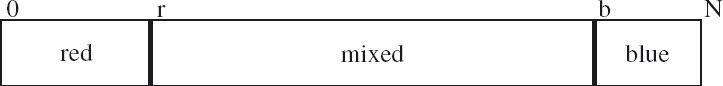
Figure 9.1: The invariant property.

Note that, as required, the precondition is an instance of the invariant shown in Figure 9.1: the precondition is that the entire row of pebbles is mixed and the red and blue segments are empty. The postcondition is also an instance: the postcondition is that the mixed segment is empty. In this way, the invariant generalises from the precondition and postcondition. An obvious measure of progress is the size of the mixed segment. Our goal is to write a loop that maintains the invariant while making progress by always reducing the size of the mixed segment.

Figure 9.1 introduces the variables r and b to represent the extent of the red and blue segments. Expressed formally, the invariant is

0 ≤ r ≤ b ≤ N ∧ ∀i : 0 ≤ i < r : red.i ∧ ∀i : b ≤ i < N : blue.i .

In the initial state, the red and blue segments are empty. We express this by beginning the algorithm with the assignment

r,b := 0,N.

This assignment is said to truthify the invariant. The inequality

0 ≤ r ≤ b ≤ N

is truthified because the size of the row, N, is at least 0 and the two universal quantifications are truthified because 0 ≤ i < 0 and N ≤ i < N are everywhere false.

The size of the mixed segment is b−r; this is our measure of progress. The mixed segment becomes empty by truthifying b−r = 0 , that is, by truthifying r = b; so r = b will be our termination condition.

In order to make progress towards the termination condition, we must increase r and/or decrease b. We can do this by examining the colour of the elements at the boundaries of the ‘mixed’ segment. If the pebble with index r is red, the red segment can be extended by incrementing r. That is, execution of

red.r → r := r+1

is guaranteed to reduce b−r and maintain the invariant. Similarly, if the pebble with index b is blue, the blue segment can be extended by decrementing b. That is, execution of

blue.(b−1) → b := b−1

is guaranteed to reduce b−r and maintain the invariant. Finally, since red.r blue.r and red.(b−1) blue.(b−1), if the pebble with index r is not red and the pebble with index b−1 is not blue, they must be blue and red, respectively; so they can be swapped, and r can be incremented and b can be decremented. That is, execution of

blue.r ∧ red.(b−1) → swap(r , b−1) ; r,b := r+1 , b−1

is guaranteed to reduce b−r and maintain the invariant. The complete solution is shown in Figure 9.2.

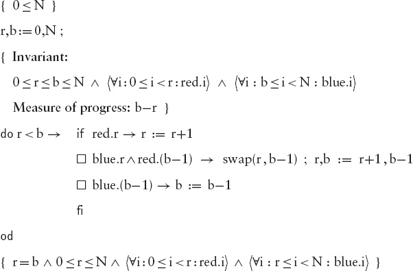
Figure 9.2: A simple sorting algorithm.

Take care to study this algorithm carefully. It exemplifies how to document loops. The boolean expressions in curly brackets are called assertions; they document properties of the state during the execution of the algorithm. The first and last lines document the precondition and postcondition; the precondition is assumed, the postcondition is the goal. The invariant states precisely the function of the variables r and b, and the measure of progress indicates why the loop is guaranteed to terminate. Note that the postcondition is the conjunction of the invariant and the termination condition. Make sure that you understand why the invariant is maintained by the loop body, and why b−r functions as a measure of progress. (We have omitted some essential details in our informal justification of the algorithm. Can you explain, for example, why r ≤ b is maintained by the loop body, and why that is important?)

9.3 BINARY SEARCH

The so-called intermediate-value theorem in mathematics states that if a continuous function is negative at one end of a (non-empty) interval and positive at the other end, it must equal 0 at some ‘intermediate’ point in the interval. The theorem is illustrated in Figure 9.3. The left figure shows the graph of a continuous function in a certain interval; the function’s value is 0 where it crosses the horizontal line. At the left end of the interval the function’s value is negative and at the right end it is positive. In this case there happens to be three points, indicated in the figure by short vertical lines, at which the function’s value is 0; the theorem states that there must be at least one such point.

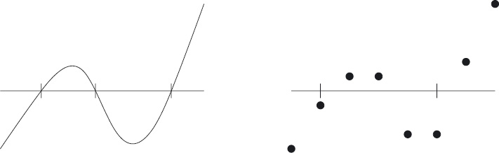
Figure 9.3: The intermediate-value theorem and its discrete counterpart.

The right part of Figure 9.3 illustrates the discrete analogue of the intermediate-value theorem. Suppose a function f is defined on some non-empty interval of the natural numbers and suppose at the left end of the interval the function’s value is at most 0 and at the right end the function’s value is at least 0. Then there must be a point i in the interval such that f(i) ≤ 0 ≤ f(i+1). (In our example, there are two possible values for i indicated by short vertical lines.) In this section, we show how to search for such a point in a very efficient way. The method is called binary search.

We assume that the interval is given by two (natural) numbers M and N. The precondition is that the interval is non-empty, i.e. M<N, and the function f has opposite sign at the two ends of the interval, i.e. f(M) ≤ 0 ≤ f(N). The goal is to determine a number i such that f(i) ≤ 0 ≤ f(i+1).

Comparing the precondition

M<N ∧ f(M) ≤ 0 ≤ f(N)

with the postcondition

f(i) ≤ 0 ≤ f(i+1),

it is obvious that both are instances of

where i and j are variables. This suggests that our algorithm should introduce two variables i and j which are initialised to M and N, respectively; the algorithm will then be a loop that maintains (9.1) whilst making progress to the condition that i+1 = j. An obvious measure of progress is the size of the interval j−i.

Formally, this is the structure of the algorithm so far:

{ M<N ∧ f(M) ≤ 0 ≤ f(N) }

i,j := M,N

{ Invariant: i<j ∧ f(i) ≤ 0 ≤ f(j)

   Measure of progress: j−i };

do i+1 ≠ j → body

od

{ i+1 = j ∧ f(i) ≤ 0 ≤ f(i+1) }

The initial assignment truthifies the invariant. Assuming that the loop body maintains the invariant, when the loop terminates we have:

i+1 = j ∧ i<j ∧ f(i) ≤ 0 ≤ f(j)

which simplifies to

i+1 = j ∧ f(i) ≤ 0 ≤ f(i+1).

The value of i thus satisfies the goal.

Now we have to construct the loop body. We make progress by reducing the size of the interval, which is given by j−i. Reducing j−i is achieved either by reducing j or by increasing i. Clearly, in order to simultaneously maintain the invariant, it is necessary to examine the value of f(k) for at least one number k in the interval. Suppose we choose an arbitrary k such that i<k<j and inspect f(k). Then either f(k) ≤ 0 or 0 ≤ f(k) (or both, but that is not important). In the former case, the value of i can be increased to k and, in the latter case, the value of j can be decreased to k. In this way, we arrive at a loop body of the form:

{ i+1 ≠ j ∧ i<j ∧ f(i) ≤ 0 ≤ f(j) }

choose k such that i<k<j

{ i<k<j ∧ f(i) ≤ 0 ≤ f(j) };

if f(k) ≤ 0 → i := k

□ 0 ≤ f(k) → j := k

fi

{ i<j ∧ f(i) ≤ 0 ≤ f(j) }

Note that i+1 ≠ j ∧ i<j simplifies to i+1 < j or equally i < j−1 so that it is always possible to choose k: two possible choices are i+1 and j−1. The final step is to decide how to choose k.

Always choosing i+1 for the value of k gives a so-called linear search whereby the value of j is constant and i is incremented by 1 at each iteration. (For those familiar with a conventional programming language, such a search would be implemented by a so-called for loop.) Symmetrically, always choosing j−1 for the value of k also gives a linear search whereby the value of i is constant and j is decremented by 1 at each iteration. In both cases, the size of the interval is reduced by exactly one at each iteration --- which isn’t very efficient. Binary search is somewhat better. By choosing a value k roughly half-way between i and j, it is possible to reduce the size of the interval by roughly a half at each iteration. This choice is implemented by the assignment:

k := (i+j)÷2.

Substituting these design decisions in the algorithm above, we get the complete algorithm:

{ M<N ∧ f(M) ≤ 0 ≤ f(N) }

i,j := M,N

{ Invariant: i<j ∧ f(i) ≤ 0 ≤ f(j)

   Measure of progress: j−i };

do i+1 ≠ j →    { i+1 = j ∧ i<j ∧ f(i) ≤ 0 ≤ f(j) }

                        k := (i+j)÷2

                       { i<k<j ∧ f(i) ≤ 0 ≤ f(j) };

                       if  f(k) ≤ 0 →   i := k

                       □ 0 ≤ f(k)  →   j := k

                       fi

                       { i < j ∧ f(i) ≤ 0 ≤ f(j) }

od

{ i+1 = j ∧ f(i) ≤ 0 ≤ f(i+1) }

The correctness of the algorithm relies on the property that

[ i+1 ≠ j ∧ i<j    ⇒    i < (i+j)÷2 < j  ] .

This property can be proven using the properties of integer division discussed in section 15.4.1. The measure of progress, the size of the interval, only gives an upper bound on the number of iterations of the loop body. In this algorithm, because j−i is halved at each iteration, the number of iterations is approximately log₂(N−M). So, for example, if N−M is 1024 (i.e. 2¹⁰), the number of iterations is 10. This is independent of the function f. The number of iterations required by a linear search is at least 1 and at most 1023, depending on the function f. So linear search is much worse in the worst case (although it is not always worse).

9.4 SAM LOYD’S CHICKEN - CHASING PROBLEM

For our next example of algorithm design, we construct an algorithm to solve a puzzle invented by Sam Loyd. Here is Loyd’s (slightly modified) description of the problem:²

On a New Jersey farm, where some city folks were wont to summer, chicken-chasing became an everyday sport, and there were two chickens which could always be found in the garden ready to challenge any one to catch them. It reminded one of a game of tag, and suggests a curious puzzle which I am satisfied will worry some of our experts.

The object is to prove in just how many moves the good farmer and his wife can catch the two chickens.

The field is divided into sixty-four square patches, marked off by the corn hills. Let us suppose that they are playing a game, moving between the corn rows from one square to another, directly up and down or right and left.

Play turn about. First let the man and woman each move one square, then let each of the chickens make a move. The play continues in turns until you find out in how many moves

it is possible to drive the chickens into such positions that both of them are cornered and captured. A capture occurs when the farmer or his wife can pounce on a square occupied by a chicken.

The game can be played on any checkerboard by using two checkers of one color to represent the farmer and his wife, and two checkers of another color to represent the hen and rooster.

The game is easy to solve; the only trick in the problem is that, in the initial state depicted in Loyd’s accompanying illustration (see Figure 9.4), the farmer cannot catch the rooster and his wife cannot catch the hen. This is obvious to anyone trained to look out for invariants. The farmer is given the first move and his distance from the rooster (measured by smallest number of moves needed to reach the rooster) is initially even. When the farmer moves the distance becomes odd. The rooster’s next move then makes the distance even again. And so it goes on. The farmer can thus never make the distance zero, which is an even number. The same argument applies to his wife and the hen. However, the farmer is initially at an odd distance from the hen and his wife is an odd distance from the rooster, so the problem has to be solved by the farmer chasing the hen and his wife chasing the rooster. This argument is even more obvious when the game is played on a chessboard. Squares on a chessboard that have the same colour are an even distance apart (where distance is measured as the smallest number of horizontal and/or vertical moves needed to move from one square to the other) and squares that have different colours are an odd distance apart. Any single horizontal or vertical move is between squares of different colour.

Figure 9.4: The chicken-chasing problem.

As we said, the game is easy to solve. Try it and see. (It is possible to play the game on the Internet. See the bibliographic remarks in Section 9.7.) The real challenge is to articulate the solution to the problem sufficiently precisely that it can be executed by a dumb machine. This is what this section is about.

In some respects, Loyd’s formulation of the problem is unclear. He does not say whether or not the farmer and his wife can occupy the same square on the board and he does not say what happens if the hen or rooster moves to a square occupied by the farmer or his wife. Partly to avoid the distractions of such details, we consider a simplified form of the game.

The problem we consider assumes a rectangular checkerboard of arbitrary, but finite, dimension. There are just two players, the hunter and the prey. The hunter occupies one square of the board and the prey occupies another square. The hunter and prey take it in turns to move; a single move is one square vertically or horizontally (up or down or to the right or left) within the bounds of the board (see Figure 9.5). The hunter catches the prey if the hunter moves to the square occupied by the prey. The problem is to formulate an algorithm that guarantees that the hunter catches the prey with the smallest number of moves.

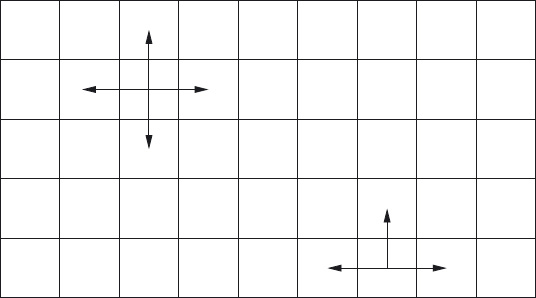
Figure 9.5: Allowed moves in the catching game.

Our solution is to first formulate an algorithm that guarantees the capture of the prey. Then we will argue that the algorithm achieves its task in the smallest possible number of moves.

The distance between the prey and the hunter clearly plays a fundamental role in the algorithm, so we begin by formulating the notion precisely.

Given any two squares on the board we can identify the horizontal distance, h, and the vertical distance, v, between them, as shown in Figure 9.6. (To be completely precise, if each square is assigned cartesian coordinates, the horizontal distance between square (i, j) and square (k, l) is |i−k| and the vertical distance between them is |j−l|.) The (total) distance, d, between the two squares is h+v. (This is sometimes called the Manhattan distance after the layout of streets in Manhattan, New York.)

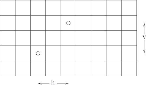
Figure 9.6: Horizontal and vertical distances.

If the prey and hunter are initially distance d apart and one of them makes a single move, d is either incremented or decremented by one. If they each take a turn to move, the effect is to execute the sequence of assignments

d := d ± 1 ; d := d ± 1.

This is equivalent to executing

d := d−2  □  d := d+0  □  d := d+2.

(Recall that “ □ ” denotes a non-deterministic choice – see Section 2.3.1.) An obvious invariant is the boolean quantity even(d). (If d is even, i.e. even(d) has the value true, it will remain even and if d is odd, i.e. even(d) has the value false, it will remain odd.) Since the goal is to reduce the distance to 0, which is even, it is necessary to assume that the prey and hunter are an odd distance apart when the hunter makes its first move. This assumption becomes a precondition of our algorithm.

Loyd’s statement of the problem suggests the obvious strategy: the goal is to corner the prey. But what is meant precisely by “corner”? We let the mathematics be our guide.

Let h and v denote, respectively, the (absolute) horizontal and vertical distances between the hunter and the prey. Let us suppose the hunter is allowed the first move. Then the problem is to formulate an algorithm S satisfying

{ odd(h+v) }

S

{ h = 0 = v }.

The form of S must reflect the fact that the moves of the prey and the hunter alternate, with the prey’s moves being expressed as non-deterministic choices. In contrast, the hunter’s moves must be fully determined. The precondition odd(h+v) is essential in the case where the hunter makes the first move, as argued above. The postcondition expresses formally the requirement that, on termination of S, the distance between the prey and hunter is zero. Furthermore, it is important to note that h and v are natural numbers and not arbitrary integers (since they record absolute distances). For the moment, we say nothing about the size of the board, although this is clearly an essential component of any solution.

The postcondition suggests a possible sequential decomposition of the problem: first the hunter “corners” the prey by truthifying h = v and then, assuming h = v, the hunter catches the prey.

{  odd(h+v)  }

get the prey into a corner

{  h = v  };

catch the prey

{  h = 0 = v  }.

Diagrammatically one can understand why truthifying h = v is expressed in words as “cornering” the prey. In such a state, the hunter and prey are connected by a diagonal line which identifies a unique corner of the board: each diagonal identifies two corners and, of these, the one closest to the prey is chosen. For example, in the state shown in Figure 9.7, the hunter’s task is to drive the prey into the bottom-left corner of the board.

9.4.1 Cornering the Prey

We begin with the task of truthifying h = v. Initially, h = v is false (because h+v is odd). That is, h < v ∨ v < h. Now note that what we call “horizontal” and what we call “vertical” is somewhat arbitrary since rotating the board through 90^° interchanges the two. So, by rotating the board if necessary, we may assume that h < v. Then all the hunter has to do is to repeatedly move vertically, in the direction towards the prey thus decreasing v, until h = v is true, irrespective of the prey’s moves.

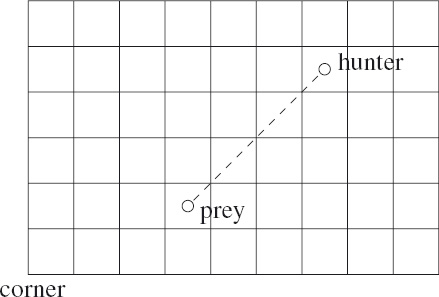
Figure 9.7: The prey is cornered.

Is this really correct? Are we not forgetting that the prey moves too? Let us put it to the test. Below we give a skeleton of the algorithm showing just the hunter’s moves. The precondition is odd(h+v) ∧ h < v and the postcondition is h = v. The hunter’s moves are modelled by the assignments v := v−1. The hunter makes its first move and then the prey and hunter alternate in making a move. The loop is terminated if h and v are equal (this is the function of the guard h ≠ v).

{ odd(h+v) ∧ h < v }

v := v−1 ;

do h ≠ v →   prey’s move ;

                      v := v−1

od

{ h = v }

Now we add to this skeleton an if–fi statement that reflects a superset of the options open to the prey. (We explain later why it is a superset.) In addition, we document the loop with an all-important invariant property and measure of progress. These are the key to the correctness of this stage of the algorithm. Several assertions have also been added in the body of the loop; the one labelled PreP is the precondition for the prey’s move. The variable vp has also been introduced; this is the vertical distance of the prey from the “bottom” of the board. Very importantly, we define the bottom of the board so that the prey is below the hunter on the board, that is, the bottom is the side of the board such that the vertical distance of the prey from the bottom is smaller than the vertical distance of the hunter from the bottom. (If necessary, the board can always be rotated through 180^◦ so that what we normally understand by “bottom” and “below” fits with the definition.) The reason why this is important becomes clear when we discuss the termination of the loop.

{ odd(h+v) ∧ h < v }

/∗ hunter’s move ∗/

v := v−1

{ Invariant: even(h+v) ∧ h ≤ v

   Measure of progress: v+vp } ;

do h ≠ v→   /∗   prey’s move ∗/

                  { PreP: even(h+v) ∧ h+1 < v }

                  if h ≠ 0 → h := h−1

                  □ true → h := h+1

                  □ vp ≠ 0 → v , vp := v+1 , vp−1

                  □ true → v , vp := v−1 , vp+1

                  fi

                  { odd(h+v) ∧ h < v } ;

                  /∗ hunter’s move ∗/

                  v := v−1

                  { even(h+v) ∧ h ≤ v }

od

{ h = v }

The precondition of the hunter’s first move is

odd(h+v) ∧ h < v.

We see shortly that this is a precondition of all of the hunter’s moves in this cornering phase of the algorithm. From such a state, the hunter’s move truthifies the property

even(h+v) ∧ h ≤ v.

This is the invariant of the loop.

Now, either h=v or h<v. In the former case, the loop terminates and the desired postcondition has been truthified. In the latter case, the conjunction of h<v and the invariant becomes the precondition, PreP, of the prey’s move. But

even(h+v) ∧ h ≤ v ∧ h < v even(h+v) ∧ h+1 < v

so the prey chooses a move with precondition

even(h+v) ∧ h+1 < v.

This assertion is labelled PreP above. Now we show that with precondition PreP, a move by the prey truthifies the condition

which, we recall, was the precondition of the hunter’s first move.

The prey can choose between four options: increase/decrease the horizontal/vertical distance from it to the hunter. These are the four branches of the if–if statement. The guard “h ≠ 0” has been added to the option of decreasing the horizontal distance; if h is 0, a horizontal move by the prey will increase its horizontal distance from the hunter. The guard on the action of increasing v and decreasing vp is necessary for our argument; it constrains the movements of the prey in a vertical direction. The guards on horizontal movements could be strengthened in a similar way; we have not done so because constraints on the prey’s horizontal movements are not relevant at this stage. Indeed, the hunter’s algorithm has to take account of all possible moves the prey is allowed to make; if the algorithm takes account of a superset of such possibilities, the correctness is still assured.

Because the hunter has no control over the prey’s choice of move, we have to show that (9.2) is truthified irrespective of the choice. It is obvious that all four choices falsify even(h+v) and truthify odd(h+v) (because exactly one of h and v is incremented or decremented by 1). Also, all four choices truthify h < v. In the two cases where the prey’s move increases h or decreases v, we need to exploit the fact that h+1 < v before the move. The other two cases are simpler. The guard on increasing the vertical distance is not needed at this stage in the argument.

We have shown that, if the loop begins in a state that satisfies the invariant, re-execution of the loop will also begin in a state that satisfies the invariant. The question that remains is whether or not the loop is guaranteed to terminate. Do we indeed make progress to the state where h and v are equal?

It is at this point that the variable vp is needed. Recall that vp is the distance of the prey from the bottom of the board. Recall also that the definition of ‘bottom’ is such that the prey is closer to the bottom than the hunter. This means that v+vp is the distance of the hunter from the bottom of the board.

The crucial fact is that, when the prey increases v, the value of vp decreases by the same amount; conversely, when the prey decreases v, the value of vp increases by the same amount. Thus v+vp is an invariant of the prey’s move. However, since the hunter’s move decreases v, the net effect of a move by the hunter followed by the prey is to decrease v+vp by 1; but its value is always at least zero. So the repetition of such a pair of moves can only occur a finite number of times (in fact, at most the initial vertical distance of the hunter from the bottom of the board). The loop is guaranteed to terminate in a state where h and v are equal and the prey is cornered.

9.4.2 Catching the Prey

Unlike the cornering process, catching the prey requires the hunter to adapt its moves according to the moves made by the prey.

The precondition for this stage is h = v. Recall that this condition identifies a unique corner of the board, which we call “the” corner. If hp is the horizontal distance of the prey from the corner, the horizontal distance of the hunter from the corner is h+hp. Similarly, if vp is the vertical distance of the prey from the corner, the vertical distance of the hunter from the corner is v+vp.

Starting in a state that satisfies h = v, any move made by the prey will falsify the property; the hunter’s response is to truthify the property while making progress to the termination condition h = 0.

It is easy to truthify h = v following a move by the prey. Figure 9.8 shows two ways this can be done when the prey moves in a way that increases h; the hunter may respond by moving horizontally or vertically. Although the vertical move may not be possible because of the boundary of the board, the horizontal move is always possible. Moreover, the horizontal move makes progress in the sense that the hunter moves closer to the corner.

The full details of how the hunter should respond to a move by the prey are shown below. The tests hp ≠ 0 and vp ≠ 0 prevent the prey from moving off the board in the direction away from the hunter. The distance of the hunter from the corner is h+hp+v+vp. This is the bound on the number of times the loop body is executed.

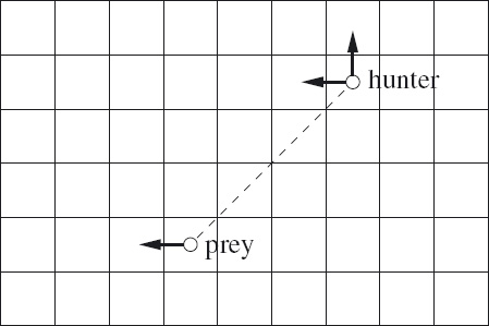
Figure 9.8: Maintaining the catching invariant.

{ Invariant: h = v

   Measure of progress:     h+hp+v+vp }

do 0 < h →   if   hp = 0 →   /∗   prey’s move  ∗/

                                              hp , h := hp−1 , h+1 ;

                                             /∗ hunter’s move ∗/

                                             h := h−1

                    □  true  →      /∗   prey’s move ∗/

                                         hp , h := hp+1 , h−1 ;

                                        /∗     hunter’s move ∗/

                                        v := v−1

                    □  vp ≠ 0 →   /∗ prey’s move  ∗/

                                         vp , v := vp−1 , v+1 ;

                                         /∗    hunter’s move ∗/

                                         v := v−1

                   □  true   →  /∗   prey’s move  ∗/

                                        vp , v := vp+1 , v−1 ;

                                        /∗ hunter’s move  ∗/

                                        h := h−1

                  fi

od

{ h = 0 = v }

It is easy to check that the net effect of a move by the prey followed by a move by the hunter is to truthify h = v. Progress is made to the termination condition because both h+hp and v+vp are invariants of the prey’s moves while the hunter’s move always decreases either h or v. The distance h+hp+v+vp is thus always decreased but cannot be decreased forever because it is always at least zero. This completes the algorithm.

9.4.3 Optimality

We conclude the discussion by considering whether the algorithm is optimal. For brevity, the argument is informal, although it can be made formal. Once again, the notion of an invariant plays an important role.

We have established that the hunter can always catch the prey (assuming the two are initially at an odd distance apart) by presenting an algorithm whereby the hunter chooses its moves. To establish the optimality of the hunter’s algorithm, we have to switch the focus to the prey. Although the prey cannot avoid capture, it can try to evade the hunter for as long as possible. We must investigate the prey’s algorithm to do this.

The hunter’s algorithm has two phases. In the cornering phase, the hunter continually moves in one direction, vertically downwards. In the catching phase, the hunter moves steadily towards “the” corner, either horizontally or vertically. The total distance moved by the hunter is thus at most its initial distance from the corner to which the prey is driven.

The corner to which the prey is driven is not chosen by the hunter; it is determined by the prey’s moves in the cornering phase. A choice of two possible corners is made, however, prior to the cornering phase. (It is this choice that allows us to assume that h < v initially.) Let us call these two corners A and B, and the remaining two corners C and D. Initially, the prey is closer than the hunter to A and to B; conversely, the hunter is closer than the prey to C and to D.

The hunter cannot catch the prey in corners C or D because, after each of the hunter’s moves, the prey can always truthify the property that the hunter is closer than the prey to C and to D. The hunter must therefore catch the prey in corner A or B.

Now suppose corner A is strictly closer to the hunter than corner B. (If the two corners are at equal distance from the hunter, it does not matter which of the two the prey is caught in.) Now the prey can always force the hunter to move a distance at least equal to the hunter’s initial distance from corner B. One way the prey can do this is to continually choose the option of reducing its horizontal distance, h, from the hunter during the cornering phase; when forced to increase h – when h=0 – the prey moves towards corner B. This guarantees making progress to the postcondition h=v=1 while maintaining the property that the prey is closer to corner B than the hunter. In the catching phase, the prey continually chooses between increasing h and increasing v while it still can. (It cannot do so indefinitely because of the boundaries of the checkerboard.) The invariant in this phase is that either 0<h or 0<v or the prey is at corner B. When the prey is at corner B, it will be caught after its next move.

In this way it is proven that the hunter moves a distance that is at least its initial distance from corner B. Since we have already shown that the hunter moves a distance that is at most its initial distance from corner B, we have established that the hunter’s algorithm is optimal.

9.5 PROJECTS

The following are exercises in algorithm design similar to the chicken-chasing problem. They are non-trivial, which is why we have titled the section ‘Projects’. Do not expect to solve them in a short time: algorithm design demands careful work in order to get it right. The solution to the first exercise is provided at the end of the book, the second is not.

9.7 BIBLIOGRAPHIC REMARKS

Section 9.2 is a simplification of a sorting problem (involving three colours) called the Dutch national flag problem, introduced by E.W. Dijkstra. Dijkstra’s original description of the Dutch national flag problem can be found in his classic text, A Discipline of Programming [Dij76]. There, you will also find many other examples of derivations of non-trivial algorithms. The Dutch national flag problem is a subroutine in a general-purpose sorting algorithm called Quicksort and a program called Find for finding the k smallest elements in an array, both of which were designed by C.A.R. Hoare. These algorithms are discussed in many texts on algorithm design.

Binary search is often used as an introductory example of algorithm design, but most texts – including one written by myself – assume a much stronger precondition. (It is common to assume that the function f is monotonic.) The fact that the precondition can be significantly weakened, as here, is not well known; it is due to David Gries [Gri81].

The chicken-chasing problem was invented by Sam Loyd (Cyclopedia of Puzzles, Lamb Publishing, New York, 1914). It is one of many mathematical puzzles listed at http://www.cut-the-knot.org; the website has an applet so that you can play the game. The algorithm presented here is based on a derivation by Diethard Michaelis.

The Chameleons of Camelot problem (Exercise 9.5) is a generalisation of a problem found in [Hon97, page 140]. The problem was formulated and solved by João F. Ferreira [Fer10].

Exercise 9.4 was posed to me by Dmitri Chubarov. I have been told that it was posed in a slightly different form in the Russian national Mathematics Olympiad in 1975 and appears in a book by Vasiliev entitled Zadachi Vsesoyuzynykh Matematicheskikh Olympiad, published in Moscow in 1988. The author of the problem is apparently not stated.

¹ Strictly, a loop invariant is not an invariant but what is sometimes called a mono-invariant. A mono-invariant is a value in an ordered set that always changes monotonically, that is, either remains constant or increases at each step. A loop invariant is a boolean function of the state that either remains constant or increases with respect to the implication ordering on booleans. This means that, if the value of the loop invariant is false before execution of the loop body, its value may change to true.

² See http://www.cut-the-knot.org/SimpleGames/RFWH.shtml.