Table of Contents for
Algorithmic Problem Solving
 Algorithmic Problem Solving
Published by
John Wiley & Sons, 2011
Algorithmic Problem Solving
Published by
John Wiley & Sons, 2011
- Coverpage
- Algorithmic Problem Solving
- Titlepage
- Copyright
- Preface
- Contents
- PART I: Algorithmic Problem Solving
- CHAPTER 1: Introduction
- CHAPTER 2: Invariants
- CHAPTER 3: Crossing a River
- CHAPTER 4: Games
- CHAPTER 5: Knights and Knaves
- CHAPTER 6: Induction
- CHAPTER 7: Fake-Coin Detection
- CHAPTER 8: The Tower of Hanoi
- CHAPTER 9: Principles of Algorithm Design
- CHAPTER 10: The Bridge Problem
- CHAPTER 11: Knight’s Circuit
- PART II: Mathematical Techniques
- CHAPTER 12: The Language of Mathematics
- CHAPTER 13: Boolean Algebra
- CHAPTER 14: Quantifiers
- CHAPTER 15: Elements of Number Theory
- CHAPTER 16: Relations, Graphs and Path Algebras
- Solutions to Exercises
- References
- Index

“Invariant” means “not changing”. An invariant of some process is some attribute or property of the process that does not change. Other names for “invariant” are “constant” and “pattern”.
The recognition of invariants is an important problem-solving skill, possibly the most important. This chapter introduces the notion of an invariant and discusses a number of examples of its use.
We first present a number of problems for you to tackle. Some you may find easy, but others you may find difficult or even impossible to solve. If you cannot solve one, move on to the next. To gain full benefit, however, it is better that you try the problems first before reading further.
We then return to each of the problems individually. The first problem we discuss in detail, showing how an invariant is used to solve the problem. Along the way, we introduce some basic skills related to computer programming – the use of assignment statements and how to reason about assignments. The problem is followed by an exercise which can be solved using very similar techniques.
The second problem develops the techniques further. It is followed by a discussion of good and bad problem-solving techniques. The third problem is quite easy, but it involves a new concept, which we discuss in detail. Then, it is your turn again. From a proper understanding of the solution to these initial problems, you should be able to solve the next couple of problems. This process is repeated as the problems get harder; we demonstrate how to solve one problem, and then leave you to solve some more. You should find them much easier to solve.
1. Chocolate Bars A rectangular chocolate bar is divided into squares by horizontal and vertical grooves, in the usual way. It is to be cut into individual squares. A cut is made by choosing a piece and cutting along one of its grooves. (Thus each cut splits one piece into two pieces.)
Figure 2.1 shows a 4×3 chocolate bar that has been cut into five pieces. The cuts are indicated by solid lines.

 Figure 2.1: Chocolate-bar problem.
How many cuts are needed to completely cut the chocolate into all its squares?
2. Empty Boxes Eleven large empty boxes are placed on a table. An unknown number of the boxes is selected and, into each one, eight medium boxes are placed. An unknown number of the medium boxes is selected and, into each one, eight small boxes are placed.
At the end of this process there are 102 empty boxes. How many boxes are there in total?
3. Tumblers Several tumblers are placed on a table. Some tumblers are upside down, some are upside up. (See Figure 2.2.) It is required to turn all the tumblers upside up. However, the tumblers may not be turned individually; an allowed move is to turn any two tumblers simultaneously.

From which initial states of the tumblers is it possible to turn all the tumblers upside up?
4. Black and White Balls Consider an urn filled with a number of balls each of which is either black or white. There are also enough balls outside the urn to play the following game. We want to reduce the number of balls in the urn to one by repeating the following process as often as necessary.
Take any two balls out of the urn. If both have the same colour, throw them away but put another black ball into the urn; if they have different colours, return the white one to the urn and throw the black one away.
Each execution of the above process reduces the number of balls in the urn by one; when only one ball is left the game is over.
What, if anything, can be said about the colour of the final ball in the urn in relation to the original number of black balls and white balls?
5. Dominoes A chessboard has had its top-right and bottom-left squares removed so that 62 squares remain (see Figure 2.3). An unlimited supply of dominoes has been provided; each domino will cover exactly two squares of the chessboard.
Is it possible to cover all 62 squares of the chessboard with the dominoes without any domino overlapping another domino or sticking out beyond the edges of the board?

Figure 2.3: Mutilated chess board.
6. Tetrominoes A tetromino is a figure made from 4 squares of the same size. There are five different tetrominoes, called the O-, Z-, L-, T- and I-tetrominoes. (See Figure 2.4.)
The following exercises concern covering a rectangular board with tetrominoes. Assume that the board is made up of squares of the same size as the ones used to make the tetrominoes. Overlapping tetrominoes or tetrominoes that stick out from the sides of the board are not allowed.
(a) Suppose a rectangular board is covered with tetrominoes. Show that at least one side of the rectangle has an even number of squares.
(b) Suppose a rectangular board can be covered with T-tetrominoes. Show that the number of squares is a multiple of 8.
(c) Suppose a rectangular board can be covered with L-tetrominoes. Show that the number of squares is a multiple of 8.
(d) An 8×8 board cannot be covered with one O-tetromino and fifteen L-tetrominoes. Why not?
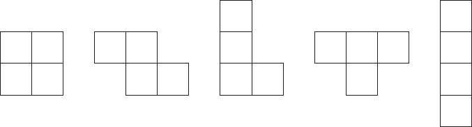
Figure 2.4: O-, Z-, L-, T- and I-tetromino.
Note that all of these problems involve an algorithm. In each case, the algorithm involves repeating a simple process (cutting the chocolate bar, filling a box, turning two tumblers, etc.). This is not difficult to spot. Whenever an algorithm has this form, the first task is to identify the “invariants” of the algorithm. This important skill is the focus of this chapter.
2.1 CHOCOLATE BARS
Recall the problem statement:
A rectangular chocolate bar is divided into squares by horizontal and vertical grooves, in the usual way. It is to be cut into individual squares. A cut is made by choosing a piece and cutting along one of its grooves. (Thus each cut splits one piece into two pieces.)
How many cuts are needed to completely cut the chocolate into all its squares?
2.1.1 The Solution
Here is a solution to the chocolate-bar problem. Whenever a cut is made, the number of cuts increases by one and the number of pieces increases by one. Thus, the number of cuts and the number of pieces both change. What does not change, however, is the difference between the number of cuts and the number of pieces. This is an “invariant”, or a “constant”, of the process of cutting the chocolate bar.
We begin with one piece and zero cuts. So, the difference between the number of pieces and the number of cuts, at the outset, is one. It being a constant means that it will always be one, no matter how many cuts have been made. That is, the number of pieces will always be one more than the number of cuts. Equivalently, the number of cuts will always be one less than the number of pieces.
We conclude that to cut the chocolate bar into all its individual squares, the number of cuts needed is one less than the number of squares.
2.1.2 The Mathematical Solution
Once the skill of identifying invariants has been mastered, this is an easy problem to solve. For this reason, we have used English to describe the solution, rather than formulating the solution in a mathematical notation. For more complex problems, mathematical notation helps considerably, because it is more succinct and more precise. Let us use this problem to illustrate what we mean.
 Throughout the text we use the language of mathematics to make things precise. For example, we use words like “function” and “set” with their mathematical meaning, sometimes without introduction. Part II of this book, on mathematical techniques, provides the necessary background. Chapter 12 introduces much of the vocabulary. Consult this chapter if unfamiliar terms are used.
Abstraction The mathematical solution begins by introducing two variables. We let variable p be the number of pieces and c be the number of cuts. The values of these variables describe the state of the chocolate bar.
This first step is called abstraction. We “abstract” from the problem a collection of variables (or “parameters”) that completely characterise the essential elements of the problem. In this step, inessential details are eliminated.
One of the inessential details is that the problem has anything to do with chocolate bars! This is totally irrelevant and, accordingly, has been eliminated. The problem could equally well have been about cutting postage stamps from a sheet of stamps. The problem has become a “mathematical” problem, because it is about properties of numbers, rather than a “real-world” problem. Real-world problems can be very hard, if not impossible, to solve; in contrast, problems that succumb to mathematical analysis are relatively easy.
Other inessential details that have been eliminated are the sequence of cuts that have been made and the shapes and sizes of the resulting pieces. That is, the variables p and c do not completely characterise the state of the chocolate bar or the sequence of cuts that have been made to reach that state. Knowing that, say, four cuts have been made, making five pieces, does not allow us to reconstruct the sizes of the individual pieces. That is irrelevant to solving the problem.
The abstraction step is often the hardest step to make. It is very easy to fall into the trap of including unnecessary detail, making the problem and its solution over-complicated. Conversely, deciding what is essential is far from easy: there is no algorithm for making such decisions! The best problem-solvers are probably the ones most skilled in abstraction.
(Texts on problem solving often advise drawing a figure. This may help to clarify the problem statement – for example, we included Figure 2.1 in order to clarify what is meant by a cut – but it can also be a handicap! There are two reasons. The first is that extreme cases are often difficult to capture in a figure. This is something we return to later. The second is that figures often contain much unnecessary detail, as exemplified by Figure 2.1. Our advice is to use figures with the utmost caution; mathematical formulae are often far more effective.)
Assignments The next step in the problem’s solution is to model the process of cutting the chocolate bar. We do so by means of the assignment statement
p , c := p+1 , c+1.
An assignment statement has two sides, a left side and a right side. The two sides are separated by the assignment symbol “:=”, pronounced “becomes”. The left side is a comma-separated list of variables (in this case, p , c). No variable may occur more than once on the left side. The right side is a comma-separated list of expressions (in this case, p+1 , c+1). The list must have length equal to the number of variables on the left side.
An assignment effects a change of state. To execute an assignment statement, first evaluate, in the current state, each expression on the right side and then replace the value of each variable on the left side by the value of the corresponding expression on the right side. In our example, the state – the number of pieces and the number of cuts – is changed by evaluating p+1 and c+1 and then replacing the values of p and c by these values, respectively. In words, p “becomes” p + 1, and c “becomes” c+1. This is how the assignment statement models the process of making a single cut of the chocolate bar.
A word of warning (for those who have already learnt to program in a language like Java or C). We use what is called a simultaneous assignment because several variables are allowed on the left side, their values being updated simultaneously once the right side has been evaluated. Most programming languages restrict the left side of an assignment to a single variable. Java is an example. Instead of a simultaneous assignment, one has to write a sequence of assignments. This is a nuisance, but only that. Much worse is that the equality symbol, “=”, is used instead of the assignment symbol, Java again being an example. This is a major problem because it causes confusion between assignments and equalities, which are two quite different things. Most novice programmers frequently confuse the two, and even experienced programmers sometimes do, leading to errors that are difficult to find. If you do write Java or C programs, always remember to pronounce an assignment as “left side becomes right side” and not “left side equals right side”, even if your teachers do not do so. Also, write the assignment with no blank between the left side variable and the “=” symbol, as in p= p+1, so that it does not look symmetric.
An invariant of an assignment is some function of the state whose value remains constant under execution of the assignment. For example, p−c is an invariant of the assignment p , c := p+1 , c+1.
Suppose expression E depends on the values of the state variables. (For example, expression p−c depends on variables p and c.) We can check that E is an invariant simply by checking for equality between the value of E and the value of E after replacing all variables as prescribed by the assignment. For example, the equality
p−c = (p+1) − (c+1)
simplifies to true whatever the values of p and c. This checks that p−c is an invariant of the assignment p , c := p+1 , c+1. The left side of this equality is the expression E and the right side is the expression E after replacing all variables as prescribed by the assignment.
Here is a detailed calculation showing how (p+1) − (c+1) is simplified to p−c. The calculation illustrates the style we will be using throughout the text. The style is discussed in detail in Chapter 12, in particular in Section 12.8. This example provides a simple introduction.
(p+1) − (c+1)
= { [ x−y = x+(−y) ] with x,y := p+1 , c+1 }
(p+1) + (−(c+1))
= { negation distributes through addition }
(p+1) + ((−c)+(−1))
= { addition is associative and symmetric }
p+(−c)+1+(−1)
= { [ x−y = x+(−y) ]
with x,y := p,c and with x,y := 1 , −1,
[ x−x = 0 ] with x := 1 }
p−c.
The calculation consists of four steps. Each step relates two arithmetic expressions. The relation between each expression in this calculation is equality (of numbers). Sometimes other relations occur in calculations (for example, the “at-most” relation).
Each step asserts that the relation holds between the two expressions “everywhere” – that is, for all possible values of the variables in the two expressions. For example, the final step asserts that, no matter what values variables p and c have, the value of the expression p+(−c)+1+(−1) equals the value of expression p−c.
Each step is justified by a hint. Sometimes the hint states one or more laws together with how the law is instantiated. This is the case for the first and last steps. Laws are recognised by the square “everywhere” brackets. For example, “[ x−x = 0 ]” means that x−x is 0 “everywhere”, that is, for all possible values of variable x. Sometimes a law is given in words, as in the two middle steps.
If you are not familiar with the terminology used in a hint – for example, if you do not know what “distributes” means – consult the appropriate section in Part II of the book.
As another example, consider two variables m and n and the assignment
m , n := m+3 , n−1.
We check that m + 3×n is invariant by checking that
m + 3×n = (m+3) + 3×(n−1)
simplifies to true whatever the values of m and n. Simple algebra shows that this is indeed the case. So, increasing m by 3, simultaneously decreasing n by 1, does not change the value of m + 3×n.
Given an expression E and an assignment ls := rs,
E[ls := rs]
is used to denote the expression obtained by replacing all occurrences of the variables in E listed in ls by the corresponding expression in the list of expressions rs. Here are some examples:
(p−c)[p , c := p+1 , c+1] = (p+1) − (c+1),
(m + 3×n)[m , n := m+3 , n−1] = (m+3) + 3×(n−1),
(m+n+p)[m , n , p := 3×n , m+3 , n−1] = (3×n) + (m+3) + (n−1).
The invariant rule for assignments is then the following: E is an invariant of the assignment ls := rs if, for all instances of the variables in E,
E[ls := rs] = E.
The examples we saw above of this rule are, first, p−c is an invariant of the assignment p , c := p + 1 , c + 1 because
(p−c)[p , c := p+1 , c+1] = p−c
for all instances of variables p and c, and, second, m + 3×n is an invariant of the assignment m , n := m+3 , n−1 because
(m + 3×n)[m , n := m+3 , n−1] = m + 3×n
for all instances of variables m and n.
Induction The final step in the solution of the chocolate-bar problem is to exploit the invariance of p−c.
Initially, p = 1 and c = 0. So, initially, p−c = 1. But, p−c is invariant. So, p−c = 1 no matter how many cuts have been made. When the bar has been cut into all its squares, p = s, where s is the number of squares. So, at that time, the number of cuts, c, satisfies s−c = 1. That is, c = s−1. The number of cuts is one less than the number of squares.
An important principle is being used here, called the principle of mathematical induction. The principle is simple. It is that, if the value of an expression is unchanged by some assignment to its variables, the value will be unchanged no matter how many times the assignment is applied. That is, if the assignment is applied zero times, the value of the expression is unchanged (obviously, because applying the assignment zero times means doing nothing). If the assignment is applied once, the value of the expression is unchanged, by assumption. Applying the assignment twice means applying it once and then once again. Both times, the value of the expression remains unchanged, so the end result is also no change. And so on, for three times, four times, etc.
Note that the case of zero times is included here. Do not forget zero! In the case of the chocolate-bar problem, it is vital to solving the problem in the case where the chocolate bar has exactly one square (in which case zero cuts are required).
Summary This completes our discussion of the chocolate-bar problem. A number of important problem-solving principles have been introduced: abstraction, invariants and induction. We will see these principles again and again.
Exercise 2.1 A knockout tournament is a series of games. Two players compete in each game; the loser is knocked out (i.e. does not play any more), the winner carries on. The winner of the tournament is the player that is left after all other players have been knocked out.
Suppose there are 1234 players in a tournament. How many games are played before the tournament winner is decided? (Hint: choose suitable variables, and seek an invariant.)
2.2 EMPTY BOXES
Recall the empty-box problem:
Eleven large empty boxes are placed on a table. An unknown number of the boxes is selected and into each eight medium boxes are placed. An unknown number of the medium boxes is selected and into each eight small boxes are placed.
At the end of this process there are 102 empty boxes. How many boxes are there in total?
This problem is very much like the chocolate-bar problem in Section 2.1 and the knockout-tournament problem in Exercise 2.1. The core of the problem is a simple algorithm that is repeatedly applied to change the state. Given the initial state and some incomplete information about the final state, we are required to completely characterise the final state. The strategy we use to solve the problem is the following.
George Pólya (1887–1985) was an eminent mathematician who wrote prolifically on problem solving. In his classic book How To Solve It, he offered simple but very wise advice on how to approach new problems in mathematics. His step-by-step guide is roughly summarised in the following three steps.
1. Familiarise yourself with the problem. Identify the unknown. Identify what is given.
2. Devise and then execute a plan, checking each step carefully.
3. Review your solution.
Problem solving is, of course, never straightforward. Even so, Pólya’s rough guide is remarkably pertinent to many problems. It is worthwhile thinking consciously about each of the steps each time you encounter a new problem.
1. Identify what is unknown about the final state and what is known.
2. Introduce variables that together represent the state at an arbitrary point in time.
3. Model the process of filling boxes as an assignment to the state variables.
4. Identify an invariant of the assignment.
5. Combine the previous steps to deduce the final state.
The first step is easy. The unknown is the number of boxes in the final state; what is known is the number of empty boxes. This suggests we introduce (in the second step) variables b and e for the number of boxes and the number of empty boxes, respectively, at an arbitrary point in time.
These first two steps are particularly important. Note that they are goal-directed. We are guided by the goal – determine the number of boxes given the number of empty boxes – to the introduction of variables b and e. A common mistake is to try to count the number of medium boxes or the number of small boxes. These are irrelevant, and a solution that introduces variables representing these quantities is over-complicated. This is a key to effective problem solving: keep it simple!
Let us proceed with the final three steps of our solution plan. The problem statement describes a process of filling boxes. When a box is filled, the number of boxes increases by 8; the number of empty boxes increases by 8−1 since 8 empty boxes are added and 1 is filled. We can therefore model the process by the assignment:
b , e := b+8 , e+7.
We now seek to identify an invariant of this assignment.
Until now, the assignments have been simple, and it has not been too hard to identify an invariant. This assignment is more complicated and the inexperienced problem-solver may have difficulty carrying out the task. Traditionally, the advice given might be to guess. But we do not want to rely on guesswork. Another tactic is to introduce a new variable, n say, to count the number of times boxes are filled. For the boxes problem, this is quite a natural thing to do but we reject it here because we want to illustrate a more general methodology by which guesswork can be turned into calculation when seeking invariants. (We return to the tactic of introducing a count in Section 2.2.1.)
We do have to perform some guesswork. Look at the individual assignments to b and to e. The assignment to b is b := b+8. Thus 8 is repeatedly added to b, and b takes on the values b0 (its initial value – which happens to be 11, but that is not important at this stage), b0+8, b0 + 2×8, b0 + 3×8, etc. Similarly, the values of e are e0, e0+7, e0 + 2×7, e0 + 3×7, etc. In mathematical parlance, the successive values of e are called linear combinations of e0 and 7. Similarly, the successive values of b are linear combinations of b0 and 8. The guess we make is that an invariant is some linear combination of b and e. Now we formulate the guess and proceed to calculate.
We guess that, for some numbers M and N, the number M×b + N×e is an invariant of the assignment, and we try to calculate values for M and N as follows:
M×b + N×e is an invariant of b , e := b+8 , e+7
= { definition of invariant }
(M×b + N×e)[b , e := b+8 , e+7] = M×b + N×e
= { definition of substitution }
M×(b+8) + N×(e+7) = M×b + N×e
= { arithmetic }
(M×b + N×e) + (M×8 + N×7) = M×b + N×e
= { cancellation }
M×8 + N×7 = 0
⇐ { arithmetic }
M = 7 ∧ N = −8.
Success! Our calculation has concluded that 7×b − 8×e is an invariant of the assignment. We now have the information we need to solve the boxes problem.
Initially, both of b and e are 11. So the initial value of 7×b − 8×e is −11. This remains constant throughout the process of filling boxes. In the final state we are given that e is 102; so in the final state, the number of boxes, b, is given by the equation
− 11 = 7×b − 8×10².
Solving this equation, we deduce that 115 = b; the number of boxes in the final state is 115.
2.2.1 Review
One of the best ways of learning effective problem solving is to compare different solution methods. This is, perhaps, the only way to identify the “mistakes” that are often made. By “mistakes” we do not mean factual errors, but choices and tracks that make the solution more difficult or impossible to find.
We have already commented that it is a mistake to introduce variables for the number of small boxes, the number of medium boxes and the number of large boxes. Doing so will not necessarily prevent a solution being found, but the solution method becomes more awkward. The mistake is nevertheless commonly made; it can be avoided by adopting a goal-directed approach to problem solving. The first question to ask is: what is the unknown? Then work backwards to determine what information is needed to determine the unknown.
Goal-directed reasoning is evident in our calculation of M and N. The calculation begins with the defining property and ends with values that satisfy that property. The final step is an if step – the linear combination M×b + N×e is an invariant if M is 7 and N is −8. Other values of M and N also give invariants, for example, when M is −7 and N is 8. (The extreme case is when both M and N are 0. In this case, we deduce that 0 is an invariant of the assignment. But the constant 0 is an invariant of all assignments, so that observation does not help to solve the problem!)
The use of if steps in calculations is a relatively recent innovation, and almost unknown in traditional mathematical texts. Mathematicians will typically postulate the solution and then verify that it is correct. This is shorter but hides the discovery process. We occasionally do the same but only when the techniques for constructing the solution are already clear.
The calculation of M and N is another example of the style of calculation we use in this text. The calculation consists of five steps. Each step relates two boolean expressions. For example, the third step relates the expressions

M×(b+8) + N×(e+7) = M×b + N×e (2.2)
(M×b + N×e) + (M×8 + N×7) = M×b + N×e. (2.3)
In all but the last step, the relation is (boolean) equality. In the last step, the relation is “⇐” (pronounced “if”). A boolean expression may evaluate to true or to false depending on the values of the variables in the expression. For example, if the values of M and N are both zero, the value of the expression M×8 + N×7 = 0 is true while the value of M = 7 ∧ N = −8 is false. The symbol “∧” is pronounced “and”.
Each step asserts that the relation holds between the two expressions “everywhere” – that is, for all possible values of the variables in the two expressions. For example, the third step asserts that no matter what value variables M, N, b and e have, the value of the expression (2.2) equals the value of expression (2.3). (For example, if the variables M, N, b and e all have the value 0, the values of (2.2) and (2.3) are both true; if all the variables have the value 1 the values of (2.2) and (2.3) are both false.) The assertion is justified by a hint, enclosed in curly brackets.
The calculation uses three boolean operators – “=”, “⇐” and “∧”. See Section 12.6 for how to evaluate expressions involving these operators. The final step in the calculation is an if step and not an equality step because it is the case that whenever M=7 ∧ N=−8 evaluates to true then so too does M×8 + N×7 = 0. However, when M and N are both 0, the former expression evaluates to false while the latter evaluates to true. The expressions are thus not equal everywhere.
Note that we use the equality symbol “=” both for equality of boolean values (as in the first four steps) and for equality of numbers (as in “M = 7”). This so-called “overloading” of the operator is discussed in Chapter 12.
Another solution method for this problem is to introduce a variable, n say, for the number of times eight boxes are filled. The number of boxes and the number of empty boxes at time n are then denoted using a subscript – b0, b1, b2, etc. and e0, e1, e2, etc. Instead of an assignment, we then have equalities:
bn+1 = bn+8 ∧ en+1 = en+7.
This solution method works for this problem but at the expense of the increased complexity of subscripted variables. We can avoid the complexity if we accept that change of state caused by an assignment is an inescapable feature of algorithmic problem solving; we must therefore learn how to reason about assignments directly rather than work around them.
Such a solution is one that is intermediate between our solution and the solution with subscripted variables: a count is introduced but the variables are not subscripted. The problem then becomes to identify invariants of the assignment
b , e , n := b+8 , e+7 , n+1.
The variable n, which counts the number of times the assignment is executed, is called an auxiliary variable; its role is to assist in the reasoning. Auxiliary variables are, indeed, sometimes useful for more complex problems. In this case, it is perhaps easier to spot that b − 8×n and e − 7×n are both invariants of the assignment. Moroever, if E and F are both invariants of the assignment, any combination E⊕F will also be invariant. So 7×(b − 8×n) − 8×(e − 7×n) is also invariant, and this expression simplifies to 7×b − 8×e. When an assignment involves three or more variables, it can be a useful strategy to seek invariant combinations of subsets of the variables and then combine the invariants into one.
A third way of utilising an auxiliary variable is to consider the effect of executing the assignment
b , e := b+8 , e+7
n times in succession. This is equivalent to one execution of the assignment
b , e := b + n×8 , e + n×7.
Starting from a state where e has the value 11 and ending in a state where e is 102 is only possible if n = 13. The final value of b must then be 11 + 13×8. This solution appears to avoid the use of invariants altogether, but that is not the case: a fuller argument would use invariants to justify the initial claim about n executions of the assignment.
Exercise 2.4 Can you generalise the boxes problem? Suppose there are initially m boxes and then repeatedly k smaller boxes are inserted into one empty box. Suppose there are ultimately n empty boxes. You are asked to calculate the number of boxes when this process is complete. Determine a condition on m, k and n that guarantees that the problem is well-formulated and give the solution.
You should find that the problem is not well formulated when k equals 1. Explain in words why this is the case.
2.3 THE TUMBLER PROBLEM
Recall the statement of the tumbler problem.
Several tumblers are placed on a table. Some tumblers are upside down, some are upside up. It is required to turn all the tumblers upside up. However, the tumblers may not be turned individually; an allowed move is to turn any two tumblers simultaneously.
From which initial states of the tumblers is it possible to turn all the tumblers upside up?
It is not difficult to discover that all the tumblers can be turned upside up if the number of upside-down tumblers is even. The algorithm is to repeatedly choose two upside-down tumblers and turn these; the number of upside-down tumblers is thus repeatedly decreased and will eventually become zero. The more difficult problem is to consider all possibilities and not just this special case.
The algorithm suggests that we introduce just one variable, namely the number of tumblers that are upside down. Let us call it u.
There are three possible effects of turning two of the tumblers. Two tumblers that are both upside up are turned upside down. This is modelled by the assignment
u := u+2.
Turning two tumblers that are both upside down has the opposite effect: u decreases by two. This is modelled by the assignment
u := u−2.
Finally, turning two tumblers that are the opposite way up (i.e. one upside down, the other upside up) has no effect on u. In programming terms, this is modelled by a so-called skip statement. “Skip” means “do nothing” or “having no effect”. In this example, it is equivalent to the assignment
u := u,
but it is better to have a name for the statement that does not depend on any variables. We use the name skip. So, the third possibility is to execute
skip.
The choice of which of these three statements is executed is left unspecified. An invariant of the turning process must therefore be an invariant of each of the three.
Everything is an invariant of skip. So, we can discount skip. We therefore seek an invariant of the two assignments u := u+2 and u := u−2. What does not change if we add or subtract two from u?
The answer is the so-called parity of u. The parity of u is a boolean value: it is either true or false. It is true if u is even (0, 2, 4, 6, 8, etc.), and it is false if u is odd (1, 3, 5, 7, etc.). Let us write even(u) for this boolean quantity. Then,
even(u)[u := u+2] = even(u+2) = even(u).
That is, even(u) is an invariant of the assignment u := u+2. Also,
even(u)[u := u−2] = even(u−2) = even(u).
That is, even(u) is also an invariant of the assignment u := u−2.
An expression of the form E = F = G is called a continued equality and is read conjunctionally. That is, it means E = F and F = G. Because equality is a transitive relation, the conjunct E = G can be added too. See Section 12.7.4 for further discussion of these concepts.
We conclude that, no matter how many times we turn two tumblers over, the parity of the number of upside-down tumblers will not change. If there is an even number at the outset, there will always be an even number; if there is an odd number at the outset, there will always be an odd number.
The goal is to repeat the turning process until there are zero upside-down tumblers. Zero is an even number, so the answer to the question is that there must be an even number of upside-down tumblers at the outset.
2.3.1 Non-deterministic Choice
In order to solve the tumblers problem, we had to reason about a combination of three different statements. The combination is called the non-deterministic choice of the statements and is denoted using the infix “ ” symbol (pronounced “choose”).
The statement
u := u+2 skip u := u−2
is executed by choosing arbitrarily (“non-deterministically”) one of the three statements. An expression is an invariant of a non-deterministic choice when it is an invariant of each statement forming the choice.
Non-deterministic statements are not usually allowed in programming languages. Programmers are usually required to instruct the computer what action to take in all circumstances. Programmers do, however, need to understand and be able to reason about non-determinism because the actions of a user of a computer system are typically non-deterministic: the user is free to choose from a selection of actions. For the same reason, we exploit non-determinism in this book, in particular when we consider two-person games. Each player in such a game has no control over the opponent’s actions and so must model the actions as a non-deterministic choice.
Exercise 2.5 Solve the problem of the black and white balls and the chessboard problem (problems 4 and 5 at the beginning of this chapter). For the ball problem, apply the method of introducing appropriate variables to describe the state of the balls in the urn. Then express the process of removing and/or replacing balls by a choice among a number of assignment statements. Identify an invariant, and draw the appropriate conclusion.
The chessboard problem is a little harder, but it can be solved in the same way. (Hint: use the colouring of the squares on the chessboard.)
You are also in a position to solve problem 6(a).
2.4 TETROMINOES
In this section, we present the solution of problem 6(b). This gives us the opportunity to illustrate in more detail our style of mathematical calculation.
Recall the problem:
Suppose a rectangular board can be covered with T-tetrominoes. Show that the number of squares is a multiple of 8.
A brief analysis of this problem reveals an obvious invariant. Suppose c denotes the number of covered squares. Then, placing a tetromino on the board is modelled by
c := c+4.
Thus, c mod 4 is invariant. (c mod 4 is the remainder after dividing c by 4. For example, 7 mod 4 is 3 and 16 mod 4 is 0.) Initially c is 0, so c mod 4 is 0 mod 4, which is 0. So, c mod 4 is always 0. In words, we say that “c is a multiple of 4 is an invariant property”. More often, the words “is an invariant property” are omitted, and we say “c is a multiple of 4”.
c mod 4 is an example of what is called a “modulus”. So-called “modular arithmetic” is a form of arithmetic in which values are always reduced to remainder values. For example, counting “modulo” 2 goes 0, 1, 0, 1, 0, 1, 0, etc. instead of 0, 1, 2, 3, 4, 5, 6, etc. At each step, the number is reduced to its remainder after dividing by 2. Similarly, counting “modulo” 3 goes 0, 1, 2, 0, 1, 2, 0, etc. At each step the number is reduced to its remainder after dividing by 3. Modular arithmetic is surprisingly useful. See Section 15.4 for a full account.
Now, suppose the tetrominoes cover an m×n board. (That is, the number of squares along one side is m and the number along the other side is n.) Then c = m×n, so m×n is a multiple of 4. For the product m×n of two numbers m and n to be a multiple of 4, either m or n (or both) is a multiple of 2.
Note that, so far, the argument has been about tetrominoes in general, and not particularly about T-tetrominoes. What we have just shown is, in fact, the solution to problem 6(a): if a rectangular board is covered by tetrominoes, at least one of the sides of the rectangle must have even length.
The discovery of a solution to problem 6(a), in this way, illustrates a general phenomenon in solving problems. The process of solving more difficult problems typically involves formulating and solving simpler subproblems. In fact, many “difficult” problems are solved by putting together the solution to several simpler problems. Looked at this way, “difficult” problems become a lot more manageable. Just keep on solving simple problems until you have reached your goal!
At this point, we want to replace the verbose arguments we have been using by mathematical calculation. Here is the above argument in a calculational style:
an m×n board is covered with tetrominoes
⇒ { invariant: c is a multiple of 4, c = m×n } m×n is a multiple of 4
⇒ { property of multiples }
m is a multiple of 2 ∨ n is a multiple of 2.
This is a two-step calculation. The first step is a so-called “implication” step, as indicated by the “⇒” symbol. The step is read as
an m×n board is covered with tetrominoes only if m×n is a multiple of 4.
(Alternatively, “an m×n board is covered with tetrominoes implies m×n is a multiple of 4” or “if an m×n board is covered with tetrominoes, m×n is a multiple of 4.”)
The text between curly brackets, following the “⇒” symbol, is a hint why the statement is true. Here the hint is the combination of the fact, proved earlier, that the number of covered squares is always a multiple of 4 (whatever the shape of the area covered) together with the fact that, if an m×n board has been covered, the number of covered squares is m×n.
The second step is read as:
m×n is a multiple of 4 only if m is a multiple of 2 or n is a multiple of 2.
Again, the “⇒” symbol signifies an implication. The symbol “∨” means “or”. Note that by “or” we mean so-called “inclusive-or”: the possibility that both m and n are multiples of 2 is included. A so-called “exclusive-or” would mean that m is a multiple of 2 or n is a multiple of 2, but not both – that is, it would exclude this possibility.
The hint in this case is less specific. The property that is being alluded to has to do with expressing numbers as multiples of prime numbers. You may or may not be familiar with the general theorem, but you should have sufficient knowledge of multiplying numbers by 4 to accept that the step is valid.
The conclusion of the calculation is also an “only if” statement. It is:
An m×n board is covered with tetrominoes only if m is a multiple of 2 or n is a multiple of 2.
(Equivalently, if an m×n board is covered with tetrominoes, m is a multiple of 2 or n is a multiple of 2.)
This style of presenting a mathematical calculation reverses the normal style: mathematical expressions are interspersed with text, rather than the other way around. Including hints within curly brackets between two expressions means that the hints may be as long as we like; they may even include other subcalculations. Including the symbol “⇒” makes clear the relation between the expressions it connects. More importantly, it allows us to use other relations. As we have already seen, some calculations use “⇐” as the connecting relation. Such calculations work backwards from a goal to what has been given, which is often the most effective way to reason.
Our use of “⇒” in a calculation has a formal mathematical meaning. It does not mean “and the next step is”! Implication is a boolean connective. Section 12.6 explains how to evaluate an expression p⇒q, where p and q denote booleans. When we use “⇒” in a calculation step like
E
⇒ { hint }
F
it means that E⇒F evaluates to true “everywhere”, that is, for all instances of the variables on which expressions E and F depend.
It can be very important to know whether a step is an implication step or an equality step. An implication step is called a “weakening” step because the proposition F is weaker than E. Sometimes an implication can make a proposition too weak, leading to a dead end in a calculation. If this happens, the implication steps are the first to review.
Conversely, if (“⇐”) steps are strengthening steps, and sometimes the strength ening can be overdone. The two types of steps should never be combined in one calculation. See Section 12.8 for more discussion.
Let us now tackle problem 6(b). Clearly, the solution must take account of the shape of a T-tetromino. (It is not true for I-tetrominoes. A 4×1 board can be covered with 1 I-tetromino, and 4 is not a multiple of 8.)
What distinguishes a T-tetromino is that it has one square that is adjacent to the other three squares. Colouring this one square differently from the other three suggests colouring the squares of the rectangle in the way a chessboard is coloured.
Suppose we indeed colour the rectangle with black and white squares, as on a chessboard. The T-tetrominoes should be coloured in the same way. This gives us two types, one with three black squares and one white square, and one with three white squares and one black square. We call them dark and light T-tetrominoes. (See Figure 2.5.) Placing the tetrominoes on the board now involves choosing the appropriate type so that the colours of the covered squares match the colours of the tetrominoes.

Figure 2.5: Dark and light T-tetrominoes.
We introduce four variables to describe the state of the board. Variable b records the number of covered black squares, while w records the number of covered white squares. In addition, d records the number of dark T-tetrominoes that have been used, and  records the number of light tetrominoes.
Placing a dark tetromino on the board is modelled by the assignment
d , b , w := d+1 , b+3 , w+1.
Placing a light tetromino on the board is modelled by the assignment
, b , w := +1 , b+1 , w+3.
An invariant of both assignments is
b − 3×d − ,
since
(b−3×d−)[d,b,w := d+1, b+3, w+1]
= { definition of substitution }
(b+3)−3×(d+1)−
= { arithmetic }
b−3×d−
and
(b − 3×d − )[, b, w := +1, b+1, w+3]
= { definition of substitution }
(b+1) − 3×d − (+1)
= { arithmetic }
b − 3×d − .
Similarly, another invariant of both assignments is
w − 3× − d.
Now, the initial value of b − 3×d − is zero, so it is always zero, no matter how many T-tetrominoes are placed on the board. Similarly, the value of w − 3× − d is always zero.
In order not to interrupt the flow of the argument, we have verified that b − 3×d − is an invariant of both assignments rather than constructed it. This gives the impression that it is pulled out of a hat, which is not the case. The invariants of the two assignments can be constructed using the technique discussed in Section 2.2: postulate that some linear combination of the variables is an invariant and then construct the coefficients. See Exercise 2.9. The motivation for seeking an invariant combination of b, d and and of w, d and is the equation b = w in the calculation below.
We can now solve the given problem.
a rectangular board is covered by T-tetrominoes
⇒ { from problem 6(a) we know that at least one
side of the board has an even number of squares,
which means that the number of black squares
equals the number of white squares }
b = w
= { b − 3×d − = 0
w − 3× − d = 0 }
(b = w) ∧ (3×d + = 3× + d)
= { arithmetic }
(b = w) ∧ ( = d)
= { b − 3×d − = 0
w − 3× − d = 0 }
b = w = 4×d = 4×
⇒ { arithmetic }
b+w = 8×d
⇒ { b+w is the number of covered squares }
the number of covered squares is a multiple of 8.
We conclude that
If a rectangular board is covered by T-tetrominoes, the number of covered squares is divisible by 8.
You can now tackle problem 6(c). The problem looks very much like problem 6(b), which suggests that it can be solved in a similar way. Indeed, it can. Look at other ways of colouring the squares black and white. Having found a suitable way, you should be able to repeat the same argument as above. Be careful to check that all steps remain valid.
(How easily you can adapt the solution to one problem in order to solve another is a good measure of the effectiveness of your solution method. It should not be too difficult to solve problem 6(c) because the solution to problem 6(b), above, takes care to clearly identify those steps where a property or properties of T-tetrominoes are used. Similarly, the solution also clearly identifies where the fact that the area covered is rectangular is exploited. Badly presented calculations do not make clear which properties are being used. As a result, they are difficult to adapt to new circumstances.)
Problem 6(d) is relatively easy, once problem 6(c) has been solved. Good luck!
2.5 SUMMARY
This chapter has been about algorithms that involve a simple repetitive process, like the algorithm used in a knockout tournament to eliminate competitors one by one. The concept of an invariant is central to reasoning about such algorithms. The concept is arguably the most important concept of all in algorithmic problem solving, which is why we have chosen to begin the book in this way. For the moment, we have used the concept primarily to establish conditions that must hold for an algorithmic problem to be solvable; later we see how the concept is central to the construction of algorithms as well.
In mathematical terms, the use of invariants corresponds to what is called the principle of mathematical induction. The principle is straightforward: if a value is invariant under a single execution of some process then it is invariant under an arbitrary finite number (including zero) of executions of the process.
Along the way we have also introduced simultaneous assignments and nondeterministic choice. These are important components in the construction of computer programs.
Elements of problem solving that we have introduced are (goal-directed) abstraction and calculation.
Abstraction is the process of identifying what is relevant to a problem’s solution and discarding what is not. Abstraction is often the key to success in problem solving. It is not easy, and it requires practice. As you gain experience with problem solving, examine carefully the abstractions you have made to see whether they can be bettered.
Mathematical calculation is fundamental to algorithmic problem solving. If we can reduce a problem to calculation, we are a long way towards its solution. Calculation avoids guessing. Of course, some element of creativity is inherent in problem solving, and we cannot avoid guessing completely. The key to success is to limit the amount of guessing to a minimum. We saw how this was done for the boxes problem: we guessed that the invariant was a linear combination of the state variables, then we calculated the coefficients. This sort of technique will be used again and again.
Abstraction and calculation are two components of a commonly occurring pattern in real-world problem solving. The third component is interpretation. The pattern is summarised in Figure 2.6. Given a real-world problem, the first step is to abstract a problem that can be expressed in mathematical terms and is amenable to calculation. Mathematical calculation – without reference to the original real-world problem – is then applied to determine a solution to the mathematical problem. The final step is to interpret the results back to the context of the real-world problem. This three-step process is typically repeated many times over before the real-world problem is properly understood and considered to be “solved”.
Note that mathematics is about all three components of the abstraction– calculation–interpretation cycle; a common misunderstanding is that it is just about calculation.
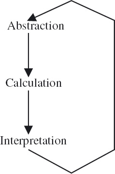
Figure 2.6: The abstraction–calculation–interpretation cycle.
x , y := y , x
swaps the values of x and y. (Variables x and y can have any type so long as it is the same for both.) Suppose f is a binary function of the appropriate type. Name the property that f should have in order that f(x,y) is an invariant of the assignment.

If you are unable to answer this question, read Section 12.5 on algebraic properties of binary operators.
(a) Identify an invariant of the non-deterministic choice
m := m+6  m := m+15.
(Recall that an expression is an invariant of a non-deterministic choice exactly when it is an invariant of all components of the choice.)
(b) Generalise your answer to
m := m+j m := m+k
where j and k are arbitrary integers. Give a formal verification of your claim.
(c) Is your answer valid when j and/or k is 0 (i.e. one or both of the assignments is equivalent to skip)? What other extreme cases can you identify?
To anwer this question, review Section 15.4. Only elementary properties are needed.
Exercise 2.8 When an assignment involves several variables, we can seek invariants that combine different subsets of the set of variables. For example, the assignment
m , n := m+2 , n+3
has invariants m mod 2, n mod 3 and 3×m − 2×n. This is what we did in Section 2.4 when we disregarded the variable w and considered only the variables b, d and  .
.
Consider the following non-deterministic choice:
m , n := m+1 , n+2 n , p := n+1 , p+3.
Identify as many (non-trivial) invariants as you can. (Begin by listing invariants of the individual assignments.)
Exercise 2.9 Consider the non-deterministic choice discussed in Section 2.4:
d , b , w := d+1 , b+3 , w+1 , b , w := +1 , b+1 , w+3.
There we verified that b − 3×d − is an invariant of the choice. This exercise is about constructing invariants that are linear combinations of subsets of the variables. Apply the technique discussed in Section 2.2: postulate that some linear combination of the variables is an invariant and then construct the coefficients. Because there are two assignments, you will get two equations in the unknowns.
(a) Determine whether a linear combination of two of the variables is an invariant of both assignments. (The answer is yes, but in an unhelpful way.)
(b) For each set of three variables, construct a (non-trivial) linear combination of the variables that is invariant under both assignments. (In this way, for b, d and , the linear combination b − 3×d − can be constructed. Similarly, an invariant linear combination of b, and w can be constructed, and likewise for b, d and w.
(c) What happens when you apply the technique to try to determine a linear combination of all four variables that is invariant?
2.6 BIBLIOGRAPHIC REMARKS
The empty-box problem was given to me by Wim Feijen. The problem of the black and white balls is from [Gri81]. The tetromino problems are from the 1999 Vierkant Voor Wiskunde calendar (see http://www.vierkantvoorwiskunde.nl/puzzels/). Vierkant Voor Wiskunde – foursquare for mathematics – is a foundation that promotes mathematics in Dutch schools. Their publications contain many examples of mathematical puzzles, both new and old. I have made grateful use of them throughout this text. Thanks go to Jeremy Weissman for suggestions on how to improve the presentation of the tetromino problems, some of which I have used. The domino and tumbler problems are old chestnuts. I do not know their origin.