Table of Contents for

Algorithmic Problem Solving

A requirement is that the size is a non-negative, whole number: thus 0, 1, 2, 3, etc. We use the term natural number for a non-negative, whole number. A word of warning: mathematicians often exclude the number 0 from the natural numbers. For typical real-life computing problems, however, it is very important that 0 should be included, making a break with tradition imperative. (For example, an internet search may yield 0 matches. A robot that processes search information must be programmed to deal with such a possibility.) Very occasionally, problems of size 0 do not make sense. In such cases the basis of the induction is problems of size 1. More generally, the basis may be problems of size n₀, for some number n₀; induction then provides a solution for all instances of size at least n₀.

Textbook problems are often presented in a way that makes the size parameter obvious, but this need not always be the case. For example, a given problem might involve a chessboard, which has 64 squares. There are several ways in which the problem might be generalised. The problem might be generalised to a class of problems where there are instances for each number n; the given problem is an instance such that n is 64. Such a generalisation takes no account of the structure of a chessboard. A second generalisation might exploit the fact that a chessboard is square: a class of problems is identified where an instance is an n×n board, for some n. The “size” of an instance of the class is then n (and not n²), and the size of the specific chessboard problem is 8. A third generalisation might depend on the fact that 8 is a power of 2; the class of problems is then restricted to square boards where the length of a side is 2ⁿ. In this case, the chessboard problem would have “size” 3 (because 8 = 2³).

6.1 EXAMPLE PROBLEMS

All the following problems can be solved by induction. In the first, the size is the number of lines. In the second and third problems, it is explicitly given by the parameter n. In each case, the basis should be easy. You then have to solve the induction step. We discuss each problem in turn in coming sections.

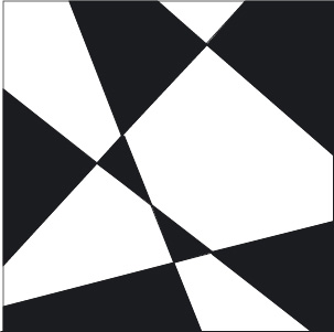
Figure 6.1: Black and white colouring.

1. Cutting the Plane   A number of straight lines are drawn across a sheet of paper, each line extending all the way from from one border to another (see Figure 6.1). In this way, the paper is divided into a number of regions.

Show that it is possible to colour each region black or white so that no two adjacent regions have the same colour (i.e. so that the two regions on opposite sides of any line segment have different colours).

2. Triominoes   A square piece of paper is divided into a grid of size 2ⁿ×2ⁿ, where n is a natural number.¹ The individual squares are called grid squares. One grid square is covered, and the others are left uncovered. A triomino is an L-shape made of three grid squares. Figure 6.2 shows, on the left, an 8×8 grid with one square covered. On the right is a triomino.

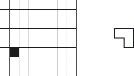
Figure 6.2: Triomino problem.

Show that it is possible to cover the remaining squares with (non-overlapping) triominoes. (Figure 6.3 shows a solution in one case.)

Note that the case n = 0 should be included in your solution.

3. Trapeziums   An equilateral triangle, with side of length 3n for some natural number n, is made of smaller equilateral triangles. Figure 6.4 shows the case where n is 2.

A bucket-shaped trapezium, shown on the right of Figure 6.4, is made from three equilateral triangles.

Show that it is possible to cover the remaining triangles with (non-overlapping) trapeziums. See Figure 6.5 for the solution in the case where n is 2.

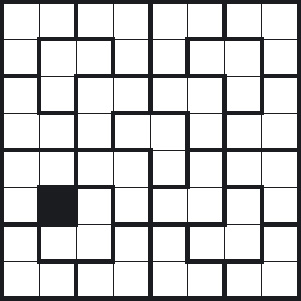
Figure 6.3: Triomino problem: solution to Figure 6.2.

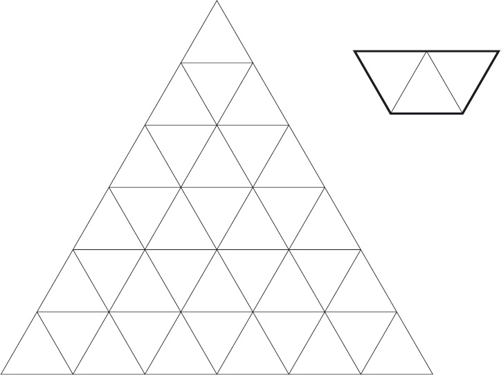
Figure 6.4: A pyramid of equilateral triangles and a trapezium.

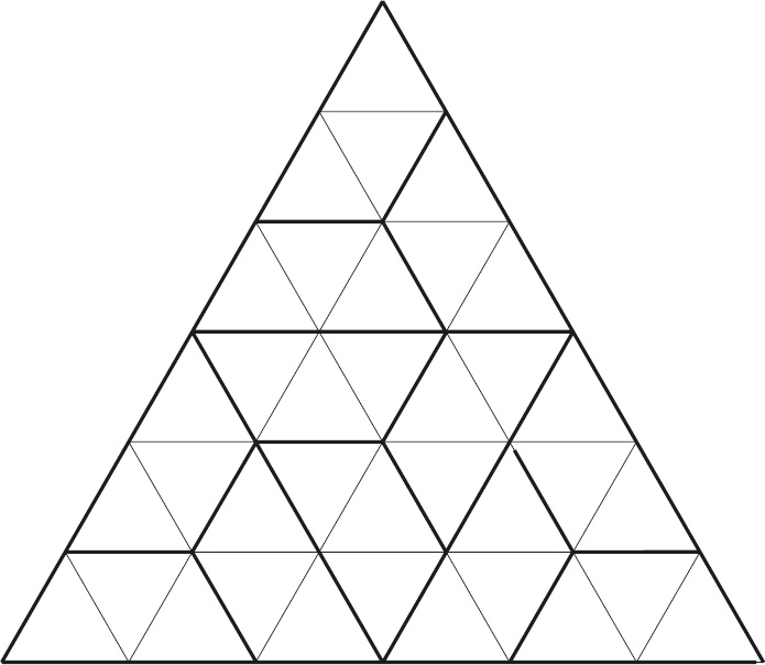
Figure 6.5: Solution to Figure 6.4.

Additional examples, such as fake-coin detection and the Tower of Hanoi problem, are discussed in later chapters.

6.2 CUTTING THE PLANE

Recall the statement of the problem:

A number of straight lines are drawn across a sheet of paper, each line extending all the way from one border to another (see Figure 6.1). In this way, the paper is divided into a number of regions. Show that it is possible to colour each region black or white so that no two adjacent regions have the same colour (i.e. so that the two regions on opposite sides of any line segment have different colours).

For this problem, the number of lines is an obvious measure of the “size” of the problem. The goal is, thus, to solve the problem “by induction on the number of lines”. This means that we have to show how to solve the problem when there are zero lines – this is the “basis” of the induction – and when there are n+1 lines, where n is an arbitrary number, assuming that we can solve the problem when there are n lines – this is the induction step.

For brevity, we call a colouring of the regions with the property that no two adjacent regions have the same colour a satisfactory colouring.

The case where there are zero lines is easy. The sheet of paper is divided into one region, and this can be coloured black or white, either colouring meeting the conditions of a solution (because there is no pair of adjacent regions).

For the induction step, we assume that a number of lines have been drawn on the sheet of paper, and the different regions have been coloured black or white so that no two adjacent regions have the same colour. This assumption is called the induction hypothesis. We now suppose that an additional line is drawn on the paper. This will divide some of the existing regions into two; such pairs of regions will have the same colour, and so the existing colouring is not satisfactory. Figure 6.6 is an example. The plane has been divided into 12 regions by five lines, and the regions coloured black and white, as required. An additional line, shown dashed for clarity, has been added. This has had the effect of dividing four of the regions into two, thus increasing the number of regions by four. On either side of the dashed line, the regions have the same colour. Elsewhere, adjacent regions have different colours. The task is to show how to modify the colouring so that it does indeed become a satisfactory solution.

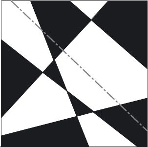
Figure 6.6: Cutting the plane. Additional line shown dashed.

The key to a solution is to note that inverting the colours of any satisfactory colouring (i.e. changing a black region to white, and vice versa) also gives a satisfactory colouring. Now, the additional line divides the sheet of paper into two regions. Let us call these regions the left and right regions. (By this choice of names, we do not imply that the additional line must be from top to bottom of the page. It is just a convenient, easily remembered, way of naming the regions.) Note that the assumed colouring is a satisfactory colouring of the left region and of the right region. In order to guarantee that, either side of the additional line, all regions have opposite colour, choose, say, the left region, and invert all the colours in that region. This gives a satisfactory colouring of the left region (because inverting the colours of a satisfactory colouring gives a satisfactory colouring). It also gives a satisfactory colouring of the right region (because the colouring has not changed, and was satisfactory already). Also, the colouring of adjacent regions at the boundary of the left and right regions is satisfactory, because they have changed from being the same to being different.

Figure 6.7 shows the effect on our example. Grey has been used instead of black in order to make the inversion of the colours more evident.

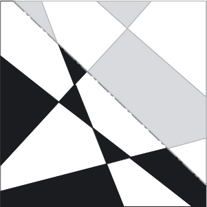
Figure 6.7: Cutting the plane. The colours are inverted to one side of the additional line (black is shown as grey to make clear which colours have changed).

This completes the induction step. In order to apply the construction to an instance of the problem with, say, seven lines, we begin by colouring the whole sheet of paper. Then the lines are added one by one. Each time a line is added, the existing colouring is modified as prescribed in the induction step, until all seven lines have been added.

The algorithm is non-deterministic in several ways. The initial colouring of the sheet of paper (black or white) is unspecified. The ordering of the lines (which to add first, which to add next, etc.) is also unspecified. Finally, which region is chosen as the “left” region, and which the “right” region is unspecified. This means that the final colouring may be achieved in lots of different ways. But that does not matter. The final colouring is guaranteed to be “satisfactory”, as required in the problem specification.

6.3 TRIOMINOES

As a second example of an inductive construction, let us consider the triomino problem posed in Section 6.1. Recall the statement of the problem:

A square piece of paper is divided into a grid of size 2ⁿ×2ⁿ, where n is a natural number. The individual squares are called grid squares. One grid square is covered, and the others are left uncovered. A triomino is an L-shape made of three grid squares. Show that it is possible to cover the remaining squares with (non-overlapping) triominoes.

The measure of the “size” of instances of the problem in this case is the number n. We solve the problem by induction on n.

The base case is when n equals 0. The grid then has size 2⁰×2⁰, that is, 1×1. That is, there is exactly one square. This one square is inevitably the one that is covered, leaving no squares uncovered. It takes 0 triominoes to cover no squares! This, then, is how the base case is solved.

Now consider a grid of size 2ⁿ⁺¹×2ⁿ⁺¹. Make the induction hypothesis that it is possible to cover any grid of size 2ⁿ×2ⁿ with triominoes if, first, an arbitrary grid square has been covered. We have to show how to exploit this hypothesis in order to cover a grid of size 2ⁿ⁺¹×2ⁿ⁺¹ of which one square has been covered.

A grid of size 2ⁿ⁺¹×2ⁿ⁺¹ can be subdivided into four grids each of size 2ⁿ×2ⁿ, simply by drawing horizontal and vertical dividing lines through the middle of each side (see Figure 6.8). Let us call the four grids the bottom-left, bottom-right, top-left, and top-right grids. One grid square is already covered. This square will be in one of the four sub-grids. We may assume that it is in the bottom-left grid. (If not, the entire grid can be rotated about the centre so that it does become the case.)

The bottom-left grid is thus a grid of size 2ⁿ×2ⁿ of which one square has been covered. By the induction hypothesis, the remaining squares in the bottom-left grid can be covered with triominoes. This leaves us with the task of covering the bottom-right, top-left and top-right grids with triominoes.

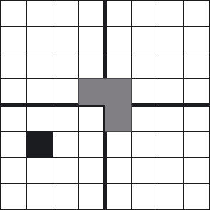
Figure 6.8: Triomino problem: inductive step. The grid is divided into four sub-grids. The covered square, shown in black, identifies one sub-grid. A triomino, shown in grey, is placed at the junction of the other three grids. The induction hypothesis is then used to cover all four sub-grids with triominoes.

None of the squares in these three grids is covered, as yet. We can apply the induction hypothesis to them if just one square in each of the three is covered. This is done by placing a triomino at the junction of the three grids, as shown in Figure 6.8.

Now, the inductive hypothesis is applied to cover the remaining squares of the bottom-right, top-left and top-right grids with triominoes. On completion of this process, the entire 2ⁿ⁺¹×2ⁿ⁺¹ grid has been covered with triominoes.

6.4 LOOKING FOR PATTERNS

In Sections 6.2 and 6.3, we have seen how induction is used to solve problems of a given “size”. Technically, the process we described is called “mathematical induction”; “induction”, as it is normally understood, is more general.

“Induction”, as used in, for example, the experimental sciences, refers to a process of reasoning whereby general laws are inferred from a collection of observations. A famous example of induction is the process that led Charles Darwin to formulate his theory of evolution by natural selection, based on his observations of plant and animal life in remote parts of the world. In simple terms, induction is about looking for patterns.

Laws formulated by a process of induction go beyond the knowledge on which they are based, thus introducing inherently new knowledge. In the experimental sciences, however, such laws are only probably true; they are tested by the predictions they make, and may have to be discarded if the predictions turn out to be false. In contrast, deduction is the process of inferring laws from existing laws, whereby the deductions made are guaranteed to be true provided that the laws on which they are based are true. In a sense, laws deduced from existing laws add nothing to our stock of knowledge since they are, at best, simply reformulations of existing knowledge.

Mathematical induction is a combination of induction and deduction. It is a process of looking for patterns in a set of observations, formulating the patterns as conjectures, and then testing whether the conjectures can be deduced from existing knowledge. Guess-and-verify is a brief way of summarising mathematical induction. (Guessing is the formulation of a conjecture; verification is the process of deducing whether the guess is correct.)

Several of the matchstick games studied in Chapter 4 provide good examples of mathematical induction. Recall, for example, the game discussed in Section 4.2.2: there is one pile of matches from which it is allowed to remove one or two matches. Exploring this game, we discovered that a pile with 0, 3 or 6 matches is a losing position, and piles with 1, 2, 4, 5, 7 and 8 matches are winning positions. There seems to be a pattern in these numbers: losing positions are the positions in which the number of matches are a multiple of 3, and winning positions are the remaining positions. This is a conjecture about all positions made from observations on just nine positions. However, we can verify that the conjecture is true by using mathematical induction to construct a winning strategy.

In order to use induction, we measure the “size” of a pile of matches not by the number of matches but by the number of matches divided by 3, rounded down to the nearest natural number. So, the “size” of a pile of 0, 1 or 2 matches is 0, the “size” of a pile of 3, 4 or 5 matches is 1, and so on. The induction hypothesis is that a pile of 3n matches is a losing position, and a pile of 3n + 1 or 3n + 2 matches is a winning position.

The basis for the induction is when n equals 0. A pile of 0 matches is, indeed, a losing position because, by definition, the game is lost when it is no longer possible to move. A pile of 1 or 2 matches is a winning position because the player can remove the matches, leaving the opponent in a losing position.

Now, for the induction step, we assume that a pile of 3n matches is a losing position, and a pile of 3n + 1 or 3n + 2 matches is a winning position. We have to show that a pile of 3(n+1) matches is a losing position, and a pile of 3(n+1) + 1 or 3(n+1) + 2 matches is a winning position.

Suppose there are 3(n+1) matches. The player, whose turn it is, must remove 1 or 2 matches, leaving either 3(n+1) − 1 or 3(n+1) − 2 behind. That is, the opponent is left with either 3n + 2 or 3n + 1 matches. But, by the induction hypothesis, this leaves the opponent in a winning position. Hence, the position in which there are 3(n+1) matches is a losing position.

Now, suppose there are 3(n+1) + 1 or 3(n+1) + 2 matches. By taking 1 match in the first case, and 2 matches in the second case, the player leaves the opponent in a position where there are 3(n+1) matches. This we now know to be a losing position. Hence, the positions in which there are 3(n+1) + 1 or 3(n+1) + 2 are both winning positions.

This completes the inductive construction of the winning moves, and thus verifies the conjecture that a position is a losing position exactly when the number of matches is a multiple of 3.

6.5 THE NEED FOR PROOF

When using induction, it is vital that any conjecture is properly verified. It is too easy to extrapolate from a few cases to a more general claim that is not true. Many conjectures turn out to be false; only by subjecting them to the rigours of proof can we be sure of their validity. This section is about a non-trivial example of a false conjecture.

Suppose n points are marked on the circumference of a circular cake and then the cake is cut along the chords joining them. The points are chosen in such a way that all intersection points of pairs of chords are distinct. The question is, in how many portions does this cut the cake?

Figure 6.9 shows the case when n is 1, 2, 3 or 4. The number of portions is successively 1, 2, 4 and 8. This suggests that the number of portions, for arbitrary n, is 2ⁿ⁻¹. Indeed, this conjecture is supported by the case that n = 5. (We leave the reader to draw the figure.) In this case, the number of portions is 16, which is 2⁵⁻¹. However, for n = 6, the number of portions is 31! (See Figure 6.10.) Note that n = 6 is the first case in which the points are not allowed to be placed at equal distances around the perimeter.

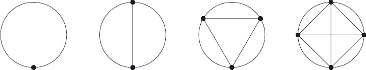
Figure 6.9: Cutting the cake.

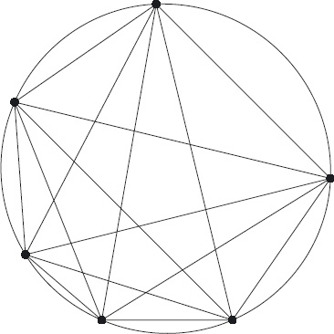
Figure 6.10: Cutting the cake: the case n = 6. The number of portions is 31, not 2⁶⁻¹.

Had we begun by considering the case where n = 0, suspicions about the conjecture would already have been raised – it does not make sense to say that there are 2⁰⁻¹ portions, even though cutting the cake as stated does make sense! The easy, but inadequate, way out is to dismiss this case, and impose the requirement that n is different from 0. The derivation of the correct formula for the number of portions is too complicated to discuss here, but it does include the case where n equals 0!

6.6 FROM VERIFICATION TO CONSTRUCTION

In mathematical texts, induction is often used to verify known formulae. Verification is important but has a major drawback – it seems that a substantial amount of clairvoyance is needed to come up with the formula that is to be verified. And, if one’s conjecture is wrong, verification gives little help in determining the correct formula.

Induction is sometimes used in computing science as a verification principle, but it is most important as a fundamental principle in the construction of computer programs. This section introduces the use of induction in the construction of mathematical formulae.

The problem we consider is how to determine a closed formula for the sum of the kth powers of the first n natural numbers.

A well-known formula gives the sum of the natural numbers from 1 thru n :

Two other exercises, often given in mathematical texts, are to verify that

and

As well as being good examples of the strength of the principle of mathematical induction, the examples also illustrate the weakness of verification: the technique works if the answer is known, but what happens if the answer is not already known! Suppose, for example, that you are now asked to determine a closed formula for the sum of the 4th powers of the first n numbers,

1⁴+ 2⁴+ . . . + n⁴ = ?.

How would you proceed? Verification, using the principle of mathematical induction, does not seem to be applicable unless we already know the right-hand side of the equation. Can you guess what the right side would be in this case? Can you guess what the right side would be if the power, 4, is replaced by, say, 27? Almost certainly not!

Constructing solutions to non-trivial problems involves a creative process. This means that a certain amount of guesswork is necessary, and trial and error cannot be completely eliminated. Reducing the guesswork to a minimum, replacing it by mathematical calculation is the key to success.

Induction can be used to construct closed formulae for such summations. The general idea is to seek a pattern, formulate the pattern in precise mathematical terms and then verify the pattern. The key to success is simplicity. Do not be over-ambitious. Leave the work to mathematical calculation.

A simple pattern in the formulae displayed above is that, for m equal to 1, 2 and 3, the sum of the mth powers of the first n numbers is a polynomial in n of degree m+1. (The sum of the first n numbers is a quadratic function of n, the sum of the first n squares is a cubic function of n, and the sum of the first n cubes is a quartic function of n.) This pattern is also confirmed in the (oft-forgotten) case that m is 0:

1⁰ + 2⁰ + . . . + n⁰ = n.

A strategy for determining a closed formula for, say, the sum of the fourth powers is thus to guess that it is a fifth-degree polynomial in n and then use induction to calculate the coefficients. The calculation in this case is quite long, so let us illustrate the process by showing how to construct a closed formula for 1 + 2 + . . . + n. (Some readers will already know a simpler way of deriving the formula in this particular case. If this is the case, then bear with us. The method described here is more general.)

We conjecture that the required formula is a second-degree polynomial in n, say a + bn + cn² and then calculate the coefficients a, b and c. Here is how the calculation goes.

For brevity, let us use S(n) to denote

1 + 2 + . . . + n.

We also use P(n) to denote the proposition

S(n) = a + bn + cn².

Then,

       P(0)
=             {          definition of P   }
       S(0) = a+b × 0+c × 0²
=            {            S(0) = 0 (the sum of an empty set of numbers
                            is zero) and arithmetic }
       0 = a

So the basis of the induction has allowed us to deduce that a, the coefficient of n⁰, is 0. Now, we calculate b and c. To do so, we make the induction hypothesis that 0 ≤ n and P(n) is true. Then

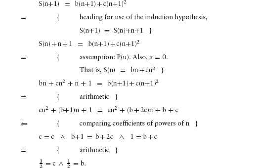
From the conjecture that the sum of the first n numbers is a quadratic in n, we have thus calculated that

Extrapolating from this calculation, one can see that it embodies an algorithm to express 1^m + 2^m + . . . + n^m as a polynomial function for any given natural number m. The steps in the algorithm are: postulate that the summation is a polynomial in n with degree m+1. Use the principle of mathematical induction together with the facts that S(0) is 0 and S(n+1) is S(n)+(n+1)^m (where S(n) denotes 1^m + 2^m + . . . + n^m) to determine a system of simultaneous equations in the coefficients. Finally, solve the system of equations.

It is worth remarking here that, in the case of the sum 1 + 2 + . . . + n, there is an easier way to derive the correct formula. Simply write down the required sum

1 + 2 + . . . + n,

and immediately below it

n + n−1 + . . . + 1.

Then add the two rows together:

n+1 + n+1 + . . . + n+1.

From the fact that there are n occurrences of n+1 we conclude that the sum is However, this method cannot be used for determining 1^m + 2^m + . . . + n^m for m greater than 1.

6.8 BIBLIOGRAPHIC REMARKS

All the problems in this chapter are very well known. I have not attempted to trace their origin. The trapezium problems were suggested by an anonymous reviewer.

The triomino and trapezium problems are instances of so-called tiling problems. Generally the form that such problems take is to determine whether or not it is possible to cover a given area using tiles of a given shape. Some tiling problems have an ad hoc solution: the problem cannot be generalised to a class of problems. When a generalisation is possible, and the problem is solvable, we seek an algorithm to perform the tiling. Tiling problems can be very hard to solve and finding the right generalisation can often be critical to success.

¹ Recall that the natural numbers are the numbers 0, 1, 2, etc.