Table of Contents for
Algorithmic Problem Solving
 Algorithmic Problem Solving
Published by
John Wiley & Sons, 2011
Algorithmic Problem Solving
Published by
John Wiley & Sons, 2011
- Coverpage
- Algorithmic Problem Solving
- Titlepage
- Copyright
- Preface
- Contents
- PART I: Algorithmic Problem Solving
- CHAPTER 1: Introduction
- CHAPTER 2: Invariants
- CHAPTER 3: Crossing a River
- CHAPTER 4: Games
- CHAPTER 5: Knights and Knaves
- CHAPTER 6: Induction
- CHAPTER 7: Fake-Coin Detection
- CHAPTER 8: The Tower of Hanoi
- CHAPTER 9: Principles of Algorithm Design
- CHAPTER 10: The Bridge Problem
- CHAPTER 11: Knight’s Circuit
- PART II: Mathematical Techniques
- CHAPTER 12: The Language of Mathematics
- CHAPTER 13: Boolean Algebra
- CHAPTER 14: Quantifiers
- CHAPTER 15: Elements of Number Theory
- CHAPTER 16: Relations, Graphs and Path Algebras
- Solutions to Exercises
- References
- Index

This chapter is about how to win some simple two-person games. The goal is to have some method (i.e. “algorithm”) for deciding what to do so that the eventual outcome is a win.
The key to developing a winning strategy is the recognition of invariants. So, in essence, this chapter is a continuation of Chapter 2. The chapter is also about trying to identify and exploit structure in problems. In this sense, it introduces the importance of algebra in problem solving.
The next section introduces a number of games with matchsticks, in order to give the flavour of the games that we consider. Following it, we develop a method of systematically identifying winning and losing positions in a game (assuming a number of simplifying constraints on the rules of the game). A winning strategy is then what we call “maintaining an invariant”. “Maintaining an invariant” is an important technique in algorithm development. Here, it will mean ensuring that the opponent is always placed in a position from which losing is inevitable.
4.1 MATCHSTICK GAMES
A matchstick game is played with one or more piles of matches. Two players take turns to make a move. Moves involve removing one or more matches from one of the piles, according to a given rule. The game ends when it is no longer possible to make a move. The player whose turn it is to move is the loser, and the other player is the winner.
A matchstick game is an example of an impartial, two-person game with complete information. “Impartial” means that rules for moving apply equally to both players. (Chess, for example, is not impartial, because white can move only white pieces, and black can move only black pieces.) “Complete information” means that both players know the complete state of the game. In contrast, in card games like poker, each player does not know the cards held by the other player; the players have incomplete information about the state of the game.
A winning position is one from which a perfect player is always assured of a win. A losing position is one from which a player can never win, when playing against a perfect player. A winning strategy is an algorithm for choosing moves from winning positions that guarantees a win.
As an example, suppose there is one pile of matches, and an allowed move is to remove 1 or 2 matches. The losing positions are the positions where the number of matches is a multiple of 3 (i.e. the number of matches is 0, 3, 6, 9, etc.). The remaining positions are the winning positions. If n is the number of matches in such a position (i.e. n is not a multiple of 3), the strategy is to remove n mod 3 matches.1 This is either 1 or 2, so the move is valid. The opponent is then put in a position where the number of matches is a multiple of 3. This means that there are either 0 matches left, in which case the opponent loses, or any move they make will result in there again being a number of matches remaining that is not a multiple of 3.
In an impartial game that is guaranteed to terminate no matter how the players choose their moves (i.e. the possibility of stalemate is excluded), it is always possible to characterise the positions as either winning or losing positions. The following exercises ask you to do this in specific cases.
1. There is one pile of matches. Each player is allowed to remove 1 match.
What are the winning positions?
2. There is one pile of matches. Each player is allowed to remove 0 matches, but must remove at least 1 match.
What are the winning positions?
3. Can you see a pattern in the last two problems and the example discussed above (in which a player is allowed to remove 1 or 2 matches)?
In other words, can you see how to win a game in which an allowed move is to remove at least 1 and at most N matches, where N is some number fixed in advance?
4. There is one pile of matches. Each player is allowed to remove 1, 3 or 4 matches.
What are the winning positions and what is the winning strategy?
5. There is one pile of matches. Each player is allowed to remove 1, 3 or 4 matches, except that it is not allowed to repeat the opponent’s last move. (So, if, say, your opponent removes 1 match, your next move must be to remove 3 or 4 matches.)
What are the winning positions and what is the winning strategy?
6. There are two piles of matches. A move is to choose one pile and, from that pile, remove 1, 2 or 3 matches.
What are the winning positions and what is the winning strategy?
7. There are two piles of matches. A move is to choose one pile; from the left pile 1, 2 or 3 matches may be removed, and from the right pile 1 thru 7 matches may be removed.
What are the winning positions and what is the winning strategy?
8. There are two piles of matches. A move is to choose one pile; from the left pile, 1, 3 or 4 matches may be removed, and, from the right pile, 1 or 2 matches may be removed.
What are the winning positions and what is the winning strategy?
4.2 WINNING STRATEGIES
In this section, we formulate what is required of a winning strategy. We begin with the simple matchstick game where a move is to remove one or two matches from a single pile of matches; we show how to search systematically through all the positions of the game, labelling each as either a winning or a losing position. Although a brute-force search, and thus not practical for more complicated games, the algorithm does give a better understanding of what is involved and can be used as a basis for developing more efficient solutions in particular cases.
4.2.1 Assumptions
We make a number of assumptions about the game, in order that the search will work.
- We assume that the number of positions is finite.
- We assume that the game is guaranteed to terminate no matter how the players choose their moves.
The first assumption is necessary because a one-by-one search of the positions can never be complete if the number of positions is infinite. The second assumption is necessary because the algorithm relies on being able to characterise all positions as either losing or winning; we exclude the possibility that there are stalemate positions. Stalemate positions are ones from which the players can continue the game indefinitely, so that neither player can win.
4.2.2 Labelling Positions
The first step is to draw a directed graph depicting positions and moves in the game. Figure 4.1 is a graph of the matchstick game described at the beginning of Section 4.1 for the first nine positions.
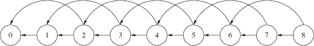
 Figure 4.1: Matchstick game. Players may take one or two matches at each turn.
A directed graph has a set of nodes and a set of edges. Each edge is from one node to another node. When graphs are drawn, nodes are depicted by circles, and edges are depicted by arrows pointing from the from node to the to node.
 Our assumptions on games (see Section 4.2.1) mean that the graph of a game is finite and acyclic. This in turn means that properties of the graph can be determined by a topological search of the graph. See Section 16.7 and, in particular, Section 16.7.1 for more on these important concepts.
The nodes in Figure 4.1 are labelled by the number of matches remaining in the pile. From the node labelled 0, there are no edges. It is impossible to move from the position in which no matches remain. From the node labelled 1, there is exactly one edge, to the node labelled 0. From the position in which one match remains, there is exactly one move that can be made, namely to remove the remaining match. From all other nodes, there are two edges. From the node labelled n, where n is at least 2, there is an edge to the node labelled n−1 and an edge to the node labelled n−2. That is, from a position in which the number of remaining matches is at least 2, one may remove one or two matches.
Having drawn the graph, we can begin labelling the nodes as either losing positions or winning positions. A player who finds themself in a losing position will inevitably lose, if playing against a perfect opponent. A player who finds themself in a winning position is guaranteed to win, provided the right choice of move is made at each turn.
The labelling rule has two parts, one for losing positions, the other for winning positions:
- A node is labelled losing if every edge from the node is to a winning position.
- A node is labelled winning if there is an edge from the node to a losing position.
At first sight, it may seem that it is impossible to begin to apply these rules; after all, the first rule defines losing positions in terms of winning positions, while the second rule does the reverse. It seems like a vicious circle! However, we can begin by labelling as losing positions all the nodes with no outgoing edges. This is because, if there are no edges from a node, the statement “every edge from the node is to a winning position” is true. It is indeed the case that all of the (non-existent) edges are to a winning position.
This is an instance of a general rule of logic. A statement of the form “every x has property p” is called a for-all quantification, or a universal quantification. Such a statement is said to be vacuously true when there are no instances of the “x” in the quantification. In a sense, the statement is “vacuous” (i.e. empty) because it is a statement about nothing.
A “quantification” extends a binary operator (a function on two values) to a collection of values. Summation is an example of a quantification: the binary operator is adding two numbers. In the case of universal quantification, the binary operator is logical “and”. See Chapter 14 for full details.
Returning to Figure 4.1, node 0 is labelled “losing” because there are no edges from it. It is indeed a losing position, because the rules of the game specify that a player who cannot make a move loses.
Next, nodes 1 and 2 are labelled “winning”, because, from each, there is an edge to 0, which we know to be a losing position. Note that the edges we have identified dictate the move that should be made from these positions if the game is to be won.
Now, node 3 is labelled “losing”, because both edges from node 3 are to nodes (1 and 2) that we have already labelled “winning”. From a position in which there are 3 matches remaining, every move is to a position starting from which a win is guaranteed. A player that finds themself in this position will eventually lose.
The process we have described repeats itself until all nodes have been labelled. Nodes 4 and 5 are labelled “winning”, then node 6 is labelled “losing”, then nodes 7 and 8 are labelled “winning”, and so on.
Figure 4.2 shows the state of the labelling process at the point that node 7 has been labelled but not node 8. The circles depicting losing positions are drawn with thick lines; the circles depicting winning positions are the ones from which there is an edge drawn with a thick line. These edges depict the winning move from that position.
Clearly, a pattern is emerging from this process: a losing position is one where the number of matches is a multiple of 3, and all others are winning positions. The winning strategy is to remove one or two matches so as to leave the opponent in a position where the number of matches is a multiple of 3.
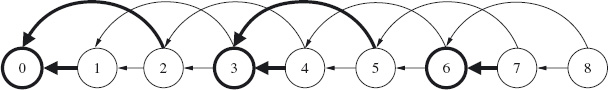
Figure 4.2: Labelling positions. Winning edges are indicated by thick edges.
4.2.3 Formulating Requirements
The terminology we use to describe the winning strategy is to “maintain” the property that the number of matches is a multiple of 3. In programming terms, we express this property using Hoare triples. Let n denote the number of matches in the pile. Then, the correctness of the winning strategy is expressed by the following annotated program segment:
{ n is a multiple of 3, and n ≠ 0 }
if 1 ≤ n → n := n−1  2 ≤ n → n := n−2
 fi
; { n is not a multiple of 3 }
n := n − (n mod 3)
{ n is a multiple of 3 }
This program segment has five components, each on a separate line. The first line, the precondition, expresses the assumption that execution begins from a position in which the number of matches is a multiple of 3 and is non-zero.
The second line uses a non-deterministic conditional statement2 to model an arbitrary move. Removing one match is allowed only if 1 ≤ n; hence, the statement n := n−1 is “guarded” by this condition. Similarly, removing two matches – modelled by the assignment n := n−2 – is “guarded” by the condition 2 ≤ n. At least one of these guards, and possibly both, is true because of the assumption that n ≠ 0.
The postcondition of the guarded command is the assertion “n is not a multiple of 3”. The triple comprising the first three lines thus asserts that if the number of matches is a multiple of 3, and a valid move is made that reduces the number of matches by one or two, then, on completion of the move, the number of matches is not a multiple of 3.
The fourth line of the sequence is the implementation of the winning strategy; specifically, remove n mod 3 matches. The fifth line is the final postcondition, which asserts that, after execution of the winning strategy, the number of matches is again a multiple of 3.
In summary, beginning from a state in which n is a multiple of 3, and making an arbitrary move, results in a state in which n is not a multiple of 3. Subsequently, removing n mod 3 matches results in a state in which n is again a multiple of 3.
In general, a winning strategy is obtained by characterising the losing positions by some property, losing say. The end positions (the positions where the game is over) must satisfy the property losing. The winning positions are then the positions that do not satisfy losing. For each winning position, one has to identify a way of calculating a losing position to which to move; the algorithm that is used is the winning strategy. More formally, the losing and winning positions and the winning strategy must satisfy the following specification.
{ losing position, and not an end position }
make an arbitrary (legal) move
; { winning position, i.e. not a losing position }
apply winning strategy
{ losing position }
In summary, a winning strategy is a way of choosing moves that divides the positions into two types, the losing positions and the winning positions, such that the following three properties hold:
- End positions are losing positions.
- From a losing position that is not an end position, every move is to a winning position. That is, every move falsifies the property of being a losing position.
- From a winning position, it is always possible to apply the winning strategy, resulting in a losing position. That is, it is always possible to choose a move that truthifies3 the property of being a losing position.
If both players are perfect, the winner is decided by the starting position. If the starting position is a losing position, the second player is guaranteed to win. And if the starting position is a winning position, the first player is guaranteed to win. The perfect player wins from a winning position by truthifying the invariant, thus placing the opponent in a losing position. Starting from a losing position, one can only hope that one’s opponent is not perfect, and will make a mistake.
We recommend that you now try to solve the matchstick-game problem when the rule is that any number of matches from 1 thru M may be removed at each turn. The number M is a natural number, fixed in advance. We recommend that you try to solve this general problem by first considering the case where M is 0. This case has a very easy solution, although it is a case that is very often neglected. Next, consider the case where M is 1. This case also has an easy solution, but slightly more complicated. Now, combine these two cases with the case where M is 2, which is the case we have just considered. Do you see a pattern in the solutions? If you do not see a pattern immediately, try a little harder. As a last resort, try working out the case where M is 3. (It is better to construct a table rather than draw a diagram. At this stage a diagram is becoming too complicated.) Then return to the cases where M is 0, 1 and 2 (in particular, the extreme cases 0 and 1) in order to check the pattern you have identified. Finally, formulate the correctness of the strategy by a sequence of assertions and statements, as we did above for the case where M is 2.
Exercise 4.1 (31st December Game) Two players alternately name dates. The winner is the player who names 31st December, and the starting date is 1st January.
Each part of this exercise uses a different rule for the dates that a player is allowed to name. For each, devise a winning strategy, stating which player should win. State also if it depends on whether the year is a leap year or not.
Hint: in principle, you have to determine for each of 365 days (or 366 in the case of a leap year) whether naming the day results in losing against a perfect player. In practice, a pattern soon becomes evident and the days in each month can be grouped together into winning and losing days. Begin by identifying the days in December that one should avoid naming.
(a) (Easy) A player can name the 1st of the next month, or increase the day of the month by an arbitrary amount. (For example, the first player begins by naming 1st February, or a date in January other than the 1st.)
(b) (Harder) A player can increase the day by one, leaving the month unchanged, or name the 1st of the next month.
4.3 SUBTRACTION - SET GAMES
A class of matchstick games is based on a single pile of matches and a (finite) set of numbers; a move is to remove m matches, where m is an element of the given set. A game in this class is called a subtraction-set game, and the set of numbers is called the subtraction set.
The games we have just discussed are examples of subtraction-set games; if the rule is that 1 thru M matches may be removed at each turn, the subtraction set is {1..M}. More interesting examples are obtained by choosing a subtraction set with less regular structure.
For any given subtraction set, the winning and losing positions can always be computed. We exemplify the process in this section by calculating the winning and losing positions when the allowed moves are:
- remove one match,
- remove three matches,
- remove four matches.
In other words, the subtraction set is {1, 3, 4}.
Positions in the game are given by the number of matches in the pile. We refer to the positions using this number. So, “position 0” means the position in which there are no matches remaining in the pile, “position 1” means the position in which there is just one match in the pile, and so on.
Beginning with position 0, and working through the positions one by one, we identify whether each position is a winning position using the rules that
- a position is a losing position if every move from it is to a winning position, and
- a position is a winning position if there is a move from it to a losing position.
The results are entered in a table. The top half of Table 4.1 shows the entries when the size of the pile is at most 6. The first row is the position, and the second row shows whether or not it is a winning (W) or losing position (L). In the case where the position is a winning position, the third row shows the number of matches that should be removed in order to move from the position to a losing position. For example, 2 is a losing position because the only move from 2 is to 1; positions 3 and 4 are winning positions because from both a move can be made to 0. Note that there may be a choice of winning move. For example, from position 3 there are two winning moves – remove 3 matches to move to position 0, or remove 1 match to move to position 2. It suffices to enter just one move in the bottom row of the table.
Continuing this process, we get the next seven entries in the table: see the bottom half of Table 4.1. Comparing the two halves of the table, we notice that the pattern of winning and losing positions repeats itself. Once the pattern begins repeating in this way, it will continue to do so forever. We may therefore conclude that, for the subtraction set {1, 3, 4}, whether or not the position is a winning position can be determined by computing the remainder, r say, after dividing the number of matches by 7. If r is 0 or 2, the position is a losing position. Otherwise, it is a winning position. The winning strategy is to remove 1 match if r is 1, remove 3 matches if r is 3 or 5, and remove 4 matches if r is 4 or 6.
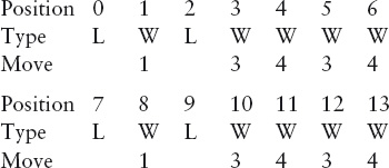
Table 4.1: Winning (W) and losing (L) positions for subtraction set {1, 3, 4}.
The repetition in the pattern of winning and losing positions that is evident in this example is a general property of subtraction-set games, with the consequence that, for a given subtraction set, it is always possible to determine for an arbitrary position whether or not it is a winning position (and, for the winning positions, a winning move). The following argument gives the reason why.
Suppose a subtraction set is given. Since the set is assumed to be finite, it must have a largest element. Let this be M. Then, from each position, there are at most M moves. For each position k, let W(k) be true if k is a winning position, and false otherwise. When k is at least M, W(k) is completely determined by the sequence W(k−1), W(k−2), . . ., W(k−M). Call this sequence s(k). Now, there are only 2M different sequences of booleans of length M. As a consequence, the sequence s(M+1), s(M+2), s(M+3), . . . must eventually repeat, and it must do so within at most 2M steps. That is, for some j and k, with M ≤ j < k < M+2M, we must have s(j) = s(k). It follows that W(j) = W(k) and the sequence W repeats from the kth position onwards.
For the example above, this analysis predicts that the winning–losing pattern will repeat from the 20th position onwards. In fact, it begins repeating much earlier. Generally, we can say that the pattern of win–lose positions will repeat at position 2M+M, or before. To determine whether an arbitrary position is a winning or losing position involves computing the status of each position k, for successive values of k, until a repetition in s(k) is observed. If the repetition occurs at position R, then, for an arbitrary position k, W(k) equals W(k mod R).
Exercise 4.2 Suppose there is one pile of matches. In each move, 2, 5 or 6 matches may be removed. (That is, the subtraction set is {2, 5, 6}.)
(a) For each n, 0 ≤ n < 22, determine whether a pile of n matches is a winning or losing position.
(b) Identify a pattern in the winning and losing positions. Specify the pattern by giving precise details of a boolean function of n that determines whether a pile of n matches is a winning position or not. Verify the pattern by constructing a table showing how the function’s value changes when a move is made.
Exercise 4.3 This exercise is challenging; its solution involves thinking beyond the material presented in the rest of the chapter.
Figure 4.3 shows a variant of snakes and ladders. In this game, there is just one counter. The two players take it in turn to move the counter at most four spaces forward. The start is square 1 and the finish is square 25; the winner is the first to reach the finish. As in the usual game of snakes and ladders, if the counter lands on the head of a snake, it falls down to the tail of the snake; if the counter lands at the foot of a ladder, it climbs to the top of the ladder.
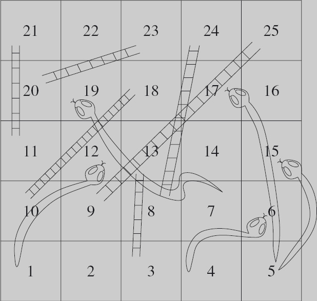
 Figure 4.3: Snakes and ladders. Players take it in turn to move the counter at most four spaces forward.
(a) List the positions in this game. (These are not the same as the squares. Think carefully about squares linked by a snake or a ladder.)
(b) Identify the winning and losing positions. Use the rule that a losing position is one from which every move is to a winning position, and a winning position is one from which there is a move to a losing position.
(c) Some of the positions cannot be identified as winning or losing in this way. Explain why.
4.4 SUMS OF GAMES
In this section we look at how to exploit the structure of a game in order to compute a winning strategy more effectively.
The later examples of matchstick games in Section 4.1 have more than one pile of matches. When a move is made, one of the piles must first be chosen; then, matches may be removed from the chosen pile according to some prescribed rule, which may differ from pile to pile. The game is thus a combination of two games; this particular way of combining games is called summing the games.
In general, given two games each with its own rules for making a move, the sum of the games is the game described as follows. For clarity, we call the two games the left and the right game. A position in the sum game is the combination of a position in the left game and a position in the right game. A move in the sum game is a move in one of the games.
Figure 4.4 is an example of the sum of two games. Each graph represents a game, where the positions are represented by the nodes, and the moves are represented by the edges. Imagine a coin placed on a node. A move is then to displace the coin along one of the edges to another node. The nodes in the left graph and right graphs are named by capital letters and small letters, respectively, so that we can refer to them later.
In the “sum” of the games, two coins are used, one coin being placed over a node in each of the two graphs. A move is then to choose one of the coins, and displace it along an edge to another node. Thus, a position in the “sum” of the games is given by a pair Xx where “X” names a node in the left graph, and “x” names a node in the right graph; a move has the effect of changing exactly one of “X” or “x”.
Both the left and right games in Figure 4.4 are unstructured; consequently, the brute-force search procedure described in Section 4.2.2 is unavoidable when determining their winning and losing positions. However, the left game in Figure 4.4 has 15 different positions, and the right game has 11; thus, the sum of the two games has 15×11 different positions. For this game, and for sums of games in general, a brute-force search is highly undesirable. In this section, we study how to compute a winning strategy for the sum of two games. We find that the computational effort is the sum (in the usual sense of addition of numbers) of the effort required to compute winning and losing positions for the component games, rather than the product. We find, however, that it is not sufficient to know just the winning strategy for the individual games. Deriving a suitable generalisation forms the core of the analysis.
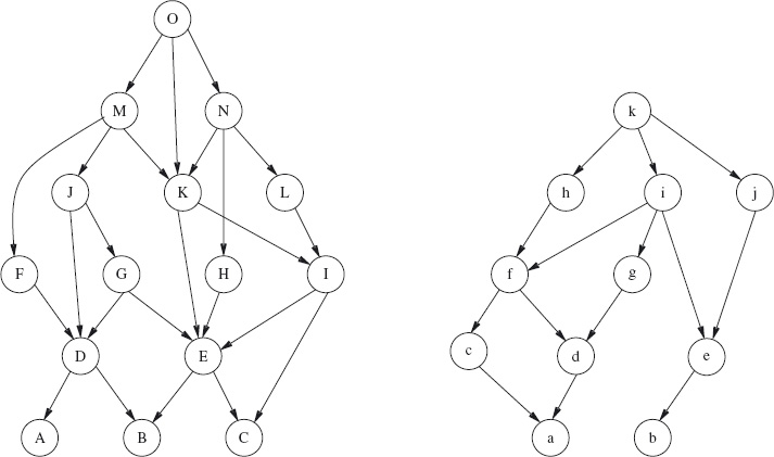
Figure 4.4: A sum game. The left and right games are represented by the two graphs. A position is a pair Xx where “X” is the name of a node in the left graph, and “x” is the name of a node in the right graph. A move changes exactly one of X or x.
The set of positions in a sum game is the cartesian product of the sets of positions in the component games. This explains why the number of positions in the sum game is the product of the number of positions in the component games. See Section 12.4.1.
4.4.1 A Simple Sum Game
We begin with a very simple example of the sum of two games. Suppose there are two piles of matches. An allowed move is to choose any one of the piles and remove at least one match from the chosen pile. Otherwise, there is no restriction on the number of matches that may be removed. As always, the game is lost when a player cannot make a move.
This game is the “sum” of two instances of the same, very, very simple, game: given a (single) pile of matches, a move is to remove at least one match from the pile. In this simple game, the winning positions are, obviously, the positions in which the pile has at least one match, and the winning strategy is to remove all the matches. The position in which there are no matches remaining is the only losing position.
It quickly becomes clear that knowing the winning strategy for the individual games is insufficient to win the sum of the games. If a player removes all the matches from one pile – that is, applies the winning strategy for the individual game – the opponent wins by removing the remaining matches in the other pile.
The symmetry between left and right allows us to easily spot a winning strategy. Suppose we let m and n denote the number of matches in the two piles. In the end position, there is an equal number of matches in both piles, namely 0. That is, in the end position, m = n = 0. This suggests that the losing positions are given by m = n. This is indeed the case. From a position in which m = n and a move is possible (i.e. either 1 ≤ m or 1 ≤ n), any move will be to a position where m ≠ n. Subsequently, choosing the pile with the larger number of matches, and removing the excess matches from this pile, will restore the property that m = n.
Formally, the correctness of the winning strategy is expressed by the following sequence of assertions and program statements.
{ m = n ∧ (m ≠ 0 ∨ n ≠ 0) }
if 1 ≤ m → reduce m
1 ≤ n → reduce n
fi
; { m ≠ n }
if m < n → n := n − (n−m)
n < m → m := m − (m−n)
fi
{ m = n }
The non-deterministic choice between reducing m, in the case where 1 ≤ m, and reducing n, in the case where 1 ≤ n, models an arbitrary choice of move in the sum game. The fact that either m changes in value, or n changes in value, but not both, guarantees m ≠ n after completion of the move.
The property m ≠ n is the precondition for the winning strategy to be applied. Equivalently, m < n or n < m. In the case where m < n, we infer that 1 ≤ n−m ≤ n, so that n−m matches can be removed from the pile with n matches. Since, n−(n−m) simplifies to m, it is clear that after the assignment n := n−(n−m), the property m = n will hold. The case n < m is symmetric.
The following sequence of assertions and program statements summarises the argument just given for the validity of the winning strategy. Note how the two assignments have been annotated with a precondition and a postcondition. The precondition expresses the legitimacy of the move; the postcondition is the losing property that the strategy is required to establish.
{ m ≠ n }
{ m < n ∨ n < m }
if m < n → { 1 ≤ n−m ≤ n } n := n − (n−m) { m = n }
n < m → { 1 ≤ m−n ≤ m } m := m − (m−n) { m = n }
fi
{ m = n }
4.4.2 Maintain Symmetry!
The game in Section 4.4.1 is another example of the importance of symmetry; the winning strategy is to ensure that the opponent is always left in a position of symmetry between the two individual components of the sum game. We see shortly that this is how to win all sum games, no matter what the individual components are.
There are many examples of games where symmetry is the key to winning. Here are a couple. The solutions can be found at the end of the chapter.
The Daisy Problem Suppose a daisy has 16 petals arranged symmetrically around its centre (Figure 4.5). There are two players. A move involves removing one petal or two adjacent petals. The winner is the one who removes the last petal. Who should win and what is the winning strategy? Generalise your solution to the case that there are initially n petals and a move consists of removing between 1 and M adjacent petals (where M is fixed in advance of the game).
The Coin Problem Two players are seated at a rectangular table which initially is bare. They each have an unlimited supply of circular coins of varying diameter. The players take it in turns to place a coin on the table, such that it does not overlap any coin already on the table. The winner is the one who puts the last coin on the table. Who should win and what is the winning strategy? (Harder) What, if anything, do you assume about the coins in order to justify your answer?

Figure 4.5: A 16-petal daisy.
4.4.3 More Simple Sums
Let us return to our matchstick games. A variation on the sum game in Section 4.4.1 is to restrict the number of matches that can be removed. Suppose the restriction is that at most K matches can be removed from either pile (where K is fixed, in advance).
The effect of the restriction is to disallow some winning moves. If, as before, m and n denote the number of matches in the two piles, it is not allowed to remove m−n matches when K < m−n. Consequently, the property m = n no longer characterises the losing positions. For example, if K is fixed at 1, the position in which one pile has two matches while the second pile has no matches is a losing position: in this position a player is forced to move to a position in which one match remains; the opponent can then remove the match to win the game.
A more significant effect of the restriction seems to be that the strategy of establishing symmetry is no longer applicable. Worse is if we break symmetry further by imposing different restrictions on the two piles: suppose, for example, we impose the limit M on the number of matches that may be removed from the left pile, and N on the number of matches that may be removed from the right pile, where M ≠ N. Alternatively, suppose the left and right games are completely different, for example, if one is a matchstick game and the other is the daisy game. If this is the case, how is it possible to maintain symmetry? Nevertheless, a form of “symmetry” is a key to the winning strategy: symmetry is too important to abandon so easily!
We saw, in Section 4.2, that the way to win the one-pile game, with the restriction that at most M matches can be removed, is to continually establish the property that the remainder after dividing the number of matches by M+1 is 0. Thus, for a pile of m matches, the number m mod (M+1) determines whether the position is a winning position or not. This suggests that, in the two-pile game, “symmetry” between the piles is formulated as the property that
m mod (M+1) = n mod (N+1).
(M is the maximum number of matches that can be removed from the left pile, and N is the maximum number that can be removed from the right pile.)
This, indeed, is the correct solution. In the end position, where both piles have 0 matches, the property is satisfied. Also, the property can always be maintained following an arbitrary move by the opponent, as given by the following annotated program segment:
{ m mod (M+1) = n mod (N+1) ∧ (m ≠ 0 ∨ n ≠ 0) }
if 1 ≤ m → reduce m by at most M
1 ≤ n → reduce n by at most N
fi
; { m mod (M+1) ≠ n mod (N+1) }
if m mod (M+1) < n mod (N+1) → n := n − (n mod (N+1) − m mod (M+1))
n mod (N+1) < m mod (M+1) → m := m − (m mod (M+1) − n mod (N+1))
fi
{ m mod (M+1) = n mod (N+1) }
(We discuss later the full details of how to check the assertions made in this program segment.)
4.4.4 Evaluating Positions
The idea of defining “symmetric” to be “the respective remainders are equal” can be generalised to an arbitrary sum game.
Consider a game that is the sum of two games. A position in the sum game is a pair (l,r) where l is a position in the left game, and r is a position in the right game. A move affects just one component; so a move is modelled by either a (guarded) assignment l := l′ (for some l′) to the left component or a (guarded) assignment r := r′ (for some r′) to the right component.
The idea is to define two functions L and R, say, on left and right positions, respectively, in such a way that a position (l,r) is a losing position exactly when L(l) = R(r). The question is: what properties should these functions satisfy? In other words, how do we specify the functions L and R?
The analysis given earlier of a winning strategy allows us to distil the specification.
First, since (l,r) is an end position of the sum game exactly when l is an end position of the left game and r is an end position of the right game, it must be the case that L and R have equal values on end positions.
Second, every allowed move from a losing position – a position (l,r) satisfying L(l) = R(r) – that is not an end position, should result in a winning position – a position (l,r) satisfying L(l) ≠ R(r). That is,
{ L(l) = R(r) ∧ (l is not an end position ∨ r is not an end position) }
if l is not an end position → change l
r is not an end position → change r
fi
{ L(l) ≠ R(r) }
Third, applying the winning strategy from a winning position – a position (l,r) satisfying L(l) ≠ R(r) – should result in a losing position – a position (l,r) satisfying L(l) = R(r). That is,
{ L(l) ≠ R(r) }
apply winning strategy
{ L(l) = R(r) }.
We can satisfy the first and second requirements if we define L and R to be functions with range the set of natural numbers, and require that:
- For end positions l and r of the respective games, L(l) = 0 = R(r).
- For every l′ such that there is a move from l to l′ in the left game, L(l) ≠ L(l′). Similarly, for every r′ such that there is a move from r to r′ in the right game, R(r) ≠ R(r′).
Note that the choice of the natural numbers as range of the functions, and the choice of 0 as the functions’ value at end positions, is quite arbitrary. The advantage of this choice arises from the third requirement. If L(l) and R(r) are different natural numbers, either L(l) < R(r) or R(r) < L(l). This allows us to refine the process of applying the winning strategy, by choosing to move in the right game when L(l) < R(r) and choosing to move in the left game when R(r) < L(l). (See below.)
{ L(l) ≠ R(r) }
if L(l) < R(r) → change r
R(r) < L(l) → change l
fi
{ L(l) = R(r) }
For this to work, we require that:
- For any number m less than R(r), it is possible to move from r to a position r′ such that R(r′) = m. Similarly, for any number n less than L(l), it must be possible to move from l to a position l′ such that L(l′) = n.
The bulleted requirements are satisfied if we define the functions L and R to be the so-called “mex” function. The precise definition of this function is as follows.
Definition 4.4 (Mex Function) Let p be a position in a game G. The mex value of p, denoted mexG(p), is defined to be the smallest natural number, n, such that
- for all positions q such that there is a move in G from p to q, n ≠
mexG(q).
The name “mex” is short for “minimal excludant”. A brief, informal description of the mex number of a position p is the minimum number that is excluded from the mex numbers of positions q to which a move can be made from p. By choosing the mex number to be excluded from the mex numbers of positions to which there is a move, it is guaranteed that in any sum game if the left and right positions have equal mex numbers, any choice of move will falsify the equality. By choosing mexG(p) to be the minimum number different from the mex numbers of positions to which there is a move, it is guaranteed that
- for every natural number m less than
mexG(p), there exist a position q and a move in the game G from p to q satisfyingmexG(q) = m.
This is the basis for the choice of move from a position in a sum game where the left and right positions have different mex numbers: choose to move in the component game where the position has the larger number and choose a move to a position that equalises the mex numbers. Note, finally, that if there are no moves from position p (i.e. p is an end position), the number 0 satisfies the definition of mexG(p).
Exercise 4.5 In Section 4.2.2 we showed how to calculate for each position in a game whether or not it is a winning position. In principle, we can do the same for sum games. If two games with m and n positions, respectively, are summed, the sum game has m×n positions. The game graph of the sum game is essentially a combination of m copies of one game and n copies of the second game. Determining the winning and losing positions in the sum game takes time proportional to the product m×n, whereas calculating the mex numbers for each game takes time proportional to m+n. For large m and n this is a very big saving. (To be more precise, the two methods of determining winning and losing positions take time proportional to the product and sum, respectively, of the number of edges in the two game graphs. If the number of choices of move from any one position can be very large, the saving is yet more.)
A question we might ask is whether the calculation of mex numbers is an over-complication: is it possible to combine the winning/losing information on each component of a pair of positions to determine whether the pair is a winning or losing position? Formally, the question is whether or not the winning predicate distributes through the operation of summing positions – that is, whether it is possible to define some boolean operator ⊕, say, such that for all positions l and r in games G and H, respectively,
winningG+H(l,r) = winningG(l) ⊕ winningH(r).
If this were the case, it would suffice to compute the winning predicate for both games and then combine the results using the operator ⊕. The ⊕ operator might turn out to be, for example, equality or conjunction.
 The subscripts on
 winning are necessary because the winning predicate must be evaluated with respect to the relevant game. The functions mex, winning and losing all have two parameters, a game and a position. Their types are more complicated than the function types discussed in Section 12.4.2 because the type of positions depends on the game that is given as the first parameter. They have so-called dependent types.
Show that this is not the case by giving a counter-example. Hint: the simple sum game discussed in Section 4.4.1 can be used to construct an example. The counter-example can be constructed using a small number of positions.
[ losingG+H(l,r) ⇐ losingG(l) ∧ losingH(r) ].
Do so by giving the winning player’s strategy if play is begun from a position (l, r) satisfying losingG(l) ∧ losingH(r).
4.4.5 Using the Mex Function
We use the game depicted in Figure 4.4 to illustrate the calculation of mex numbers. Figure 4.6 shows the mex numbers of each of the nodes in their respective games.
The graphs do not have any systematic structure; consequently, the only way to compute the mex numbers is by a brute-force search of all positions. This is easily done by hand. The end positions are each given mex number 0. Subsequently, a mex number can be given to a node when all its successors have already been given a mex number. (A successor of a node p is a node q such that there is an edge from p to q.) The number is, by definition, the smallest number that is not included in the mex numbers of its successors. Figure 4.7 shows a typical situation. The node at the top of the figure is given a mex number when all its successors have been given mex numbers. In the situation shown, the mex number given to it is 2 because none of its successors have been given this number, but there are successors with the mex numbers 0 and 1.
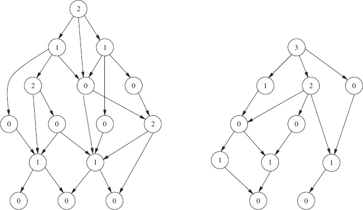
Figure 4.6: Mex numbers. The mex number of a node is the smallest natural number not included among the mex numbers of its successors.
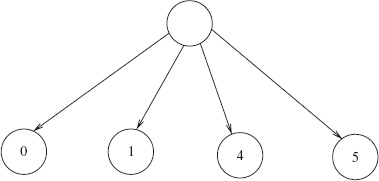
Figure 4.7: Computing mex numbers. The unlabelled node is given the mex number 2.
The algorithm used to calculate mex numbers is an instance of topological search. See Section 16.7.1.
Now, suppose we play this game. Let us suppose the starting position is “Ok”. This is a winning position because the mex number of “O” is different from the mex number of “k”. The latter is larger (3 against 2). So, the winning strategy is to move in the right graph to the node “i”, which has the same mex number as “O”. The opponent is then obliged to move, in either the left or right graph, to a node with mex number different from 2. The first player then repeats the strategy of ensuring that the mex numbers are equal, until eventually the opponent can move no further.
Note that, because of the lack of structure of the individual games, we have to search through all 15 positions of the left game and all 11 positions of the right game, in order to calculate the mex numbers of each position. In total, therefore, we have to search through 26 different positions. But, this is just the sum (in the usual sense of the word) of 15 and 11, and is much less than their product, 165. This is a substantial saving of computational effort. Moreover, the saving grows as the size of the component games increases.
(a) Consider the subtraction-set game where there is one pile of matches from which at most 2, 5 or 6 matches may be removed. Calculate the mex number for each position until you spot a pattern.
(b) Consider a game which is the sum of two games. In the left game, 1 or 2 matches may be removed at each turn. In the right game, 2, 5 or 6 matches may be removed. In the sum game, a move is made by choosing to play in the left game, or choosing to play in the right game.
Table 4.2 shows a number of different positions in this game. A position is given by a pair of numbers: the number of matches in the left pile, and the number of matches in the right pile.
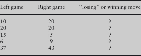
Table 4.2: Fill in entries marked “?”.
For each position, state whether it is a winning or a losing position. For winning positions, give the winning move in the form Xm where “X” is one of “L” (for “left game”) or “R” (for right game), and m is the number of matches to be removed.
Exercise 4.7 A rectangular board is divided into m horizontal rows and n vertical columns, where m and n are both strictly positive integers, making a total of m×n squares. The number of squares is called the area of the board.
A game is played on the board as follows. Each of the two players takes it in turn to cut the board either horizontally or vertically along one of the dividing lines. A cut divides the board into two parts; when a cut has been made a part whose area is at most the area of the other part is discarded. (This means that the part with the smaller area is discarded if the two parts have different areas, and one of the two parts is chosen arbitrarily if the two areas are equal.) For example, if the board has 4×5 squares, a single move reduces it to 2×5, 3×5, 4×3, or 4×4 squares. Also, if the board has 4×4 squares, a single move reduces it to either 2×4 or 3×4 squares. (Boards with 3×4 and 4×3 squares are effectively the same; the orientation of the board is not significant.) The game ends when the board has been reduced to a 1×1 board. At this point, the player whose turn it is to play loses.
This game is a sum game because, at each move, a choice is made between cutting horizontally and cutting vertically. The component games are copies of the same game. This game is as follows. A position in the game is given by a strictly positive integer m. A move in the game is to replace m by a number n such that n < m ≤ 2n; the game ends when m has been reduced to 1, at which point the player whose turn it is to play loses. For example, if the board has 5 columns, the number of columns can be reduced to 3 or 4 because 3 < 5 ≤ 6 and 4 < 5 ≤ 8. No other moves are possible because, for n less than 3, 2n < 5, and for n greater than 4, 5 ≤ n.
The game is easy to win if it is possible to make the board square. This question is about calculating the mex numbers of the component games in order to determine a winning move even when the board cannot be made square.
(a) For the component game, calculate which positions are winning and which positions are losing for the first 15 positions. Make a general conjecture about the winning and losing positions in the component game and prove your conjecture.
Base your proof on the following facts. The end position, position 1, is a losing position. A winning position is a position from which there is a move to a losing position. A losing position is a position from which every move is to a winning position.
(b) For the component game, calculate the mex number of each of the first 15 positions.
Give the results of your calculation in the form of a table with two rows. The first row is a number m and the second row is the mex number of position m. Split the table into four parts. Part i gives the mex numbers of positions 2i thru 2i+1−1 (where i begins at 0) as shown below. (The first three entries have been completed as illustration.)
| Position: | 1 |
| Mex number: | 0 |
| Position: | 2 | 3 |
| Mex number: | 1 | 0 |
| Position: | 4 | 5 | 6 | 7 |
| Mex number: | ? | ? | ? | ? |
| Position: | 8 | 9 | 10 | 11 | 12 | 13 | 14 | 15 |
| Mex number: | ? | ? | ? | ? | ? | ? | ? | ? |
(You should find that the mex number of each of the losing positions (identified in part (a)) is 0. You should also be able to observe a pattern in the way entries are filled in for part i+1 knowing the entries for part i. The pattern is based on whether the position is an even number or an odd number.)
(c) Table 4.3 shows a position in the board game; the first column shows the number of columns and the second column the number of rows. Using your table of mex numbers, or otherwise, fill in “losing” if the position is a losing position. If the position is not a losing position, fill in a winning move either in the form “Cn” or “Rn”, where n is an integer; “C” or “R” indicates whether the move is to reduce the number of columns or the number of rows, and n is the number which it should become.
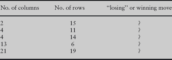
Table 4.3: Fill in entries marked “?”.
4.5 SUMMARY
This chapter has been about determining winning strategies in simple two-person games. The underlying theme of the chapter has been problem specification. We have seen how winning and losing positions are specified. A precise, formal specification enabled us to formulate a brute-force search procedure to determine which positions are which.
Brute-force search is only advisable for small, unstructured problems. The analysis of the “sum” of two games exemplifies the way structure is exploited in problem solving. Again, the focus was on problem specification. By formulating a notion of “symmetry” between the left and right games, we were able to determine a specification of the “mex” function on game positions. The use of mex functions substantially reduces the effort needed to determine winning and losing positions in the sum of two games, compared to a brute-force search.
Game theory is a rich, well-explored area of mathematics, which we have only touched upon in this chapter. It is a theory that is becoming increasingly important in computing science. One reason for this is that problems that beset software design, such as the security of a system, are often modelled as a game, with the user of the software as the adversary. Another reason is that games often provide excellent examples of “computational complexity”; it is easy to formulate games having very simple rules but for which no efficient algorithm implementing the winning strategy is known.
Mex numbers were introduced by Sprague and Grundy to solve the “Nim” problem, and mex numbers are sometimes called “Sprague–Grundy” numbers, after their originators. Nim is a well-known matchstick game involving three piles of matches. Formally, it is the sum of three copies of the same trivial game: given a pile of matches, the players take it in turn to remove any number of matches. (The game is trivial because the obvious winning strategy is to remove all the matches.) We have not developed the theory sufficiently in this chapter to show how Nim, and sums of more than two games, are solved using mex numbers. (What is missing is how to compute mex numbers of positions in the sum of two games.)
4.6 BIBLIOGRAPHIC REMARKS
The two-volume book Winning Ways [BCG82] by Berlekamp, Conway and Guy is essential reading for anyone interested in the theory of combinatorial games. It contains a great wealth of examples and entertaining discussion of strategies for winning.
I do not know the origins of the daisy problem or the coin problem (Section 4.4.2). Both are solved by the simple tactic of copying the opponent’s moves. In the case of the daisy problem, the second player always wins. The first player’s first move destroys the symmetry and, subsequently, the second player restores symmetry by removing petals directly opposite those just removed by the first player. In the case of the coin problem, the first player wins. The first player’s first move is to place a coin at the exact centre of the table. Subsequently the first player copies the second player’s move by placing a coin diagonally opposite the one just placed on the table by the second player. Again, every move made by the second player destroys symmetry and the first player restores the symmetry. The coins may be of any shape (circular, rectangular or even misshapen) provided two conditions are met. Firstly, the coin used for the very first move must be symmetrical about a centre point and should not have a hole in the centre that can be filled by another coin. Secondly, for all other moves, the first player should always be able to choose a coin that is identical to the one just used by the second player.
The 31st December game (Exercise 4.1) is adapted from [DW00]. Exercise 4.7 was suggested to me by Atheer Aheer. (I do not know its origin.)
1Recall that n mod 3 denotes the remainder after dividing n by 3.
2You may wish to review Section 3.6 on the formulation and use of conditional statements.
3The word “falsify” can be found in an English dictionary, but not “truthify”. “Falsify” means to make something false; we use “truthify” for the opposite: making something true. It is so common in algorithmic problem solving that it deserves to be in the dictionary. “Truthify” was coined by David Gries.