Serious Cryptography

12
ELLIPTIC CURVES

The introduction of elliptic curve cryptography (ECC) in 1985 revolutionized the way we do public-key cryptography. ECC is more powerful and efficient than alternatives like RSA and classical Diffie–Hellman (ECC with a 256-bit key is stronger than RSA with a 4096-bit key), but it’s also more complex.

Like RSA, ECC multiplies large numbers, but unlike RSA it does so in order to combine points on a mathematical curve, called an elliptic curve (which has nothing to do with an ellipse, by the way). To complicate matters, there are many different types of elliptic curves—simple and sophisticated ones, efficient and inefficient ones, and secure and insecure ones.

Although first introduced in 1985, ECC wasn’t adopted by standardization bodies until the early 2000s, and it wasn’t seen in major toolkits until much later: OpenSSL added ECC in 2005, and the OpenSSH secure connectivity tool waited until 2011. But modern systems have few reasons not to use ECC, and you’ll find it used in Bitcoin and many security components in Apple devices. Indeed, elliptic curves allow you to perform common public-key cryptography operations such as encryption, signature, and key agreement faster than their classical counterparts. Most cryptographic applications that rely on the discrete logarithm problem (DLP) will also work when based on its elliptic curve counterpart, ECDLP, with one notable exception: the Secure Remote Password (SRP) protocol.

This chapter focuses on applications of ECC and discusses why you would use ECC rather than RSA or classical Diffie–Hellman, as well as how to choose the right elliptic curve for your application.

What Is an Elliptic Curve?

An elliptic curve is a curve on a plane—a group of points with x and y coordinates. A curve’s equation defines all the points that belong to that curve. For example, the curve y = 3 is a horizontal line with the vertical coordinate 3, curves of the form y = ax + b with fixed numbers a and b are straight lines, x² + y² = 1 is a circle of radius 1 centered on the origin, and so on. Whatever the type of curve, the points on a curve are all (x, y) pairs that satisfy the curve’s equation.

An elliptic curve as used in cryptography is typically a curve whose equation is of the form y² = x³ + ax + b (known as the Weierstrass form), where the constants a and b define the shape of the curve. For example, Figure 12-1 shows the elliptic curve that satisfies the equation y² = x³ – 4x.

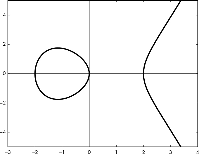
Figure 12-1: An elliptic curve with the equation y² = x³ – 4x, shown over the real numbers

NOTE

In this chapter, I focus on the simplest, most common type of elliptic curves—namely, those with an equation that looks like y² = x³ + ax + b—but there are types of elliptic curves with equations in other forms. For example, Edwards curves are elliptic curves whose equation is of the form x² + y² = 1 + dx²y². Edwards curves are sometimes used in cryptography (for example, in the Ed25519 scheme).

Figure 12-1 shows all the points that make up the curve for x between –3 and 4, be they points on the left side of the curve, which looks like a circle, or on the right side, which looks like a parabola. All these points have (x, y) coordinates that satisfy the curve’s equation y² = x³ – 4x. For example, when x = 0, then y² = x³ – 4x = 0³ – 4 × 0 = 0; hence, y = 0 is a solution, and the point (0, 0) belongs to the curve. Likewise, if x = 2, the solution to the equation is y = 0, meaning that the point (2, 0) belongs to the curve.

It is crucial to distinguish points that belong to the curve from other points, because when using elliptic curves for cryptography, we’ll be working with points from the curve, and points off the curve often present a security risk. However, note that the curve’s equation doesn’t always admit solutions, at least not in the natural number plane. For example, to find points with the horizontal coordinate x = 1, we solve y² = x³ – 4x for y² with x³ – 4x = 1³ – 4 × 1, giving a result of –3. But y² = –3 doesn’t have a solution because there is no number for which y² = –3. (There is a solution in the complex numbers, but elliptic curve cryptography will only deal with natural numbers—more precisely, integers modulo a prime.) Because there is no solution to the curve’s equation for x = 1, the curve has no point at that position on the x-axis, as you can see in Figure 12-1.

What if we try to solve for x = –1? In this case, we get the equation y² = –1 + 4 = 3, which has two solutions (y = √3 and y = –√3), the square root of three and its negative value. Squaring a number always gives a positive number, so y² = (–y)² for any real number y, and as you can see, the curve in Figure 12-1 is symmetric with respect to the x-axis for all points that solve its equation (as are all elliptic curves of the form y² = x³ + ax + b).

Elliptic Curves over Integers

Now here’s a bit of a twist: the curves used in elliptic curve cryptography actually don’t look like the curve shown in Figure 12-1. They look instead like Figure 12-2, which is a cloud of points rather than a curve. What’s going on here?

Figures 12-1 and 12-2 are actually based on the same curve equation, y² = x³ – 4x, but they show the curve’s points with respect to different sets of numbers: Figure 12-1 shows the curve’s points over the set of real numbers, which includes negative numbers, decimals, and so on. For example, as a continuous curve, it shows the points at x = 2.0, x = 2.1, x = 2.00002, and so on. Figure 12-2, on the other hand, shows only integers that satisfy this equation, which excludes decimal numbers. Specifically, Figure 12-2 shows the curve y² = x³ – 4x with respect to the integers modulo 191: 0, 1, 2, 3, up to 190. This set of numbers is denoted Z₁₉₁. (There’s nothing special with 191 here, except that it’s a prime number. I picked a small number to avoid having too many points on the graph.) The points shown on Figure 12-2 therefore all have x and y coordinates that are integers modulo 191 and that satisfy the equation y² = x³ – 4x. For example, for x = 2, we have y² = 0, for which y = 0 is a valid solution. This tells us that the point (2, 0) belongs to the curve.

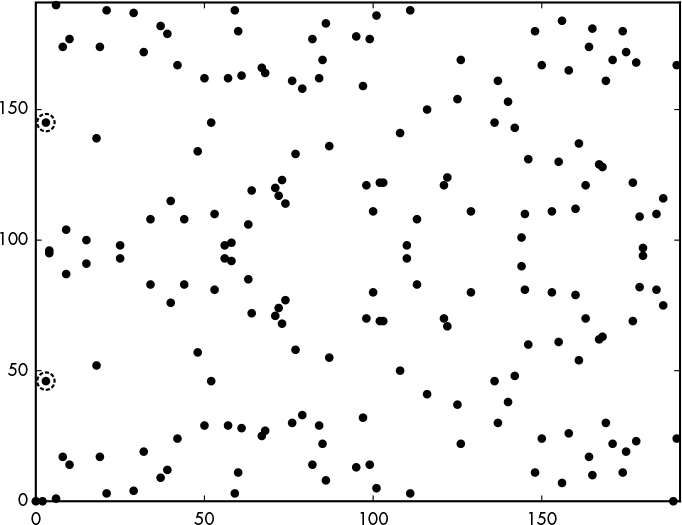
Figure 12-2: The elliptic curve with the equation y² = x³ – 4x over Z₁₉₁, the set of integers modulo 191

What if x = 3? We get the equation y² = 27 – 12 = 15, which admits two solutions to y² = 15 (namely, 46 and 145), because 46² mod 191 = 15 and 145² mod 191 = 15 both equal 15 in Z₁₉₁. Thus, the points (3, 46) and (3, 145) belong to the curve and appear as shown in Figure 12-2 (the two points highlighted at the left).

NOTE

Figure 12-2 considers points from the set denoted Z₁₉₁ = {0, 1, 2, . . . , 190}, which includes zero. This differs from the groups denoted Z_p^* (with a star superscript) that we discussed in the context of RSA and Diffie–Hellman. The reason for this difference is that we’ll both multiply and add numbers, and we therefore need to ensure that the set of numbers includes addition’s identity element (namely 0, such that x + 0 = x for every x in Z₁₉₁). Also, every number x has an inverse with respect to addition, denoted –x, such that x + (–x) = 0. For example, the inverse of 100 in Z₁₉₁ is 91, because 100 + 91 mod 191 = 0. Such a set of numbers, where addition and multiplication are possible and where each element x admits an inverse with respect to addition (denoted –x) as well as an inverse with respect to multiplication (denoted 1 / x), is called a field. When a field has a finite number of elements, as in Z₁₉₁ and as with all fields used for elliptic curve cryptography, it is called a finite field.

Adding and Multiplying Points

We’ve seen that the points on an elliptic curve are all coordinates (x, y) that satisfy the curve’s equation, y² = x³ + ax + b. In this section, we look at how to add elliptic curve points, a rule called the addition law.

Adding Two Points

Say that we want to add two points on the elliptic curve, P and Q, to give a new point, R, that is the sum of these two points. The simplest way to understand point addition is to determine the position of R = P + Q on the curve relative to P and Q based on a geometric rule: draw the line that connects P and Q, find the other point of the curve that intersects with this line, and Q is the reflection of this point with respect to the x-axis. For example, in Figure 12-3, the line connecting P and Q intersects the curve at a third point between P and Q, and the point P + Q is the point at the same x coordinate but the inverse y coordinate.

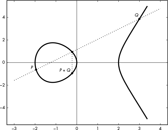
Figure 12-3: A general case of the geometric rule for adding points over an elliptic curve

This geometric rule is simple, but it won’t directly give you the coordinates of the point R. We compute the coordinates (x_R, y_R) of R using the coordinates (x_p , y_p) of P and the coordinates (x_Q, y_Q) of Q using the formulas x_R = m² – x_p – x_Q and y_R = m(x_p – x_R) – y_p , where the value m = (y_Q – y_p) / (x_Q – x_p) is the slope of the line connecting P and Q.

Unfortunately, these formulas and the line-drawing trick shown in Figure 12-3 don’t always work. If, for example, P = Q, you can’t draw a line between two points (there’s only one), and if P = –P, the line doesn’t cross the curve again, so there is no point on the curve to mirror. We’ll explore these in the next section.

Adding a Point and Its Negative

The negative of a point P = (x_P , y_P) is the point –P = (x_P , –y_P), which is the point mirrored around the x-axis. For any P, we say that P + (–P) = O, where O is called the point at infinity. And as you can see in Figure 12-4, the line between P and –P runs to infinity and never intersects the curve. (The point at infinity is a virtual point that belongs to any elliptic curve; it is to elliptic curves what zero is to integers.)

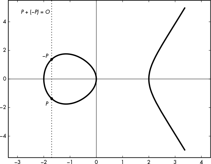
Figure 12-4: The geometric rule for adding points on an elliptic curve with the operation P + (–P) = O when the line between the points never intersects the curve

Doubling a Point

When P = Q (that is, P and Q are at the same position), adding P and Q is equivalent to computing P + P, also denoted 2P. This addition operation is therefore called a doubling.

However, to find the coordinates of the result R = 2P, we can’t use the geometric rule from the previous section, because we can’t draw a line between P and itself. Instead, we draw the line tangent to the curve at P, and 2P is the negation of the point where this line intersects the curve, as shown on Figure 12-5.

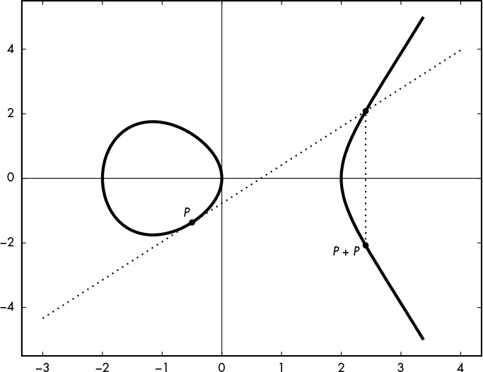
Figure 12-5: The geometric rule for adding points over an elliptic curve using the doubling operation P + P

The formula for determining the coordinates (x_R, y_R) of R = P + P is slightly different from the formula we would use for a distinct P and Q. Again, the basic formula is x_R = m² – x_p – x_Q and y_R = m(x_p – x_R) – y_p, but the value of m is different; it becomes (3x_p² + a) / 2y_p, where a is the curve’s parameter, as in y² = x³ + ax + b.

Multiplication

In order to multiply points on elliptic curves by a given number k, where k is an integer, we determine the point kP by adding P to itself k – 1 times. In other words, 2P = P + P, 3P = P + P + P, and so on. To obtain the x and y coordinates of kP, repeatedly add P to itself and apply the preceding addition law.

To compute kP efficiently, however, the naive technique of adding P by applying the addition law k – 1 times is far from optimal. For example, if k is large (of the order of, say, 2²⁵⁶) as it occurs in elliptic curve–based crypto schemes, then computing k – 1 additions is downright infeasible.

But there’s a trick: you can gain an exponential speed-up by adapting the technique discussed in “Fast Exponentiation Algorithm: Square-and-Multiply” on page 192 to compute x^e mod n. For example, to compute 8P in three additions instead of seven using the naive method, you would first compute P₂ = P + P, then P₄ = P₂ + P₂, and finally P₄ + P₄ = 8P.

Elliptic Curve Groups

Because points can be added together, the set of points on an elliptic curve forms a group. According to the definition of a group (see “What Is a Group?” on page 174), if the points P and Q belong to a given curve, then P + Q also belongs to the curve.

Furthermore, because addition is associative, we have (P + Q) + R = P + (Q + R) for any points P, Q, and R. In a group of elliptic curve points, the identity element is called the point at infinity, and denoted O, such that P + O = P for any P. Every point P = (x_P , y_P) has an inverse, –P = (x_P , –y_P), such that P + (–P) = O.

In practice, most elliptic curve–based cryptosystems work with x and y coordinates that are numbers modulo a prime number, p (in other words, numbers in the finite field Z_p). Just as the security of RSA depends on the size of the numbers used, the security of an elliptic curve–based cryptosystem depends on the number of points on the curve. But how do we know the number of points on an elliptic curve, or its cardinality? Well, it depends on the curve and the value of p.

One rule of thumb is that there are approximately p points on the curve, but you can compute the exact number of points with Schoof’s algorithm, which counts points on elliptic curves over finite fields. You’ll find this algorithm built in to SageMath. For example, Listing 12-1 shows how to use this algorithm to count the number of points on the curve y² = x³ – 4x over Z₁₉₁ shown in Figure 12-1.

sage: Z = Zmod(191)
sage: E = EllipticCurve(Z, (-4,0))
sage: E.cardinality()
192

Listing 12-1: Computing the cardinality, or number of points on a curve

In Listing 12-1, we’ve first defined the variable Z as the set over integers modulo 191; then we defined the variable E as the elliptic curve over Z with the coefficients –4 and 0. Finally, we computed the number of points on the curve, also known as its cardinality, group order, or just order. Note that this count includes the point at infinity O.

The ECDLP Problem

Chapter 9 introduced the DLP: that of finding the number y given some base number g, where x = g ^y mod p for some large prime number p. Cryptography with elliptic curves has a similar problem: the problem of finding the number k given a base point P where the point Q = kP. This is called the elliptic curve discrete logarithm problem, or ECDLP. (Instead of numbers, the elliptic curve’s problems operate on points, and multiplication is used instead of exponentiation.)

All elliptic curve cryptography is built on the ECDLP problem, which, like DLP, is believed to be hard and has withstood cryptanalysis since its introduction into cryptography in 1985. One important difference between ECDLP and the classical DLP is that ECDLP allows you to work with smaller numbers and still enjoy a similar level of security.

Generally, when p is n bits, you’ll get a security level of about n / 2 bits. For example, an elliptic curve taken over numbers modulo p, with a 256-bit p, will give a security level of about 128 bits. For the sake of comparison, to achieve a similar security level with DLP or RSA, you would need to use numbers of several thousands of bits. The smaller numbers used for ECC arithmetic are one reason why it’s often faster than RSA or classical Diffie–Hellman.

One way of solving ECDLP is to find a collision between two outputs, c₁P + d₁Q and c₂P + d₂Q. The points P and Q in these equations are such that Q = kP for some unknown k, and c₁, d₁, c₂, and d₂ are the numbers you will need in order to find k.

As with the hash function discussed in Chapter 6, a collision occurs when two different inputs produce the same output. Therefore, in order to solve ECDLP, we need to find points where the following is true:

c₁P + d₁Q = c₂P + d₂Q

In order to find these points, we replace Q with the value kP, and we have the following:

c₁P + d₁kP = (c₁ + d₁k)P = c₂P + d₂kP = (c₂ + d₂k)P

This tells us that (c₁ + d₁k) equals (c₂ + d₂k) when taken modulo the number of points on the curve, which is not a secret.

From this, we can deduce the following:

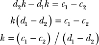
And we’ve found k, the solution to ECDLP.

Of course, that’s only the big picture—the details are more complex and interesting. In practice, elliptic curves extend over numbers of at least 256 bits, which makes attacking elliptic curve cryptography by finding a collision impractical because doing so takes up to 2¹²⁸ operations (the cost of finding a collision over 256-bit numbers, as you learned in Chapter 6).

Diffie–Hellman Key Agreement over Elliptic Curves

Recall from Chapter 11 that in the classical Diffie–Hellman (DH) key agreement protocol, two parties establish a shared secret by exchanging non-secret values. Given some fixed number g, Alice picks a secret random number a, computes A = g^a, sends A to Bob, and Bob picks a secret random b and sends B = g^b to Alice. Both then combine their secret key with the other’s public key to produce the same A^b = B^a = g^ab.

The elliptic curve version of DH is identical to that of classical DH but with different notations. In the case of ECC, for some fixed point G, Alice picks a secret random number d^A, computes P^A = d^AG (the point G multiplied by d_A), and sends P_A to Bob. Bob picks a secret random d_B, computes the point P_B = d_BG, and sends it to Alice. Then both compute the same shared secret, d^AP^B = d^BP^A = d^Ad^BG. This method is called elliptic curve Diffie–Hellman, or ECDH.

ECDH is to the ECDLP problem what DH is to DLP: it’s secure as long as ECDLP is hard. DH protocols that rely on DLP can therefore be adapted to work with elliptic curves and rely on ECDLP as a hardness assumption. For example, authenticated DH and Menezes–Qu–Vanstone (MQV) will also be secure when used with elliptic curves. (In fact, MQV was first defined as working over elliptic curves.)

Signing with Elliptic Curves

The standard algorithm used for signing with ECC is ECDSA, which stands for elliptic curve digital signature algorithm. This algorithm has replaced RSA signatures and classical DSA signatures in many applications. It is, for example, the only signature algorithm used in Bitcoin and is supported by many TLS and SSH implementations.

As with all signature schemes, ECDSA consists of a signature generation algorithm that the signer uses to create a signature using their private key and a verification algorithm that a verifier uses to check a signature’s correctness given the signer’s public key. The signer holds a number, d, as a private key, and verifiers hold the public key, P = dG. Both know in advance what elliptic curve to use, its order (n, the number of points in the curve), as well as the coordinates of a base point, G.

ECDSA Signature Generation

In order to sign a message, the signer first hashes the message with a cryptographic hash function such as SHA-256 or BLAKE2 to generate a hash value, h, that is interpreted as a number between 0 and n – 1. Next, the signer picks a random number, k, between 1 and n – 1 and computes kG, a point with the coordinates (x, y). The signer now sets r = x mod n and computes s = (h + rd) / k mod n, and then uses these values as the signature (r, s).

The length of the signature will depend on the coordinate lengths being used. For example, when you’re working with a curve where coordinates are 256-bit numbers, r and s would both be 256 bits long, yielding a 512-bit-long signature.

ECDSA Signature Verification

The ECDSA verification algorithm uses a signer’s public key to verify the validity of a signature.

In order to verify an ECDSA signature (r, s) and a message’s hash, h, the verifier first computes w = 1 / s, the inverse of s in the signature, which is equal to k / (h + rd) mod n, since s is defined as s = (h + rd) / k. Next, the verifier multiplies w with h to find u according to the following formula:

wh = hk (h + rd) = u

The verifier then multiplies w with r to find v:

wr = rk(h + rd) = v

Given u and v, the verifier computes the point Q according to the following formula:

Q = uG + vP

Here, P is the signer’s public key, which is equal to dG, and the verifier only accepts the signature if the x coordinate of Q is equal to the value r from the signature.

This process works because, as a last step, we compute the point Q by substituting the public key P with its actual value dG:

uG + vdG = (u + vd)G

When we replace u and v with their actual values, we obtain the following:

u + vd = hk (h + rd) + drk / (h + rd) = (hk + drk) / (h + rd) = k (h + dr) / (h + rd) = k

This tells us that (u + vd) is equal to the value k, chosen during signature generation, and that uG + vdG is equal to the point kG. In other words, the verification algorithm succeeds in computing point kG, the same point computed during signature generation. Validation is complete once a verifier confirms that kG’s x coordinate is equal to the r received; otherwise, the signature is rejected as invalid.

ECDSA vs. RSA Signatures

Elliptic curve cryptography is often viewed as an alternative to RSA for public-key cryptography, but ECC and RSA don’t have much in common. RSA is only used for encryption and signatures, whereas ECC is a family of algorithms that can be used to perform encryption, generate signatures, perform key agreement, and offer advanced cryptographic functionalities such as identity-based encryption (a kind of encryption that uses encryption keys derived from a personal identifier, such as an email address).

When comparing RSA and ECC’s signature algorithms, recall that in RSA signatures, the signer uses their private key d to compute a signature as y = x^d mod n, where x is the data to be signed and y is the signature. Verification uses the public key e to confirm that y^e mod n equals x—a process that’s clearly simpler than that of ECDSA.

RSA’s verification process is often faster than ECC’s signature generation because it uses a small public key e. But ECC has two major advantages over RSA: shorter signatures and signing speed. Because ECC works with shorter numbers, it produces shorter signatures than RSA (hundreds of bits long, not thousands of bits), which is an obvious benefit if you have to store or transmit numerous signatures. Signing with ECDSA is also much faster than signing with RSA (though signature verification is about as fast) because ECDSA works with much smaller numbers than RSA does for a similar security level. For example, Listing 12-2 shows that ECDSA is about 150 times faster at signing and a little faster at verifying. Note that ECDSA signatures are also shorter than RSA signatures because they’re 512 bits (two elements of 256 bits each) rather than 4096 bits.

$ openssl speed ecdsap256 rsa4096
                              sign     verify     sign/s     verify/s
rsa 4096 bits            0.007267s  0.000116s      137.6       8648.0
                              sign     verify     sign/s     verify/s
256 bit ecdsa (nistp256)   0.0000s    0.0001s    21074.6       9675.7

Listing 12-2: Comparing the speed of 4096-bit RSA signatures with 256-bit ECDSA signatures

It’s fair to compare the performance of these differently sized signatures because they provide a similar security level. However, in practice, many systems use RSA signatures with 2048 bits, which is orders of magnitude less secure than 256-bit ECDSA. Thanks to its smaller modulus size, 2048-bit RSA is faster than 256-bit ECDSA at verifying, yet still slower at signing, as shown in Listing 12-3.

$ openssl speed rsa2048
sign verify sign/s verify/s
rsa 2048 bits 0.000696s 0.000032s 1436.1 30967.1

Listing 12-3: The speed of 2048-bit RSA signatures

The upshot is that you should prefer ECDSA to RSA except when signature verification is critical and you don’t care about signing speed, as in a sign-once, verify-many situation (for example, when a Windows executable application is signed once and then verified by all the systems executing it).

Encrypting with Elliptic Curves

Although elliptic curves are more commonly used for signing, you can still encrypt with them. But you’ll rarely see people do so in practice due to restrictions in the size of the plaintext that can be encrypted: you can fit only about 100 bits of plaintext, as compared to almost 4000 in RSA with the same security level.

One simple way to encrypt with elliptic curves is to use the integrated encryption scheme (IES), a hybrid asymmetric–symmetric key encryption algorithm based on the Diffie–Hellman key exchange. Essentially, IES encrypts a message by generating a Diffie–Hellman key pair, combining the private key with the recipient’s own public key, deriving a symmetric key from the shared secret obtained, and then using an authenticated cipher to encrypt the message.

When used with elliptic curves, IES relies on ECDLP’s hardness and is called elliptic-curve integrated encryption scheme (ECIES). Given a recipient’s public key, P, ECIES encrypts a message, M, as follows:

Pick a random number, d, and compute the point Q = dG, where the base point G is a fixed parameter. Here, (d, Q) acts as an ephemeral key pair, used only for encrypting M.
Compute an ECDH shared secret by computing S = dP.
Use a key derivation scheme (KDF) to derive a symmetric key, K, from S.
Encrypt M using K and a symmetric authenticated cipher, obtaining a ciphertext, C, and an authentication tag, T.

The ECIES ciphertext then consists of the ephemeral public key Q followed by C and T. Decryption is straightforward: the recipient computes S by multiplying R with their private exponent to obtain S, and then derives the key K and decrypts C and verifies T.

Choosing a Curve

Criteria used to assess the safety of an elliptic curve include the order of the group used (that is, its number of points), its addition formulas, and its origins.

There are several types of elliptic curves, but not all are equally good for cryptographic purposes. When making your selection, be sure to choose coefficients a and b in the curve’s equation y² = x³ + ax + b carefully; otherwise, you may end up with an insecure curve. In practice, you’ll use some de facto standard curve for encryption, but knowing what makes a safe curve will help you choose among the several available ones and better understand any associated risks. Here are some points to keep in mind:

The order of the group should not be a product of small numbers; otherwise solving ECDLP becomes much easier.
In “Adding and Multiplying Points” on page 221, you learned that adding points P + Q required a specific addition formula when Q = P. Unfortunately, treating this case differently from the general one may leak critical information if an attacker is able to distinguish doublings from additions between distinct points. Some curves are secure because they use a single formula for all point addition. (When a curve does not require a specific formula for doublings, we say that it admits a unified addition law.)
If the creators of a curve don’t explain the origin of a and b, they may be suspected of foul play because you can’t know whether they may have chosen weaker values that enable some yet-unknown attack on the cryptosystem.

Let’s review some of the most commonly used curves, especially ones used for signatures or Diffie–Hellman key agreement.

NOTE

You’ll find more criteria and more details about curves on the dedicated website https://safecurves.cr.yp.to/.

NIST Curves

In 2000, the NIST curves were standardized by the US NIST in the FIPS 186 document under “Recommended Elliptic Curves for Federal Government Use.” Five NIST curves work modulo a prime number (as discussed in “Elliptic Curves over Integers” on page 219), called prime curves. Ten other NIST curves work with binary polynomials, which are mathematical objects that make implementation in hardware more efficient. (We won’t cover binary polynomials in further detail because they’re seldom used with elliptic curves.)

The most common NIST curves are the prime curves. Of these, one of the most common is P-256, a curve that works over numbers modulo the 256-bit number p = 2²⁵⁶ – 2²²⁴ + 2¹⁹² + 2⁹⁶ – 1. The equation for P-256 is y² = x³ – 3x + b, where b is a 256-bit number. NIST also provides prime curves of 192 bits, 224 bits, 384 bits, and 521 bits.

NIST curves are sometimes criticized because only the NSA, creator of the curves, knows the origin of the b coefficient in their equations. The only explanation we’ve been given is that b results from hashing a random-looking constant with SHA-1. For example, P-256’s b parameter comes from the following constant: c49d3608 86e70493 6a6678e1 139d26b7 819f7e90.

No one knows why the NSA picked this particular constant, but most experts don’t believe the curve’s origin hides any weakness.

Curve25519

Daniel J. Bernstein brought Curve25519 (pronounced curve-twenty-five-five-nineteen) to the world in 2006. Motivated by performance, he designed Curve25519 to be faster and use shorter keys than the standard curves. But Curve25519 also brings security benefits, because unlike the NIST curves it has no suspicious constants and can use the same unified formula for adding distinct points or for doubling a point.

The form of Curve25519’s equation, y² = x³ + 486662x² + x, is slightly different from that of the other equations you’ve seen in this chapter, but it still belongs to the elliptic curve family. The unusual form of this equation allows for specific implementation techniques that make Curve25519 fast in software.

Curve25519 works with numbers modulo the prime number 2²⁵⁵ – 19, a 256-bit prime number that is as close as possible to 2²⁵⁵. The b coefficient 486662 is the smallest integer that satisfies the security criteria set by Bernstein. Taken together, these features make Curve25519 more trustworthy than NIST curves and their fishy coefficients.

Curve25519 is used everywhere: in Google Chrome, Apple systems, OpenSSH, and many other systems. However, because Curve25519 isn’t a NIST standard, some applications stick to NIST curves.

NOTE

To learn all the details and rationale behind Curve25519, view the 2016 presentation “The first 10 years of Curve25519” by Daniel J. Bernstein, available at http://cr.yp.to/talks.html#2016.03.09/.

Other Curves

As I write this, most cryptographic applications use NIST curves or Curve25519, but there are other legacy standards in use, and newer curves are being promoted and pushed within standardization committees. Some of the old national standards include France’s ANSSI curves and Germany’s Brainpool curves: two families that don’t support complete addition formulas and that use constants of unknown origins.

Some newer curves are more efficient than the older ones and are clear of any suspicion; they offer different security levels and various efficiency optimizations. Examples include Curve41417, a variant of Curve25519, which works with larger numbers and offers a higher level of security (approximately 200 bits); Ed448-Goldilocks, a 448-bit curve first proposed in 2014 and considered to be an internet standard; as well as six curves proposed by Aranha et al. in “A note on high-security general-purpose elliptic curves” (see http://eprint.iacr.org/2013/647/), though these curves are rarely used. The details specific to all these curves are beyond the scope of this book.

How Things Can Go Wrong

Elliptic curves have their downsides due to their complexity and large attack surface. Their use of more parameters than classical Diffie–Hellman brings with it a greater attack surface with more opportunities for mistakes and abuse—and possible software bugs that might affect their implementation. Elliptic curve software may also be vulnerable to side-channel attacks due to the large numbers used in their arithmetic. If the speed of calculations depends on inputs, attackers may be able to obtain information about the formulas being used to encrypt.

In the following sections, I discuss two examples of vulnerabilities that can occur with elliptic curves, even when the implementation is safe. These are protocol vulnerabilities rather than implementation vulnerabilities.

ECDSA with Bad Randomness

ECDSA signing is randomized, as it involves a secret random number k when setting s = (h + rd) / k mod n. However, if the same k is reused to sign a second message, an attacker could combine the resulting two values, s₁ = (h₁ + rd) / k and s₂ = (h₂ + rd) / k, to get s₁ – s₂ = (h₁ – h₂) / k and then k = (h₁ – h₂) / (s₁ – s₂). When k is known, the private key d is easily recovered by computing the following:

(ks₁ − h₁) / r = ((h₁ + rd) − h₁) / r = rd / r = d

Unlike RSA signatures, which won’t allow the key to be recovered if a weak pseudorandom number generator (PRNG) is used, the use of non-random numbers can lead to ECDSA’s k being recoverable, as happened with the attack on the PlayStation 3 game console in 2010, presented by the fail0verflow team at the 27th Chaos Communication Congress in Berlin, Germany.

Breaking ECDH Using Another Curve

ECDH can be elegantly broken if you fail to validate input points. The primary reason is that the formulas that give the coordinates for the sum of points P + Q never involve the b coefficient of the curve; instead, they rely only on the coordinates of P and Q and the a coefficient (when doubling a point). The unfortunate consequence of this is that when adding two points, you can never be sure that you’re working on the right curve because you may actually be adding points on a different curve with a different b coefficient. That means you can break ECDH as described in the following scenario, called the invalid curve attack.

Say that Alice and Bob are running ECDH and have agreed on a curve and a base point, G. Bob sends his public key d_BG to Alice. Alice, instead of sending a public key d_AG on the agreed upon curve, sends a point on a different curve, either intentionally or accidentally. Unfortunately, this new curve is weak and allows Alice to choose a point P for which solving ECDLP is easy. She chooses a point of low order, for which there is a relatively small k such that kP = O.

Now Bob, believing that he has a legitimate public key, computes what he thinks is the shared secret d_BP, hashes it, and uses the resulting key to encrypt data sent to Alice. The problem is that when Bob computes d_BP, he is unknowingly computing on the weaker curve. As a result, because P was chosen to belong to a small subgroup within the larger group of points, the result d_BP will also belong to that small subgroup, allowing an attacker to determine the shared secret d_BP efficiently if they know the order of P.

One way to prevent this is to make sure that points P and Q belong to the right curve by ensuring that their coordinates satisfy the curve’s equation. Doing so would prevent this attack by making sure that you’re only able to work on the secure curve.

Such an invalid curve attack was found in 2015 on certain implementations of the TLS protocol, which uses ECDH to negotiate session keys. (For details, see the paper “Practical Invalid Curve Attacks on TLS-ECDH” by Jager, Schwenk, and Somorovsky.)

Table of Contents for
Serious Cryptography