Table of Contents for

Serious Cryptography

9
HARD PROBLEMS

Hard computational problems are the cornerstone of modern cryptography. They’re problems that are simple to describe yet practically impossible to solve. These are problems for which even the best algorithm wouldn’t find a solution before the sun burns out.

In the 1970s, the rigorous study of hard problems gave rise to a new field of science called computational complexity theory, which would dramatically impact cryptography and many other fields, including economics, physics, and biology. In this chapter, I’ll give you the conceptual tools from complexity theory necessary to understand the foundations of cryptographic security, and I’ll introduce the hard problems behind public-key schemes such as RSA encryption and Diffie–Hellman key agreement. We’ll touch on some deep concepts, but I’ll minimize the technical details and only scratch the surface. Still, I hope you’ll see the beauty in the way cryptography leverages computational complexity theory to maximize security.

Computational Hardness

A computational problem is a question that can be answered by doing enough computation, for example, “Is 2017 a prime number?” or “How many i letters are there in incomprehensibilities?” Computational hardness is the property of computational problems for which there is no algorithm that will run in a reasonable amount of time. Such problems are also called intractable problems and are often practically impossible to solve.

Surprisingly, computational hardness is independent of the type of computing device used, be it a general-purpose CPU, an integrated circuit, or a mechanical Turing machine. Indeed, one of the first findings of computational complexity theory is that all computing models are equivalent. If a problem can be solved efficiently with one computing device, it can be solved efficiently on any other device by porting the algorithm to the other device’s language—an exception is quantum computers, but these do not exist (yet). The upshot is that we won’t need to specify the underlying computing device or hardware when discussing computational hardness; instead, we’ll just discuss algorithms.

To evaluate hardness, we’ll first find a way to measure the complexity of an algorithm, or its running time. We’ll then categorize running times as hard or easy.

Measuring Running Time

Most developers are familiar with computational complexity, or the approximate number of operations done by an algorithm as a function of its input size. The size is counted in bits or in the number of elements taken as input. For example, take the algorithm shown in Listing 9-1, written in pseudocode. It searches for a value, x, within an array of n elements and then returns its index position.

search(x, array, n):
    for i from 1 to n {
        if (array[i] == x) {
            return i;
        }
    }
    return 0;
}

Listing 9-1: A simple search algorithm, written in pseudocode, of complexity linear with respect to the array length n. The algorithm returns the index where the value x is found in [1, n], or 0 if x isn’t found in the array.

In this algorithm, we use a for loop to find a specific value, x, by iterating through an array. On each iteration, we assign the variable i a number starting with 1. Then we check whether the value of position i in array is equal to the value of x. If it is, we return the position i. Otherwise, we increment i and try the next position until we reach n, the length of the array, at which point we return 0.

For this kind of algorithm, we count complexity as the number of iterations of the for loop: 1 in the best case (if x is equal to array[1]), n in the worst case (if x is equal to array[n] or if x is not in found in array), and n/2 on average if x is randomly distributed in one of the n cells of the array. With an array 10 times as large, the algorithm will be 10 times as slow. Complexity is therefore proportional to n, or “linear” in n. A complexity linear in n is considered fast, as opposed to complexities exponential in n. Although processing larger input values will be slower, it will make a difference of at most just seconds for most practical uses.

But many useful algorithms are slower than that and have a complexity higher than linear. The textbook example is sorting algorithms: given a list of n values in a random order, you’ll need on average n × log n basic operations to sort the list, which is sometimes called linearithmic complexity. Since n × log n grows faster than n, sorting speed will slow down faster than proportionally to n. Yet such sorting algorithms will remain in the realm of practical computation, or computation that can be carried out in a reasonable amount of time.

At some point, we’ll hit the ceiling of what’s feasible even for relatively small input lengths. Take the simplest example from cryptanalysis: the brute-force search for a secret key. Recall from Chapter 1 that given a plaintext P and a ciphertext C = E(K, P), it takes at most 2ⁿ attempts to recover an n-bit symmetric key because there are 2ⁿ possible keys—an example of a complexity that grows exponentially. For complexity theorists, exponential complexity means a problem that is practically impossible to solve, because as n grows, the effort very rapidly becomes infeasible.

You may object that we’re comparing oranges and apples here: in the search() function in Listing 9-1, we counted the number of if (array[i] == x) operations, whereas key recovery counts the number of encryptions, each thousands of times slower than a single == comparison. This inconsistency can make a difference if you compare two algorithms with very similar complexities, but most of the time it won’t matter because the number of operations will have a greater impact than the cost of an individual operation. Also, complexity estimates ignore constant factors: when we say that an algorithm takes time in the order of n³ operations (which is quadratic complexity), it may actually take 41 × n³ operations, or 12345 × n³ operations—but again, as n grows, the constant factors lose significance to the point that we can ignore them. Complexity analysis is about theoretical hardness as a function of the input size; it doesn’t care about the exact number of CPU cycles it will take on your computer.

You’ll often find the O() notation (“big O”) used to express complexities. For example, O(n³) means that complexity grows no faster than n³, ignoring potential constant factors. O() denotes the upper bound of an algorithm’s complexity. The notation O(1) means that an algorithm runs in constant time—that is, the running time doesn’t depend on the input length! For example, the algorithm that determines an integer’s parity by looking at its least significant bit (LSB) and returning “even” if it’s zero and “odd” otherwise will do the same thing at the same cost whatever the integer’s length.

To see the difference between linear, quadratic, and exponential time complexities, look at how complexity grows for O(n) (linear) versus O(n²) (quadratic) versus O(2ⁿ) (exponential) in Figure 9-1.

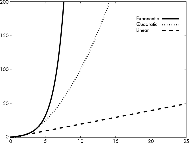
Figure 9-1: Growth of exponential, quadratic, and linear complexities, from the fastest to the slowest growing

Exponential complexity means the problem is practically impossible to solve, and linear complexity means the solution is feasible, whereas quadratic complexity is somewhere between the two.

Polynomial vs. Superpolynomial Time

The O(n²) complexity discussed in the last section (the middle curve in Figure 9-1) is a special case of the broader class of polynomial complexities, or O(n^k), where k is some fixed number such as 3, 2.373, 7/10, or the square root of 17. Polynomial-time algorithms are eminently important in complexity theory and in crypto because they’re the very definition of practically feasible. When an algorithm runs in polynomial time, or polytime for short, it will complete in a decent amount of time even if the input is large. That’s why polynomial time is synonymous with “efficient” for complexity theorists and cryptographers.

In contrast, algorithms running in superpolynomial time—that is, in O(f(n)), where f(n) is any function that grows faster than any poly­nomial—are viewed as impractical. I’m saying superpolynomial, and not just exponential, because there are complexities in between polynomial and the well-known exponential complexity O(2ⁿ), such as O(n^log(n)), as Figure 9-2 shows.

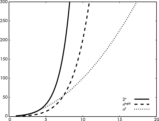
Figure 9-2: Growth of the 2ⁿ, n^log(n), and n² functions, from the fastest to the slowest growing

O(n²) or O(n³) may be efficient, but O(n^99999999999) obviously isn’t. In other words, polytime is fast as long as the exponent isn’t too large. Fortunately, all polynomial-time algorithms found to solve actual problems do have small exponents. For example, O(n^1.465) is the time for multiplying two n-bit integers, or O(n^2.373) for multiplying two n × n matrices. The 2002 breakthrough polytime algorithm for identifying prime numbers initially had a complexity O(n¹²), but it was later improved to O(n⁶). Polynomial time thus may not be the perfect definition of a practical time for an algorithm, but it’s the best we have.

By extension, a problem that can’t be solved by a polynomial-time algorithm is considered impractical, or hard. For example, for a straightforward key search, there’s no way to beat the O(2ⁿ) complexity unless the cipher is somehow broken.

We know for sure that there’s no way to beat the O(2_N) complexity of a brute-force key search (as long as the cipher is secure), but we don’t always know what the fastest way to solve a problem is. A large portion of the research in complexity theory is about proving complexity bounds on the running time of algorithms solving a given problem. To make their job easier, complexity theorists have categorized computational problems in different groups, or classes, according to the effort needed to solve them.

Complexity Classes

In mathematics, a class is a group of objects with some similar attribute. For example, all computational problems solvable in time O(n²), which complexity theorists simply denote TIME(n²), are one class. Likewise, TIME(n³) is the class of problems solvable in time O(n³), TIME(2_N) is the class of problems solvable in time O(2_N), and so on. For the same reason that a supercomputer can compute whatever a laptop can compute, any problem solvable in O(n²) is also solvable in O(n³). Hence, any problem in the class TIME(n²) also belongs to the class TIME(n³), which both also belong to the class TIME(n⁴), and so on. The union of all these classes of problems, TIME(n^k), where k is a constant, is called P, which stands for polynomial time.

If you’ve ever programmed a computer, you’ll know that seemingly fast algorithms may still crash your system by eating all its memory resources. When selecting an algorithm, you should not only consider its time complexity but also how much memory it uses, or its space complexity. This is especially important because a single memory access is usually orders of magnitudes slower than a basic arithmetic operation in a CPU.

Formally, you can define an algorithm’s memory consumption as a function of its input length, n, in the same way we defined time complexity. The class of problems solvable using f(n) bits of memory is SPACE(f(n)). For example, SPACE(n³) is the class of problems solvable using of the order of n³ bits of memory. Just as we had P as the union of all TIME(n^k), the union of all SPACE(n^k) problems is called PSPACE.

Obviously, the lower the memory the better, but a polynomial amount of memory doesn’t necessarily imply that an algorithm is practical. Why? Well, take for example a brute-force key search: again, it takes only negligible memory but is slow as hell. More generally, an algorithm can take forever, even if it uses just a few bytes of memory.

Any problem solvable in time f(n) needs at most f(n) memory, so TIME(f(n)) is included in SPACE(f(n)). In time f(n), you can only write up to f(n) bits, and no more, because writing (or reading) 1 bit is assumed to take one unit of time; therefore, any problem in TIME(f(n)) can’t use more than f(n) space. As a consequence, P is a subset of PSPACE.

Nondeterministic Polynomial Time

NP is the second most important complexity class, after the class P of all polynomial-time algorithms. No, NP doesn’t stand for non-polynomial time, but for nondeterministic polynomial time. What does that mean?

NP is the class of problems for which a solution can be verified in polynomial time—that is, efficiently—even though the solution may be hard to find. By verified, I mean that given a potential solution, you can run some polynomial-time algorithm that will verify whether you’ve found an actual solution. For example, the problem of recovering a secret key with a known plaintext is in NP, because given P, C = E(K, P), and some candidate key K₀, you can check that K₀ is the correct key by verifying that E(K₀, P) equals C. The process of finding a potential key (the solution) can’t be done in polynomial time, but checking whether the key is correct is done using a polynomial-time algorithm.

Now for a counterexample: what about known-ciphertext attacks? This time, you only get some E(K, P) values for random unknown plaintext Ps. If you don’t know what the Ps are, then there’s no way to verify whether a potential key, K₀, is the right one. In other words, the key-recovery problem under known-ciphertext attacks is not in NP (let alone in P).

Another example of a problem not in NP is that of verifying the absence of a solution to a problem. Verifying that a solution is correct boils down to computing some algorithm with the candidate solution as an input and then checking the return value. However, to verify that no solution exists, you may need to go through all possible inputs. And if there’s an exponential number of inputs, you won’t be able to efficiently prove that no solution exists. The absence of a solution is hard to show for the hardest problems in the class NP—the so-called NP-complete problems, which we’ll discuss next.

NP-Complete Problems

The hardest problems in the class NP are called NP-complete; we don’t know how to solve these problems in polynomial time. And as complexity theorists discovered in the 1970s when they developed the theory of NP-completeness, NP’s hardest problems are all equally hard. This was proven by showing that any efficient solution to any of the NP-complete problems can be turned into an efficient solution for any of the other NP-complete problems. In other words, if you can solve any NP-complete problem efficiently, you can solve all of them, as well as all problems in NP. How can this be?

NP-complete problems come in different disguises, but they’re fundamentally similar from a mathematical perspective. In fact, you can reduce any NP-complete problem to any other NP-complete problem such that solving the first one depends on solving the second.

Here are some examples of NP-complete problems:

The traveling salesman problem Given a set of points on a map (cities, addresses, or other geographic locations) and the distances between each point from each other point, find a path that visits every point such that the total distance is smaller than a given distance of x.

The clique problem Given a number, x, and a graph (a set of nodes connected by edges, as in Figure 9-3), determine if there’s a set of x points or less such that all points are connected to each other.

The knapsack problem Given two numbers, x and y, and a set of items, each of a known value and weight, can we pick a group of items such that the total value is at least x and the total weight at most y?

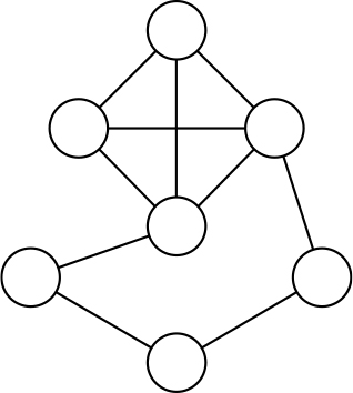
Figure 9-3: A graph containing a clique of four points. The general problem of finding a clique (set of nodes all connected to each other) of given size in a graph is NP-complete.

Such NP-complete problems are found everywhere, from scheduling problems (given jobs of some priority and duration, and one or more processors, assign jobs to the processors by respecting the priority while minimizing total execution time) to constraint-satisfaction problems (determine values that satisfy a set of mathematical constraints, such as logical equations). Even the task of winning in certain video games can sometimes be proven to be NP-complete (for famous games including Tetris, Super Mario Bros., Pokémon, and Candy Crush Saga). For example, the article “Classic Nintendo Games Are (Computationally) Hard” (https://arxiv.org/abs/1203.1895) considers “the decision problem of reachability” to determine the possibility of reaching the goal point from a particular starting point.

Some of these video game problems are actually even harder than NP-complete and are called NP-hard. We say that a problem is NP-hard when it’s at least as hard as NP-complete problems. More formally, a problem is NP-hard if what it takes to solve it can be proven to also solve NP-complete problems.

I have to mention an important caveat. Not all instances of NP-complete problems are actually hard to solve. Some specific instances, because they’re small or because they have a specific structure, may be solved efficiently. Take, for example, the graph in Figure 9-3. By just looking at it for a few seconds you’ll spot the clique, which is the top four connected nodes—even though the aforementioned clique problem is NP-hard, there’s nothing hard here. So being NP-complete doesn’t mean that all instances of a given problem are hard, but that as the problem size grows, many of them are.

The P vs. NP Problem

If you could solve the hardest NP problems in polynomial time, then you could solve all NP problems in polynomial time, and therefore NP would equal P. That sounds preposterous; isn’t it obvious that there are problems for which a solution is easy to verify but hard to find? For example, isn’t it obvious that exponential-time brute force is the fastest way to recover the key of a symmetric cipher, and therefore that the problem can’t be in P? It turns out that, as crazy as it sounds, no one has proved that P is different from NP, despite a bounty of literally one million dollars.

The Clay Mathematics Institute will award this bounty to anyone who proves that either P ≠ NP or P = NP. This problem, known as P vs. NP, was called “one of the deepest questions that human beings have ever asked” by renowned complexity theorist Scott Aaronson. Think about it: if P were equal to NP, then any easily checked solution would also be easy to find. All cryptography used in practice would be insecure, because you could recover symmetric keys and invert hash functions efficiently.

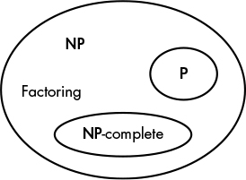
Figure 9-4: The classes NP, P, and the set of NP-complete problems

But don’t panic: most complexity theorists believe P isn’t equal to NP, and therefore that P is instead a strict subset of NP, as Figure 9-4 shows, where NP-complete problems are another subset of NP not overlapping with P. In other words, problems that look hard actually are hard. It’s just difficult to prove this mathematically. While proving that P = NP would only need a polynomial-time algorithm for an NP-complete problem, proving the nonexistence of such an algorithm is fundamentally harder. But this didn’t stop wacky mathematicians from coming up with simple proofs that, while usually obviously wrong, often make for funny reads; for an example, see “The P-versus-NP page” (https://www.win.tue.nl/~gwoegi/P-versus-NP.htm).

Now if we’re almost sure that hard problems do exist, what about leveraging them to build strong, provably secure crypto? Imagine a proof that breaking some cipher is NP-complete, and therefore that the cipher is unbreakable as long as P isn’t equal to NP. But reality is disappointing: NP-complete problems have proved difficult to use for crypto purposes because the very structure that makes them hard in general can make them easy in specific cases—cases that sometimes occur in crypto. Instead, cryptography often relies on problems that are probably not NP-hard.

The Factoring Problem

The factoring problem consists of finding the prime numbers p and q given a large number, N = p × q. The widely used RSA algorithms are based on the fact that factoring a number is difficult. In fact, the hardness of the factoring problem is what makes RSA encryption and signature schemes secure. But before we see how RSA leverages the factoring problem in Chapter 10, I’d like to convince you that this problem is indeed hard, yet probably not NP-complete.

First, some kindergarten math. A prime number is a number that isn’t divisible by any other number but itself and 1. For example, the numbers 3, 7, and 11 are prime; the numbers 4 = 2 × 2, 6 = 2 × 3, and 12 = 2 × 2 × 3 are not prime. A fundamental theorem of number theory says that any integer number can be uniquely written as a product of primes, a representation called the factorization of that number. For example, the factorization of 123456 is 2⁶ × 3 × 643; the factorization of 1234567 is = 127 × 9721; and so on. Any integer has a unique factorization, or a unique way to write it as a product of prime numbers. But how do we know that a given factorization contains only prime numbers or that a given number is prime? The answer is found through polynomial-time primality testing algorithms, which allow us to efficiently test whether a given number is prime. Getting from a number to its prime factors, however, is another matter.

Factoring Large Numbers in Practice

So how do we go from a number to its factorization—namely, its decomposition as a product of prime numbers? The most basic way to factor a number, N, is to try dividing it by all the numbers lower than it until you find a number, x, that divides N. Then attempt to divide N with the next number, x + 1, and so on. You’ll end up with a list of factors of N. What’s the time complexity of this? First, remember that we express complexities as a function of the input’s length. The bit length of the number N is n = log₂ N. By the basic definition of logarithm, this means that N = 2_N. Because all the numbers less than N/2 are reasonable guesses for possible factors of N, there are about N/2 = 2_N/2 values to try. The complexity of our naive factoring algorithm is therefore O(2_N), ignoring the 1/2 coefficient in the O() notation.

Of course, many numbers are easy to factor by first finding any small factors (2, 3, 5, and so on) and then iteratively factoring any other nonprime factors. But here we’re interested in numbers of the form N = p × q, where p and q are large, as found in cryptography.

Let’s be a bit smarter. We don’t need to test all numbers lower than N/2, but rather only the prime numbers, and we can start by trying only those smaller than the square root of N. Indeed, if N is not a prime number, then it has to have at least one factor lower than its square root √N. This is because if both of N’s factors p and q are greater than √N, then their product would be greater than √N × √N = N, which is impossible. For example, if we say N = 100, then its factors p and q can’t both be greater than 10 because that would result in a product greater than 100. Either p or q has to be smaller than √N.

So what’s the complexity of testing only the primes less than √N? The prime number theorem states that there are approximately N/log N primes less than N. Hence, there are approximately √N/log √N primes less than √N. Expressing this value, we get approximately 2^n/2/n possible prime factors and therefore a complexity of O(2^n/2/n), since √N = 2^n/2 and 1/log√N = 1/(n/2) = 2n. This is faster than testing all prime numbers, but it’s still painfully slow—on the order of 2¹²⁰ operations for a 256-bit number. That’s quite an impractical computational effort.

The fastest factoring algorithm is the general number field sieve (GNFS), which I won’t describe here because it requires the introduction of several advanced mathematical concepts. A rough estimate of GNFS’s complexity is exp(1.91 × n^1/3 (log n)^2/3), where exp(. . .) is just a different notation for the exponential function e^x, with e the exponential constant approximately equal to 2.718. However, it’s difficult to get an accurate estimate of GNFS’s actual complexity for a given number size. Therefore, we have to rely on heuristical complexity estimates, which show how security increases with a longer n. For example:

• Factoring a 1024-bit number, which would have two prime factors of approximately 500 bits each, will take on the order of 2⁷⁰ basic operations.
• Factoring a 2048-bit number, which would have two prime factors of approximately 1000 bits each, will take on the order of 2⁹⁰ basic operations, which is about a million times slower than for a 1024-bit number.

And we estimate that at least 4096 bits are needed to reach 128-bit security. Note that these values should be taken with a grain of salt, and researchers don’t always agree on these estimates. Take a look at these experimental results to see the actual cost of factoring:

• In 2005, after about 18 months of computation—and thanks to the power of a cluster of 80 processors, with a total effort equivalent to 75 years of computation on a single processor—a group of researchers factored a 663-bit (200-decimal digit) number.
• In 2009, after about two years and using several hundred processors, with a total effort equivalent to about 2,000 years of computation on a single processor, another group of researchers factored a 768-bit (232-decimal digit) number.

As you can see, the numbers actually factored by academic researchers are shorter than those in real applications, which are at least 1024-bit and often more than 2048-bit. As I write this, no one has reported the factoring of a 1024-bit number, but many speculate that well-funded organizations such as the NSA can do it.

In sum, 1024-bit RSA should be viewed as insecure, and RSA should be used with at least a 2048-bit value—and preferably a 4096-bit one to ensure higher security.

Is Factoring NP-Complete?

We don’t know how to factor large numbers efficiently, which suggests that the factoring problem doesn’t belong to P. However, factoring is clearly in NP, because given a factorization, we can verify the solution by checking that all factors are prime numbers, thanks to the aforementioned primality testing algorithm, and that when multiplied together, the factors do give the expected number. For example, to check that 3 × 5 is the factorization of 15, you’ll check that both 3 and 5 are prime and that 3 times 5 equals 15.

So we have a problem that is in NP and that looks hard, but is it as hard as the hardest NP problems? In other words, is factoring NP-complete? Spoiler alert: probably not.

There’s no mathematical proof that factoring isn’t NP-complete, but we have a few pieces of soft evidence. First, all known NP-complete problems can have one solution, but can also have more than one solution, or no solution at all. In contrast, factoring always has exactly one solution. Also, the factoring problem has a mathematical structure that allows for the GNFS algorithm to significantly outperform a naive algorithm, a structure that NP-complete problems don’t have. Factoring would be easy if we had a quantum computer, a computing model that exploits quantum mechanical phenomena to run different kinds of algorithms and that would have the capability to factor large numbers efficiently (not because it’d run the algorithm faster, but because it could run a quantum algorithm dedicated to factoring large numbers). A quantum computer doesn’t exist yet, though—and might never exist. Regardless, a quantum computer would be useless in tackling NP-complete problems because it’d be no faster than a classical one (see Chapter 14).

Factoring may then be slightly easier than NP-complete in theory, but as far as cryptography is concerned, it’s hard enough, and even more reliable than NP-complete problems. Indeed, it’s easier to build cryptosystems on top of the factoring problem than NP-complete problems, because it’s hard to know exactly how hard it is to break a cryptosystem based on some NP-complete problems—in other words, how many bits of security you’d get.

The factoring problem is just one of several problems used in cryptography as a hardness assumption, which is an assumption that some problem is computationally hard. This assumption is used when proving that breaking a cryptosystem’s security is at least as hard as solving said problem. Another problem used as a hardness assumption, the discrete logarithm problem (DLP), is actually a family of problems, which we’ll discuss next.

The Discrete Logarithm Problem

The DLP predates the factoring problem in the official history of cryptography. Whereas RSA appeared in 1977, a second cryptographic breakthrough, the Diffie–Hellman key agreement (covered in Chapter 11), came about a year earlier, grounding its security on the hardness of the DLP. Like the factoring problem, the DLP deals with large numbers, but it’s a bit less straightforward—it will take you a few minutes rather than a few seconds to get it and requires a bit more math than factoring. So let me introduce the mathematical notion of a group in the context of discrete logarithms.

What Is a Group?

In mathematical context, a group is a set of elements (typically, numbers) that are related to each other according to certain well-defined rules. An example of a group is the set of nonzero integers (between 1 and p – 1) modulo some prime number p, which we write Z_p^*. For p = 5, we get the group Z₅^* = {1,2,3,4}. In the group Z₅^*, operations are carried out modulo 5; hence, we don’t have 3 × 4 = 12 but instead have 3 × 4 = 2, because 12 mod 5 = 2. We nonetheless use the same sign (×) that we use for normal integer multiplication. Likewise, we also use the exponent notation to denote a group element’s multiplication with itself mod p, a common operation in cryptography. For example, in the context of Z₅^*, 2³ = 2 × 2 × 2 = 3 rather than 8, because 8 mod 5 is equal to 3.

To be a group, a mathematical set should have the following characteristics, called group axioms:

Closure For any two x and y in the group, x × y is in the group too. In Z₅^*, 2 × 3 = 1 (because 6 = 1 mod 5), 2 × 4 = 3, and so on.

Associativity For any x, y, z in the group, (x × y) × z = x × (y × z). In Z₅^*, (2 × 3) × 4 = 1 × 4 = 2 × (3 × 4) = 2 × 2 = 4.

Identity existence There’s an element e such that e × x = x × e = x. In any Z_p^*, the identity element is 1.

Inverse existence For any x in the group, there’s a y such that x × y = y × x = e. In Z₅^*, the inverse of 2 is 3, and the inverse of 3 is 2, while 4 is its own inverse because 4 × 4 = 16 = 1 mod 5.

In addition, a group is called commutative if x × y = y × x for any group elements x and y. That’s also true for any multiplicative group of integers Z_p^*. In particular, Z₅^* is commutative: 3 × 4 = 4 × 3, 2 × 3 = 3 × 2, and so on.

A group is called cyclic if there’s at least one element g such that its powers (g¹, g², g³, and so on) mod p span all distinct group elements. The element g is then called a generator of the group. Z₅^* is cyclic and has two generators, 2 and 3, because 2¹ = 2, 2² = 4, 2³ = 3, 2⁴ = 1, and 3¹ = 3, 3² = 4, 3³ = 2, 3⁴ = 1.

Note that I’m using multiplication as a group operator, but you can also get groups from other operators. For example, the most straightforward group is the set of all integers, positive and negative, with addition as a group operation. Let’s check that the group axioms hold with addition, in the preceding order: clearly, the number x + y is an integer if x and y are integers (closure); (x + y) + z = x + (y + z) for any x, y, and z (associativity); zero is the identity element; and the inverse of any number x in the group is –x because x + (–x) = 0 for any integer x. A big difference, though, is that this group of integers is of infinite size, whereas in crypto we’ll only deal with finite groups, or groups with a finite number of elements. Typically, we’ll use groups Z_p^*, where p is thousands of bits long (that is, groups that contain on the order of 2_p numbers).

The Hard Thing

The DLP consists of finding the y for which g^y = x, given a base number g within some group Z_p^*, where p is a prime number, and given a group element x. The DLP is called discrete because we’re dealing with integers as opposed to real numbers (continuous), and it’s called a logarithm because we’re looking for the logarithm of x in base g. (For example, the logarithm of 256 in base 2 is 8 because 2⁸ = 256.)

People often ask me whether factoring or a discrete logarithm is more secure—or in other words, which problem is the hardest? My answer is that they’re about equally hard. In fact, algorithms to solve DLP bear similarities with those factoring integers, and you get about the same security level with n-bit hard-to-factor numbers as with discrete logarithms in an n-bit group. And for the same reason as factoring, DLP isn’t NP-complete. (Note that there are certain groups where the DLP is easier to solve, but here I’m only referring to the case of DLP groups consisting of a number modulo a prime.)

How Things Can Go Wrong

More than 40 years later, we still don’t know how to efficiently factor large numbers or solve discrete logarithms. Amateurs may argue that someone may eventually break factoring—and we have no proof that it’ll never be broken—but we also don’t have proof that P ≠ NP. Likewise, you can speculate that P may be equal to NP; however, according to experts, that surprise is unlikely. So there’s no need to worry. And indeed all the public-key crypto deployed today relies on either factoring (RSA) or DLP (Diffie–Hellman, ElGamal, elliptic curve cryptography). However, although math may not fail us, real-world concerns and human error can sneak in.

When Factoring Is Easy

Factoring large numbers isn’t always hard. For example, take the 1024-bit number N, which is equal to the following:

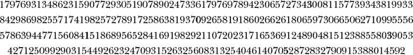
For 1024-bit numbers used in RSA encryption or signature schemes where N = pq, we expect the best factoring algorithms to need around 2⁷⁰ operations, as we discussed earlier. But you can factor this sample number in seconds using SageMath, a piece of Python-based mathematical software. Using SageMath’s factor() function on my 2015 MacBook, it took less than five seconds to find the following factorization:

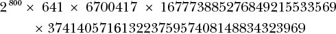
Right, I cheated. This number isn’t of the form N = pq because it doesn’t have just two large prime factors but rather five, including very small ones, which makes it easy to factor. First, you’ll identify the 2⁸⁰⁰ × 641 × 6700417 part by trying small primes from a precomputed list of prime numbers, which leaves you with a 192-bit number that’s much easier to factor than a 1024-bit number with two large factors.

But factoring can be easy not only when n has no small prime factors, but also when N or its factors p and q have particular forms—for example, when N = pq with p and q both close to some 2^b, when N = pq and some bits of p or q are known, or when N is of the form N = p^rq^s and r is greater than log p. However, detailing the reasons for these weaknesses is way too technical for this book.

The upshot here is that the RSA encryption and signature algorithms (covered in Chapter 10) will need to work with a value of N = pq, where p and q are carefully chosen, to avoid easy factorization of N, which can result in security disaster.

Small Hard Problems Aren’t Hard

Computationally hard problems become easy when they’re small enough, and even exponential-time algorithms become practical as the problem size shrinks. A symmetric cipher may be secure in the sense that there’s no faster attack than the 2ⁿ-time brute force, but if the key length is n = 32, you’ll break the cipher in minutes. This sounds obvious, and you’d think that no one would be naive enough to use small keys, but in reality there are plenty of reasons why this could happen. The following are two true stories.

Say you’re a developer who knows nothing about crypto but has some API to encrypt with RSA and has been told to encrypt with 128-bit security. What RSA key size would you pick? I’ve seen real cases of 128-bit RSA, or RSA based on a 128-bit number N = pq. However, although factoring is impractically hard for an N thousands of bits long, factoring a 128-bit number is easy. Using the SageMath software, the commands shown in Listing 9-2 complete instantaneously.

sage: p = random_prime(2**64)
sage: q = random_prime(2**64)
sage: factor(p*q)
6822485253121677229 * 17596998848870549923

Listing 9-2: Generating an RSA modulus by picking two random prime numbers and factoring it instantaneously

Listing 9-2 shows that a 128-bit number taken randomly as the product of two 64-bit prime numbers can be easily factored on a typical laptop. However, if I chose 1024-bit prime numbers instead by using p = random_prime(2**1024), the command factor(p*q) would never complete, at least not in my lifetime.

To be fair, the tools available don’t help prevent the naive use of insecurely short parameters. For example, the OpenSSL toolkit lets you generate RSA keys as short as 31 bits without any warning; obviously, such short keys are totally insecure, as shown in Listing 9-3.

$ openssl genrsa 31
Generating RSA private key, 31 bit long modulus
.+++++++++++++++++++++++++++
.+++++++++++++++++++++++++++
e is 65537 (0x10001)
-----BEGIN RSA PRIVATE KEY-----
MCsCAQACBHHqFuUCAwEAAQIEP6zEJQIDANATAgMAjCcCAwCSBwICTGsCAhpp
-----END RSA PRIVATE KEY-----

Listing 9-3: Generating an insecure RSA private key using the OpenSSL toolkit

When reviewing cryptography, you should not only check the type of algorithms used, but also their parameters and the length of their secret values. However, as you’ll see in the following story, what’s secure enough today may be insecure tomorrow.

In 2015, researchers discovered that many HTTPS servers and email servers still supported an older, insecure version of the Diffie–Hellman key agreement protocol. Namely, the underlying TLS implementation supported Diffie–Hellman within a group, Z_p^*, defined by a prime number, p, of only 512 bits, where the discrete logarithm problem was no longer practically impossible to compute.

Not only did servers support a weak algorithm, but attackers could force a benign client to use that algorithm by injecting malicious traffic within the client’s session. Even better for attackers, the largest part of the attack could be carried out once and recycled to attack multiple clients. After about a week of computations to attack a specific group, Z_p^*, it took only 70 seconds to break individual sessions of different users.

A secure protocol is worthless if it’s undermined by a weakened algorithm, and a reliable algorithm is useless if sabotaged by weak parameters. In cryptography, you should always read the fine print.

For more details about this story, check the research article “Imperfect Forward Secrecy: How Diffie–Hellman Fails in Practice” (https://weakdh.org/imperfect-forward-secrecy-ccs15.pdf).

Further Reading

I encourage you to look deeper into the foundational aspects of computation in the context of computability (what functions can be computed?) and complexity (at what cost?), and how they relate to cryptography. I’ve mostly talked about the classes P and NP, but there are many more classes and points of interest for cryptographers. I highly recommend the book Quantum Computing Since Democritus by Scott Aaronson (Cambridge University Press, 2013). It’s in large part about quantum computing, but its first chapters brilliantly introduce complexity theory and cryptography.

In the cryptography research literature you’ll also find other hard computational problems. I’ll mention them in later chapters, but here are some examples that illustrate the diversity of problems leveraged by cryptographers:

• The Diffie–Hellman problem (given g^x and g ^y, find g^xy) is a variant of the discrete logarithm problem, and is widely used in key agreement protocols.
• Lattice problems, such as the shortest vector problem (SVP) and the learning with errors (LWE) problem, are the only examples of NP-hard problems successfully used in cryptography.
• Coding problems rely on the hardness of decoding error-correcting codes with insufficient information, and have been studied since the late 1970s.
• Multivariate problems are about solving nonlinear systems of equations and are potentially NP-hard, but they’ve failed to provide reliable cryptosystems because hard versions are too big and slow, and practical versions were found to be insecure.

In Chapter 10, we’ll keep talking about hard problems, especially factoring and its main variant, the RSA problem.