Table of Contents for
Applied Text Analysis with Python
 Applied Text Analysis with Python
Published by
O'Reilly Media, Inc., 2018
Applied Text Analysis with Python
Published by
O'Reilly Media, Inc., 2018
- Cover
- nav
- Applied Text Analysis with Python
- Applied Text Analysis with Python
- Preface
- 1. Language and Computation
- 2. Building a Custom Corpus
- 3. Corpus Preprocessing and Wrangling
- 4. Text Vectorization and Transformation Pipelines
- 5. Classification for Text Analysis
- 6. Clustering for Text Similarity
- 7. Context-Aware Text Analysis
- 8. Text Visualization
- 9. Graph Analysis of Text
- 10. Chatbots
- 11. Scaling Text Analytics with Multiprocessing and Spark
- 12. Deep Learning and Beyond
- Glossary
- Index
- About the Authors
- Colophon
Chapter 12. Deep Learning and Beyond
In this book, we have made an effort to emphasize techniques and tools that are sufficiently robust to support practical applications. At times this has meant skimming over promising though less mature libraries and those intended primarily for individual research. Instead, we have favored tools that scale easily from ad hoc analyses on a single machine to large clusters managing interactions for many hundreds of thousands of users. In the last chapter, we explored several such tools, from the Python multiprocessing library to the powerhouse Spark, which enable us to run many models in parallel, and do so rapidly enough to engage large-scale production applications. In this chapter we will discuss an equally significant advancement, neural networks, which are quickly becoming the new state of the art in natural language processing.
Ironically, neural networks are in some sense one of the most “old school” technologies covered in this book, with computational roots dating back to work done nearly 70 years ago. For most of this history, neural networks could not have been considered a practical machine learning method. However, this has changed rapidly over the last two decades thanks to three main advances: first, the dramatic increases in compute power made possible with GPUs and distributed computing in the early 2000s; then, the optimizations in learning rates over the last decade, which we’ll discuss later in the chapter; and finally, with the open source Python libraries like PyTorch, TensorFlow, and Keras that have been made available in the last few years.
A full discussion of these advances is well beyond the scope of this book, but here we will provide a brief overview of neural networks as they relate to the machine learning model families explored in Chapters 5 through 9. We will work through a case study of a sentiment classification problem particularly well-suited to the neural network model family, and finally, discuss present and future trajectories in this area.
Applied Neural Networks
As application developers, we tend to be cautiously optimistic about the kinds of bleeding-edge technologies that sound good on paper but can lead to headaches when it comes to operationalization. For this reason, we feel compelled to begin this chapter with a justification of why we’ve chosen to end this book with a chapter on neural networks.
The current trade-offs between traditional models and neural networks concern two factors: model complexity and speed. Because neural networks tend to take longer to train, they can impede rapid iteration through the workflow discussed in Chapter 5. Neural networks are also typically more complex than traditional models, meaning that their hyperparameters are more difficult to tune and modeling errors are more challenging to diagnose.
However, neural networks are not only increasingly practical, they also promise nontrivial performance gains over traditional models. This is because unlike traditional models, which face performance plateaus even as more data become available, neural models continue to improve.
Neural Language Models
In Chapter 7, we introduced the notion that a language model could be learned from a sufficiently large and domain-specific corpus using a probabilistic model. This is known as a symbolic model of language. In this chapter we consider a different approach: the neural or connectionist language model.
The connectionist model of language argues that the units of language interact with each other in meaningful ways that are not necessarily encoded by sequential context. For instance, the contextual relationship of words may be sequential, but may also be separated by other phrases, as we see in Figure 12-1. In the first example, a successful symbolic model would assign high probabilities to “heard,” “listened to,” and “purchased.” However, in the second example, it would be difficult for our model to predict the next word, which depends on knowledge that “Yankee Hotel Foxtrot,” mentioned in the earlier part of the sentence, is an album.
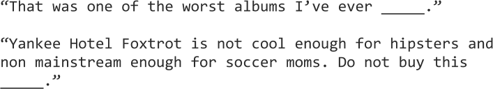
Figure 12-1. Nonsequential context
Since many interactions are not directly interpretable, some intermediary representation must be used to describe the connections, and connectionist models tend to use artificial neural networks (ANNs) or Bayesian networks to learn the underlying relationships.
Traditional symbolic models require significant engineering effort to manage n-gram smoothing and backoff, and can suffer from the requisite RAM needed to hold so many n-grams in memory. Connectionist models, on the other hand, approach the problem by scaling model complexity. In fact, the primary benefit of a neural model approach is to avoid lengthy feature engineering because neural models create infinitely smoothed functions from large arbitrary inputs.
In the next few sections, we will discuss some of the types of neural networks, unpack their components, and demonstrate how a connectionist model might be implemented in an applied context—in this case, to perform sentiment analysis.
Artificial Neural Networks
Neural networks comprise a very broad and variegated family of models, but are more or less all evolved from the perceptron, a linear classification machine developed in the late 1950s by Frank Rosenblatt at Cornell and modeled on the learning behavior of the human brain.
At the core of the neural network model family are several components, as shown in Figure 12-2—an input layer, a vectorized first representation of the data, a hidden layer consisting of neurons and synapses, and an output layer containing the predicted values. Within the hidden layer, synapses are responsible for transmitting signals between the neurons, which rely on a nonlinear activation function to buffer those incoming signals. The synapses apply weights to incoming values, and the activation function determines if the weighted inputs are sufficiently high to activate the neuron and pass the values on to the next layer of the network.
In a feedforward network, signals travel from the input to the output layer in a single direction. In more complex architectures like recurrent and recursive networks, signal buffering can combine or recur between the nodes within a layer.
Note
There are many variations on activation functions, but generally it makes sense to use a nonlinear one, which allows the neural network to model more complex decision spaces. Sigmoidal functions are very common, though they can make gradient descent slow when the slope is almost zero. For this reason, rectified linear units or “ReLUs,” which output the sum of the weighted inputs (or zero if that sum is negative), have become increasingly popular.
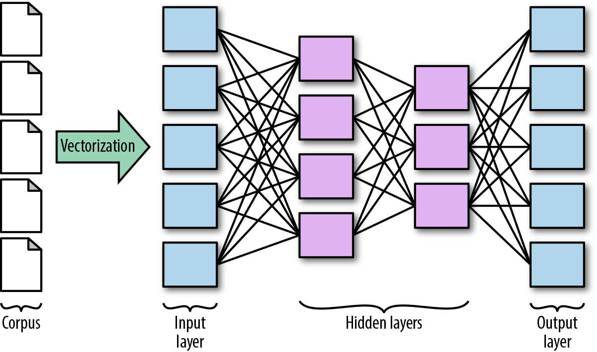
Figure 12-2. Neural model components
Backpropagation is the process by which error, computed at the final layer of the network, is communicated back through the layers to incrementally adjust the synapse weights and improve accuracy in the next training iteration. After each iteration, the model calculates the gradient of the loss function to determine the direction in which to adjust the weights.
Training a multilayer perceptron
Multilayer perceptrons are one of the simplest forms of feedforward artificial neural networks. In this section, we will train a multilayer perceptron using the Scikit-Learn library.
Our input data is a series of 18,000 reviews of albums from the website Pitchfork.com1; each review contains the text of the review, in which the music reviewer discusses the relative merits of the album and the band, as well as a floating-point numeric score between 0 and 10. An excerpt2 can be seen in Figure 12-3.
We would like to predict the relative positivity or negativity of a review given the text. Scikit-Learn’s neural net module, sklearn.neural_network, enables us to train a multilayer perceptron to perform classification or regression using the now familiar fit and predict methods. We’ll attempt both a regression to predict the actual numeric score of an album and a classification to predict if the album is “terrible,” “okay,” “good,” or “amazing.”
Figure 12-3. Sample Pitchfork review
First, we create a function, documents, to retrieve the pickled, part-of-speech tagged documents from our corpus reader object, a continuous function to get the original numeric ratings of each album, and a categorical function that uses NumPy’s digitize method to bin the ratings into our four categories:
importnumpyasnpdefdocuments(corpus):returnlist(corpus.reviews())defcontinuous(corpus):returnlist(corpus.scores())defmake_categorical(corpus):"""terrible : 0.0 < y <= 3.0okay : 3.0 < y <= 5.0great : 5.0 < y <= 7.0amazing : 7.0 < y <= 10.1"""returnnp.digitize(continuous(corpus),[0.0,3.0,5.0,7.0,10.1])
Next, we add a train_model function, which will take as input a path to the pickled corpus, a Scikit-Learn estimator, and keyword arguments for whether the labels are continuous, an optional path for storing the fitted model, and the number of folds to use in cross-validation.
Our function instantiates a corpus reader, calls the documents function as well as either continuous or make_categorical to get the input values X and the target values y. We then calculate the cross-validated scores, fit and store the model using the joblib utility from Scikit-Learn, and return the scores:
fromsklearn.externalsimportjoblibfromsklearn.model_selectionimportcross_val_scoredeftrain_model(path,model,continuous=True,saveto=None,cv=12):"""Trains model from corpus at specified path; constructing cross-validationscores using the cv parameter, then fitting the model on the full data.Returns the scores."""# Load the corpus data and labels for classificationcorpus=PickledReviewsReader(path)X=documents(corpus)ifcontinuous:y=continuous(corpus)scoring='r2_score'else:y=make_categorical(corpus)scoring='f1_score'# Compute cross-validation scoresscores=cross_val_score(model,X,y,cv=cv,scoring=scoring)# Write to disk if specifiedifsaveto:joblib.dump(model,saveto)# Fit the model on entire datasetmodel.fit(X,y)# Return scoresreturnscores
Note
As with other Scikit-Learn estimators, MLPRegressor and MLPClassifier expect NumPy arrays of floating-point values, and while arrays can be dense or sparse, it’s best to scale input vectors using one-hot encoding or a standardized frequency encoding.
To create our models for training, we will build two pipelines to streamline the text normalization, vectorization, and modeling steps:
if__name__=='__main__':fromtransformerimportTextNormalizerfromreaderimportPickledReviewsReaderfromsklearn.pipelineimportPipelinefromsklearn.neural_networkimportMLPRegressor,MLPClassifierfromsklearn.feature_extraction.textimportTfidfVectorizer# Path to postpreprocessed, part-of-speech tagged review corpuscpath='../review_corpus_proc'regressor=Pipeline([('norm',TextNormalizer()),('tfidf',TfidfVectorizer()),('ann',MLPRegressor(hidden_layer_sizes=[500,150],verbose=True))])regression_scores=train_model(cpath,regressor,continuous=True)classifier=Pipeline([('norm',TextNormalizer()),('tfidf',TfidfVectorizer()),('ann',MLPClassifier(hidden_layer_sizes=[500,150],verbose=True))])classifer_scores=train_model(cpath,classifier,continuous=False)
Note
Similar to choosing k for k-means clustering, selecting the best number and size of hidden layers in an initial neural network prototype is more art than science. The more layers and more nodes per layer, the more complex our model will be, and more complex models require more training data. A good rule of thumb is to start with a simple model (our initial layer should not contain more nodes than we have instances, and should consist of no more than two layers), and iteratively add complexity while using k-fold cross-validation to detect overfit.
Scikit-Learn provides many features for tuning neural networks and can be customized. For example, by default, both MLPRegressor and MLPClassifier use the ReLU activation function, which can be specified with the activation param, and stochastic gradient descent to minimize the cost function, which can be specified with the solver param:
Mean score for MLPRegressor: 0.27290534221341
Mean score for MLPClassifier: 0.7115215174722
The MLPRegressor is fairly weak, showing a very low goodness of fit to the data as described by the R2 score. Regression benefits from reducing the number of dimensions particularly with respect to the number of instances. We can reason about this through the lens of the curse of dimensionality; the Pitchfork reviews are on average about 1,000 words in length, and each word adds another dimension to our decision space. Since our corpus consists of only about 18,000 reviews total, our MLPRegressor simply doesn’t have enough instances to predict scores to the degree of float-point numeric precision.
However, we can see that the MLPClassifier has much better results, and is probably worth additional tuning. To improve our MLPClassifier’s performance, we can experiment with adding and removing complexity. We can add complexity by adding more layers and neurons to hidden_layer_sizes. We can also increase the max_iter param to increase the number of training epochs and give our model more time to learn from backpropagation.
We can also decrease the complexity of the model by removing layers, decreasing the number of neurons, or adding a regularization term to the loss function using the alpha param, which, similar to a sklearn.linear_model.RidgeRegression, will artificially shrink the parameters to help prevent overfitting.
Using the Scikit-Learn API to construct neural models is very convenient for simple models. However, as we will see in the next section, libraries like TensorFlow provide much more in the way of flexibility and tuning of the model architecture, as well as speed, leveraging GPUs to scale for higher performance on larger datasets.
Deep Learning Architectures
Frequently grouped together by the term deep learning, models such as recurrent neural networks (RNNs), long short-term memory networks (LSTMs), recursive neural tensor networks (RNTNs), convolutional neural networks (CNNs or ConvNets), and generative adversarial networks (GANs) have become increasingly popular in recent years.
While people generally define deep neural networks as neural networks with multiple hidden layers, the term “deep learning” is really not meaningfully distinct from modern ANNs. However, different architectures do implement unique functionalities within the layers that enable them to model very complex data.
Convolutional neural networks (CNNs), for instance, combine multilayer perceptrons with a convolutional layer that iteratively builds a map to extract important features, as well as a pooling stage that reduces the dimensionality of the features but preserves their most informative components. CNNs are highly effective for modeling image data and performing tasks like classification and summarization.
For modeling sequential language data, variations on recurrent neural nets (RNNs) like long short-term memory (LSTM) networks have been shown to be particularly effective. The architecture of an RNN allows the model to maintain the order of words in the sequence and to keep track of long-term dependencies. LSTMs, for example, implement gated cells that allow for functions like “memory” and “forgetting.” Variants of this model are very popular for machine translation and natural language generation tasks.
TensorFlow: A framework for deep learning
TensorFlow is a distributed computation engine that exposes a framework for deep learning. Developed by Google for the purpose of parallelizing models across not only GPUs but also networks of many machines, it was made open source in November 2015 and has since become one of the most popular publicly available deep learning libraries.
TensorFlow presumes the user has fairly substantial familiarity with neural network architectures, and is geared toward building data flow graphs with a significant degree of customization. In the TensorFlow workflow, we begin by specifying each layer and all hyperparameters, then compile those steps into a static graph, and then run a session to begin the training. While this makes deep learning models easier to control and optimize as their complexity increases, it also makes rapid prototyping much more challenging.
In essence, deep learning models are just chains of functions, which means that many deep learning libraries tend to have a functional or verbose, declarative style. As such, an ecosystem of other libraries, including Keras, TF-slim, TFLearn, and SkFlow, have quickly evolved to provide a more abstract, object-oriented interface for deep learning. In the next section, we will demonstrate how to use TensorFlow through the Keras API.
Keras: An API for deep learning
While it is often grouped together with deep learning frameworks like TensorFlow, Caffe, Theano, and PyTorch, Keras exposes a general API spec for deep learning. The original Keras interface was written for a Theano backend, but following TensorFlow’s open sourcing and dramatic popularity, the Keras API quickly became the default for many TensorFlow users, and was pulled into the TensorFlow core in early 2017.
In Keras, everything is an object, which makes it a particularly convenient tool for prototyping. In order to roughly recreate the multilayer perceptron classifier we used in the previous section, we can create a build_network function that instantiates a Sequential Keras model, adds two Dense (meaning fully connected) hidden layers, the first with 500 nodes and the second with 150, and both of which employ rectified linear units for the activation parameter. Note that in our first hidden layer, we are required to pass in a tuple, input_shape for the shape of the input layer.
In the output layer we must specify a function to condense the dimensions of the previous layer into the same space as the number of classes in our classification problem. In this case we use softmax, a popular choice for natural language processing because it represents a categorical distribution that aligns with the tokens of our corpus. The build_network function then calls the compile method, specifying the desired loss and optimizer functions for gradient descent, and finally returns the compiled network:
fromkeras.layersimportDensefromkeras.modelsimportSequentialN_FEATURES=5000N_CLASSES=4defbuild_network():"""Create a function that returns a compiled neural network"""nn=Sequential()nn.add(Dense(500,activation='relu',input_shape=(N_FEATURES,)))nn.add(Dense(150,activation='relu'))nn.add(Dense(N_CLASSES,activation='softmax'))nn.compile(loss='categorical_crossentropy',optimizer='adam',metrics=['accuracy'])returnnn
The keras.wrappers.scikit_learn module exposes KerasClassifier and KerasRegressor, two wrappers that implement the Scikit-Learn interface. This means that we can incorporate Sequential Keras models as part of a Scikit-Learn Pipeline or Gridsearch.
To use the KerasClassifier in our workflow, we begin our pipeline as in the previous section, with a TextNormalizer (as described in “Creating a custom text normalization transformer”) and a Scikit-Learn TfidfVectorizer. We use the vectorizer’s max_features parameter to pass in the N_FEATURES global variable, which will ensure our vectors have the same dimensionality as our compiled neural network’s input_shape.
Warning
For those of us spoiled by Scikit-Learn estimators, which are flush with sensible default hyperparameters, building deep learning models can be a bit frustrating at first. Keras and TensorFlow assume very little about the size and shape of your incoming data, and will not intuit the hyperparameters of the decision space. Nevertheless, learning to construct TensorFlow models via the Keras API enables us not only to build custom models, but also to train them in a fraction of the time of a sklearn.neural_network model.
Finally, we add the KerasClassifier to the pipeline, passing in the network’s build function, desired number of epochs, and an optional batch size. Note that we must pass build_network in as a function, not as an instance of the compiled network:
if__name__=='__main__':fromsklearn.pipelineimportPipelinefromtransformerimportTextNormalizerfromkeras.wrappers.scikit_learnimportKerasClassifierfromsklearn.feature_extraction.textimportTfidfVectorizerpipeline=Pipeline([('norm',TextNormalizer()),('vect',TfidfVectorizer(max_features=N_FEATURES)),('nn',KerasClassifier(build_fn=build_network,epochs=200,batch_size=128))])
We can now run and evaluate our pipeline using a slightly modified version of our train_model function. Just as in the previous section, this function will instantiate a corpus reader, call documents and make_categorical get the input and target values X and y, compute cross-validated scores, fit and store the model, and return the scores.
Unfortunately, at the time of this writing, pipeline persistence for a Scikit-Learn wrapped Keras model is somewhat challenging, since the neural network component must be saved using the Keras-specific save method as a hierarchical data format (.h5) file. As a workaround, we use Pipeline indexing to store first the trained neural network and then the remainder of the fitted pipeline using joblib:
deftrain_model(path,model,saveto=None,cv=12):"""Trains model from corpus at specified path and fits on full data.If a saveto dictionary is specified, writes Keras and Sklearnpipeline components to disk separately. Returns the scores."""corpus=PickledReviewsReader(path)X=documents(corpus)y=make_categorical(corpus)scores=cross_val_score(model,X,y,cv=cv,scoring='accuracy',n_jobs=-1)model.fit(X,y)ifsaveto:model.steps[-1][1].model.save(saveto['keras_model'])model.steps.pop(-1)joblib.dump(model,saveto['sklearn_pipe'])returnscores
Now, back in our if-main statement, we provide the path to the corpus and the dictionary of paths where our serialized model will be stored:
cpath='../review_corpus_proc'mpath={'keras_model':'keras_nn.h5','sklearn_pipe':'pipeline.pkl'}scores=train_model(cpath,pipeline,saveto=mpath,cv=12)
With 5,000 input features to our neural network, our preliminary Keras classifier performed fairly well; on average, our model is able to predict whether a Pitchfork review considered an album “terrible,” “okay,” “great,” or “amazing”:
Mean score for KerasClassifier: 0.70533893018807
While the mean score of our Scikit-Learn classifier was slightly higher, using Keras, the training took only two hours on a MacBook Pro with all available cores, or roughly one-sixth the training time of the Scikit-Learn MLPClassifier. As a result, we can see that tuning the Keras model (e.g., adding more hidden layers and nodes, adjusting the activation or cost functions, randomly “dropping out,” or setting a fraction of inputs to zero to avoid overfitting, etc.) will allow for more rapid improvements to our model.
However, one of the main challenges for our model is the small size of the dataset; neural networks generally outperform other machine learning model families, but only beyond some threshold of available training data (for more discussion on this, see Andrew Ng’s “Why Is Deep Learning Taking Off?”3). In the next section of this chapter, we will explore a much larger dataset, as well as experimenting with using the kinds of syntactic features we saw in Chapters 7 and 10 to improve the signal-to-noise ratio.
Sentiment Analysis
So far we have been treating our reviews as pure bags of words, which is not uncommon for neural networks. Activation functions typically require input to be in the discrete range of [0,1] or [-1,1], which makes one-hot encoding a convenient vectorization method.
However, the bag-of-words model is problematic for more nuanced text analytics tasks because it captures the broad, most important elements of text rather than the microsignals that describe meaningful adjustments or modifications. Language generation, which we explored briefly in Chapters 7 and 10, is an application for which bag-of-words models are frequently insufficient for capturing the intricacies of human speech patterns. Another such case is sentiment analysis, where the relative positivity or negativity of a statement is a function of a complex interplay between positively and negatively associated modifiers and nonlexical factors like sarcasm, hyperbole, and symbolism.
In Chapter 1 we briefly introduced sentiment analysis to describe the importance of contextual features. Whereas a language feature like gender is often encoded in the structure of language, sentiment is often much too complex to be encoded at the token level. Take, for example, this sample text from a set of Amazon customer reviews of patio, lawn, and garden equipment:
I used to use a really primitive manual edger that I inherited from my father. Blistered hands and time wasted, I decided there had to be a better way and this is surely it. Edging is one of those necessary evils if you want a great looking house. I don’t edge every time I mow. Usually I do it every other time. The first time out after a long winter, edging usually takes a little longer. After that, edging is a snap because you are basically in maintenance mode. I also use this around my landscaping and flower beds with equally great results. The blade on the Edge Hog is easily replaceable and the tell tale sign to replace it is when the edge starts to look a little rough and the machine seems slower.
Amazon reviewer
If we predict the rating using a count of the “positive” and “negative” review words as with the gendered words in Chapter 1, what score would you expect to see? In spite of many of the negative-seeming words (e.g., “primitive,” “blistered,” “wasted,” “rough,” “slower”), this text corresponds to a 5-star review—the highest possible rating!
Even if we were to take a single sentence from the review (e.g., “Edging is one of those necessary evils if you want a great-looking house.”) we can see how positive and negative phrases modify each other, with the effect of sometimes inverting or magnifying the sentiment. The parse tree in Figure 12-4 illustrates how these syntactic chunks combine to influence the overall sentiment of the review.
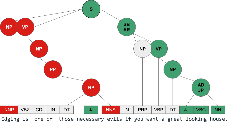
Figure 12-4. Syntax analysis
Deep Structure Analysis
A syntactic chunking approach to sentiment analysis was proposed by Richard Socher (2013).4 Socher et al. propose that sentiment classification using a phrase treebank (i.e., a corpus that has been syntactically annotated) allows for a more nuanced prediction of the overall sentiment of the utterance. They demonstrated how classifying sentiment phrase-by-phrase rather than on the entire utterance level ultimately results in significant improvements in accuracy, particularly because it enables complex modeling of the effects of negation at various levels of the parse tree, as we saw in Figure 12-4.
Socher also introduced a novel approach to neural network modeling, the recursive neural tensor network. Unlike standard feedforward and recurrent models, recursive networks anticipate hierarchical data and a training process that amounts to the traversal of a tree. These models employ embeddings, like those introduced in Chapter 4, to represent words or “leaves” of the tree, along with a compositionality function that determines how the vectorized leaves should be recursively combined to represent the phrases.
Like the KerasClassifier we built earlier in this chapter, recursive neural networks use activation functions in the hidden layers to model nonlinearly, as well as a compression function to reduce the dimensionality of the final layer to match the number of classes (usually two in the case of sentiment analysis), such as softmax.
Note
It’s important to note that the efficacy of Socher’s model is also due in large part to the massive training set. Socher’s team constructed the training data by extracting every syntactically possible phrase from thousands of rottentomatoes.com movie reviews, which were then manually scored by Amazon Mechanical Turk workers via a labeling interface. The results, original Matlab code, and a number of visualizations of sentiment parse trees are available via the Stanford Sentiment Treebank.5
In the next section, we’ll implement a sentiment classifier that borrows some of the ideas from Socher’s work, leveraging the structure of language as a tool for boosting signal.
Predicting sentiment with a bag-of-keyphrases
In the previous section, we used Keras to train a simple multilayer perceptron to fairly successfully predict how a Pitchfork music critic would score an album, based on the words contained in their review. In this section, we’ll attempt to build a more complex model with a larger corpus and a “bag-of-keyphrases” approach.
For our new corpus, we will use a subset of the Amazon product reviews corpus compiled by Julian McAuley of the University of California at San Diego.6 The full dataset contains over one million reviews of movies and television, each of which is comprised of the text of the review and its score. The scores are categorical, ranging from the lowest rating of 1 to the highest rating of 5.
The premise of our model is that most of the semantic information in our text will be contained in small syntactic substructures within the sentences. Instead of using a bag-of-words approach, we will implement a lightweight method to leverage the syntactic structure of our review text by adding a new KeyphraseExtractor class, which will modify the keyphrase extraction technique from Chapter 7 to transform our review corpus documents in a vector representation of the document keyphrases.
In particular, we will use a regular expression to define a grammar that uses the part-of-speech tags to identify adverbial phrases (“without care”) and adjective phrases (“terribly helpful”). We can then chunk our text into keyphrases using the NLTK RegexpParser. We will be using a neural network model that requires us to know in advance the total number of features (in other words, the lexicon) and the length of each document, so we’ll add these parameters to our __init__ function.
Note
Setting hyperparameters for the maximum vocabulary and document length cutoff will depend on the data and require iterative feature engineering. We might begin by computing the total number of unique keywords and setting our nfeatures parameter to be less than that number. For document length, we might count the number of keywords in each document in our corpus and take the mean.
classKeyphraseExtractor(BaseEstimator,TransformerMixin):"""Extract adverbial and adjective phrases, and transformdocuments into lists of these keyphrases, with a totalkeyphrase lexicon limited by the nfeatures parameterand a document length limited/padded to doclen"""def__init__(self,nfeatures=100000,doclen=60):self.grammar=r'KT: {(<RB.> <JJ.*>|<VB.*>|<RB.*>)|(<JJ> <NN.*>)}'self.chunker=RegexpParser(self.grammar)self.nfeatures=nfeaturesself.doclen=doclen
To further reduce complexity, we’ll add a normalize method that removes punctuation from each tokenized, tagged sentence and lowercases the words, and a extract_candidate_phrases that uses our grammar to extract keyphrases from each sentence:
...defnormalize(self,sent):is_punct=lambdaword:all(unicat(c).startswith('P')forcinword)sent=filter(lambdat:notis_punct(t[0]),sent)sent=map(lambdat:(t[0].lower(),t[1]),sent)returnlist(sent)defextract_candidate_phrases(self,sents):"""For a document, parse sentences using our chunker created byour grammar, converting the parse tree into a tagged sequence.Extract phrases, rejoin with a space, and yield the documentrepresented as a list of its keyphrases."""forsentinsents:sent=self.normalize(sent)ifnotsent:continuechunks=tree2conlltags(self.chunker.parse(sent))phrases=[" ".join(wordforword,pos,chunkingroup).lower()forkey,groupingroupby(chunks,lambdaterm:term[-1]!='O')ifkey]forphraseinphrases:yieldphrase
To pass the size of the input layer to our neural network, we use a get_lexicon method to extract the keyphrases from each review and build a lexicon with the desired number of features. Finally, a clip method will ensure each document includes only keyphrases from the lexicon:
...defget_lexicon(self,keydocs):"""Build a lexicon of size nfeatures"""keyphrases=[keyphrasefordocinkeydocsforkeyphraseindoc]fdist=FreqDist(keyphrases)counts=fdist.most_common(self.nfeatures)lexicon=[phraseforphrase,countincounts]return{phrase:idx+1foridx,phraseinenumerate(lexicon)}defclip(self,keydoc,lexicon):"""Remove keyphrases from documents that aren't in the lexicon"""return[lexicon[keyphrase]forkeyphraseinkeydocifkeyphraseinlexicon.keys()]
While our fit method is a no-op, simply returning self, the transform method will do the heavy lifting of extracting the keyphrases, building the lexicons, clipping the documents, and then padding each using Keras’ sequence.pad_sequences function so that they’re all of the same desired length:
fromkeras.preprocessingimportsequence...deffit(self,documents,y=None):returnselfdeftransform(self,documents):docs=[list(self.extract_candidate_phrases(doc))fordocindocuments]lexicon=self.get_lexicon(docs)clipped=[list(self.clip(doc,lexicon))fordocindocs]returnsequence.pad_sequences(clipped,maxlen=self.doclen)
Now we will write a function to build our neural network; in this case we’ll be building a long short-term memory (LSTM) network.
Our LSTM will begin with an Embedding layer that will build a vector embedding from our keyphrase documents, specifying three parameters: the total number of features (e.g., the total size of our keyphrase lexicon), the desired dimensionality of the embeddings, and the input_length of each keyphrase document. Our 200-node LSTM layer is nested between two Dropout layers, which will randomly set a fraction of the input units to 0 during each training cycle to help prevent overfitting. Our final layer specifies the number of expected targets for our sentiment classification:
N_FEATURES=100000N_CLASSES=2DOC_LEN=60defbuild_lstm():lstm=Sequential()lstm.add(Embedding(N_FEATURES,128,input_length=DOC_LEN))lstm.add(Dropout(0.4))lstm.add(LSTM(units=200,recurrent_dropout=0.2,dropout=0.2))lstm.add(Dropout(0.2))lstm.add(Dense(N_CLASSES,activation='sigmoid'))lstm.compile(loss='categorical_crossentropy',optimizer='adam',metrics=['accuracy'])returnlstm
We will be training our sentiment model as a binary classification problem (as Socher did in his implementation), so we will add a binarize function to bin our labels into two categories for use in our train_model function. The two classes will roughly correspond to “liked it” or “hated it”:
defbinarize(corpus):"""hated it : 0.0 < y <= 3.0liked it : 3.0 < y <= 5.1"""returnnp.digitize(continuous(corpus),[0.0,3.0,5.1])deftrain_model(path,model,cv=12,**kwargs):corpus=PickledAmazonReviewsReader(path)X=documents(corpus)y=binarize(corpus)scores=cross_val_score(model,X,y,cv=cv,scoring='accuracy')model.fit(X,y)...returnscores
Finally, we’ll specify our Pipeline input and components, and call our train_model function to get our cross-validated scores:
if__name__=='__main__':am_path='../am_reviews_proc'pipeline=Pipeline([('keyphrases',KeyphraseExtractor()),('lstm',KerasClassifier(build_fn=build_nn,epochs=20,batch_size=128))])scores=train_model(am_path,pipeline,cv=12)
Mean score: 0.8252357452734355
The preliminary results of our model are surprisingly effective, suggesting that keyphrase extraction is a useful way to reduce dimensionality for text data without totally discarding the semantic information encoded in syntactic structures.
The Future Is (Almost) Here
It is an exciting time for text analysis, not only because of the many new industrial applications for machine learning on text, but also thanks to the burgeoning technologies available to support these applications. The hardware advances made over the last few decades, and the corresponding open source implementations made available in the last few years, have moved neural networks from the space of academic research to the realm of practical application. Applied text analyses therefore need to be prepared to integrate new hardware as well as academic research into existing code bases to stay current and relevant. Just as language changes, so too must language processing.
Some of the biggest challenges in natural language processing—machine translation, summarization, paraphrasing, question-and-answer, and dialog—are currently being addressed with neural networks. Increasingly, research efforts in deep learning models for language data endeavor to move from language processing to understanding.
While current commercial applications are very recognizable, they are still relatively few. Technologies such as Alexa’s speech recognition, Google Translate app’s machine translation, and Facebook’s image captioning for visually impaired users are increasingly connecting text, sound, and images in innovative ways. Many of the features that emerge in the next few years will involve algorithmic improvements and hybrid models that, for instance, can combine image classification with natural language generation, or speech recognition with machine translation.
However, we will also begin to see more smaller-scale text analytics developed to subtly improve the user experience of everyday applications—text autocompletion, conversational agents, improved product recommendations, etc. Such applications will rely not (or not exclusively) on massive datasets, but on custom, domain-specific corpora geared to specific use cases.
While there are currently few companies with sufficient data, staff, and high-performance compute power to make applied neural networks practical and cost-effective, this too is changing. However, for the majority of data scientists and applications developers, the future of applied text analysis will be less about algorithmic innovation and more about spotting interesting problems in the wild and applying robust and scalable tools and techniques to build small, but high-value features that differentiate our applications from those of previous generations.
1 Condé Nast, Pitchfork: The Most Trusted Voice In Music, (2018) http://bit.ly/2GNLO7F
2 Larry Fitzmaurice, Review of Coldplay’s Ghost Stories, (2014) http://bit.ly/2GQL1ms
3 Andrew Ng, Why is Deep Learning Taking Off?, (2017) http://bit.ly/2JJ93kU
4 Richard Socher, Alex Perelygin, Jean Y. Wu, Jason Chuang, Christopher D. Manning, Andrew Y. Ng, and Christopher Potts, Recursive Deep Models for Semantic Compositionality Over a Sentiment Treebank, (2013) http://bit.ly/2GQL2Xy
5 Jean Wu, Richard Socher, Rukmani Ravisundaram, and Tayyab Tariq, Stanford Sentiment Treebank, (2013) https://stanford.io/2GQL3uA
6 Julian McAuley, Amazon product data, (2016) http://bit.ly/2GQL2H2