Table of Contents for
Applied Text Analysis with Python
 Applied Text Analysis with Python
Published by
O'Reilly Media, Inc., 2018
Applied Text Analysis with Python
Published by
O'Reilly Media, Inc., 2018
- Cover
- nav
- Applied Text Analysis with Python
- Applied Text Analysis with Python
- Preface
- 1. Language and Computation
- 2. Building a Custom Corpus
- 3. Corpus Preprocessing and Wrangling
- 4. Text Vectorization and Transformation Pipelines
- 5. Classification for Text Analysis
- 6. Clustering for Text Similarity
- 7. Context-Aware Text Analysis
- 8. Text Visualization
- 9. Graph Analysis of Text
- 10. Chatbots
- 11. Scaling Text Analytics with Multiprocessing and Spark
- 12. Deep Learning and Beyond
- Glossary
- Index
- About the Authors
- Colophon
Chapter 9. Graph Analysis of Text
Up until this point, we have been applying traditional classification and clustering algorithms to text. By allowing us to measure distances between terms, assign weights to phrases, and calculate probabilities of utterances, these algorithms enable us to reason about the relationships between documents. However, tasks such as machine translation, question answering, and instruction-following often require more complex, semantic reasoning.
For instance, given a large number of news articles, how would you build a model of the narratives they contain—of actions taken by key players or enacted upon others, of the sequence of events, of cause and effect? Using the techniques in Chapter 7, you could extract the entities or keyphrases or look for themes using the topic modeling methods described in Chapter 6. But to model information about the relationships between those entities, phrases, and themes, you would need a different kind of data structure.
Let’s consider how such relationships may be expressed in the headlines of some of our articles:
headlines=['FDA approves gene therapy','Gene therapy reduces tumor growth','FDA recalls pacemakers']
Traditionally, phrases like these are encoded using text meaning representations (TMRs). TMRs take the form of ('subject', 'predicate', 'object') triples (e.g., ('FDA', 'recalls', 'pacemakers')), to which first-order logic or lambda calculus can be applied to achieve semantic reasoning.
Unfortunately, the construction of TMRs often requires substantial prior knowledge. For instance, we need to know not only that the acronym “FDA” is an actor, but that “recalling” is an action that can be taken by some entities against others. For most language-aware data products, building a sufficient number of TMRs to support meaningful semantic analysis will not be practical.
However, if we shift our thinking slightly, we might also think of this subject-predicate-object as a graph, where the predicates are edges between subject and object nodes, as shown in Figure 9-1. By extracting co-occurring entities and keyphrases from the headlines, we can construct a graph representation of the relationships between the “who,” the “what,” and even the “where,” “how,” and “when” of an event. This will allow us to use graph traversal to answer analytical questions like “Who are the most influential actors to an event?” or “How do relationships change over time?” While not necessarily a complete semantic analysis, this approach can produce useful insights.
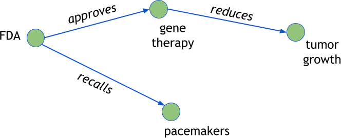
Figure 9-1. Semantic reasoning on text using graphs
In this chapter, we will analyze text data in this way, using graph algorithms. First, we will build a graph-based thesaurus and identify some of the most useful graph metrics. We will then extract a social graph from our Baleen corpus, connecting actors that appear in the same documents together and employing some simple techniques for extracting and analyzing subgraphs. Finally, we will introduce a graph-based approach to entity resolution called fuzzy blocking.
Note
NetworkX and Graph-tool are the two primary Python libraries that implement graph algorithms and the property graph model (which we’ll explore later in this chapter). Graph-tool scales significantly better than NetworkX, but is a C++ implementation that must be compiled from source. For graph-based visualization, we frequently leverage non-Python tools, such as Gephi, D3.js, and Cytoscape.js. To keep things simple in this chapter, we will stick to NetworkX.
Graph Computation and Analysis
One of the primary exercises in graph analytics is to determine what exactly the nodes and edges should be. Generally, nodes represent the real-world entities we would like to analyze, and edges represent the different types (and magnitudes) of relationships that exist between nodes.
Once a schema is determined, graph extraction is fairly straightforward. Let’s consider a simple example that models a thesaurus as a graph. A traditional thesaurus maps words to sets of other words that have similar meanings, connotations, and usages. A graph-based thesaurus, which instead represents words as nodes and synonyms as edges, could add significant value, modeling semantic similarity as a function of the path length and weight between any two connected terms.
Creating a Graph-Based Thesaurus
To implement the graph-based thesaurus just described, we will use WordNet,1 a large lexical database of English-language words that have been grouped into interlinked synsets, collections of cognitive synonyms that express distinct concepts. For our thesaurus, nodes will represent words from the WordNet synsets (which we can access via NLTK’s WordNet interface) and edges will represented synset relationships and interlinkages.
We will define a function, graph_synsets(), to construct the graph and add all the nodes and edges. Our function accepts a list of terms as well as a maximum depth, creates an undirected graph using NetworkX, and assigns it the name property for quick identification later. Then, an internal add_term_links() function adds synonyms by looking up the NLTK wn.synsets() function, which returns all possible definitions for the given word.
For each definition, we loop over the synonyms returned by the internal lemma_names() method, adding nodes and edges in a single step with the NetworkX G.add_edge() method. If we are not at the depth limit, we recurse, adding the links for the terms in the synset. Our graph_synsets function then loops through each of the terms provided and uses our recursive add_term_links() function to retrieve the synonyms and build the edges, finally returning the graph:
importnetworkxasnxfromnltk.corpusimportwordnetaswndefgraph_synsets(terms,pos=wn.NOUN,depth=2):"""Create a networkx graph of the given terms to the given depth."""G=nx.Graph(name="WordNet Synsets Graph for {}".format(", ".join(terms)),depth=depth,)defadd_term_links(G,term,current_depth):forsyninwn.synsets(term):fornameinsyn.lemma_names():G.add_edge(term,name)ifcurrent_depth<depth:add_term_links(G,name,current_depth+1)forterminterms:add_term_links(G,term,0)returnG
To get the descriptive statistical information from a NetworkX graph, we can use the info() function, which will return the number of nodes, the number of edges, and the average degree of the graph. Now we can test our function by extracting the graph for the word “trinket” and retrieving these basic graph statistics:
G=graph_synsets(["trinket"])(nx.info(G))
The results are as follows:
Name: WordNet Synsets Graph for trinket
Type: Graph
Number of nodes: 25
Number of edges: 49
Average degree:   3.9200
We now have a functional thesaurus! You can experiment by creating graphs with a different target word, a list of target words, or by changing the depth of synonyms collected.
Analyzing Graph Structure
By experimenting with different input terms for our graph_synsets function, you should see that the resulting graphs can be very big or very small, and structurally more or less complex depending on how terms are connected. When it comes to analysis, graphs are described by their structure. In this section, we’ll go over the set of standard metrics for describing the structure of a graph.
In the last section, the results of our nx.info call provided us with the graph’s number of nodes (or order), its number of edges (or size), and its average degree. A node’s neighborhood is the set of nodes that are reachable from that specific node via edge traversal, and the size of the neighborhood identifies the node’s degree. The average degree of a graph reflects the average size of all the neighborhoods within that graph.
The diameter of a graph is the number of nodes traversed in the shortest path between the two most distant nodes. We can use the diameter() function to get this statistic:
>>>nx.diameter(G)4
In the context of our “trinket” thesaurus graph, a shortest path of 4 may suggest a more narrowly used term (see Table 9-1), as opposed to other terms that have more interpretations (e.g., “building”) or are used in more contexts (“bank”).
| Term | trinket | bank | hat | building | boat | whale | road | tickle |
|---|---|---|---|---|---|---|---|---|
Diameter |
4 |
6 |
2 |
6 |
1 |
5 |
3 |
6 |
When analyzing a graph structure, some key questions to consider are:
-
What is the depth or diameter of the graph?
-
Is it fully connected (meaning is there a pathway between every possible pair of nodes)?
-
If there are disconnected components, what are their sizes and other features?
-
Can we extract a subgraph (or ego-graph, which we’ll explore a bit later) for a particular node of interest?
-
Can we create a subgraph that filters for a specific amount or type of information? For example, of the 25 possible results, can we return only the top 5?
-
Can we insert nodes or edges of different types to create different styles of structures? For example, can we represent antonyms as well as synonyms?
Visual Analysis of Graphs
We can also analyze graphs visually, though the default layout may result in “hairballs” that are difficult to unpack (more on this later). One popular mechanism for graph layouts is the spring block model. The spring block model visualizes every node as a mass (or block) and the edges between them as springs that push and pull based on their strength. This prevents the nodes they connect from overlapping and often results in graph visualizations that are more manageable.
Using the built-in nx.spring_layout from NetworkX, we can draw our trinket synset graph as follows. First, we get the positions of the nodes with a spring layout. Then we draw the nodes as very large white circles with very thin linewidths so that text will be readable. Next, we draw the text labels and the edges with the specified positions (making sure the font size is big enough to read and that the edges are lighter grey so that the text is readable). Finally, we remove the ticks and labels from the plot, as they are not meaningful in the context of our thesaurus graph, and show the plot (Figure 9-2):
importmatplotlib.pyplotaspltdefdraw_text_graph(G):pos=nx.spring_layout(G,scale=18)nx.draw_networkx_nodes(G,pos,node_color="white",linewidths=0,node_size=500)nx.draw_networkx_labels(G,pos,font_size=10)nx.draw_networkx_edges(G,pos,edge_color='lightgrey')plt.tick_params(axis='both',# changes apply to both the x- and y-axiswhich='both',# both major and minor ticks are affectedbottom='off',# turn off ticks along bottom edgeleft='off',# turn off ticks along left edgelabelbottom='off',# turn off labels along bottom edgelabelleft='off')# turn off labels along left edgeplt.show()
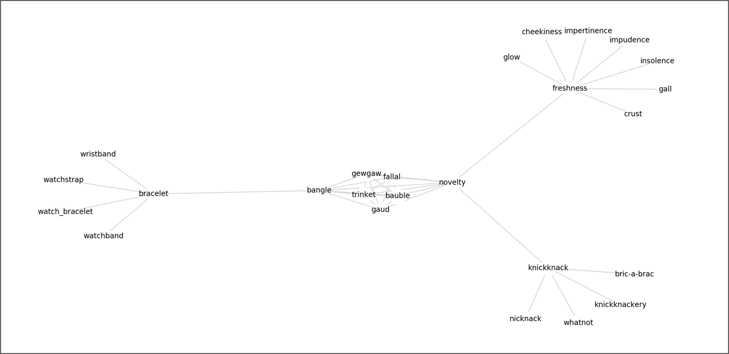
Figure 9-2. A spring layout helps to make visualization more manageable
In the next section, we will explore graph extraction and analysis techniques as they apply specifically to text.
Extracting Graphs from Text
One major challenge presents itself when the core dataset is text: where does the graph come from? The answer will usually depend on your problem domain, and generally speaking, the search for structural elements in semistructured or unstructured data will be guided by context-specific analytical questions.
To break this problem down into smaller substeps, we propose a simple graph analytics workflow for text as shown in Figure 9-3.
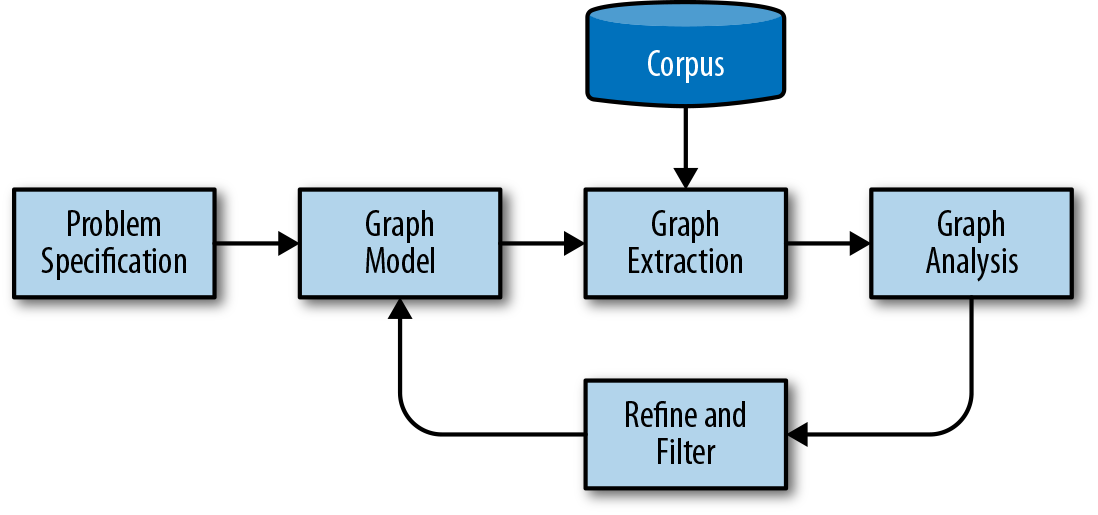
Figure 9-3. Workflow of graph analysis on text
In this workflow, we first use a problem statement to determine entities and their relationships. Using this schema, we can create a graph extraction methodology that uses the corpus, metadata, documents in the corpus, and phrases or tokens in the corpus’ documents to extract and link our data. The extraction method is a batch process that can run on the corpus and generate a graph that can be written to disk or stored in memory for analytical processing.
The graph analysis phase conducts computations on the extracted graph such as clustering, structural analysis, filtering, or querying and returns a new graph that is used as output for applications. Inspecting the results of the analytical process allows us to iterate on our method and schema, extracting or collapsing groups of nodes or edges as needed to ensure accurate, usable results.
Creating a Social Graph
Consider our corpus of news articles and our task of modeling relationships between different entities contained in the text. If our questions concern variations in coverage by different news outlets, we might build graph elements related to publication titles, author names, and syndication sources. However, if our goal is to aggregate multiple mentions of a single entity across many articles, our networks might encode forms of address like honorifics, in addition to demographic details. As such, entities of interest may reside in the structure of the documents themselves, or they may simply be contained in the text itself.
Let’s assume that our goal is merely to understand which people, places, and things are related to each other in our documents. In other words, we want to build a social network, which we can do with a series of transformations, as shown in Figure 9-4. We will begin constructing our graph using the EntityExtractor class we built in Chapter 7. Then we’ll add a custom transformer that finds pairs of related entities, followed by another custom transformer that transforms the paired entities into a graph.
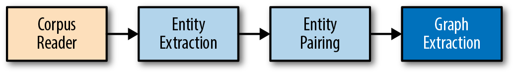
Figure 9-4. Entity graph extraction pipeline
Finding entity pairs
Our next step is to create an EntityPairs class that will expect documents that are represented as lists of entities (which is the result of a transform using the EntityExtractor class defined in Chapter 7). We want our class to function as a transformer inside a Scikit-Learn Pipeline, so it must inherit from BaseEstimator and TransformerMixin, as described in Chapter 4. We expect entities inside a single document to be related to each other, so we will add a pairs method, which uses the itertools.permutations function to identify every pair of entities that co-occur in the same document. Our transform method will call the pairs method on each document in the transformed corpus:
importitertoolsfromsklearn.baseimportBaseEstimator,TransformerMixinclassEntityPairs(BaseEstimator,TransformerMixin):def__init__(self):super(EntityPairs,self).__init__()defpairs(self,document):returnlist(itertools.permutations(set(document),2))deffit(self,documents,labels=None):returnselfdeftransform(self,documents):return[self.pairs(document)fordocumentindocuments]
Now we can systematically extract entities from documents and identify pairs. However, we don’t have a convenient way to differentiate pairs of entities that co-occur very frequently from those that appear together only once. We need a way of encoding the strength of the relationships between entities, which we’ll explore in the next section.
Property graphs
The mathematical model of a graph considers only sets of nodes and edges and can be represented as an adjacency matrix, which is useful for a large range of computations. However, it does not provide us with a mechanism for modeling the strength or type of any given relationship. Do the two actors appear in only one document together, or in many? Do they co-occur more frequently in certain genres of articles? In order to support this type of reasoning, we require some way of storing meaningful properties on our nodes and edges.
The property graph model allows us to embed more information into the graph, thereby extending computational ability. In a property graph, nodes are objects with incoming and outgoing edges and usually contain a type field, similar to a table in a relational database. Edges are objects with a source and target, and they typically contain a label field that identifies the type of relationship and a weight field that identifies the strength of the relationship. For graph-based text analytics, we generally use nodes to represent nouns and edges for verbs. Then later, when we move into a modeling phase, this allows us to describe the types of nodes, the labels of links, and the expected structure of the graph.
Implementing the graph extraction
We can now define a class, GraphExtractor, that will not only transform the entities into nodes, but also assign weights to their edges based on the frequency with which those entities co-occur in our corpus. Our class will initialize a NetworkX graph, and then our transform method will iterate through each document (which is a list of entity pairs), checking to see if there is already an edge between them in the graph. If there is, we will increment the edge’s weight property by 1. If the edge does not already exist in the graph, we use the add_edge method to create one with a weight of 1. As with our thesaurus graph construction, the add_edge method will also add a new node to the graph if it encounters a member of a pair that does not already exist in the graph:
importnetworkxasnxclassGraphExtractor(BaseEstimator,TransformerMixin):def__init__(self):self.G=nx.Graph()deffit(self,documents,labels=None):returnselfdeftransform(self,documents):fordocumentindocuments:forfirst,secondindocument:if(first,second)inself.G.edges():self.G.edges[(first,second)]['weight']+=1else:self.G.add_edge(first,second,weight=1)returnself.G
We can now streamline our entity extraction, entity pairing, and graph extraction steps in a Scikit-Learn Pipeline as follows:
if__name__=='__main__':fromreaderimportPickledCorpusReaderfromsklearn.pipelineimportPipelinecorpus=PickledCorpusReader('../corpus')docs=corpus.docs()graph=Pipeline([('entities',EntityExtractor()),('pairs',EntityPairs()),('graph',GraphExtractor())])G=graph.fit_transform(docs)(nx.info(G))
On a sample of the Baleen corpus, the graph that is constructed has the following statistics:
Name: Entity Graph
Type: Graph
Number of nodes: 29176
Number of edges: 1232644
Average degree:  84.4971
Insights from the Social Graph
We now have a graph model of the relationships between different entities from our corpus, so we can begin asking interesting questions about these relationships. For instance, is our graph a social network? In a social network, we would expect to see some very specific structures in the graph, such as hubs, or certain nodes that have many more edges than average.
In this section, we’ll see how we can leverage graph theory metrics like centrality measures, degree distributions, and clustering coefficients to support our analyses.
Centrality
In a network context, the most important nodes are central to the graph because they are connected directly or indirectly to the most nodes. Because centrality gives us a means of understanding a particular node’s relationship to its immediate neighbors and extended network, it can help us identify entities with more prestige and influence. In this section we will compare several ways of computing centrality, including degree centrality, betweenness centrality, closeness centrality, eigenvector centrality, and pagerank.
First, we’ll write a function that accepts an arbitrary centrality measure as a keyword argument and uses this measure to rank the top n nodes and assign each node a property with a score. NetworkX implements centrality algorithms as top-level functions that take a graph, G, as its first input and return dictionaries of scores for each node in the graph. This function uses the nx.set_node_attributes() function to map the scores computed by the metric to the nodes:
importheapqfromoperatorimportitemgetterdefnbest_centrality(G,metrics,n=10):# Compute the centrality scores for each vertexnbest={}forname,metricinmetrics.items():scores=metric(G)# Set the score as a property on each nodenx.set_node_attributes(G,name=name,values=scores)# Find the top n scores and print them along with their indextopn=heapq.nlargest(n,scores.items(),key=itemgetter(1))nbest[name]=topnreturnnbest
We can use this interface to assign scores automatically to each node in order to save them to disk or employ them as visual weights.
The simplest centrality metric, degree centrality, measures popularity by computing the neighborhood size (degree) of each node and then normalizing by the total number of nodes in the graph. Degree centrality is a measure of how connected a node is, which can be a signifier of influence or significance. If degree centrality measures how connected a given node is, betweenness centrality indicates how connected the graph is as a result of that node. Betweenness centrality is computed as the ratio of shortest paths that include a particular node to the total number of shortest paths.
Here we can use our entity extraction pipeline and nbest_centrality function to compare the top 10 most central nodes, with respect to degree and betweenness centrality:
fromtabulateimporttabulatecorpus=PickledCorpusReader('../corpus')docs=corpus.docs()graph=Pipeline([('entities',EntityExtractor()),('pairs',EntityPairs()),('graph',GraphExtractor())])G=graph.fit_transform(docs)centralities={"Degree Centrality":nx.degree_centrality,"Betweenness Centrality":nx.betweenness_centrality}centrality=nbest_centrality(G,centralities,10)formeasure,scoresincentrality.items():("Rankings for {}:".format(measure))((tabulate(scores,headers=["Top Terms","Score"])))("")
In our results, we see that degree and betweenness centrality overlap significantly in their ranks of the most central entities (e.g., “american,” “new york,” “trump,” “twitter”). These are the influential, densely connected nodes whose entities appear in more documents and also sit at major “crossroads” in the graph:
Rankings for Degree Centrality:
Top Terms      Score
----------    ---------
american       0.054093
new york       0.0500643
washington     0.16096
america        0.156744
united states  0.153076
los angeles    0.139537
republican     0.130077
california     0.120617
trump          0.116778
twitter        0.114447

Rankings for Betweenness Centrality:
Top Terms      Score
----------    ---------
american       0.224302
new york       0.214499
america        0.0258287
united states  0.0245601
washington     0.0244075
los angeles    0.0228752
twitter        0.0191998
follow         0.0181923
california     0.0181462
new            0.0180939
While degree and betweenness centrality might be used as a measure of overall celebrity, we frequently find that the most connected node has a large neighborhood, but is disconnected from the majority of nodes in the graph.
Let’s consider the context of a particular egograph, or subgraph, of our full graph that reframes the network from the perspective of one particular node. We can extract this egograph using the NetworkX method nx.ego_graph:
H=nx.ego_graph(G,"hollywood")
Now we have a graph that distills all the relationships to one specific entity (“Hollywood”). Not only does this dramatically reduce the size of our graph (meaning that subsequent searches will be much more efficient), this transformation will also enable us to reason about our entity.
Let’s say we want to identify entities that are closer on average to other entities in the Hollywood graph. Closeness centrality (implemented as nx.closeness_centrality in NetworkX) uses a statistical measure of the outgoing paths for each node and computes the average path distance to all other nodes from a single node, normalized by the size of the graph. The classic interpretation of closeness centrality is that it describes how fast information originating at a specific node will spread throughout the network.
By contrast, eigenvector centrality says that the more important nodes you are connected to, the more important you are, expressing “fame by association.” This means that nodes with a small number of very influential neighbors may outrank nodes with high degrees. Eigenvector centrality is the basis of several variants, including Katz centrality and the famous PageRank algorithm.
We can use our nbest_centrality function to see how each of these centrality measures produces differing determinations of the most important entities in our Hollywood egograph:
hollywood_centralities={"closeness":nx.closeness_centrality,"eigenvector":nx.eigenvector_centrality_numpy,"katz":nx.katz_centrality_numpy,"pagerank":nx.pagerank_numpy,}hollywood_centrality=nbest_centrality(H,hollywood_centralities,10)formeasure,scoresinhollywood_centrality.items():("Rankings for {}:".format(measure))((tabulate(scores,headers=["Top Terms","Score"])))("")
Our results show that the entities with the highest closeness centrality (e.g., “video,” “british,” “brooklyn”), are not particularly ostentatious, perhaps instead serving as the hidden forces connecting more prominent celebrity structures. Eigenvector, PageRank, and Katz centrality all reduce the impact of degree (e.g., the most commonly occurring entities) and have the effect of showing “the power behind the scenes,” highlights well-connected entities (“republican,” “obama”) and sidekicks:
Rankings for Closeness Centrality:
Top Terms      Score
----------    ---------
hollywood       1
new york        0.687801
los angeles     0.651051
british         0.6356
america         0.629222
american        0.625243
video           0.621315
london          0.612872
china           0.612434
brooklyn        0.607227

Rankings for Eigenvector Centrality:
Top Terms       Score
----------     ---------
hollywood       0.0510389
new york        0.0493439
los angeles     0.0485406
british         0.0480387
video           0.0480122
china           0.0478956
london          0.0477556
twitter         0.0477143
new york city   0.0476534
new             0.0475649

Rankings for PageRank Centrality:
Top Terms       Score
----------     ---------
hollywood       0.0070501
american        0.00581407
new york        0.00561847
trump           0.00521602
republican      0.00513387
america         0.00476237
donald trump    0.00453808
washington      0.00417929
united states   0.00398346
obama           0.00380977

Rankings for Katz Centrality:
Top Terms           Score
----------         ---------
video               0.107601
washington          0.104191
chinese             0.1035
hillary             0.0893112
cleveland           0.087653
state               0.0876141
muslims             0.0840494
editor              0.0818608
paramount pictures  0.0801545
republican party    0.0787887
Tip
For both betweenness and closeness centrality, all shortest paths in the graph must be computed, meaning they can take a long time to run and may not scale well to larger graphs. The primary mechanism of improving performance is to use a lower-level implementation that may also parallelize the computation. Graph-tool has mechanisms for both betweenness and closeness centrality, and is a good option for computing against larger graphs.
Structural analysis
As we saw earlier in this chapter, visual analysis of graphs enables us to detect interesting patterns in their structure. We can plot our Hollywood egograph to explore this structure as we did earlier with our thesaurus graph, using the nx.spring_layout method, passing in a k value to specify the minimum distance between nodes, and an iterations keyword argument to ensure the nodes are separate enough to be legible (Figure 9-5).
H=nx.ego_graph(G,"hollywood")edges,weights=zip(*nx.get_edge_attributes(H,"weight").items())pos=nx.spring_layout(H,k=0.3,iterations=40)nx.draw(H,pos,node_color="skyblue",node_size=20,edgelist=edges,edge_color=weights,width=0.25,edge_cmap=plt.cm.Pastel2,with_labels=True,font_size=6,alpha=0.8)plt.show()
Many larger graphs will suffer from the “hairball effect,” meaning that the nodes and edges are so dense as to make it difficult to effectively discern meaningful structures. In these cases, we often instead try to inspect the degree distribution for all nodes in a network to inform ourselves about its overall structure.
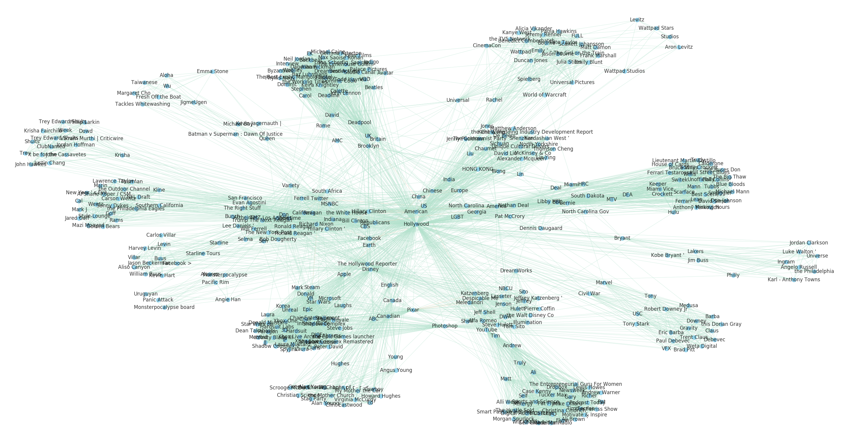
Figure 9-5. Relationships to Hollywood in the Baleen corpus
We can examine this distribution using Seaborn’s distplot method, setting the norm_hist parameter to True so that the height will display degree density rather than raw count:
importseabornassnssns.distplot([G.degree(v)forvinG.nodes()],norm_hist=True)plt.show()
In most graphs, the majority of nodes have relatively low degree, so we generally expect to observe a high amount of right-skew in their degree distributions, such as in the Baleen Entity Graph plot shown in the upper left of Figure 9-6. The small number of nodes with the highest degrees are hubs due to their frequent occurrence and large number of connections across the corpus.
Note
Certain social networks, called scale-free networks, exhibit power law distributions, and are associated with particularly high fault-tolerance. Such structures indicate a resilient network that doesn’t rely on any single node (in our case, perhaps a person or organization) to keep the others connected.
Interestingly, the degree distributions for certain ego graphs display remarkably different behavior, such as with the Hollywood ego graph exhibiting a nearly symmetric probability distribution, as shown in the upper right of Figure 9-6.
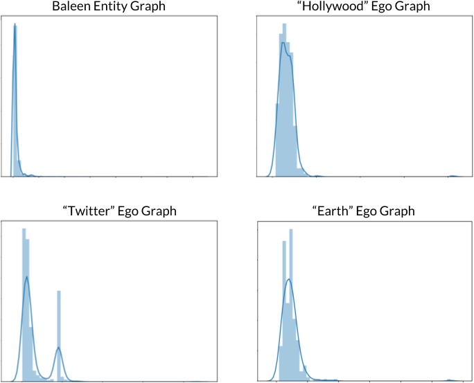
Figure 9-6. Histograms of degree distributions
Other useful structural measures of a network are its clustering coefficient (nx.average_clustering) and transitivity (nx.transitivity), both of which can be used to assess how social a network is. The clustering coefficient is a real number that is 0 when there is no clustering and 1 when the graph consists entirely of disjointed cliques (nx.graph_number_of_cliques). Transitivity tells us the likelihood that two nodes with a common connection are neighbors:
("Baleen Entity Graph")("Average clustering coefficient: {}".format(nx.average_clustering(G)))("Transitivity: {}".format(nx.transitivity(G)))("Number of cliques: {}".format(nx.graph_number_of_cliques(G)))("Hollywood Ego Graph")("Average clustering coefficient: {}".format(nx.average_clustering(H)))("Transitivity: {}".format(nx.transitivity(H)))("Number of cliques: {}".format(nx.graph_number_of_cliques(H)))
Baleen Entity Graph
Average clustering coefficient: 0.7771459590548481
Transitivity: 0.29504798606584176
Number of cliques: 51376

Hollywood Ego Graph
Average clustering coefficient: 0.9214236425410913
Transitivity: 0.6502420989124886
Number of cliques: 348
In the context of our entity graph, the high clustering and transitivity coefficients suggest that our network is extremely social. For instance, in our “Hollywood” ego graph, the transitivity suggests that there is a 65 percent chance that any two entities who share a common connection are themselves neighbors!
Note
The small world phenomenon can be observed in a graph where, while most nodes are not direct neighbors, nearly all can be reached from every other node within a few hops. Small world networks can be identified from structural features, namely that they often contain many cliques, have a high clustering coefficient, and have a high degree of transitivity. In the context of our entity graph, this would suggest that even in a network of strangers, most are nevertheless linked through a very short chain of acquaintances.
Entity Resolution
One challenge we have yet to discuss is the multiplicity of ways in which our entities can appear. Because we have performed little or no normalization on our extracted entities, we can expect to see many variations in spelling, forms of address, and naming conventions, such as nicknames and acronyms. This will result in multiple nodes that reference a single entity (e.g., “America,” “US,” and “the United States” all appear as nodes in the graph).
In Figure 9-7, we see multiple, often ambiguous references to “Hilton,” which refers not only to the family as a whole, but also to individual members of the family, to the corporation, and to specific hotel facilities in different cities. Ideally we would like to identify nodes that correspond to multiple references so that we can resolve them into unique entity nodes.
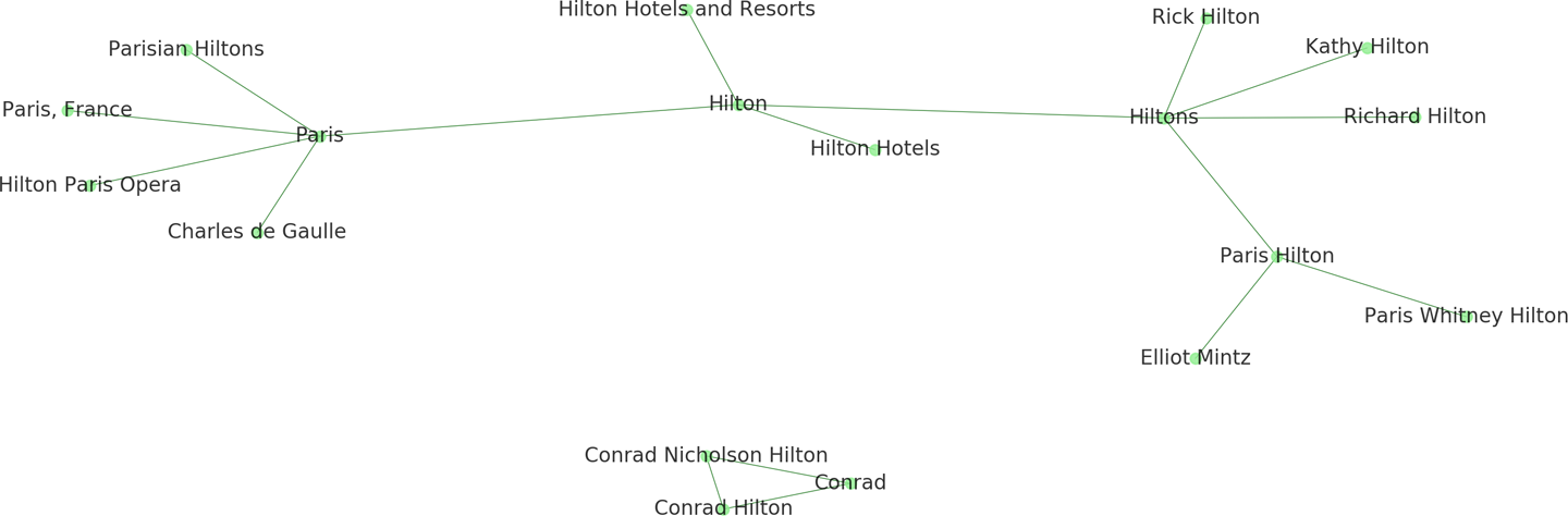
Figure 9-7. Multiple entity references within a graph
Entity resolution refers to computational techniques that identify, group, or link digital mentions (records) of some object in the real world (an entity). Part of the data wrangling process is performing entity resolution to ensure that all mentions to a single, unique entity are collected together into a single reference.
Tasks like deduplication (removing duplicate entries), record linkage (joining two records together), and canonicalization (creating a single, representative record for an entity) rely on computing the similarity of (or distance between) two records and determining whether they are a match.
Entity Resolution on a Graph
As Bhattacharya and Getoor (2005)2 explain, a graph with multiple nodes corresponding to single entities is not actually an entity graph, but a reference graph. Reference graphs are very problematic for semantic reasoning tasks, as they can distort and misrepresent the relationships between entities.
Entity resolution will get us closer to analyzing and extracting useful information about the true structure of a real-world network, reducing the obscurity caused by the many ways language allows us to refer to the same entity. In this section we’ll explore a methodology where we include entity resolution as an added step in our graph extraction pipeline, as shown in Figure 9-8.

Figure 9-8. Entity graph extraction pipeline
To begin resolving the entities in our Hilton graph, we will first define a function pairwise_comparisons that takes as input a NetworkX graph and uses the itertools.combinations method to create a generator with every possible pair of nodes:
importnetworkxasnxfromitertoolsimportcombinationsdefpairwise_comparisons(G):"""Produces a generator of pairs of nodes."""returncombinations(G.nodes(),2)
Unfortunately, even a very small dataset such as our Hilton graph of 18 nodes will generate 153 pairwise comparisons. Given that similarity comparison is usually an expensive operation involving dynamic programming and other resource-intensive computing techniques, this clearly will not scale well. There are a few simple things we can do, such as eliminating pairs that will never match, to reduce the number of pairwise comparisons. In order to make decisions like these, either in an automatic fashion or by proposing pairs of records to a user, we first need some mechanism to expose likely similar matches and weed out the obvious nonduplicates. One method we can use is blocking.
Blocking with Structure
Blocking is the strategic reduction of the number of pairwise comparisons that are required using the structure of a natural graph. Blocking provides entity resolution with two primary benefits: increasing the performance by reducing the number of computations and reducing the search space to propose possible duplicates to a user.
One reasonable assumption we might make is that if two nodes both have an edge to the same entity (e.g., “Hilton Hotels” and “Hilton Hotels and Resorts” both have edges to “Hilton”), they are more likely to be references to the same entity. If we can inspect only the most likely matches, that could dramatically reduce the number of comparisons we have to make. We can use the NetworkX neighbors method to compare the edges of any two given nodes and highlight only the pairwise comparisons that have very similar neighborhoods:
defedge_blocked_comparisons(G):"""A generator of pairwise comparisons, that highlights comparisonsbetween nodes that have an edge to the same entity."""forn1,n2inpairwise_comparisons(G):hood1=frozenset(G.neighbors(n1))hood2=frozenset(G.neighbors(n2))ifhood1&hood2:yieldn1,n2
Fuzzy Blocking
Even with blocking, there are still some unnecessary comparisons. For example, even though “Kathy Hilton” and “Richard Hilton” both have an edge to “Hiltons,” they do not refer to the same person. We want to be able to further uncomplicate the graph by identifying the most likely approximate matches using some kind of similarity measure that can compute the distance between “Kathy Hilton” and “Richard Hilton.”
There are a number of methods for computing string distance, many of which depend on the use case. Here we will demonstrate an implementation that leverages the partial_ratio method from the Python library fuzzywuzzy, which uses Levenshtein distance to compute the number of deletions, insertions, and substitutions required to transform the first string into the second.
We will define a similarity function that takes as input two NetworkX nodes. Our function will score the distance between the string name labels for each node, the distance between their Spacy entity types (stored as a node attributes), and return their mean:
fromfuzzywuzzyimportfuzzdefsimilarity(n1,n2):"""Returns the mean of the partial_ratio score for each field in the twoentities. Note that if they don't have fields that match, the score willbe zero."""scores=[fuzz.partial_ratio(n1,n2),fuzz.partial_ratio(G.node[n1]['type'],G.node[n2]['type'])]returnfloat(sum(sforsinscores))/float(len(scores))
If two entities have almost the same name (e.g., “Richard Hilton” and “Rick Hilton”), and are also both of the same type (e.g., PERSON), they will get a higher score than if they have the same name but are of different types (e.g., one PERSON and one ORG).
Now that we have a way to identify high-probability matches, we can incorporate it as a filter into a new function, fuzzy_blocked_comparison. This function will iterate through each possible pair of nodes and determine the amount of structural overlap between them. If there is significant overlap, it will compute their similarity and yield pairs with similar neighborhoods who are sufficiently similar (above some threshold, which we implement as a keyword argument that defaults to a 65 percent match):
deffuzzy_blocked_comparisons(G,threshold=65):"""A generator of pairwise comparisons, that highlights comparisons betweennodes that have an edge to the same entity, but filters out comparisonsif the similarity of n1 and n2 is below the threshold."""forn1,n2inpairwise_comparisons(G):hood1=frozenset(G.neighbors(n1))hood2=frozenset(G.neighbors(n2))ifhood1&hood2:ifsimilarity(n1,n2)>threshold:yieldn1,n2
This is a very efficient way of reducing pairwise comparisons, because we use the computationally less intensive neighborhood comparison first, and only then proceed to the more expensive string similarity measure. The reduction in total comparisons is significant:
definfo(G):"""Wrapper for nx.info with some other helpers."""pairwise=len(list(pairwise_comparisons(G)))edge_blocked=len(list(edge_blocked_comparisons(G)))fuzz_blocked=len(list(fuzzy_blocked_comparisons(G)))output=[""]output.append("Number of Pairwise Comparisons: {}".format(pairwise))output.append("Number of Edge Blocked Comparisons: {}".format(edge_blocked))output.append("Number of Fuzzy Blocked Comparisons: {}".format(fuzz_blocked))returnnx.info(G)+"\n".join(output)
Name: Hilton Family
Type: Graph
Number of nodes: 18
Number of edges: 17
Average degree:   1.8889
Number of Pairwise Comparisons: 153
Number of Edge Blocked Comparisons: 32
Number of Fuzzy Blocked Comparisons: 20
We have now identified the 20 pairs of nodes with the highest likelihood of being references to the same entity, a more than 85 percent reduction in the total possible pairwise comparisons.
Now we can imagine creating a custom transformer that we can chain together with the rest of our pipeline to transform our reference graph into a list of fuzzy edge blocked comparisons. For instance, a FuzzyBlocker might begin with these methods and add others depending on the specific requirements of the entity resolution problem:
fromsklearn.baseimportBaseEstimator,TransformerMixinclassFuzzyBlocker(BaseEstimator,TransformerMixin):def__init__(self,threshold=65):self.threshold=thresholddeffit(self,G,y=None):returnselfdeftransform(self,G):returnfuzzy_blocked_comparisons(G,self.threshold)
Depending on the context and the fuzzy match threshold we have specified, these blocked nodes could be collapsed into single nodes (updating the edge properties as necessary), or be passed to a domain expert for manual inspection. In either case, entity resolution will often be a critical first step in building quality data products, and as we’ve seen in this section, graphs can make this process both more efficient and effective.
Conclusion
Graphs are used to represent and model complex systems in the real world, such as communication networks and biological ecosystems. However, they can also be used more generally to structure problems in meaningful ways. With a little creativity, almost any problem can be structured as a graph.
While graph extraction may seem challenging initially, it is just another iterative process that requires clever language processing and creative modeling of the target data. Just as with the other model families we have explored in this book, iterative refinement and analysis is part of the model selection triple, and techniques like normalization, filtering, and aggregation can be added to improve performance.
However, in contrast to other model families we have explored in previous chapters, the graph model family contains algorithms whose computations are composed of traversals. From a local node, the computation can use information from neighboring nodes extracted by traveling along the edges that connect any two nodes. Such computations expose nodes that are connected, show how connections form, and identify which nodes are most central to the network. Graph traversals enable us to extract meaningful information from documents without requiring vast amounts of prior knowledge and ontologies.
Graphs can embed complex semantic representations in a compact form. As such, modeling data as networks of related entities is a powerful mechanism for analytics, both for visual analyses and machine learning. Part of this power comes from performance advantages of using a graph data structure, and the other part comes from an inherent human ability to intuitively interact with small networks.
The lesson of graph analytics is an important one; text analysis applications are made and broken by their interpretability—if the user doesn’t understand it, it doesn’t matter how insightful the result is. Next, in Chapter 10 we will continue to follow the thread of human–computer interaction we began in Chapter 8 and pursued in this chapter, considering instead how the application of chatbots to everyday language-based tasks can augment the user’s experience.
1 George A. Miller and Christiane Fellbaum, WordNet: A Lexical Database for English, (1995) http://bit.ly/2GQKXmI
2 Indrajit Bhattacharya and Lise Getoor, Entity Resolution in Graph Data, (2005) http://bit.ly/2GQKXDe